$4d$ higgsed network calculus and elliptic DIM algebra

Abstract

Supersymmetric gauge theories of certain class possess a large hidden nonperturbative symmetry described by the Ding-Iohara-Miki (DIM) algebra which can be used to compute their partition functions and correlators very efficiently. We lift the DIM-algebraic approach developed to study holomorphic blocks of $3d$ linear quiver gauge theories one dimension higher. We employ an algebraic construction in which the underlying trigonometric DIM algebra is elliptically deformed, and an alternative geometric approach motivated by topological string theory. We demonstrate the equivalence of these two methods, and motivated by this, prove that elliptic DIM algebra is isomorphic to the direct sum of a trigonometric DIM algebra and an additional Heisenberg algebra.

1 Introduction

String theory provides an effective framework for studying supersymmetric gauge theories in various dimensions using geometric and algebraic tools. These constructions are connected to each other by string dualities. Depending on the properties of the gauge theories we would like to study in detail one construction could shed more light compared to the others. Moreover, these constructions utilize geometric and algebraic approaches and intertwine them. The present paper aims to study further the connection between the elliptic Ding-Iohara-Miki (DIM) algebras [1, 2] and topological string theory motivated approaches.

We can construct supersymmetric gauge theories using webs of branes in type IIB string theory. These webs are trivalent graphs on a plane, and such graphs are shown to be identical to the toric diagrams that are used to engineer the gauge theory in type IIA/M-theory compactifications [3]. The (refined) topological vertex [4] is employed to calculate the topological string free energy for the toric Calabi-Yau threefold which is identical to the instanton free energy after the proper identification of the gauge theory parameters with the Kähler classes of the geometry. Although the topological vertex is constructed as a geometric device to count maps, the quantum algebraic structure behind it was discovered in [5]. In particular, two different versions of the refined topological vertex were shown to be matrix elements of the same intertwining operator of Fock representations of the DIM algebra.

The DIM algebra also plays the central role in the $q$-deformed version of the well-known Alday-Gaiotto-Tachikawa (AGT) relation. The connection between the DIM algebra and supersymmetric gauge theories have been exploited in various directions. The fiber-base duality in geometric engineering [6] or its type IIB interpretation as $S$-duality is mapped [7] to the Miki automorphism [2], [8]. DIM also provides a universal way to understand the $qq$-characters [9], [10] using quiver gauge theories in different dimensions [11], [12]. A network matrix model is introduced by composing DIM intertwiners according to the data encoded in toric diagrams, leading to $q$-deformed Dotsenko-Fateev integrals corresponding to $q$-deformed vertex operator algebras. Recently, the Higgsing construction has been employed to calculate the holomorphic blocks of $3d$ ${\mathcal{N}}=2^{*}$ theories [13]. Higgsing involves tuning certain mass and Coulomb branch parameters of a ‘‘parent’’ $5d$ theory to reach the point on the moduli space where the Higgs and the Coulomb branches meet. The $3d$ theory is nothing but the worldvolume theory of the vortices in the Higgs phase of the parent $5d$ theory [14, 15, 16].

Recently a new approach for direct computation of the $3d$ holomorphic blocks using the vector representation of the DIM algebra was proposed, the higgsed network calculus [17]. In this approach one engineers the $3d$ theories by suspending D3 branes between NS5 branes, as opposed to building the parent $5d$ theories from a web of 5-branes, without D3 branes. In the 5-brane web we associate a Fock space to each one of the 5-branes with central charges that match the $(p,q)$ charges of the corresponding brane. The web encodes the brane charges in terms of the slopes in the associated trivalent graph. However, when a D3 brane is connected to an NS5 brane, it does not bend the NS5 brane. Correspondingly a vector representation does not have central charges and can be identified with a D3 brane. The intertwining operator playing the role of the D3-NS5 brane junction, is $\Phi(w):\mathcal{F}^{(1,0),q,t^{-1}}_{u}\otimes\mathcal{V}^{q}_{w}\to\mathcal{F}_{tu}^{(1,0),q,t^{-1}}$, where $\mathcal{V}$ stands for the vector representation and $\mathcal{F}$ is for Fock representation.

In this work, we lift this construction one dimension higher by studying the elliptic deformation of the DIM algebra proposed in [18] as well as employing the compactification of the geometry in the direction of the 5-brane, following [19]. In fact, it was argued in [20, 21] that the compactification of the toric diagram and the elliptic deformation are equivalent extension of the AGT relation to a relation between $6d$ uplift of the superconformal gauge theory and the elliptic version of the Virasoro algebra. The elliptically deformed Dotsenko-Fateev (DF) integrals were shown to reproduce the $6d$ instanton generating functions that were computed using the refined topological vertex. In this work, we also study the relation between the compactification and elliptic DIM algebra.

According to [18], an elliptic deformation of any vertex operator given in free field representation can be obtained algorithmically. This is done by doubling the number of free bosons and then rescaling their modes by a factor containing the elliptic deformation parameter. The algorithm produces manifestly elliptic results for correlators of the deformed vertex operators. For example, before the elliptic deformation the two point functions between the $q$-$W$-algebra screening charges are expressed through the so-called $q$-Pochhammer functions. Once the screening charges are elliptically deformed following the aforementioned prescription, their two point functions turn out to be given in terms of the elliptic gamma functions, the natural generalizations of the $q$-Pochhammer functions. On the other hand, if we compactify along a single 5-brane with a number of intertwining (as well as dual intertwining) operators, we do not obtain a manifestly elliptic expression. However, once the flavor symmetries are gauged by gluing multiple compactified 5-branes, the DF integrands become elliptic functions, and match what we compute using the elliptic deformation of the vertex operators.

Having worked out the $4d$ lift of the higgsed network, we investigate further the structure of the elliptic DIM algebras. We propose an alternative but equivalent interpretation to the elliptic deformation [18] in terms of thermo field doubles. We construct an isomorphism between the elliptic DIM algebra and a direct sum of trigonometric DIM algebra and a Heisenberg algebra. Both the trigonometric and the elliptic DIM algebras are endowed with a Hopf algebra structure. We conjecture that the coproducts are related after a nontrivial Drinfeld twist.

The paper is organized as follows. In sec. 2, we start with a brief review of the elliptic deformation introduced in [18], and compute the lift of the vacuum expectation value for different configurations of intertwining operators which we will use as building blocks to obtain the partition functions of $4d$ theories by gluing them to each other. In sec. 3, we will compute matrix elements for the same type of insertions of intertwining operators to compute their traces. Section 4 is reserved to check that the elliptic deformation of the intertwining operators between a vector and a Fock space representations are indeed the intertwining operators of the elliptic DIM algebra. In sec. 5, we reinterpret the elliptic deformation of the DIM algebra from thermal quantum field theory perspective and show that the elliptic DIM algebra is just the product of two simpler algebras, the trigonometric DIM algebra and a Heisenberg algebra. We argue that the trace in the usual DIM algebra is just vacuum expectation value in the elliptic DIM. In the Appendices, we collect some definitions, conventions and technical details that we skip in the main text.

2 Elliptic Deformation of Vertex Operators

A one parameter elliptic deformation of the DIM algebra was first introduced in [22] based on quasi-Hopf twist with the aim to realize the elliptic version of the Macdonald operator of [23]. The elliptic kernel function associated with this difference operator is proposed in [24]. The precise connection between the elliptic deformation of [22] and the elliptic kernel function remains still unclear.

Another elliptic deformation of the DIM algebra was presented in [18] to establish the aforementioned missing connection to the elliptic kernel function. This deformation does not only depend on an extra parameter related to the ellipticity but also requires doubling of the Heisenberg algebra used in free field representation of the algebra. In [20, 21], this elliptic form of DIM algebra was shown to be the relevant deformation in lifting the AGT conjecture to $6d$ theory on the gauge theory side, and elliptic conformal blocks on the CFT side. Moreover, at the special points on the moduli space of the $6d$ theory the instanton partition function coincides with the vortex partition function supported on co-dimension two subspaces of spacetime [21]. The reduction of the instanton partition function to the vortex partition functions was previously observed for $5d$ bulk theory in [16], and ealier for $4d$ theories in [14]. Recently, a direct approach to obtain the vortex partition function using the intertwining operators of vector representations of the DIM algebra has been proposed. Motivated by the results of [20, 21], we propose an elliptic deformation of the vector intertwiner (higgsed vertex) according to the elliptic recipe of [18].

An algorithmic approach to elliptic deformation of a vertex operator with a free field realization was introduced in [18], and we briefly review it here for completeness. Suppose that we have a vertex operator of the form

$$X(z)=\exp\left(\sum_{n\geq 1}X_{-n}^{-}a_{-n}z^{n}\right)\exp\left(\sum_{n\geq 1}X_{n}^{+}a_{n}z^{-n}\right),$$ (1)

where $X^{\pm}_{\pm n}$ are generically complex numbers, and the operators $\{a_{n}\}_{n\in\mathbb{Z}\backslash\{0\}}$ satisfy the $q$-deformed version of the Heisenberg algebra,

$$[a_{m},a_{n}]=m\frac{1-q^{|m|}}{1-t^{|m|}}\delta_{m+n,0}.$$ (2)

The elliptic deformation involves two steps: in the first one, we deform the Heisenberg algebra (2) with an additional factor depending on the elliptic parameter $p$ and introduce an additional deformed Heisenberg algebra:

$$[a_{m},a_{n}]=m(1-p^{|m|})\frac{1-q^{|m|}}{1-t^{|m|}}\delta_{m+n,0},\qquad[b_{m},b_{n}]=m\frac{1-p^{|m|}}{(qt^{-1}p)^{|m|}}\frac{1-q^{|m|}}{1-t^{|m|}}\delta_{m+n,0}.$$ (3)

The new Heisenberg algebra commutes with the existing one, $[a_{m},b_{n}]=0$.

The second setup consists of writing down two auxiliary vertex operator in terms of the deformed modes $\{a_{n}\}$ and $\{b_{n}\}$,

$$X_{b}(p;z) \stackrel{{\scriptstyle\mathrm{def}}}{{=}}\exp\left(-\sum_{n\geq 1}\frac{p^{n}}{1-p^{n}}X^{-}_{n}b_{-n}z^{-n}\right)\exp\left(-\sum_{n\geq 1}\frac{p^{n}}{1-p^{n}}X^{+}_{-n}b_{n}z^{n}\right),$$ (4)

$$X_{a}(p;z) \stackrel{{\scriptstyle\mathrm{def}}}{{=}}\exp\left(\sum_{n\geq 1}\frac{1}{1-p^{n}}X^{-}_{-n}a_{-n}z^{n}\right)\exp\left(\sum_{n\geq 1}\frac{1}{1-p^{n}}X^{+}_{n}a_{n}z^{-n}\right).$$ (5)

The elliptic deformation $X(p;z)$ of the operator $X(z)$ is defined as a product of the auxiliary operators (4) and (5):

$$X^{(e)}(z)\stackrel{{\scriptstyle\mathrm{def}}}{{=}}X_{a}(p;z)X_{b}(p;z).$$ (6)

The (trigonometric) intertwining operator $\Phi(w)$ associated with D3-NS5 junction [17] is given by

$$\Phi(w)=e^{-\epsilon_{2}Q}w^{\frac{P}{\epsilon_{1}}}\exp\left(-\sum_{n\geq 1}\frac{w^{n}}{n}\frac{1-t^{-n}}{1-q^{n}}a_{-n}\right)\exp\left(\sum_{n\geq 1}\frac{w^{-n}}{n}\frac{1-t^{n}}{1-q^{-n}}a_{n}\right).$$ (7)

where $\epsilon_{1}=\ln q$, $\epsilon_{2}=-\ln t$ and $P$ and $Q$ are the momentum and momentum shift operators respectively. We will use a graphical representation of the intertwining operators to make the structure of intertwiner networks more transparent. We also emphasize that the line in the diagram can be viewed as branes: vector representations (dashed lines) are D3 branes and Fock representations (solid lines) are 5-branes. We thus draw:

$$\Phi(w)=\quad\includegraphics[valign={c}]{figures/vect-vert-crop}$$ (8)

Note that the intertwining operator (7) is precisely in the form required by the elliptic deformation algorithm reviewed above. We thus apply the elliptic deformation to it as prescribed and thus obtain the intertwiner $\Phi^{(e)}(w)$. It is straightforward to work out the elliptic versions of a network with a pair of intertwining operators:

(9)

We get

$$\langle t^{2}u,\varnothing|\Phi^{(e)}(w_{1})\Phi^{(e)}(w_{2})|u,\varnothing\rangle=w_{1}^{\log_{q}u+\beta}w_{2}^{\log_{q}u}\frac{\Gamma_{p,q}(qw_{2}/w_{1})}{\Gamma_{p,q}(qw_{2}/tw_{1})},$$ (10)

where $\Gamma_{p,q}(z)$ is the elliptic gamma function. The superscript $(e)$ indicates the elliptic version of the intertwining operator. Note that in the limit when we turn off the elliptic deformation by taking the limit $p\rightarrow 0$, and using the fact that the elliptic gamma function becomes inverse $q$-Pochhammer symbol in this limit

$$\Gamma_{p,q}(z)\rightarrow\frac{1}{(z;q)_{\infty}},\,\,\mbox{as}\,\,p\rightarrow 0,$$ (11)

we can recover the original result of [17]. Furthermore, we can put this expression in a nicer form using the reflection property of the elliptic gamma function and a nice relation with the $\theta$-function:

$$\langle t^{2}u,\varnothing|\Phi^{(e)}(w_{1})\Phi^{(e)}(w_{2})|u,\varnothing\rangle=w_{1}^{\log_{q}u+\beta}w_{2}^{\log_{q}u}\,\frac{\theta_{q}(tw_{1}/w_{2})}{\theta_{q}(w_{1}/w_{2})}\frac{\Gamma_{p,q}(tw_{1}/w_{2})}{\Gamma_{p,q}(w_{1}/w_{2})}.$$ (12)

We can extend this result to $n$ insertions of intertwining operators at points $w_{1}$, …, $w_{n}$,

$$\includegraphics[valign={c}]{figures/strip-2-crop}=A(\vec{w})\left(\prod_{i=1}^{n}w_{i}^{\log_{q}u+\beta(i-1)}\right)\prod_{i<j}\frac{\Gamma_{p,q}(tw_{i}/w_{j})}{\Gamma_{p,q}(w_{i}/w_{j})}$$ (13)

where $A(\vec{w})$ remains invariant under the elliptic deformation,

$$A(\vec{w})=\prod_{i<j}\left[\left(\frac{w_{i}}{w_{j}}\right)^{\beta}\frac{\theta_{q}\left(t\frac{w_{i}}{w_{j}}\right)}{\theta_{q}\left(\frac{w_{i}}{w_{j}}\right)}\right].$$ (14)

The dual intertwining operator $\Phi^{*}(y)$ also has an explicit free field representation

$$\includegraphics[valign={c}]{figures/vect-vert-dual-crop}\quad=\Phi^{*}(y)=\\ =e^{\epsilon_{2}Q}y^{\beta-\frac{P}{\epsilon_{1}}}\exp\left[\sum_{n\geq 1}\frac{y^{n}}{n}\left(\frac{t}{q}\right)^{\frac{n}{2}}\frac{1-t^{-n}}{1-q^{n}}a_{-n}\right]\exp\left[-\sum_{n\geq 1}\frac{y^{-n}}{n}\left(\frac{t}{q}\right)^{\frac{n}{2}}\frac{1-t^{n}}{1-q^{-n}}a_{n}\right],$$ (15)

and can be elliptically deformed by the above prescription. We denote the resulting operator $\Phi^{(e)*}(y)$.

It is straightforward to compute the matrix element of the elliptic deformation of $n$ dual intertwining operators in a similar fashion,

$$\includegraphics[valign={c}]{figures/strip-3-crop}\quad=\left(\prod_{i=1}^{n}y_{i}^{-\log_{q}u+\beta(i-n+1)}\right)\prod_{i<j}\frac{\Gamma_{p,q}(ty_{j}/y_{i})}{\Gamma_{p,q}(y_{j}/y_{i})}.$$ (16)

A combination of $n$ intertwining and $m$ dual intertwining operators is another possible configuration that we will encounter in what follows. We can order the intertwiners in two separate groups:

$$\includegraphics[valign={c}]{figures/strip-4-crop}\quad=A(\vec{w})B(\vec{w},\vec{y})\left(\prod_{i=1}^{n}w_{i}^{\log_{q}u+\beta(i-2m-1)}\right)\times\\ \times\left(\prod_{i=1}^{m}y_{i}^{-\log_{q}u+\beta(i-2n+1)}\right)\prod_{k<l}^{n}\frac{\Gamma_{p,q}\left(t\frac{w_{k}}{w_{l}}\right)}{\Gamma_{p,q}\left(\frac{w_{k}}{w_{l}}\right)}\prod_{i<j}^{m}\frac{\Gamma_{p,q}\left(t\frac{y_{j}}{y_{i}}\right)}{\Gamma_{p,q}\left(t\frac{y_{j}}{y_{i}}\right)}\prod_{a=1}^{m}\prod_{b=1}^{n}\frac{\Gamma_{p,q}\left(\sqrt{\frac{q}{t}}\frac{w_{b}}{y_{a}}\right)}{\Gamma_{p,q}\left(t\sqrt{\frac{q}{t}}\frac{w_{b}}{y_{a}}\right)},$$ (17)

where an additional $q$-periodic prefactor reads

$$B(\vec{w},\vec{y})=\prod_{a=1}^{m}\prod_{b=1}^{n}\left[\left(\frac{y_{a}}{w_{b}}\right)^{\beta}\frac{\theta_{q}\left(t\sqrt{\frac{q}{t}}\frac{y_{a}}{w_{b}}\right)}{\theta_{q}\left(\sqrt{\frac{q}{t}}\frac{y_{a}}{w_{b}}\right)}\right].$$ (18)

Note that $A(\vec{w})$ and $B(\vec{w},\vec{y})$ remain invariant after the elliptic deformation.

We also compute the commutators of the intertwining operators, which will allow us to reorder the products like that in (17):

1. Commutation of $\Phi^{(e)}(w_{1})$ with $\Phi^{(e)}(w_{2})$:

   $$\includegraphics[valign={c}]{figures/r-up-1-crop}\quad=\left[\left(\frac{w_{1}}{w_{2}}\right)^{\beta}\frac{\theta_{q}\left(t\frac{w_{1}}{w_{2}}\right)}{\theta_{q}\left(\frac{w_{1}}{w_{2}}\right)}\right]R^{(e)}\left(\frac{w_{1}}{w_{2}}\right)\times\quad\includegraphics[valign={c}]{figures/r-up-2-crop}$$ (19)

   where we define the elliptic $R$-matrix for vector representations

   $$R^{(e)}\left(x\right)=\frac{\Gamma_{p,q}\left(\frac{q}{t}x\right)\Gamma_{p,q}\left(tx\right)}{\Gamma_{p,q}\left(qx\right)\Gamma_{p,q}\left(x\right)}.$$ (20)

   Once again, the $q$-periodic prefactor remains invariant under the elliptic deformation. The elliptic $R$-matrix $R^{(e)}$ tends to the original trigonometric $R$-matrix [17] in the limit $p\rightarrow 0$.

2. Commutation of $\Phi^{*(e)}(y_{1})$ with $\Phi^{*(e)}(y_{2})$:

   $$\includegraphics[valign={c}]{figures/r-down-1-crop}\quad=\left[\left(\frac{y_{1}}{y_{2}}\right)^{\beta}\frac{\theta_{q}\left(\frac{y_{2}}{y_{1}}\right)}{\theta_{q}\left(t\frac{y_{2}}{y_{1}}\right)}\right]\frac{1}{R^{(e)}\left(\frac{y_{1}}{y_{2}}\right)}\times\quad\includegraphics[valign={c}]{figures/r-down-2-crop}$$ (21)

3. Commutation of $\Phi^{(e)}(w_{1})$ with $\Phi^{*(e)}(y_{2})$:

   $$\includegraphics[valign={c}]{figures/r-mix-1-crop}\quad=\left[\left(\frac{y_{2}}{w_{1}}\right)^{\beta}\frac{\theta_{q}\left(t\sqrt{\frac{q}{t}}\frac{y_{2}}{w_{1}}\right)}{\theta_{q}\left(\sqrt{\frac{q}{t}}\frac{y_{2}}{w_{1}}\right)}\right]\times\quad\includegraphics[valign={c}]{figures/r-mix-2-crop}$$ (22)

   We find that this commutator is independent of the elliptic deformation; hence, $\Phi^{(e)}(w_{1})$ and $\Phi^{*(e)}(y_{2})$ commute, up to $q$-periodic factors. The periodic prefactors will be irrelevant for us, since they factor out from all the integrals in the partition functions we are going to consider.

3 Compactification

In the previous section, we have used the elliptic deformation of the intertwining operators to compute the partition functions of the theory lifted one dimension higher and compactified on a circle. According to [19], this lift can be obtained by wrapping the NS5 branes of the brane web around a circle. The uplifted theory then lives on the D5 branes stretching between the NS5 branes.

In this section, we will follow a similar approach for D3 branes in the DIM language and show that it gives the same partition functions as the elliptic deformation of sec. 2. As we have mentioned earlier, there is a one-to-one correspondence between the graphical representation of the intertwining operators and the brane diagrams of type IIB string theory. Wrapping the 5-branes along a circle requires the identification of the end points along the horizontal direction. The compactification would algebraically correspond to gluing the two ends, or equivalently computing the trace,

$$Z^{4d}(w_{i};y_{j})=\sum_{\mu}p^{|\mu|}b_{\mu}(q,t)\langle P_{\mu}|\Phi(w_{1})\mathellipsis\Phi(w_{n})\Phi^{*}(y_{1})\mathellipsis\Phi^{*}(y_{m})|P_{\mu}\rangle=\\ =\mbox{Tr}_{{\mathcal{F}}}\left[p^{L_{0}}\Phi(w_{1})\mathellipsis\Phi(w_{n})\Phi^{*}(y_{1})\mathellipsis\Phi^{*}(y_{m})\right].$$ (23)

where $b_{\mu}(q,t)$ are inverse norms of Macdonald polynomials and $\mathcal{F}$ is the horizontal Fock representation. Notice that in this section all the intertwiners are original undeformed operators (7), (15) and the ellipticity arises from taking the trace of them.

The trace can be computed either using its cyclic property or by explicitly evaluating the matrix elements in the first line of Eq. (23). Both computations lead to the same answer. For completeness, let us write out the matrix elements. So far, we have only computed vacuum-to-vacuum correlators, and now we need to find the general matrix elements. Arbitrary matrix elements with $n$ insertions of the intertwining operators (7) can be computed if one uses the Macdonald basis of states in the Fock space:

$$\langle P_{\mu}|\Phi(w_{1})\mathellipsis\Phi(w_{n})|P_{\nu}\rangle\propto\frac{1}{b_{\mu}(q,t)}\prod_{i<j}\frac{(qw_{j}/tw_{i};q)_{\infty}}{(qw_{j}/w_{i};q)_{\infty}}\times\\ \times\sum_{\eta}Q_{\mu/\eta}(t^{-1}w_{1},\mathellipsis,t^{-1}w_{n};q,t)\,i_{w_{1}^{-1}}\mathellipsis i_{w_{n}^{-1}}P_{\nu/\eta}(qw_{1}^{-1},\mathellipsis,qw_{n}^{-1};q,t),$$ (24)

where the proportionality sign appears because we have ignored the zero modes associated with the operators. The involution $i_{w}$ is defined by its action on the power sums, $i_{w}p_{n}(w)=-p_{n}(w)$. This expression can be obtained by using the Cauchy identities and the skew property of Macdonald polynomials. Likewise, we can compute the matrix element of $m$ insertions of the dual intertwining operators $\Phi^{*}$:

$$\langle P_{\mu}|\Phi^{*}(y_{1})\mathellipsis\Phi^{*}(y_{m})|P_{\nu}\rangle\propto\frac{1}{b_{\mu}(q,t)}\prod_{i<j}\frac{(y_{j}/y_{i};q)_{\infty}}{(ty_{j}/y_{i};q)_{\infty}}\times\\ \times\sum_{\eta}i_{y_{1}}\mathellipsis i_{y_{m}}Q_{\mu/\eta}(t^{-1}v^{-1}y_{1},\mathellipsis,t^{-1}v^{-1}y_{m};q,t)P_{\nu/\eta}(qv^{-1}y_{1}^{-1},\mathellipsis qv^{-1}y_{m}^{-1};q,t),$$ (25)

where we used $v=q^{1/2}t^{-1/2}$ to simplify the notation. Having found the arbitrary matrix elements with any number of insertions of the intertwining operators and their duals, we can glue two such pieces together to obtain the general strip matrix elements:

$$\langle P_{\mu}|\Phi(w_{1})\mathellipsis\Phi(w_{n})\Phi^{*}(y_{1})\mathellipsis\Phi^{*}(y_{m})|P_{\nu}\rangle\propto\\ \propto\sum_{\eta}b_{\eta}(q,t)\langle P_{\mu}|\Phi(w_{1})\mathellipsis\Phi(w_{n})|P_{\eta}\rangle\langle P_{\eta}|\Phi^{*}(y_{1})\mathellipsis\Phi^{*}(y_{m})|P_{\nu}\rangle.$$ (26)

Using the Cauchy identities we get

$$\langle P_{\mu}|\Phi(w_{1})\mathellipsis\Phi(w_{n})\Phi^{*}(y_{1})\mathellipsis\Phi^{*}(y_{m})|P_{\nu}\rangle\propto\\ \propto\frac{1}{b_{\mu}(q,t)}\prod_{1\leq i<j\leq n}\frac{(qw_{j}/tw_{i};q)_{\infty}}{(qw_{j}/w_{i};q)_{\infty}}\prod_{1\leq i<j\leq m}\frac{(y_{j}/y_{i};q)_{\infty}}{(ty_{j}/y_{i};q)_{\infty}}\prod_{i=1}^{n}\prod_{j=1}^{m}\frac{(t\sqrt{\frac{q}{t}}\frac{y_{j}}{w_{i}};q)_{\infty}}{(\sqrt{\frac{q}{t}}\frac{y_{j}}{w_{i}};q)_{\infty}}\times\\ \times i_{y_{1}}\mathellipsis i_{y_{m}}i_{w^{-1}_{1}}\mathellipsis i_{w^{-1}_{n}}\sum_{\eta}Q_{\mu/\eta}(t^{-1}w_{1},\mathellipsis,t^{-1}w_{n},t^{-1}v^{-1}y_{1},\mathellipsis,t^{-1}v^{-1}y_{m};q,t)\times\\ \times P_{\nu/\eta}(qw_{1}^{-1},\mathellipsis,qw_{n}^{-1},qv^{-1}y_{1}^{-1},\mathellipsis,qv^{-1}y_{m}^{-1};q,t).$$ (27)

Using the matrix elements (27), we can compute the traces (23). For example, the trace for the last strip with $n$ insertions of the intertwining and $m$ dual operators is given by

$$Z^{4d}(w_{i};y_{j})=\mbox{tr}_{{\mathcal{F}}}\left[p^{L_{0}}\Phi(w_{1})\mathellipsis\Phi(w_{n})\Phi^{*}(y_{1})\mathellipsis\Phi^{*}(y_{m})\right]=\\ =\frac{1}{(p;p)_{\infty}}\left[\frac{(pqt^{-1};p,q)_{\infty}}{(q;p,q)_{\infty}}\right]^{n}\left[\frac{(p;p,q)_{\infty}}{(pt;p,q)}\right]^{m}\prod_{1\leq i<j\leq n}\frac{(qw_{j}/tw_{i};p,q)_{\infty}}{(qw_{j}/w_{i};p,q)_{\infty}}\frac{(pqw_{i}/tw_{j};p,q)_{\infty}}{(pqw_{i}/w_{j};p,q)_{\infty}}\times\\ \times\prod_{1\leq i<j\leq m}\frac{(y_{j}/y_{i};p,q)_{\infty}}{(ty_{j}/y_{i};p,q)_{\infty}}\frac{(py_{i}/y_{j};p,q)_{\infty}}{(pty_{i}/y_{j};p,q)_{\infty}}\prod_{i=1}^{n}\prod_{j=1}^{m}\frac{\Gamma_{p,q}(vy_{j}/w_{i})}{\Gamma_{p,q}(vty_{j}/w_{i})}$$ (28)

The partition function (28) differs significantly from our earlier result (17) where we employed the elliptic deformation of the vertex operators. In contrast to Eq. (28) not all factors in Eq. (17) can be packed into elliptic gamma functions — they are mostly expressed in terms of (double) $pq-$Pochhammer symbols. It turns out that the situation here is similar to the open topological string amplitudes appearing in M-strings [25]. In the refined case, open amplitudes associated with the basic building blocks of the partition function could not be written in terms of elliptic Jacobi $\theta$-functions; however, if the pieces were glued together to compute closed amplitudes the final answer could be recast entirely using elliptic functions.

Following this observation we notice that if we take two compactified strips (28) and glue them together on top of each other, the resulting expression can be written in terms of elliptic gamma functions:

$$Z^{4d}(w_{i};y_{j})Z^{4d}(y_{j};z_{k})\propto\prod_{1\leq i<j\leq m}\frac{\Gamma_{p,q}(qy_{j}/y_{i})\Gamma_{p,q}(ty_{j}/y_{i})}{\Gamma_{p,q}(y_{j}/y_{i})\Gamma_{p,q}(qy_{j}/ty_{i})}\prod_{i=1}^{n_{1}}\prod_{j=1}^{m}\frac{\Gamma_{p,q}(vy_{j}/w_{i})}{\Gamma_{p,q}(vty_{j}/w_{i})}\times\\ \times\prod_{k=1}^{n_{2}}\prod_{j=1}^{m}\frac{\Gamma_{p,q}(vz_{k}/y_{j})}{\Gamma_{p,q}(vtz_{k}/y_{j})},$$ (29)

where we have ignored all the $q$-periodic factors.

In fact, to complete the gluing procedure Eq. (29) has to be integrated over the positions of the intermediate D3 branes $y_{i}$. The resulting integral is the partition function of a $4d$ gauge theory with $U(m)$ gauge group and $U(n_{1})\times U(n_{2})$ flavor groups. This kind of integrals are familiar from the computations of the conformal blocks using the $q$-deformed Dotsenko-Fateev Coloumb gas representation. The factors appearing in the integrand originate from Wick contractions of the screening currents with each other and with the vertex operators.

4 Elliptic deformations of the intertwiners are intertwiners of the elliptic DIM algebra

The elliptic deformation of the vector intertwiner $\Phi^{(e)}:\mathcal{V}_{q}\otimes\mathcal{F}_{q,t^{-1}}(u)\to\mathcal{F}_{q,t^{-1}}(tu)$ is given by (see Appendix A.3 for the definitions of $a_{n}$, $b_{n}$, $P$ and $Q$)

$$\Phi^{(e)}(w)\stackrel{{\scriptstyle\mathrm{def}}}{{=}}\Phi^{(e)}|w\rangle\otimes\ldots=\\ =e^{-\epsilon_{2}Q}w^{P/\epsilon_{1}}:\exp\left[\sum_{n\neq 0}\frac{w^{-n}}{n}\frac{1-t^{n}}{(1-q^{-n})(1-p^{|n|})}a_{n}+\sum_{n\neq 0}\frac{w^{n}}{n}\frac{(1-t^{-n})p^{|n|}}{(1-q^{n})(1-p^{|n|})}b_{n}\right]:$$ (30)

where $\epsilon_{1}=\ln q$, $\epsilon_{2}=-\ln t$ and we use the basis $|w\rangle=\delta(x/w)$ in the representation $\mathcal{V}_{q}$. The zero modes are the same as in the trigonometric case, while the nonzero modes are obtained by the elliptic deformation recipe [18] from the trigonometric intertwiner [17].

It is straightforward to see that the operator (30) indeed satisfies the intertwining relations

$$g\Phi^{(e)}=\Phi^{(e)}\Delta(g)$$ (31)

for $g$ any current $x^{\pm}(z)$ or $\psi^{\pm}(z)$.

There is also a dual intertwining operator $\Phi^{*(e)}:\mathcal{F}_{1,t^{-1}}(u)\to\mathcal{F}_{1,t^{-1}}(u/t)\otimes\mathcal{V}_{q}$ which reads

$$\Phi^{*(e)}(w)\stackrel{{\scriptstyle\mathrm{def}}}{{=}}(\ldots\otimes\langle w|)\Phi^{*(e)}=e^{\epsilon_{2}Q}w^{\beta-P/\epsilon_{1}}\times\\ \times:\exp\left[-\sum_{n\neq 0}\frac{w^{-n}}{n}\left(\frac{t}{q}\right)^{\frac{|n|}{2}}\frac{1-t^{n}}{(1-q^{-n})(1-p^{|n|})}a_{n}-\sum_{n\neq 0}\frac{w^{n}}{n}\left(\frac{q}{t}\right)^{\frac{|n|}{2}}\frac{(1-t^{-n})p^{|n|}}{(1-q^{n})(1-p^{|n|})}b_{n}\right]:$$ (32)

Note that the zero modes of the intertwiners $\Phi^{(e)}$ and $\Phi^{*(e)}$ are not affected by the elliptic deformation.

5 Elliptic DIM algebra as a thermo-field double

In this section we prove that elliptic DIM algebra is in fact a product of two simpler algebras, the conventional (i.e. trigonometric) DIM algebra and a Heisenberg algebra. The two parts of the elliptic DIM algebra are completely decoupled but share a central charge.

In more physical terms elliptic DIM algebra arises as an equivalent description of compactified networks of intertwiners of the trigonometric DIM algebra. These compactified networks correspond to toric Calabi-Yau three-folds with toric diagrams drawn on a cylinder. Schematically we can write the relation between the intertwiners of the two algebras as follows:

$$\left[\mathop{\mathrm{Tr}}\nolimits(p^{d}\Phi(w_{1})\Phi(w_{2})\cdots\Phi(w_{n}))\right]_{\mathrm{DIM}}\sim\left[\langle\varnothing|\Phi_{\mathrm{ell}}(w_{1})\Phi_{\mathrm{ell}}(w_{2})\cdots\Phi_{\mathrm{ell}}(w_{n})|\varnothing\rangle\right]_{\text{ell DIM}(p)}$$ (33)

Here $\Phi(w)$ (resp. $\Phi_{\mathrm{ell}}(w)$) are the intertwiners of DIM (resp. elliptic DIM) algebra, $d$ denotes the grading of the algebra in the direction of the compactification. The parameter $p$ in the l.h.s. of Eq. (33) enters as a box-counting parameter inside the trace, while in the r.h.s. it becomes the parameter of the elliptic DIM algebra.

Pictorially we can understand the relation (33) as a correspondence between the legs of the toric diagram and the representations of the elliptic DIM algebra. Recall that before the compactification a leg of the toric diagram with slope $(n,m)$ used to correspond to a Fock representation $\mathcal{F}_{q,t^{-1}}^{(n,m)}$ of the trigonometric DIM algebra. $SL(2,\mathbb{Z})$ symmetry acted on the toric diagram and also on the doublet of indices $(n,m)$ of the Fock representations.

a)

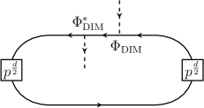
b)

c)

Figure 1: Three ways of looking at the same compactified network of intertwiners. a) Compactified network representing the trace of two Higgsed intertwiners $\Phi$ and $\Phi^{*}$ of the trigonometric DIM algebra. Wavy lines are identified so that the network lives on a cylinder. The solid horizontal line denotes the Fock representation $\mathcal{F}^{(1,0)}_{q,t^{-1}}$, while the vertical dashed lines are vector representations $\mathcal{V}_{q}$. $p$ plays the role of the circumference of the compactification circle; accordingly, $p^{d}$ is the box-counting operator. b) The same network as in a) drawn on a plane by projecting the cylinder. The box counting operator is split in two and the diagram ends with ‘‘cap’’ states on the left and right. c) The same intertwiner as in a) and b) written in terms of the elliptic DIM algebra with parameter $p$. In this description the ‘‘cap’’ states at the ends of the network correspond to vacuum states $\langle\varnothing|$ and $|\varnothing\rangle$ in the r.h.s. of Eq. (33). The horizontal line corresponds to the distinguished ‘‘double’’ Fock representation, and vertical dashed lines are vector representations of the elliptic DIM algebra.

After the compactification we want to keep the rule that a leg in the diagram corresponds to a representation of the algebra, but now the algebra is the elliptic DIM algebra. Its representations are non-isomorphic for different slopes $(n,m)$. Indeed, the slope corresponding to the direction of the compactification is distinguished. As we will see this representation is in fact a tensor product of two free boson Fock spaces, whereas the representation corresponding to the slope orthogonal to the direction of the compactification is a single Fock space. The reason for this doubling can be seen in Fig. 1. To reproduce the compactified diagram one needs to thread the compactified line two times and use special ‘‘cap’’ states on both ends. These states can be understood as the highest weight states of the horizontal Fock representation of the elliptic DIM algebra. We will consider the properties of these states in more detail in sec. 5.1.

We have collected the relevant facts about the elliptic DIM algebra and its representations in Appendix A. For a similar reference on the trigonometric DIM algebra we refer the reader to Appendix A of [17].

5.1 Thermo field double

In this section we summarize the theory of thermo field double and show how it can be used to get elliptic deformations of the Heisenberg algebra. In sec. 5.3 we apply this technique to the distinguished Heisenberg subalgebra of the elliptic DIM algebra and show that it can naturally be understood as a thermo field double of a Heisenberg subalgebra of trigonometric DIM algebra.

Consider a quantum system with Hilbert space $\mathcal{H}$ and Hamiltonian $H$. At nonzero temperature $\frac{1}{\beta}$ this system is described by the thermal density matrix

$$\rho_{\mathrm{therm}}=\frac{1}{Z(\beta)}e^{-\beta H},$$ (34)

where $Z(\beta)=\mathop{\mathrm{Tr}}\nolimits_{\mathcal{H}}e^{-\beta H}$. Thermal average of an operator $\mathcal{O}$ acting on $\mathcal{H}$ is computed by taking a trace with the density matrix:

$$\langle\mathcal{O}\rangle=\mathop{\mathrm{Tr}}\nolimits_{\mathcal{H}}(\rho_{\mathrm{therm}}\mathcal{O}).$$ (35)

If the temperature goes to zero, the trace in Eq. (35) becomes the vacuum matrix element:

$$\langle\mathcal{O}\rangle\stackrel{{\scriptstyle\beta\to+\infty}}{{\to}}\langle\mathrm{vac}|\mathcal{O}|\mathrm{vac}\rangle.$$ (36)

One can reformulate the theory in such a way that thermal averages of operators are also matrix elements (not traces). See e.g. [27] for an introduction to the technique. The price to pay is that all the degrees of freedom of the systems are doubled. Indeed, consider a state

$$|\Psi(\beta)\rangle=\frac{1}{\sqrt{Z(\beta)}}\sum_{n}e^{-\frac{\beta E_{n}}{2}}|n\rangle\otimes|n\rangle\in\mathcal{H}\otimes\mathcal{H},$$ (37)

where the sum runs over a complete orthonormal basis of states. We then identify the operator $\mathcal{O}$ with $\mathcal{O}\otimes 1$ and write

$$\langle\Psi(\beta)|\mathcal{O}|\Psi(\beta)\rangle=\frac{1}{Z(\beta)}\sum_{n}e^{-\beta E_{n}}\langle n|\mathcal{O}|n\rangle=\langle\mathcal{O}\rangle.$$ (38)

Thus, to compute thermal averages one can introduce a fictitious double of the system, and take matrix element between two judiciously chosen ‘‘thermal vacuum’’ states $|\Psi(\beta)\rangle$. Fig. 1 illustrates the reason why the doubling occurs: the Hilbert space $\mathcal{H}$ is ‘‘threaded two times’’ along the plane to reproduce the trace in (35).

It is remarkable, that for free fields the state $|\Psi(\beta)\rangle$ can in fact be obtained from the vacuum $|\mathrm{vac}\rangle\otimes|\mathrm{vac}\rangle$ by a Bogolyubov transformation.

5.1.1 Thermo-field double of a harmonic oscillator

Creation and annihilation operators $\tilde{a}$ and $\tilde{a}^{{\dagger}}$ act on $\mathcal{H}$ in the standard way, so that $[\tilde{a},\tilde{a}^{{\dagger}}]=1$ and $H=\tilde{a}^{{\dagger}}\tilde{a}$. Then $|\mathrm{vac}\rangle=|0\rangle$ and an orthonomral basis can be chosen as

$$|n\rangle=\frac{(\tilde{a}^{{\dagger}})^{n}}{\sqrt{n!}}|\varnothing\rangle.$$ (39)

We have

$$Z(\beta)=\sum_{n\geq 0}e^{-\beta n}=\frac{1}{1-e^{-\beta}}$$ (40)

and

$$|\Psi(\beta)\rangle=\sqrt{1-e^{-\beta}}\exp\left(e^{-\frac{\beta}{2}}\tilde{a}^{{\dagger}}_{(1)}\tilde{a}^{{\dagger}}_{(2)}\right)|\varnothing\rangle\otimes|\varnothing\rangle,$$ (41)

where $\tilde{a}^{{\dagger}}_{(1)}=a^{{\dagger}}\otimes 1$ and $a^{{\dagger}}_{(2)}=1\otimes\tilde{a}^{{\dagger}}$. The unitary Bogolyubov transformation from the vacuum state $|0\rangle\otimes|0\rangle$ to $|\Psi(\beta)\rangle$ is

$$U(\beta)=\exp\left(\theta(\tilde{a}^{{\dagger}}_{(1)}\tilde{a}^{{\dagger}}_{(2)}-\tilde{a}_{(1)}\tilde{a}_{(2)})\right),$$ (42)

where $\mathop{\mathrm{th}}\nolimits\theta=e^{-\frac{\beta}{2}}$. We give a short proof of this statement in Appendix B.

One can introduce the operators $a_{(1)}(\beta)$ and $a_{(2)}(\beta)$, which are Bogolyubov transformations of $a_{(1)}=a\otimes 1$ and $a_{(2)}=1\otimes a$:

$$\tilde{a}_{(i)}(\beta)=U(\beta)\tilde{a}_{(i)}U(\beta)^{-1}.$$ (43)

These ‘‘thermal’’ annihilation operators annihilate the thermal vacuum:

$$\tilde{a}_{(i)}(\beta)|\Psi(\beta)\rangle=0.$$ (44)

Of course, in a similar way the Bogolyubov transformation can be used to reexpress the original creation and annihilation operators $\tilde{a}=\tilde{a}_{(1)}$ and $\tilde{a}^{{\dagger}}=\tilde{a}_{(1)}^{{\dagger}}$ in terms of the new ‘‘thermal’’ operators $\tilde{a}_{(i)}(\beta)$, $\tilde{a}_{(i)}^{{\dagger}}(\beta)$:

$$\tilde{a} =\tilde{a}_{(1)}(\beta)\mathop{\mathrm{ch}}\nolimits\phi+\tilde{a}_{(2)}^{{\dagger}}(\beta)\mathop{\mathrm{sh}}\nolimits\phi=\frac{1}{\sqrt{1-e^{-\beta}}}(\tilde{a}_{(1)}(\beta)+\tilde{a}_{(2)}^{{\dagger}}(\beta)e^{-\beta/2}),$$ (45)

$$\tilde{a}^{{\dagger}} =\tilde{a}_{(1)}^{{\dagger}}(\beta)\mathop{\mathrm{ch}}\nolimits\phi+\tilde{a}_{(2)}(\beta)\mathop{\mathrm{sh}}\nolimits\phi=\frac{1}{\sqrt{1-e^{-\beta}}}(\tilde{a}_{(1)}^{{\dagger}}(\beta)+\tilde{a}_{(2)}(\beta)e^{-\beta/2}).$$ (46)

It will be convenient for us to rescale the ‘‘thermal’’ bosons introducing

$$a(\beta) =\sqrt{1-e^{-\beta}}\,\tilde{a}_{(1)}(\beta)=\tilde{a}_{(1)}+\tilde{a}_{(2)}^{{\dagger}}e^{-\beta/2},$$ (47)

$$b(\beta) =-e^{\beta/2}\sqrt{1-e^{-\beta}}\,\tilde{a}_{(2)}(\beta)=-e^{\beta/2}\tilde{a}_{(1)}^{{\dagger}}-\tilde{a}_{(2)},$$ (48)

so that the original generators $\tilde{a}$ are expressed through $a(\beta)$ and $b(\beta)$ as follows:

$$\tilde{a} =\frac{1}{1-e^{-\beta}}(a(\beta)-b^{{\dagger}}(\beta)e^{-\beta}),$$ (49)

$$\tilde{a}^{{\dagger}} =\frac{1}{1-e^{-\beta}}(a^{{\dagger}}(\beta)-b(\beta)e^{-\beta}).$$ (50)

The commutation relations for $a(\beta)$, $b(\beta)$ are:

$$[a(\beta),a^{{\dagger}}(\beta)]=1-e^{-\beta},\qquad[b(\beta),b^{{\dagger}}(\beta)]=e^{\beta}-1,\qquad[a(\beta),b^{{\dagger}}(\beta)]=[a(\beta),b(\beta)]=0.$$ (51)

In the low temperature limit $\beta\to+\infty$ the generators $a(\beta)$, $a^{{\dagger}}(\beta)$ turn into the original generators $\tilde{a}$, $\tilde{a}^{{\dagger}}$, while $b(\beta)$ and $b^{{\dagger}}(\beta)$ diverge and need to be rescaled by $e^{-\beta/2}$. After rescaling they give the decoupled thermal double generators $a_{(2)}$ and $a_{(2)}^{{\dagger}}$.

5.1.2 Thermo-field double of a Heisenberg algebra

Consider the Heisenberg algebra generated by the modes of the free chiral boson. The algebra is generated by $\tilde{a}_{n}$, $n\in\mathbb{Z}\backslash\{0\}$ and the zero modes $Q$ and $P$. The generators satisfy the commutation relations:

$$[\tilde{a}_{n},\tilde{a}_{m}]=n\delta_{n+m,0},\qquad[Q,P]=1,\qquad[\tilde{a}_{n},P]=[\tilde{a}_{n},Q]=0.$$ (52)

Each of the generators $\tilde{a}_{n}$ with $n>0$ is the annihilation operator of a harmonic oscillator, so the thermo-field double in this case is exactly the same as in sec. 5.1.1. The conjugate of $\tilde{a}_{n}$ in this setup is $\tilde{a}_{-n}$. Let us denote $e^{-\beta}=p$ from now on. We can again express the original generators $\tilde{a}_{n}$ in terms of the thermal generators $a_{n}(\beta)$ and $b_{n}(\beta)$ (for brevity we omit the argument $\beta$ henceforth):

$$\boxed{\tilde{a}_{n}=\frac{1}{1-p^{|n|}}(a_{n}-b_{-n}p^{|n|})}$$ (53)

where

$$[a_{n},a_{m}] =n(1-p^{|n|})\delta_{n+m,0},$$ (54)

$$[b_{n},b_{m}] =-n(1-p^{-|n|})\delta_{n+m,0},$$ (55)

$$[a_{n},b_{m}] =0.$$ (56)

The key aspect of introducing the new ‘‘thermal’’ bosons $a_{n}$ and $b_{n}$ is that one can now use the standard Wick’s theorem for them to compute the thermal correlators. Technically, this procedure works because the normal ordering for $a_{n}$ and $b_{n}$ differs form the normal ordering of the original operators $\tilde{a}_{n}$. The ‘‘new’’ normal ordering produces elliptic functions. Indeed, consider the free bosonic field

$$\tilde{\varphi}(z)=P\ln z+Q-\sum_{n\neq 0}\frac{1}{n}\tilde{a}_{n}z^{-n}.$$ (57)

One can build from it the standard primary field $V_{\alpha}(z)=:e^{\alpha\tilde{\varphi}(z)}:$, where the normal ordering is in terms of $\tilde{a}_{n}$. Let us rewrite $V_{\alpha}(z)$ in terms of $a_{n}$ and $b_{n}$ using Eq. (53):

$$V_{\alpha}(z)\sim e^{\alpha Q}z^{\alpha P}:\exp\left[-\alpha\sum_{n\neq 0}\frac{z^{-n}}{n(1-p^{|n|})}a_{n}\right]\exp\left[-\alpha\sum_{n\neq 0}\frac{p^{|n|}z^{n}}{n(1-p^{|n|})}b_{n}\right]:,$$ (58)

where the normal ordering is now in terms of $a_{n}$, $b_{n}$ (the reordering inside $V_{\alpha}(z)$ just rescales the vertex operator by a constant). Using Eqs. (54), (56) we get:

$$V_{\alpha_{1}}(z_{1})V_{\alpha_{2}}(z_{2})=:V_{\alpha_{1}}(z_{1})V_{\alpha_{2}}(z_{2}):z_{1}^{\alpha_{1}\alpha_{2}}\exp\left[-\alpha_{1}\alpha_{2}\sum_{n\geq 1}\frac{1}{n(1-p^{n})}\left[p^{n}\left(\frac{z_{1}}{z_{2}}\right)^{n}+\left(\frac{z_{2}}{z_{1}}\right)^{n}\right]\right]\sim\\ \sim:V_{\alpha_{1}}(z_{1})V_{\alpha_{2}}(z_{2}):z_{1}^{\alpha_{1}\alpha_{2}}\left(\theta_{p}\left(\frac{z_{2}}{z_{1}}\right)\right)^{\alpha_{1}\alpha_{2}}.$$ (59)

For elliptic DIM algebra we will use a similar rewriting of Heisenberg generators but in the opposite direction: we will be able to interpret all the elliptic functions in the elliptic DIM algebra commutation relations as arising from the ‘‘thermal’’ rewriting of a trigonometric DIM algebra plus an additional ‘‘thermal double’’ of its Heisenberg subalgebra.

5.2 Some hints on the structure of the elliptic DIM algebra

In this section we give some preliminary considerations which lead us to the understanding that the elliptic DIM algebra can be understood in terms of a thermo-field double of a trigonometric DIM algebra. To this end we look at the unrefined limit $t=q$ of the horizontal Fock representation $\mathcal{F}^{(1,0)}_{q,t^{-1}}$ of elliptic DIM algebra. The formulas for this representation are given in Appendix A.3.

In the unrefined limit the generating functions $\psi^{\pm}(z)$ tend to the identity and to get the nontrivial generators one needs to expand them in $(1-t/q)$ and keep the first order in the expansion. In this way we obtain:

$$x^{+}(z) =e^{P}:\exp\left[-\sum_{n\neq 0}\frac{1-q^{n}}{n(1-p^{|n|})}a_{n}z^{-n}\right]\exp\left[-\sum_{n\neq 0}\frac{1-q^{-n}}{n(1-p^{|n|})}b_{n}p^{|n|}z^{n}\right]:,$$ (60)

$$x^{-}(z) =e^{-P}:\exp\left[\sum_{n\neq 0}\frac{1-q^{n}}{n(1-p^{|n|})}a_{n}z^{-n}\right]\exp\left[\sum_{n\neq 0}\frac{1-q^{-n}}{n(1-p^{|n|})}b_{n}p^{|n|}z^{n}\right]:,$$ (61)

$$\psi^{+}(z) =1-(1-t/q)\left(\sum_{n\geq 1}\frac{(1-q^{n})}{(1-p^{n})}a_{n}z^{-n}+\sum_{n\geq 1}\frac{(1-q^{-n})p^{n}}{(1-p^{n})}b_{n}z^{n}\right),$$ (62)

$$\psi^{-}(z) =1+(1-t/q)\left(\sum_{n\geq 1}\frac{(1-q^{-n})}{(1-p^{n})}a_{-n}z^{n}-\sum_{n\geq 1}\frac{(1-q^{n})p^{n}}{(1-p^{n})}b_{-n}z^{-n}\right).$$ (63)

One can observe that the modes in the exponents in $x^{\pm}(z)$ (60), (61) combine precisely into (53), so that

$$x^{+}(z) \sim:\exp\left[-\sum_{n\neq 0}\frac{1-q^{n}}{n}\tilde{a}_{n}z^{-n}\right]:=:e^{\tilde{\varphi}(z)-\tilde{\varphi}(z/q)}:,$$ (64)

$$x^{-}(z) \sim:\exp\left[\sum_{n\neq 0}\frac{1-q^{n}}{n}\tilde{a}_{n}z^{-n}\right]:=:e^{-\tilde{\varphi}(z)+\tilde{\varphi}(z/q)}:,$$ (65)

where $\tilde{\varphi}(z)$ is the ‘‘non-thermal’’ free boson field (57).

The modes of $\psi^{\pm}(z)$ (62), (63), however, cannot be rewritten purely as functions of $a_{n}$. They depend not only on $a_{n}$ (i.e. $a_{n}\otimes 1=a_{n}^{(1)}$), but also on the second boson $a_{n}^{(2)}$ in the thermo-field double. This hints that the ‘‘vertical’’ Heisenberg subalgebra inside the elliptic DIM algebra generated by $\psi^{\pm}(z)$ is the doubled version of that of trigonometric DIM, whereas all other generators are just rewriting of the trigonometric expressions.

In the following section we demonstrate that the intuition that we have obtained for the restricted case of $t=q$ and horizontal Fock representation is in fact valid more generally. The elliptic DIM algebra with generic parameters can be explicitly written as a trigonometric DIM algebra plus a Heisenberg algebra without any reference to the choice of the representations.

5.3 Rewriting of the elliptic DIM algebra

In this section we show that by rewriting the basis of generators of the elliptic DIM algebra one can explicitly present it as a direct sum of a trigonometric DIM algebra and a Heisenberg algebra. Let us remind that the definitions and notations for elliptic DIM algebra are given in Appendix A.

5.3.1 Heisenberg subalgebras

It is evident that (for $\gamma\neq 1$) $H^{\pm}_{n}$ form two independent copies of the Heisenberg algebra. Indeed, two sets $\mathcal{A}_{\pm}=\{H^{\pm}_{n},H^{\mp}_{-n}|n>0\}$ commute between each other and each form a Heisenberg algebra. We would like to view these Heisenberg algebras as ‘‘thermal’’ bosons and perform the Bogolyubov transform akin to that described in sec. 5.1.2.

To this end we introduce the new basis of generators:

$$\boxed{\begin{aligned} \tilde{H}_{n}&=\operatorname{sgn}(n)(H^{+}_{n}-H^{-}_{n}),\\ \tilde{G}_{n}&=\operatorname{sgn}(n)(p^{-\frac{n}{2}}H^{+}_{-n}-p^{\frac{n}{2}}H^{-}_{-n}).\end{aligned}}$$ (66)

For convenience we also write down the inverse transformation between the bases:

$$H^{+}_{n} =\frac{\operatorname{sgn}(n)}{1-p^{n}}(\tilde{H}_{n}+p^{\frac{n}{2}}\tilde{G}_{-n}),$$ (67)

$$H^{-}_{n} =\frac{\operatorname{sgn}(n)p^{n}}{1-p^{n}}(\tilde{H}_{n}+p^{-\frac{n}{2}}\tilde{G}_{-n}).$$ (68)

The generators $\tilde{H}_{n}$ and $\tilde{G}_{n}$ also satisfy two independent copies of Heisenberg algebras, but now without any dependence on $p$:

$$[\tilde{H}_{n},\tilde{H}_{m}]=[\tilde{G}_{n},\tilde{G}_{m}]=\delta_{n+m,0}\frac{\kappa_{n}(\gamma^{n}-\gamma^{-n})}{n},$$ (69)

$$[\tilde{H}_{n},\tilde{G}_{m}]=0.$$ (70)

where $\kappa_{n}=(1-q^{n})(1-t^{-n})(1-t^{n}q^{-n})$. In what follows we show that the Heisenberg algebra generated by $\tilde{H}_{n}$ together with the dressed generators $\tilde{x}^{\pm}(z)$ in fact form a trigonometric DIM algebra, while the second Heisenberg algebra of $\tilde{G}_{n}$ decouples completely.

In view of this hypothesis we define the currents of the Heisenberg subalgebra of the (would be) trigonometric DIM algebra

$$\tilde{\psi}^{\pm}(z)=\exp\left[\sum_{n>0}\tilde{H}_{\pm n}z^{\mp n}\right],$$ (71)

and the decoupled Heisenberg currents

$$\tilde{\phi}^{\pm}(z)=\exp\left[\sum_{n>0}\tilde{G}_{\pm n}z^{\mp n}\right].$$ (72)

5.3.2 Dressing factors

Beyond the vertical Heisenberg subalgebras formed by $H^{\pm}_{n}$ we have to modify the generating currents $x^{\pm}(z)$. Indeed, in elliptic DIM algebra $x^{+}(z)$ satisfy the commutation relations with elliptic structure functions $G^{\pm}_{p}(x)$, while the trigonometric algebra features the trigonometric structure function

$$G^{\pm}(x)=G^{\pm}_{p=0}(x)=(1-q^{\pm 1}x)(1-t^{\mp 1}x)(1-t^{\pm 1}q^{\mp 1}x).$$ (73)

We introduce two dressing factors:

$$\Gamma_{H}(z) =\exp\left[-\sum_{n\neq 0}\frac{p^{|n|}}{(1-p^{|n|})(\gamma^{\frac{n}{2}}+\gamma^{-\frac{n}{2}})}\tilde{H}_{n}z^{-n}\right],$$ (74)

$$\Gamma_{G}(z) =\exp\left[-\sum_{n\neq 0}\frac{p^{|n|}}{(1-p^{|n|})(\gamma^{\frac{n}{2}}+\gamma^{-\frac{n}{2}})}p^{-\frac{|n|}{2}}\tilde{G}_{n}z^{n}\right].$$ (75)

Using the factors (74), (75) we define the dressed currents as follows

$$\tilde{x}^{\pm}(z)=c_{\pm}x^{\pm}(z)\Gamma_{H}(z)\Gamma_{G}(z)=x^{\pm}(z)\exp\left[-\sum_{n\neq 0}\frac{p^{|n|}}{(1-p^{|n|})(\gamma^{\frac{n}{2}}+\gamma^{-\frac{n}{2}})}\left(\tilde{H}_{n}+p^{-\frac{|n|}{2}}\tilde{G}_{-n}\right)z^{-n}\right],$$ (76)

where the constants $c_{\pm}$ are chosen so that

$$c_{+}c_{-}=\frac{G_{p}^{-}(1)}{(p;p)_{\infty}^{3}G_{0}^{-}(1)}\exp\left[\sum_{n\geq 1}\frac{\kappa_{n}}{n}\frac{p^{n}(1-\gamma^{n})}{1-p^{n}}\right],$$ (77)

where $G_{p}^{\pm}(x)$ is defined in Eq. (102). The renormalization constants $c_{\pm}$ depend on the particular way we order the dressing factors. Their job is to ensure that the commutation relation (100) holds with correct prefactor in front of the right hand side.

The dressed currents can also be expressed through the old generators $H^{\pm}_{n}$:

$$\boxed{\tilde{x}^{\pm}(z)=x^{\pm}(z)\exp\left[-\sum_{n\neq 0}\frac{H^{-\operatorname{sgn}(n)}_{n}z^{-n}}{\gamma^{\frac{n}{2}}+\gamma^{-\frac{n}{2}}}\right]}$$ (78)

In this way we can clearly see that in the limit $p\to 0$ the dressing factors become trivial, since they depend on the generators $H^{+}_{n<0}$ and $H^{-}_{n>0}$ which vanish in this limit (see Appendix A.1). They also trivialize for $t=q$ because in that case $H_{n}^{-\operatorname{sgn}(n)}\sim(1-t/q)\to 0$.

The dressing factors $\Gamma_{H}(z)$, $\Gamma_{G}(z)$ enjoy the following commutation relations between themselves and the currents $\tilde{x}^{\pm}(z)$:

$$[\Gamma_{H}(z),\Gamma_{G}(w)]=[\tilde{x}^{\pm}(z),\Gamma_{G}(z)]=0,$$ (79)

$$\Gamma_{H}(z)\Gamma_{H}(w)=\exp\left[\sum_{n\neq 0}\frac{\kappa_{n}}{n}\left(\frac{w}{z}\right)^{n}\frac{p^{2|n|}}{(1-p^{|n|})^{2}}\frac{\gamma^{\frac{n}{2}}-\gamma^{-\frac{n}{2}}}{\gamma^{\frac{n}{2}}+\gamma^{-\frac{n}{2}}}\right]\Gamma_{H}(w)\Gamma_{H}(z),$$ (80)

$$\Gamma_{G}(z)\Gamma_{G}(w)=\exp\left[-\sum_{n\neq 0}\frac{\kappa_{n}}{n}\left(\frac{w}{z}\right)^{n}\frac{p^{|n|}}{(1-p^{|n|})^{2}}\frac{\gamma^{\frac{n}{2}}-\gamma^{-\frac{n}{2}}}{\gamma^{\frac{n}{2}}+\gamma^{-\frac{n}{2}}}\right]\Gamma_{G}(w)\Gamma_{G}(z),$$ (81)

$$\Gamma_{H}(z)\tilde{x}^{\pm}(w)=\exp\left[\pm\sum_{n\neq 0}\operatorname{sgn}(n)\frac{\kappa_{n}}{n}\left(\frac{w}{z}\right)^{n}\frac{p^{|n|}\gamma^{\mp\frac{|n|}{2}}}{1-p^{|n|}}\frac{1}{\gamma^{\frac{n}{2}}+\gamma^{-\frac{n}{2}}}\right]\tilde{x}^{\pm}(w)\Gamma_{H}(z).$$ (82)

Using the relations (79)–(82) it is straightforward to check that the dressed currents obey the ordinary (i.e. trigonometric) DIM algebra, while the currents $\tilde{\phi}^{\pm}(z)$ decouple:

$$[\tilde{\phi}^{\pm}(z),\tilde{\psi}^{+}(w)]=[\tilde{\phi}^{\pm}(z),\tilde{\psi}^{-}(w)]=[\tilde{\phi}^{\pm}(z),\tilde{x}^{+}(w)]=[\tilde{\phi}^{\pm}(z),\tilde{x}^{-}(w)]=0,$$ (83)

$$[\tilde{\psi}^{\pm}(z),\tilde{\psi}^{\pm}(w)]=0,\qquad\tilde{\psi}^{+}(z)\tilde{\psi}^{-}(w)=\frac{g_{0}\left(\gamma\frac{w}{z}\right)}{g_{p}\left(\gamma^{-1}\frac{w}{z}\right)}\tilde{\psi}^{-}(w)\tilde{\psi}^{+}(z),$$ (84)

$$\tilde{\psi}^{+}(z)\tilde{x}^{\pm}(w)=g_{0}\left(\gamma^{\mp\frac{1}{2}}\frac{w}{z}\right)^{\mp 1}\tilde{x}^{\pm}(w)\tilde{\psi}^{+}(z),\qquad\tilde{\psi}^{-}(z)\tilde{x}^{\pm}(w)=g_{0}\left(\gamma^{\mp\frac{1}{2}}\frac{w}{z}\right)^{\pm 1}\tilde{x}^{\pm}(w)\tilde{\psi}^{-}(z),$$ (85)

$$[\tilde{x}^{+}(z),\tilde{x}^{-}(w)]=\frac{1}{G_{0}^{-}(1)}\left(\delta\left(\gamma^{-1}\frac{z}{w}\right)\tilde{\psi}^{+}\left(\gamma^{\frac{1}{2}}w\right)-\delta\left(\gamma\frac{z}{w}\right)\tilde{\psi}^{-}\left(\gamma^{-\frac{1}{2}}w\right)\right),$$ (86)

$$G_{0}^{\mp}\left(\frac{z}{w}\right)\tilde{x}^{\pm}(z)\tilde{x}^{\pm}(w)=G_{0}^{\pm}\left(\frac{z}{w}\right)\tilde{x}^{\pm}(w)\tilde{x}^{\pm}(z).$$ (87)

Notice that $p$ does not enter the relations (83)–(87). In this sense the elliptic deformation of the DIM algebra is superficial: it can be reproduced by adding a Heisenberg algebra to the undeformed DIM algebra and then relabelling the generators.

5.3.3 Twisting the coproduct and the elliptic $R$-matrix

In sec. 5.3.2 we have proven the isomorphism of two algebras: the elliptic DIM algebra and the trigonometric DIM algebra plus a Heisenberg algebra. However, the algebras on both sides of the equivalence are in fact Hopf algebras, so it is natural to ask how their coproduct structures are related. Here the situation is more subtle, because the standard coproduct structure (111)–(114) on the elliptic DIM algebra does not coincide with the standard coproduct on the trigonometric DIM algebra. For example, we have

$$\Delta_{\mathrm{ell}}(H_{n}^{\pm}) =H^{\pm}_{n}\otimes\gamma^{\mp\frac{n}{2}}+\gamma^{\pm\frac{n}{2}}\otimes H^{\pm}_{n},$$ (88)

$$\Delta_{\mathrm{trig}}(H_{n}^{\pm}) =H^{\pm}_{n}\otimes\gamma^{-\frac{|n|}{2}}+\gamma^{\frac{|n|}{2}}\otimes H^{\pm}_{n},$$ (89)

where $\Delta_{\mathrm{ell}}$ denotes the coproduct (111)–(114) on elliptic DIM, and $\Delta_{\mathrm{trig}}$ is the coproduct obtained from the standard coproduct on the trigonometric DIM algebra after the change of variables (66). As one can see the Eq. (88) and Eq. (89) are manifestly different.

However, we conjecture that the two coproducts $\Delta_{\mathrm{ell}}$ and $\Delta_{\mathrm{trig}}$ are related by a nontrivial Drinfeld twist $F$, so that the coalgebraic structures on elliptic and trigonometric DIM algebras are isomorphic. We have not been able to obtain an explicit expression for $F$, but we think that it can be written in Khoroshkin-Tolstoy form as an (infinite) product of elementary twists, the first of which is

$$F=\exp\left[-\sum_{n\geq 1}\frac{n}{\kappa_{n}}(1-p^{-n})\gamma^{\frac{n}{2}}H^{+}_{-n}\otimes\gamma^{-\frac{n}{2}}H^{-}_{n}\right]\times\cdots$$ (90)

and all other factors lie in the Heisenberg subalgebras with nonvertical ‘‘slope’’ inside the elliptic DIM algebra.

Using the expression (90), incomplete as it is, we can still find the elliptic $R$-matrix in a tensor product of two vertical vector representations $\mathcal{V}_{q}$. To this end we recall that the $R$-matrix after the Drinfeld twist is given by

$$R_{\mathrm{ell}}=FR_{\mathrm{trig}}F_{\mathrm{op}}^{-1},$$ (91)

where $F_{\mathrm{op}}$ denotes $F$ with the two tensor factors exchanged. We also notice that all the terms denoted by $\cdots$ in Eq. (90) do not contribute to the $R$-matrix in the vertical representations, which turns out to be diagonal. Using Eq. (127), (128) we then find

$$F|_{\mathcal{V}_{q}\otimes\mathcal{V}_{q}}|f(x_{1},x_{2})\rangle=\exp\left[\sum_{n\geq 1}\frac{1}{n}\left(\frac{x_{2}}{x_{1}}\right)^{n}\frac{(1-t^{n})(1-(q/t)^{n})p^{n}}{(1-p^{n})(1-q^{n})}\right]|f(x_{1},x_{2})\rangle=\\ =\frac{\left(pt\frac{x_{2}}{x_{1}};q,p\right)_{\infty}\left(\frac{pq}{t}\frac{x_{2}}{x_{1}};q,p\right)_{\infty}}{\left(p\frac{x_{2}}{x_{1}};q,p\right)_{\infty}\left(pq\frac{x_{2}}{x_{1}};q,p\right)_{\infty}}|f(x_{1},x_{2})\rangle,$$ (92)

and

$$(F_{\mathrm{op}})^{-1}|_{\mathcal{V}_{q}\otimes\mathcal{V}_{q}}|f(x_{1},x_{2})\rangle=\frac{\left(p\frac{x_{1}}{x_{2}};q,p\right)_{\infty}\left(pq\frac{x_{1}}{x_{2}};q,p\right)_{\infty}}{\left(pt\frac{x_{1}}{x_{2}};q,p\right)_{\infty}\left(\frac{pq}{t}\frac{x_{1}}{x_{2}};q,p\right)_{\infty}}|f(x_{1},x_{2})\rangle,$$ (93)

where

$$(x;q,p)_{\infty}=\prod_{i,j\geq 0}(1-q^{i}p^{j}x).$$ (94)

Using the expression for the trigonometric $R$-matrix from [17]

$$R_{\mathrm{trig}}|_{\mathcal{V}_{q}\otimes\mathcal{V}_{q}}|f(x_{1},x_{2})\rangle=\frac{\left(\frac{x_{1}}{x_{2}};q\right)_{\infty}\left(q\frac{x_{1}}{x_{2}};q\right)_{\infty}}{\left(\frac{qx_{1}}{tx_{2}};q\right)_{\infty}\left(t\frac{x_{1}}{x_{2}};q\right)_{\infty}}|f(x_{1},x_{2})\rangle$$ (95)

we get:

$$R_{\mathrm{ell}}|_{\mathcal{V}_{q}\otimes\mathcal{V}_{q}}|f(x_{1},x_{2})\rangle=\frac{\Gamma_{q,p}\left(\frac{qx_{1}}{tx_{2}}\right)\Gamma_{q,p}\left(t\frac{x_{1}}{x_{2}}\right)}{\Gamma_{q,p}\left(\frac{x_{1}}{x_{2}}\right)\Gamma_{q,p}\left(q\frac{x_{1}}{x_{2}}\right)}|f(x_{1},x_{2})\rangle,$$ (96)

where

$$\Gamma_{q,p}(x)=\frac{\left(\frac{qp}{x};q,p\right)_{\infty}}{(x;q,p)_{\infty}}.$$ (97)

This coincides with the $R$-matrix obtained from the commutation of the intertwiners.

6 Conclusions and discussions

In the first part of the paper we have studied the elliptic uplift of higgsed networks of intertwiners using two different approaches: either by deforming the DIM algebra and the intertwiners, or by compactifying the network. We have found the commutation relations of the elliptically deformed intertwiners and evaluated elliptic correlators, which reproduce partition functions of $4d$ linear quiver gauge theories compactified on a two-dimensional torus $T^{2}$. We have found that the two approaches give essentially the same partition functions up to some prefactors associated with flavour symmetries. These prefactors cancel out when two linear quivers are glued together and a flavour symmetry subgroup is gauged. We have found that the elliptic uplifts of the higgsed intertwiners are in fact the intertwiners of the elliptic deformation of DIM algebra introduced in [18].

In the second more abstract part of the paper we have investigated elliptic DIM algebra itself. Using a dressing transformation of the generating currents we have found a remarkable isomorphism between elliptic DIM algebra and a direct sum of two simpler algebras: the undeformed DIM algebra and the Heisenberg algebra. We have also conjectured that the isomorphism of the algebras extends to an isomorphism of Hopf algebras and have partly determined the corresponding Drinfeld twist.

DIM algebra has a $\mathbb{Z}^{2}$ worth of generators with $SL(2,\mathbb{Z})$ automorphism group acting on them in a standard way. Elliptic deformation is not invariant under the $SL(2,\mathbb{Z})$ transformations, since it depends on the choice of the compactification direction (or, according to the isomorphism described in the previous paragraph, on the slope of the ‘‘extra’’ Heisenberg algebra added to the DIM algebra). However, DIM algebra before the deformation already possessed a preferred direction, which is encoded in the choice of the coalgebra structure, i.e. the coproduct. Different choices of the coproduct on DIM lagebra are all related to each other by $SL(2,\mathbb{Z})$ transformations. However, after the deformation there appear to be two distinguished directions in the setup: the preferred direction and the direction of the compactification. Though they both can be rotated by $SL(2,\mathbb{Z})$, their relative slope remains invariant. It would be interesting to understand if this non-invariance is essential or can be undone with a cleverly chosen Drinfeld twist. Another question to ask is what happens if one doubly compactifies the theory. Naively this should restore (or even enhance) the $SL(2,\mathbb{Z})$ symmetry. However, this remains to be seen.

It is also natural to consider higgsed networks compacitified not along the horizontal but along the vertical direction. They should give rise to $3d$ circular quiver gauge theories. One can ask if these theories are related to the ‘‘horizontally compactified’’ $4d$ theories that we have considered here. We can then hypothesize that there are two ways to deform the DIM algebra: the elliptic one and the (still missing) affine one. It is possible that there is a corresponding relation between these two deformations obtained by compactifying along two orthogonal directions.

7 Acknowledgements

We are grateful to A. Morozov, A. Mironov and S. Mironov for discussions. Y.Z. is partly supported by RFBR grants 19-51-50008-YaF, 19-51-18006-Bolg and 21-52-52004-MNT.

Appendix A Elliptic DIM algebra and some of its representations

In this appendix we write out the definition of the elliptic DIM algebra $U_{q,t,p}^{\mathrm{ell}}(\widehat{\widehat{\mathfrak{gl}}}_{1})$, its coalgebra structure and two types of representations relevant for us — the horizontal Fock representation and the vector representation.

A.1 Elliptic DIM algebra

The algebra $U_{q,t,p}^{\mathrm{ell}}(\widehat{\widehat{\mathfrak{gl}}}_{1})$ is generated by the currents $x^{\pm}(z)=\sum_{n\in\mathbb{Z}}x^{\pm}_{n}z^{-n}$, $\psi^{\pm}(z)=\sum_{n\in\mathbb{Z}}\psi^{\pm}_{n}z^{-n}$ and a central element $\gamma$ satisfying the relations [18]

$$[\psi^{\pm}(z),\psi^{\pm}(w)]=0,\qquad\psi^{+}(z)\psi^{-}(w)=\frac{g_{p}\left(\gamma\frac{w}{z}\right)}{g_{p}\left(\gamma^{-1}\frac{w}{z}\right)}\psi^{-}(w)\psi^{+}(z),$$ (98)

$$\psi^{+}(z)x^{\pm}(w)=g_{p}\left(\gamma^{\mp\frac{1}{2}}\frac{w}{z}\right)^{\mp 1}x^{\pm}(w)\psi^{+}(z),\qquad\psi^{-}(z)x^{\pm}(w)=g_{p}\left(\gamma^{\mp\frac{1}{2}}\frac{w}{z}\right)^{\pm 1}x^{\pm}(w)\psi^{-}(z),$$ (99)

$$[x^{+}(z),x^{-}(w)]=\frac{(p;p)_{\infty}^{3}}{G_{p}^{-}(1)}\left(\delta\left(\gamma^{-1}\frac{z}{w}\right)\psi^{+}\left(\gamma^{\frac{1}{2}}w\right)-\delta\left(\gamma\frac{z}{w}\right)\psi^{-}\left(\gamma^{-\frac{1}{2}}w\right)\right),$$ (100)

$$G_{p}^{\mp}\left(\frac{z}{w}\right)x^{\pm}(z)x^{\pm}(w)=G_{p}^{\pm}\left(\frac{z}{w}\right)x^{\pm}(w)x^{\pm}(z),$$ (101)

where $\delta(x)=\sum_{n\in\mathbb{Z}}x^{n}$ and the ‘‘structure functions’’ of the algebra are elliptic deformations of the ordinary DIM structure functions given by

$$G_{p}^{\pm}(x)=\theta_{p}(q^{\pm 1}x)\theta_{p}(t^{\mp 1}x)\theta_{p}(t^{\pm 1}q^{\mp 1}x),\qquad\theta_{p}(x)=(p;p)_{\infty}(x;p)_{\infty}(p/x;p)_{\infty},$$ (102)

$$g(x)=\frac{G_{p}^{+}(x)}{G_{p}^{-}(x)}.$$ (103)

The structure function satisfies $g_{p}\left(\frac{1}{x}\right)=\frac{1}{g_{p}(x)}$ and in particular $g_{p}(1)=-1$ so that $G_{p}^{+}(1)=-G_{p}^{-}(1)$. Notice that in contrast to the trigonometric case there are both positive and negative modes in the currents $\psi^{\pm}(z)$. Just as the trigonometric DIM algebra, the elliptic one is manifestly symmetric under any permutation of the parameters $q$, $t^{-1}$, and $\frac{t}{q}$.

In the limit $p\to 0$ elliptic structure function turns into trigonometric one:

$$G^{\pm}(x)\stackrel{{\scriptstyle p\to 0}}{{\to}}(1-q^{\pm 1}x)(1-t^{\mp 1}x)(1-t^{\pm 1}q^{\mp 1}x),$$ (104)

so that the conventional DIM algebra is recovered.

It is convenient to introduce the generators $H^{\pm}_{n}$ such that

$$\psi^{\pm}(z)=\psi^{\pm}_{0}\exp\left[\sum_{n\neq 0}H^{\pm}_{n}z^{-n}\right].$$ (105)

The elements $\psi^{\pm}_{0}$ are central. Notice that, unlike the trigonometric case the index $n\neq 0$ can be both positive and negative for $H^{\pm}_{n}$. We can rewrite the commutation relations (98)–(99) in terms of $H_{n}^{\pm}$:

$$[H^{\pm}_{n},H^{\pm}_{m}]=0,\qquad\qquad[H^{+}_{n},H^{-}_{m}]=\delta_{n+m,0}\frac{\kappa_{n}}{n(1-p^{n})}(\gamma^{n}-\gamma^{-n}),$$ (106)

$$[H^{+}_{n},x^{\pm}(z)]=\mp\frac{\kappa_{n}}{n(1-p^{n})}\gamma^{\mp\frac{n}{2}}z^{n}x^{\pm}(z),$$ (107)

$$[H^{-}_{n},x^{\pm}(z)]=\mp\frac{\kappa_{n}p^{n}}{n(1-p^{n})}\gamma^{\pm\frac{n}{2}}z^{n}x^{\pm}(z).$$ (108)

where $\kappa_{n}=(1-q^{n})(1-t^{-n})(1-t^{n}q^{-n})=-\kappa_{-n}$. In the limit $p\to 0$ the fate of the generators $H^{\pm}_{n}$ can be read from the commutation relations (106) and depends on the sign of the index $n$:

1. $H^{+}_{n>0}$ and $H^{-}_{n<0}$ remain finite and become the modes of the ‘‘vertical’’ Heisenberg subalgebra of the trigonometric DIM algebra.

2. $H^{+}_{n<0}$ and $H^{-}_{n>0}$ vanish as $\sqrt{p}$ in the $p\to 0$ limit. Naively, they disappear completely so that only half of the ‘‘elliptic’’ modes $H^{\pm}_{n}$ remain in the trigonometric limit. However, if one rescales the vanishing modes by $p^{-1/2}$ they survive and form an extra Heisenberg algebra. See sec. 5.3.1 for the complete description of this Heisenberg subalgebra valid for general $p$.

In writing Eqs. (106)–(108) one has to be careful, since there are two ways to write the structure function $g_{p}(x)$ as an exponential (they differ by an infinite sum of delta-functions):

$$g_{p}(x)=\exp\left[\sum_{n\neq 0}\frac{\kappa_{n}}{n}\frac{x^{n}}{1-p^{n}}\right],$$ (109)

or

$$(g_{p}(x^{-1}))^{-1}=\exp\left[\sum_{n\neq 0}\frac{\kappa_{n}}{n}\frac{p^{n}x^{n}}{1-p^{n}}\right].$$ (110)

To determine which one is needed in each commutation relation one can check the limit $p\to 0$. According to Eq. (106)

There exists a coproduct on the elliptic DIM algebra given by:

$$\Delta(\gamma) =\gamma\otimes\gamma,$$ (111)

$$\Delta(\psi^{\pm}(z)) =\psi^{\pm}(\gamma_{(2)}^{\pm\frac{1}{2}}z)\otimes\psi^{\pm}(\gamma_{(1)}^{\mp\frac{1}{2}}z),$$ (112)

$$\Delta(x^{+}(z)) =x^{+}(z)\otimes 1+\psi^{-}(\gamma_{(1)}^{\frac{1}{2}}z)\otimes x^{+}(\gamma_{(1)}z),$$ (113)

$$\Delta(x^{-}(z)) =x^{-}(\gamma_{(2)}z)\otimes\psi^{+}(\gamma_{(2)}^{\frac{1}{2}}z)+1\otimes x^{-}(z),$$ (114)

where $\gamma_{(1)}=\gamma\otimes 1$ and $\gamma_{(2)}=1\otimes\gamma$. In terms of the generators $H_{n}^{\pm}$ the coproduct (112) reads

$$\Delta(H_{n}^{\pm})=H^{\pm}_{n}\otimes\gamma^{\mp\frac{n}{2}}+\gamma^{\pm\frac{n}{2}}\otimes H_{n}^{\pm}.$$ (115)

For completeness let us also give the expressions for the counit $\epsilon$

$$\epsilon(x^{\pm}(z))=\epsilon(H_{n}^{\pm})=0,$$ (116)

$$\epsilon(\gamma)=\epsilon(\psi^{\pm}_{0})=1.$$ (117)

and (formal) antipode $S$ of the elliptic DIM algebra:

$$S(\gamma) =\gamma^{-1},$$ (118)

$$S(\psi^{\pm}(z)) =(\psi^{\pm}(z))^{-1},$$ (119)

$$S(x^{+}(z)) =-\left(\psi^{-}(\gamma^{-\frac{1}{2}}z)\right)^{-1}x^{+}(\gamma^{-1}z),$$ (120)

$$S(x^{-}(z)) =-x^{-}(\gamma^{-1}z)\left(\psi^{+}(\gamma^{-\frac{1}{2}}z)\right)^{-1}.$$ (121)

A.2 Vector representation

Vector representation $\mathcal{V}_{q}$ is the representation of the elliptic DIM with trivial central charges on the space of functions [26].

$$x^{+}(z)f(x) =-\frac{1}{\theta_{p}(q^{-1})}\delta\left(\frac{x}{qz}\right)q^{-x\partial_{x}}f(x),$$ (122)

$$x^{-}(z)f(x) =-\frac{1}{\theta_{p}(q)}\delta\left(\frac{x}{z}\right)q^{x\partial_{x}}f(x),$$ (123)

$$\psi^{+}(z)f(x) =\frac{\theta_{p}\left(\frac{tx}{qz}\right)\theta_{p}\left(\frac{x}{tz}\right)}{\theta_{p}\left(\frac{x}{z}\right)\theta_{p}\left(\frac{x}{qz}\right)}f(x),$$ (124)

$$\psi^{-}(z)f(x) =\frac{\theta_{p}\left(\frac{qz}{tx}\right)\theta_{p}\left(\frac{tz}{x}\right)}{\theta_{p}\left(\frac{z}{x}\right)\theta_{p}\left(q\frac{z}{x}\right)}f(x),$$ (125)

$$\gamma f(x) =f(x).$$ (126)

There are three vector representations obtained by exchanging $q\to t^{-1}\to\frac{t}{q}$. In terms of $H^{\pm}_{n}$ generators we have

$$H_{n}^{+}f(x) =\frac{x^{n}(1-t^{-n})\left(1-\left(\frac{t}{q}\right)^{n}\right)}{n(1-p^{n})}f(x),$$ (127)

$$H_{n}^{-}f(x) =\frac{x^{n}p^{n}(1-t^{-n})\left(1-\left(\frac{t}{q}\right)^{n}\right)}{n(1-p^{n})}f(x).$$ (128)

A.3 Horizontal Fock representation

In this representation $\mathcal{F}_{t^{-1},t/q}$ [18] DIM algebra acts on the tensor product of two free boson Fock spaces generated by the modes $a_{n}$ and $b_{n}$ satisfying the commutation relations

$$[a_{n},a_{m}] =n\delta_{n+m,0}(1-p^{|n|})\frac{1-q^{|n|}}{1-t^{|n|}},$$ (129)

$$[b_{n},b_{m}] =-n\delta_{n+m,0}(1-p^{-|n|})\frac{1-q^{-|n|}}{1-t^{-|n|}},$$ (130)

$$[a_{n},b_{m}] =0.$$ (131)

We also introduce the zero modes $Q$ and $P$ commuting with $a_{n}$ and $b_{n}$ and satisfying

$$[P,Q]=1.$$ (132)

$P$ acts diagonally on $\mathcal{F}_{t^{-1},t/q}$ and gives the spectral parameters of the Fock representation:

$$e^{P}|_{\mathcal{F}_{t^{-1},t/q}(u)}=u.$$ (133)

The operator $Q$ acts between different Fock representations by shifting the spectral parameter. We use it in the intertwiner

The elliptic DIM algebra generators act as follows:

$$x^{+}(z) =\frac{(p;p)_{\infty}^{3}e^{P}}{\theta_{p}(q^{-1})\theta_{p}(t)}:\exp\left[-\sum_{n\neq 0}\frac{1-t^{n}}{n(1-p^{|n|})}a_{n}z^{-n}\right]\exp\left[-\sum_{n\neq 0}\frac{1-t^{-n}}{n(1-p^{|n|})}b_{n}p^{|n|}z^{n}\right]:,$$ (134)

$$x^{-}(z) =\frac{(p;p)_{\infty}^{3}e^{-P}}{\theta_{p}(q^{-1})\theta_{p}(t^{-1})}:\exp\left[\sum_{n\neq 0}\left(\frac{t}{q}\right)^{\frac{|n|}{2}}\frac{1-t^{n}}{n(1-p^{|n|})}a_{n}z^{-n}\right]\exp\left[\sum_{n\neq 0}\left(\frac{t}{q}\right)^{-\frac{|n|}{2}}\frac{1-t^{-n}}{n(1-p^{|n|})}b_{n}p^{|n|}z^{n}\right]:,$$ (135)

$$\psi^{+}(z) =\exp\left[-\sum_{n\geq 1}\frac{(1-t^{n})(1-t^{n}/q^{n})}{n(1-p^{n})}\left(\frac{q}{t}\right)^{\frac{n}{4}}a_{n}z^{-n}\right]\exp\left[-\sum_{n\geq 1}\frac{(1-t^{-n})(1-q^{n}/t^{n})p^{n}}{n(1-p^{n})}\left(\frac{t}{q}\right)^{\frac{n}{4}}b_{n}z^{n}\right],$$ (136)

$$\psi^{-}(z) =\exp\left[\sum_{n\geq 1}\frac{(1-t^{-n})(1-t^{n}/q^{n})}{n(1-p^{n})}\left(\frac{q}{t}\right)^{\frac{n}{4}}a_{-n}z^{n}\right]\exp\left[\sum_{n\geq 1}\frac{(1-t^{n})(1-q^{n}/t^{n})p^{n}}{n(1-p^{n})}\left(\frac{t}{q}\right)^{\frac{n}{4}}b_{-n}z^{-n}\right],$$ (137)

$$\gamma =\sqrt{\frac{t}{q}},$$ (138)

or, in terms of $H^{\pm}_{n}$ generators:

$$H^{+}_{n} =-\frac{(1-t^{n})\left(1-\left(\frac{t}{q}\right)^{n}\right)}{n(1-p^{n})}\left(\frac{q}{t}\right)^{\frac{n}{4}}\begin{cases}a_{n},&n>0,\\ b_{-n},&n<0,\end{cases}$$ (139)

$$H^{-}_{n} =-\frac{(1-t^{n})\left(1-\left(\frac{q}{t}\right)^{n}\right)}{n(1-p^{-n})}\left(\frac{t}{q}\right)^{\frac{n}{4}}\begin{cases}b_{-n},&n>0,\\ a_{n},&n<0.\end{cases}$$ (140)

Appendix B Thermo-field double as a Bogolyubov transformation

Let us prove that the thermo-field vacuum state (41) can be obtained from the standard vacuum $|0\rangle\otimes|0\rangle$ by the Bogolyubov transformation (42). Indeed, we notice that

$$(a^{{\dagger}}_{(1)}a^{{\dagger}}_{(2)}-a_{(1)}a_{(2)})e^{\psi a^{{\dagger}}_{(1)}a^{{\dagger}}_{(2)}}|\varnothing\rangle\otimes|\varnothing\rangle=\left((1-\psi^{2})\frac{\partial}{\partial\psi}-\psi\right)e^{\psi a^{{\dagger}}_{(1)}a^{{\dagger}}_{(2)}}|\varnothing\rangle\otimes|\varnothing\rangle.$$ (141)

We introduce the new coordinate $\phi(\psi)$ such that

$$(1-\psi^{2})\frac{\partial}{\partial\psi}=\frac{\partial}{\partial\phi},$$ (142)

and therefore

$$\psi(\phi)=\mathop{\mathrm{th}}\nolimits\phi.$$ (143)

We have

$$(a^{{\dagger}}_{(1)}a^{{\dagger}}_{(2)}-a_{(1)}a_{(2)})e^{\psi a^{{\dagger}}_{(1)}a^{{\dagger}}_{(2)}}|\varnothing\rangle\otimes|\varnothing\rangle=\left(\frac{\partial}{\partial\phi}-\mathop{\mathrm{th}}\nolimits\phi\right)e^{\mathop{\mathrm{th}}\nolimits(\phi)a^{{\dagger}}_{(1)}a^{{\dagger}}_{(2)}}|\varnothing\rangle\otimes|\varnothing\rangle=\\ =\mathop{\mathrm{ch}}\nolimits(\phi)\frac{\partial}{\partial\phi}\left[\frac{1}{\mathop{\mathrm{ch}}\nolimits\phi}e^{\mathop{\mathrm{th}}\nolimits(\phi)a^{{\dagger}}_{(1)}a^{{\dagger}}_{(2)}}|0\rangle\otimes|0\rangle\right],$$ (144)

So that

$$\exp(\theta(a^{{\dagger}}_{(1)}a^{{\dagger}}_{(2)}-a_{(1)}a_{(2)}))e^{\psi a^{{\dagger}}_{(1)}a^{{\dagger}}_{(2)}}|\varnothing\rangle\otimes|\varnothing\rangle=\mathop{\mathrm{ch}}\nolimits\phi\exp\left(\theta\frac{\partial}{\partial\phi}\right)\left[\frac{1}{\mathop{\mathrm{ch}}\nolimits\phi}e^{\mathop{\mathrm{th}}\nolimits(\phi)a^{{\dagger}}_{(1)}a^{{\dagger}}_{(2)}}|0\rangle\otimes|0\rangle\right]=\\ =\frac{\mathop{\mathrm{ch}}\nolimits\phi}{\mathop{\mathrm{ch}}\nolimits(\phi+\theta)}e^{\mathop{\mathrm{th}}\nolimits(\phi+\theta)a^{{\dagger}}_{(1)}a^{{\dagger}}_{(2)}}|\varnothing\rangle\otimes|\varnothing\rangle.$$ (145)

Setting $\psi=\phi=0$ in Eq. (145) we get

$$\exp(\theta(a^{{\dagger}}_{(1)}a^{{\dagger}}_{(2)}-a_{(1)}a_{(2)}))|\varnothing\rangle\otimes|\varnothing\rangle=\frac{1}{\mathop{\mathrm{ch}}\nolimits\theta}e^{\mathop{\mathrm{th}}\nolimits(\theta)a^{{\dagger}}_{(1)}a^{{\dagger}}_{(2)}}|0\rangle\otimes|0\rangle.$$ (146)

Combining Eq. (146) and Eq. (41) we can write

$$U(\beta)|\varnothing\rangle\otimes|\varnothing\rangle=|\Psi(\beta)\rangle.$$ (147)

Appendix C Appendix

In this Appendix, we would like to collect some definitions and relations we used in the main text as well as to present some technical details omitted in the main text for clarification. Two elliptic functions repeatedly appeared in our computations, one of them is the elliptic gamma function $\Gamma_{p,q}(z)$ (also sometimes denoted as $\Gamma(z)$ to avoid notational cluttering) defined as

$$\Gamma_{p,q}(z)\equiv\prod_{i,j=0}^{\infty}\frac{1-z^{-1}\,q^{i+1}p^{j+1}}{1-z\,q^{i}p^{j}}=\frac{(qpz^{-1};q,p)_{\infty}}{(z;q,p)_{\infty}},$$ (148)

where we have used the double $pq$-Pochhammer symbol whose definition is clear in the above expression. The other one is the (reduced) elliptic Jacobi $\theta$-function $\theta_{q}(z)$,

$$\theta_{q}(z)=(q;q)_{\infty}(z;q)_{\infty}(qz^{-1};q)_{\infty},$$ (149)

with the usual $q$-Pochhammer symbol. The elliptic gamma function enjoys the so-called reflection property,

$$\Gamma_{p,q}(z)=\frac{1}{\Gamma_{p,q}(qpz^{-1})}.$$ (150)

Two other relations between elliptic gamma function and theta function prove to be extremely useful to match the expressions we obtain from DIM algebraic evaluations to localization computations in gauge theory:

$$\Gamma_{p,q}(qz)=\frac{\theta_{p}(z)}{(p;p)_{\infty}}\Gamma_{p,q}(z),\qquad\Gamma_{p,q}(pz)=\frac{\theta_{q}(z)}{(q;q)_{\infty}}\Gamma_{p,q}(z).$$ (151)

We also make use of the following $\theta$-function identities ,

$$\theta_{q}(z)=(-z)\,\theta_{q}(z^{-1}),\qquad\theta_{q}(qz)=(-z)^{-1}\,\theta_{q}(z).$$ (152)

References

• [1] J. Ding, K. Iohara, Lett. Math. Phys. 41 (1997) 181–193, q-alg/9608002
• [2] K. Miki, J. Math. Phys. 48 (2007) 123520
• [3] N. C. Leung and C. Vafa, Adv. Theor. Math. Phys. 2, 91-118 (1998) doi:10.4310/ATMP.1998.v2.n1.a4 [arXiv:hep-th/9711013 [hep-th]].
• [4] A. Iqbal, C. Kozcaz and C. Vafa, JHEP 10, 069 (2009) doi:10.1088/1126-6708/2009/10/069 [arXiv:hep-th/0701156 [hep-th]].
H. Awata and H. Kanno, JHEP 05, 039 (2005) doi:10.1088/1126-6708/2005/05/039 [arXiv:hep-th/0502061 [hep-th]].
A. Iqbal, [arXiv:hep-th/0207114 [hep-th]].
M. Aganagic, A. Klemm, M. Marino and C. Vafa, Commun. Math. Phys. 254, 425-478 (2005) doi:10.1007/s00220-004-1162-z [arXiv:hep-th/0305132 [hep-th]].
• [5] H. Awata, B. Feigin and J. Shiraishi, JHEP 03, 041 (2012) doi:10.1007/JHEP03(2012)041 [arXiv:1112.6074 [hep-th]].
• [6] S. Katz, P. Mayr and C. Vafa, Adv. Theor. Math. Phys. 1, 53-114 (1998) doi:10.4310/ATMP.1997.v1.n1.a2 [arXiv:hep-th/9706110 [hep-th]].
• [7] Y. Zenkevich, JHEP 05 (2015), 131 doi:10.1007/JHEP05(2015)131 [arXiv:1412.8592 [hep-th]].
• [8] J. E. Bourgine, JHEP 03, 003 (2019) doi:10.1007/JHEP03(2019)003 [arXiv:1810.00301 [hep-th]].
• [9] N. Nekrasov, JHEP 1603 (2016) 181 doi:10.1007/JHEP03(2016)181 [arXiv:1512.05388 [hep-th]].
N. Nekrasov, Adv. Theor. Math. Phys.  21 (2017) 503 doi:10.4310/ATMP.2017.v21.n2.a4 [arXiv:1608.07272 [hep-th]].
N. Nekrasov, Commun. Math. Phys.  358 (2018) no.3, 863 doi:10.1007/s00220-017-3057-9 [arXiv:1701.00189 [hep-th]].
N. Nekrasov, arXiv:1711.11011 [hep-th], arXiv:1711.11582 [hep-th].
• [10] T. Kimura and V. Pestun, arXiv:1512.08533 [hep-th].
T. Kimura and V. Pestun, arXiv:1608.04651 [hep-th].
T. Kimura and V. Pestun, arXiv:1705.04410 [hep-th].
• [11] A. Mironov, A. Morozov and Y. Zenkevich, Phys. Lett. B 762 (2016) 196 doi:10.1016/j.physletb.2016.09.033 [arXiv:1603.05467 [hep-th]].
H. Awata, H. Kanno, T. Matsumoto, A. Mironov, A. Morozov, A. Morozov, Y. Ohkubo and Y. Zenkevich, JHEP 1607 (2016) 103 doi:10.1007/JHEP07(2016)103 [arXiv:1604.08366 [hep-th]].
• [12] J. E. Bourgine, M. Fukuda, Y. Matsuo, H. Zhang and R. D. Zhu, PTEP 2016 (2016) no.12, 123B05 doi:10.1093/ptep/ptw165 [arXiv:1606.08020 [hep-th]].
J. E. Bourgine, M. Fukuda, K. Harada, Y. Matsuo and R. D. Zhu, JHEP 1711 (2017) 034 doi:10.1007/JHEP11(2017)034 [arXiv:1703.10759 [hep-th]].
J. E. Bourgine, Springer Proc. Math. Stat.  263 (2017) 209. doi:10.1007/978-981-13-2715-5_11
J. E. Bourgine, M. Fukuda, Y. Matsuo and R. D. Zhu, JHEP 1712 (2017) 015 doi:10.1007/JHEP12(2017)015 [arXiv:1709.01954 [hep-th]].
J. E. Bourgine and K. Zhang, Phys. Lett. B 789 (2019) 610 doi:10.1016/j.physletb.2018.11.066 [arXiv:1809.08861 [hep-th]].
J. E. Bourgine, arXiv:1810.00301 [hep-th].
• [13] A. Nedelin, S. Pasquetti and Y. Zenkevich, arXiv:1712.08140 [hep-th].
F. Aprile, S. Pasquetti and Y. Zenkevich, arXiv:1812.08142 [hep-th].
• [14] N. Dorey, S. Lee and T. J. Hollowood, JHEP 10, 077 (2011) doi:10.1007/JHEP10(2011)077 [arXiv:1103.5726 [hep-th]].
H. Y. Chen, N. Dorey, T. J. Hollowood and S. Lee, JHEP 09, 040 (2011) doi:10.1007/JHEP09(2011)040 [arXiv:1104.3021 [hep-th]].
• [15] N. Dorey, T. J. Hollowood and D. Tong, JHEP 9905 (1999) 006 doi:10.1088/1126-6708/1999/05/006 [hep-th/9902134].
A. Hanany and D. Tong, JHEP 0307 (2003) 037 doi:10.1088/1126-6708/2003/07/037 [hep-th/0306150].
D. Tong, Phys. Rev. D 69 (2004) 065003 doi:10.1103/PhysRevD.69.065003 [hep-th/0307302].
M. Shifman and A. Yung, Phys. Rev. D 70 (2004) 045004 doi:10.1103/PhysRevD.70.045004 [hep-th/0403149].
A. Hanany and D. Tong, JHEP 0404 (2004) 066 doi:10.1088/1126-6708/2004/04/066 [hep-th/0403158].
• [16] M. Aganagic, N. Haouzi, C. Kozcaz and S. Shakirov, [arXiv:1309.1687 [hep-th]].
M. Aganagic, N. Haouzi and S. Shakirov, [arXiv:1403.3657 [hep-th]].
• [17] Y. Zenkevich, [arXiv:1812.11961 [hep-th]].
• [18] Y. Saito, [arXiv:1301.4912 [math.QA]].
• [19] T. J. Hollowood, A. Iqbal and C. Vafa, JHEP 03, 069 (2008) doi:10.1088/1126-6708/2008/03/069 [arXiv:hep-th/0310272 [hep-th]].
• [20] A. Iqbal, C. Kozcaz and S. T. Yau, [arXiv:1511.00458 [hep-th]].
• [21] F. Nieri, Lett. Math. Phys. 107, no.11, 2147-2187 (2017) doi:10.1007/s11005-017-0986-3 [arXiv:1511.00574 [hep-th]].
• [22] B. Feigin, K. Hashizume, A. Hoshino, J. Shiraishi, S. Yanagida Journal of Mathematical Physics 50, 095215 (2009) https://doi.org/10.1063/1.3192773
• [23] S. Ruijsenaars Commun. Math. Phys. 110, 191–213 (1987). https://doi.org/10.1007/BF01207363
• [24] Y. Komori,M. Noumi, J. Shiraishi SIGMA 5 (2009), 054, https://doi.org/10.3842/SIGMA.2009.054
• [25] B. Haghighat, A. Iqbal, C. Kozçaz, G. Lockhart and C. Vafa, Commun. Math. Phys. 334, no.2, 779-842 (2015) doi:10.1007/s00220-014-2139-1 [arXiv:1305.6322 [hep-th]].
• [26] L. Wang, K. Wu, , J. Yang, Z. Yang, Front. Math. China 15, 155–166 (2020). https://doi.org/10.1007/s11464-020-0815-3
• [27] Y. Takahasi and H. Umezawa, Collect. Phenom. 2 (1975), 55-80