Dirac node engineering and flat bands in doped Dirac materials
Abstract
We suggest the tried approach of impurity band engineering to produce flat bands and additional nodes in Dirac materials. We show that surface impurities give rise to nearly flat impurity bands close to the Dirac point. The hybridization of the Dirac nodal state induces the splitting of the surface Dirac nodes and the appearance of new nodes at high-symmetry points of the Brillouin zone. The results are robust and not model dependent: the tight-binding calculations are supported by a low-energy effective model of a topological insulator surface state hybridized with an impurity band. Finally, we address the effects of electron-electron interactions between localized electrons on the impurity site. We confirm that the correlation effects, while producing band hybridization and Kondo effect, keep the hybridized band flat. Our findings open up prospects for impurity band engineering of nodal structures and flat-band correlated phases in doped Dirac materials.
I Introduction
Impurity band engineering is at the core of modern semiconducting industry where impurity bands enable functionality of a semiconductor. Similarly, electronic structure and topology of Dirac materials Wehling et al. (2014) (DMs) can be manipulated by impurity doping. A well known example of such manipulation is the quantum anomalous Hall effect (QAHE)Yu et al. (2010); Chang et al. (2013), which is a new quantum state of matter observed in magnetically-doped three-dimensional (3D) topological insulators (TIs). It occurs as a result of a gap opening at the Dirac node of TIs due to broken time-reversal symmetry. It is known that impurities give rise to low-energy resonant states near Dirac nodes Biswas and Balatsky (2010); Black-Schaffer and Balatsky (2012a, b). For a magnetically-doped 3D TI, the magnetic energy gap is filled with impurity resonant states. Hence, disorder effects have significant implications for QAHE Black-Schaffer et al. (2015); Sessi et al. (2016). In this work, we consider another example of impurity band engineering in DMs. Specifically, we propose to use impurity bands to introduce flat bands and produce additional Dirac nodes in DMs.
Flat bands can occur in a variety of systems, including electronic materials such as superconducting wire networks and engineered 2D atomic lattices, in optical lattices of cold atoms, and in photonic systems such as waveguide arrays and exciton-polariton condensates Leykam et al. (2018). Due to the quenching of kinetic energy, flat bands are highly susceptible to interactions. In particular, flat electronic bands are expected to give rise to interaction-driven quantum phases, such as superconductivity and Bose-Einstein condensation. Nearly flat electronic bands can be found in “slow” DMs, in which Dirac states exhibit extremely small velocity, resulting in a large coupling constant Triola et al. (2015). Recently, there has been a renewed interest in flat bands due to the discovery of superconductivity in twisted bilayer graphene near the so-called magic angles which host “slow” Dirac fermions close to the charge-neutrality point Bistritzer and MacDonald (2011); Cao et al. (2018a, b).
Here we consider impurity-induced flat bands that emerge in doped DMs, e.g. in 3D TIs, with periodically-arranged impurities. In a certain range of impurity potentials, these impurity bands appear near the Dirac nodes and hybridize with the Dirac states.
We demonstrate, by using an effective model and tight-binding calculations for a typical 3D TI with a single Dirac node at the point, that when the impurity resonance state is energetically close to the Dirac node, such hybridization results in the splitting of the original Dirac node at and in the appearance of additional nodes at other high-symmetry points in the Brillouin zone.
We also show, using a slave boson approach, how a Dirac conduction band hybridizing with a strongly interacting localized band via a Kondo coupling also leads to this physics, with a strongly renormalized chemical potential for the local orbitals, provided that is sufficiently large (on the order of the conduction electron bandwidth).
II Model
Our theoretical modelling is based on the sp3 Slater-Koster tight-binding (TB) model for Bi2Se3 3D TI, with parameters fitted to ab initio calculations obtained with Wien2k package Kobayashi (2011); Pertsova and Canali (2014). The TB model for pristine Bi2Se3 includes and orbitals and Slater-Koster hopping elements between atoms in the same atomic layer and between atoms in first and second nearest-neighbor layers. The spin-orbit interaction is incorporated in the intra-atomic matrix elements.
For surface calculations with impurity doping on the (111) surface, we consider a slab consisting of five quintuple layers (QLs) and a surface supercell Pertsova and Canali (2014) (unless stated otherwise). An impurity substitutes an atom in the topmost Bi layer and is described by a local on-site potential Biswas and Balatsky (2010); Black-Schaffer and Balatsky (2012a, b). A point-like impurity potential acts as a uniform shift to the on-site energy of the impurity atom. The impurity potential introduces localized impurity states that can affect electronic states in the vicinity of the Dirac node Black-Schaffer and Balatsky (2012a). Microscopic tight-binding model calculations are accompanied by low-energy continuum model calculations for a TI surface state hybridized with a doubly degenerate impurity band.
III Results
III.1 Tight-binding calculation for 3D TI
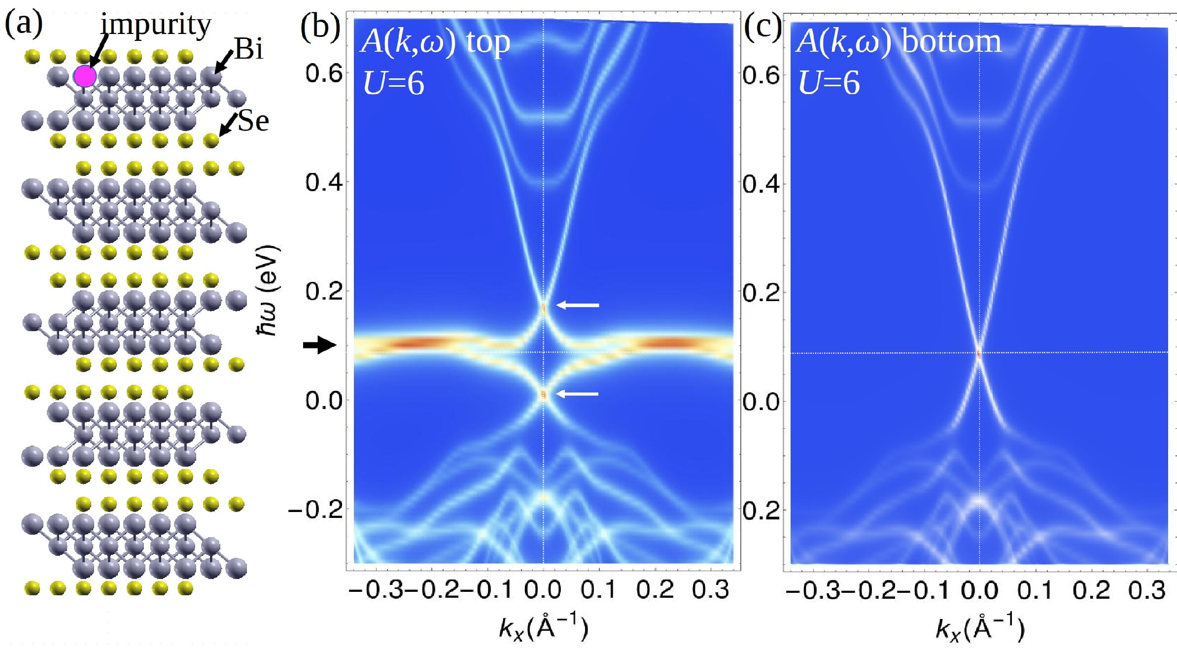
The results of a representative TB calculation with eV are shown in Fig. 1. The supercell structure with a substitutional impurity near the top surface is shown in Fig. 1(a). The spectral function corresponding to atomic layers along the growth direction of the TI slab is calculated by averaging the atom-resolved spectral function over the atoms in a specific layer. The spectral functions of the top and bottom surfaces are shown in Fig. 1(b) and (c), respectively. The presence of surface impurities leads to impurity resonance states that appear as nearly flat bands in the spectral function of the doped surface [Fig. 1(b)], while the undoped surface exhibits unperturbed Dirac states.
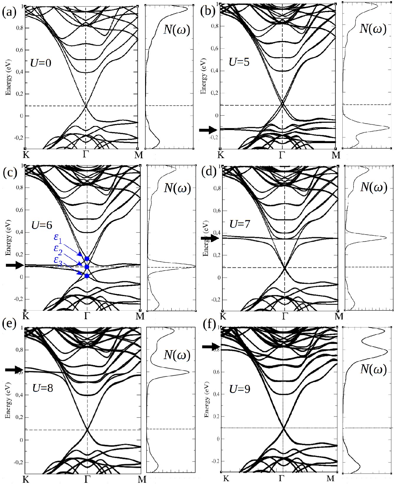
Figure 2 shows the calculated band structures and the density of states (DOS) for a range of impurity potentials . For , the Dirac states of the top and bottom surfaces of the slab are degenerate. With increasing , a nearly dispersionless band emerges in the valence band, and the degeneracy between the top and bottom Dirac states is lifted. The Dirac node of the undoped surface remains pinned at the position of the Dirac node of the pristine system, while the Dirac node of the doped surface is shifted in energy. With increasing the impurity potential further, the impurity band crosses the Dirac node of the top surface and shifts further up in energy. For large , the impurity band merges with the conduction band and the degeneracy of the top and bottom Dirac states is restored.
The impurity states also appear as peaks in the DOS as shown in the right hand-side panels in Fig. 2. Their position is controlled by the non-magnetic impurity potential and coincides with the position of the flat impurity band.
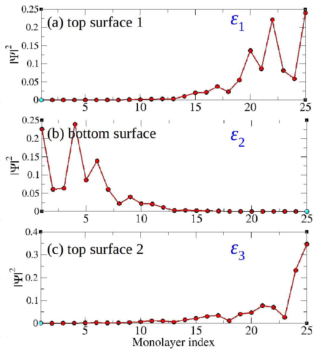
When the impurity resonance state falls in the vicinity of the node, which corresponds to eV in this model [Fig. 2(c)], the Dirac spectrum is drastically modified. The Dirac node of the doped surface is split into two nodes, displaced vertically in energy, and the surface states hybridize with the flat impurity band. Figure 3 shows the spatial distribution of the wavefunctions of the three nodes at , which are marked as in Fig. 2(c) and correspond to the Dirac nodes of the bottom surface and the split nodes of the top surface. The two new nodes at are predominantly localized at the top surface. However, they are not pure surface states and are hybridized with the impurity band localized on the impurity site.
This feature was noticed in previous theoretical work on 3D TIs, which used the scattering matrix approach with and without disorder to study impurity resonances Black-Schaffer et al. (2015); Zhong et al. (2017). In contrast to our tight-binding calculations, this approach does not reply on the use of a supercell. The splitting of the Dirac node due to coherent impurity scattering and the appearance of dispersionless band at zero energy was shown in graphene in the presence of vacancies Zhu et al. (2012). A similar effect was found in ab initio calculations of TI/normal semiconductor heterostructures, where a semiconductor valence band hybridizes with TI surface states Seixas et al. (2015). This result was qualitatively explained by an effective model, based on the low-energy surface state Hamiltonian hybridized with a trivial band from a proximal semiconductor layer. More generally, the possibility of reshaping the topologically protected surface states with localized impurity resonances was demonstrated in Xu et al. (2017) using numerical simulations and scanning tunneling microscopy (STM).
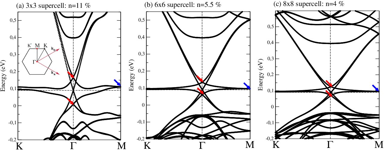
Although the splitting of the Dirac nodes in the presence of disorder was noticed in previous work Black-Schaffer et al. (2015); Zhong et al. (2017), it has not been studied in the context of topology and impurity-controlled nodal structure of DMs. To further illustrate the details of this effect, we show in Fig. 4 the calculated band structures for eV and for different surface impurity concentration. As one can see from Fig. 4(a), the Dirac node of the top surface is split vertically into two nodes (red arrows) and is hybridized with the impurity band, while the bottom surface states remain unaffected by doping. The splitting between the two nodes at decreases with increasing the doping concentration.
An additional doubly degenerate state appears at the Brillouin zone corner ( points) and is marked by a blue arrow in Fig. 4. Here, we consider non-magnetic doping, hence time-reversal symmetry guarantees Kramers degeneracy at the time-reversal invariant momenta and . The surface of Bi2Se3 3D TI is a triangular lattice. Due to the symmetry of the corresponding hexagonal Brillouin zone [see the inset in Fig. 4(a)], there are three non-equivalent points each hosting a doubly degenerate state.
The splitting and generation of new nodes leads to a natural question of whether the topology of the surface states is somehow affected by non-magnetic impurities. As confirmed by the calculations, the nodes remain gapless; however, their number and position change. We verified that the topological properties are preserved in the presence of non-magnetic doping despite the modified nodal structure. The Dirac states in a 3D TI are characterized by spin-momentum locking in the vicinity of the node. We define the helicity as the eigenvalue of the helicity operator , where . This can be visualized as the direction of rotation of the spin of an energy eigenstate as the momentum changes clockwise from to . We found numerically that the helicity of the doped surface, calculated by summing the helicities of the nodes at and , is the same as the helicity of the pristine surface. Thus, the peculiar splitting of the surface state node by impurity resonance necessitates the appearance of new nodes at the Brillouin zone corners to preserve the topology.
III.2 Analytical model of a Dirac spectrum hybridized with an impurity band
We will illustrate the splitting of the Dirac node by hybridization with an impurity band by using an effective low-energy model. We consider the following Hamiltonian
| (1) |
where
| (2) |
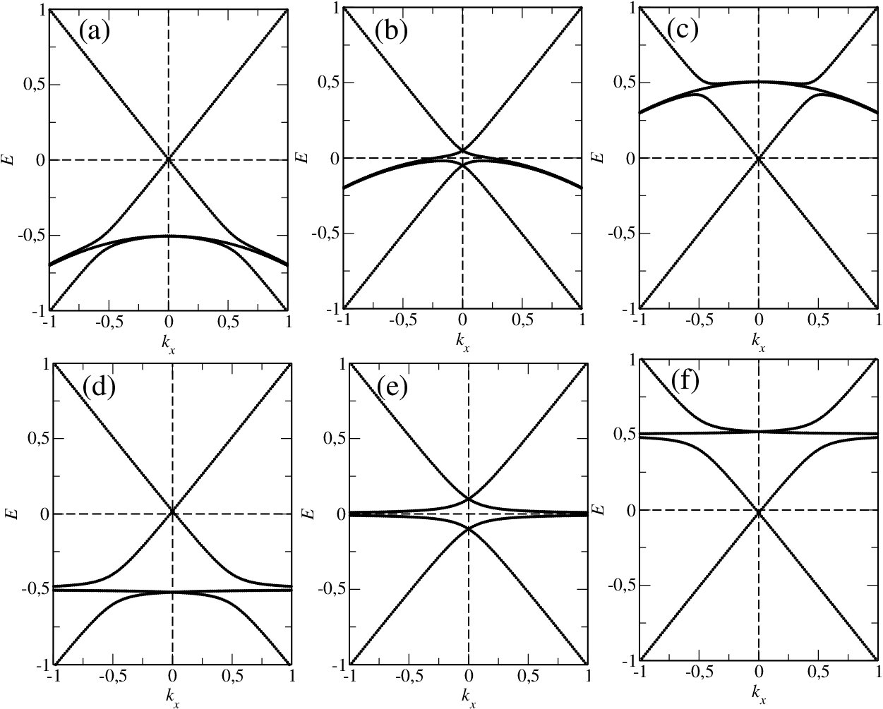
is the Hamiltonian of a 3D TI surface (or graphene); is the Fermi velocity. Here is the coupling matrix, is the coupling strength, is a identity matrix. is the impurity band Hamiltonian, where is the impurity band dispersion. We consider ; the case corresponds to a quadratic band, while gives a flat band. The resulting bandstructures are shown in Fig. 5.
The eigenvalues of the Hamiltonian in Eq. (1) can be found from the following equation
| (3) |
The pair of doubly degenerate states at are given by the solution at
| (4) |
For (), we have and .
III.3 Hybridization via Kondo coupling
For completeness we also analyze the case of correlated impurity bands. While the presence of the flat bands due to impurities is natural, the question can be asked about stability of our results in the presence of correlations. To address this, we now consider an interacting model of a Kondo lattice. We use an analysis based on a localized, -degenerate -band of electrons coupled to a conduction electron band with Dirac cones. The Hamiltonian is
| (5) |
where is an index. which could label different sublattices in a graphene or flux phase Affleck and Marston (1988) structure. The index labels the flavor, and we shall be interested in the limit . The -electrons are presumed to be strongly interacting, satisfying the constraint , where is the fixed filling fraction of the flavor orbitals in each unit cell, which is conserved by . This constraint is enforced by Lagrange multipliers at each site. Invoking the well-established mean field treatment Hewson (1993), the quartic term is decoupled via a Hubbard-Stratonovich transformation with complex local fields , and the Kondo term becomes
| (6) | ||||
Assuming a mean field solution where and are spatially uniform, the mean field Hamiltonian becomes
| (7) | ||||
At this point, we can work in the diagonal basis of , whose eigenvalues are upper and lower bands which touch at certain values where there are Dirac cones. We also define , which is the renormalized -level energy. For simplicity of calculation, we adopt a model of the -electron density of states , with . At , the dimensionless free energy per site per flavor, in units of the -electron half-bandwidth , is
| (8) |
where
| (9) |
is the non-fermionic contribution to the energy,
| (10) |
are the energies of the hybridized - bands (upper and lower), and is defined by , where we position our Fermi level.
The mean field solution is obtained by extremizing with respect to the parameters and . We defer the description of the complete solution to a future publication and describe here some limiting results. Writing , , we obtain a solution to the mean field equations only when . Defining , in the limit where we obtain the equations
| (11) |
where is a solution of the first of these mean field equations. That a critical value of on the order of the bandwidth is necessary in order to obtain a solution is expected from the work of Fradkin and others on magnetic impurities in Dirac systemsWithoff and Fradkin (1990); Cassanello and Fradkin (1996). In the present context, we find then that for , strong interaction physics within a localized -band nominally located below the Fermi level results in a renormalization of the -electron energy, pushing it up to just above the chemical potential, where the -band can effectively hybridize with the Dirac -band and yield the nearly flat bands discussed previously.
IV Discussion and Conclusions
Although it can be problematic to achieve a regular lattice of impurities on a TI surface, there is a strong evidence for impurity-induced states in typical doped TI samples Islam et al. (2018). Moreover, recent ARPES studies suggested that overlapping of impurity resonances with the Dirac node, a situation depicted in Fig. 1(b), could be achieved in the experiment as the binding energy of the node changes with increasing the film thickness Yilmaz et al. (2020). It is also possible to resolve, at least partially, the impurity bands by adjusting the photon energy of the pulse. Another promising platform that can be used to study impurity flat bands are artificially grown impurity superlattices on graphene. Such lattices can be realized by self-assembly of organic molecules on graphene deposited on the substrate Järvinen et al. (2013).
In Fig. 1(b), we considered a situation where material parameters are such that the flat bands occur exactly at the Dirac point of the pristine material. Assuming that the chemical potential is at the Dirac node, this is the most favorable situation which allows access to flat bands. In the new-generation of 3D TIs with composition (Bi,Sb)2B3 (B=Se,Te), chemical potential can be positioned within meV from the Dirac point. The location of the impurity resonances varies greatly with the type of material and dopant Islam et al. (2018). Recent experiments indicate that favourable conditions can be achieved at least for some samples and dopants, e.g. for Cr in Bi2Se3 above the magnetic ordering temperature Yilmaz et al. (2020).
However, in the majority of materials, the above conditions will not be satisfied. Further complications arise from the fact that impurity doping itself may change the position of the Fermi level. For such situations, optical pumping can be used to populate the flat bands. Superconducting or excitonic pairing may occur between carriers residing in the flat bands and will have a transient nature Triola et al. (2017); Pertsova and Balatsky (2018). These ideas can be generalized to pumping of flat, or nearly-flat bands, which do not necessarily originate from impurity-induced states. One fascinating system is a magnetic Weyl semimetal such as the recently discovered Co3Sn2S2, in which the band connecting the Weyl nodes is flattened due to correlations of 3 Co electrons Xu (2020).
In summary, we showed that flat impurity bands arise in impurity-doped Dirac materials. We demonstrate this impurity assisted band structure engineering for a specific case of a three-dimensional topological insulator with non-magnetic impurities on the surface. The impurity flat bands hybridize with the Dirac states and modify their nodal structure. Peculiar features, such as the splitting of the Dirac nodes and generation of additional nodes, are predicted and are explained by a low-energy effective model and topological band theory. We argue that these features are not model specific and are not the artefacts of the supercell approach, and are also present in disordered systems. To test the robustness of these predictions in the presence of electron correlation effects we applied the large- hybridization model to probe the mean field bands and Kondo effect. We find that, while the bands are renormalized, the “extra” Dirac nodes and flat bands persist in interacting model provided the coupling is sufficiently large. These results reinforce our predictions of flat bands engineered via impurity bands and render them experimentally feasible. Predicted impurity-engineered flat bands present a natural platform for exploring interaction-induced phases, beyond the paradigm of twisted bilayer graphene.
Acknowledgements We are grateful to G. Fernando, M. Geilhufe, B. Sinkovic, K. Kaznatcheev, T. Yilmaz and J.X Zhu for useful discussions. Work was supported by the University of Connecticut, the European Unions Seventh Framework Program ERC-2018-SyG HERO-810453, by VILLUM FONDEN via the Centre of Excellence for Dirac Materials (Grant No. 11744) and the Knut and Alice Wallenberg Foundation KAW 2019.0068. Work at Brookhaven National Laboratory was supported by the U.S. Department of Energy, Office of Science, Office of Basic Energy Sciences, under Contract No. DESC0012704.
References
- Wehling et al. (2014) T. Wehling, A. Black-Schaffer, and A. Balatsky, Advances in Physics 63, 1 (2014), eprint https://doi.org/10.1080/00018732.2014.927109, URL https://doi.org/10.1080/00018732.2014.927109.
- Yu et al. (2010) R. Yu, W. Zhang, H.-J. Zhang, S.-C. Zhang, X. Dai, and Z. Fang, Science 329, 61 (2010).
- Chang et al. (2013) C.-Z. Chang, J. Zhang, X. Feng, J. Shen, Z. Zhang, M. Guo, K. Li, Y. Ou, P. Wei, L.-L. Wang, et al., Science 340, 167 (2013), ISSN 0036-8075, eprint https://science.sciencemag.org/content/340/6129/167.full.pdf, URL https://science.sciencemag.org/content/340/6129/167.
- Biswas and Balatsky (2010) R. R. Biswas and A. V. Balatsky, Phys. Rev. B 81, 233405 (2010), URL https://link.aps.org/doi/10.1103/PhysRevB.81.233405.
- Black-Schaffer and Balatsky (2012a) A. M. Black-Schaffer and A. V. Balatsky, Phys. Rev. B 85, 121103 (2012a), URL https://link.aps.org/doi/10.1103/PhysRevB.85.121103.
- Black-Schaffer and Balatsky (2012b) A. M. Black-Schaffer and A. V. Balatsky, Phys. Rev. B 86, 115433 (2012b), URL https://link.aps.org/doi/10.1103/PhysRevB.86.115433.
- Black-Schaffer et al. (2015) A. M. Black-Schaffer, A. V. Balatsky, and J. Fransson, Phys. Rev. B 91, 201411 (2015), URL https://link.aps.org/doi/10.1103/PhysRevB.91.201411.
- Sessi et al. (2016) P. Sessi, R. R. Biswas, T. Bathon, O. Storz, S. Wilfert, A. Barla, K. A. Kokh, O. E. Tereshchenko, K. Fauth, M. Bode, et al., Nat. Commun. 7, 12027 (2016), URL http://dx.doi.org/10.1038/ncomms10559.
- Leykam et al. (2018) D. Leykam, A. Andreanov, and S. Flach, Advances in Physics: X 3, 1473052 (2018), eprint https://doi.org/10.1080/23746149.2018.1473052, URL https://doi.org/10.1080/23746149.2018.1473052.
- Triola et al. (2015) C. Triola, J.-X. Zhu, A. Migliori, and A. V. Balatsky, Phys. Rev. B 92, 045401 (2015), URL https://link.aps.org/doi/10.1103/PhysRevB.92.045401.
- Bistritzer and MacDonald (2011) R. Bistritzer and A. H. MacDonald, Proceedings of the National Academy of Sciences 108, 12233 (2011), ISSN 0027-8424, eprint https://www.pnas.org/content/108/30/12233.full.pdf, URL https://www.pnas.org/content/108/30/12233.
- Cao et al. (2018a) Y. Cao, V. Fatemi, S. Fang, K. Watanabe, T. Taniguchi, E. Kaxiras, and P. Jarillo-Herrero, Nature 556, 80 (2018a), ISSN 1476-4687, URL https://www.nature.com/articles/nature26154#citeas.
- Cao et al. (2018b) Y. Cao, V. Fatemi, S. Fang, K. Watanabe, T. Taniguchi, E. Kaxiras, and P. Jarillo-Herrero, Nature 556, 43 (2018b), ISSN 1476-4687, URL https://doi.org/10.1038/nature26160.
- Kobayashi (2011) K. Kobayashi, Phys. Rev. B 84, 205424 (2011), URL https://link.aps.org/doi/10.1103/PhysRevB.84.205424.
- Pertsova and Canali (2014) A. Pertsova and C. M. Canali, New Journal of Physics 16, 063022 (2014), URL http://stacks.iop.org/1367-2630/16/i=6/a=063022.
- Zhong et al. (2017) M. Zhong, S. Li, H.-J. Duan, L.-B. Hu, M. Yang, and R.-Q. Wang, Scientific Reports 7, 3971 (2017).
- Zhu et al. (2012) W. Zhu, W. Li, Q. W. Shi, X. R. Wang, X. P. Wang, J. L. Yang, and J. G. Hou, Phys. Rev. B 85, 073407 (2012), URL https://link.aps.org/doi/10.1103/PhysRevB.85.073407.
- Seixas et al. (2015) L. Seixas, D. West, A. Fazzio, and S. B. Zhang, Nature Communications 6, 7630 (2015), ISSN 2041-1723, URL https://doi.org/10.1038/ncomms8630.
- Xu et al. (2017) Y. Xu, J. Chiu, L. Miao, H. He, Z. Alpichshev, A. Kapitulnik, R. R. Biswas, and L. A. Wray, Nature Communications 8, 14081 (2017), ISSN 2041-1723, URL https://doi.org/10.1038/ncomms14081.
- Affleck and Marston (1988) I. Affleck and J. B. Marston, Phys. Rev. B 37, 3774 (1988), URL https://link.aps.org/doi/10.1103/PhysRevB.37.3774.
- Hewson (1993) A. C. Hewson, The Kondo Problem to Heavy Fermions, Cambridge Studies in Magnetism (Cambridge University Press, 1993).
- Withoff and Fradkin (1990) D. Withoff and E. Fradkin, Phys. Rev. Lett. 64, 1835 (1990), URL https://link.aps.org/doi/10.1103/PhysRevLett.64.1835.
- Cassanello and Fradkin (1996) C. R. Cassanello and E. Fradkin, Phys. Rev. B 53, 15079 (1996), URL https://link.aps.org/doi/10.1103/PhysRevB.53.15079.
- Islam et al. (2018) M. F. Islam, C. M. Canali, A. Pertsova, A. Balatsky, S. K. Mahatha, C. Carbone, A. Barla, K. A. Kokh, O. E. Tereshchenko, E. Jiménez, et al., Phys. Rev. B 97, 155429 (2018), URL https://link.aps.org/doi/10.1103/PhysRevB.97.155429.
- Yilmaz et al. (2020) T. Yilmaz, A. Pertsova, W. Hines, E. Vescovo, K. Kaznatcheev, A. V. Balatsky, and B. Sinkovic, Journal of Physics: Condensed Matter 32, 145503 (2020), URL https://doi.org/10.1088%2F1361-648x%2Fab6349.
- Järvinen et al. (2013) P. Järvinen, S. K. Hämäläinen, K. Banerjee, P. Häkkinen, M. Ijäs, A. Harju, and P. Liljeroth, Nano Letters 13, 3199 (2013), pMID: 23786613, eprint https://doi.org/10.1021/nl401265f, URL https://doi.org/10.1021/nl401265f.
- Triola et al. (2017) C. Triola, A. Pertsova, R. S. Markiewicz, and A. V. Balatsky, Phys. Rev. B 95, 205410 (2017), URL https://link.aps.org/doi/10.1103/PhysRevB.95.205410.
- Pertsova and Balatsky (2018) A. Pertsova and A. V. Balatsky, Phys. Rev. B 97, 075109 (2018), URL https://link.aps.org/doi/10.1103/PhysRevB.97.075109.
- Xu (2020) Y. Xu, Nat. Comm. 11, 3985 (2020), URL https://www.nature.com/articles/s41467-020-17234-0.