Eternally non-Markovian dynamics of a qubit interacting with a single-photon wavepacket

Abstract

An evolution of a two-level system (qubit) interacting with a single-photon wave packet is analyzed. It is shown that a hierarchy of master equations gives rise to phase covariant qubit evolution. The temporal correlations in the input field induce nontrivial memory effects for the evolution of a qubit. It is shown that in the resonant case whenever time-local generator is regular (does not display singularities) the qubit evolution never displays information backflow. However, in general the generator might be highly singular leading to intricate non-Markovian effects. A detailed analysis of the exponential profile is provided which allows to illustrate all characteristic feature of the qubit evolution.

I Introduction

Any real quantum system is never perfectly isolated and hence has to be treated as an open system BP02 . Therefore, its evolution is no longer unitary and gives rise to well known processes of dissipation, decay, and decoherence induced by the nontrivial system–environment interaction Alicki . When the interaction between system and environment is sufficiently weak and the characteristic time scales are well separated one uses well known Markovian approximation governed by the celebrated Markovian master equation $\dot{\rho}=\mathcal{L}\rho$, with $\mathcal{L}$ being the Gorini-Kossakowski-Lindblad-Sudarshan (GKLS) generator GKS ; L

$$\mathcal{L}(\rho)=-i[H_{S},\rho]+\sum_{k}\gamma_{k}\Big{(}L_{k}\rho L_{k}^{\dagger}-\frac{1}{2}\{L_{k}^{\dagger}L_{k},\rho\}\Big{)},$$ (1)

where $H_{S}$ stands for the effective system’s Hamiltonian (including Lamb shift correction), $L_{k}$ are jump (Lindblad) operators, and $\gamma_{k}\geq 0$ (in what follows we keep $\hbar=1$). In non-Markovian regime due to correlations between the system and environment the reduced evolution of the system is no longer governed by (1). One observes characteristic memory effects such as information bacflow or recoherence. Laboratory techniques of quantum engineering enable nowadays to test experimentally theoretical descriptions and concepts of non-Markovian quantum dynamics. Scope of applications of these theoretical tools is constantly growing and the field of non-Markovian quantum processes attracts a lot of interest (cf. recent reviews NM1 ; NM2 ; NM3 ; NM4 together with Piilo1 ; Piilo2 ; Modi2 ; Modi3 and the recent tutorial Modi4 ).

In this paper we study non-Markovian dynamics of the two-level system (qubit) interacting with a single-photon wave packet and the vacuum field. So we consider a scattering of a single-photon field on the two-level system. Propagating wave packets of light of definite numbers of photons play a key role in photonics. The continuous-mode single-photon state L00 ; M08 is an example of non-classical states of light having applications in quantum computation KLM01 ; Ralph03 , metrology D08 ; Munro02 , communication Scarani09 , and simulation Aaronon11 . Constantly developing techniques of producing, storing and detecting of single-photon states of light can serve in a wide range of practical applications CWSS13 ; PSZ13 ; RR15 ; Leong2016 ; Zoller2017 .

We describe the evolution of qubit which is driven by the single-photon field and at the same time it undergoes damping process. Note that the single-photon field not only drives the system but it is also the source of stimulated emission. The key ingredient of our model are temporal correlations present in the input state of the field which is characterised by the time dependent profile $\xi(t)$ (for $t\geq 0$). The temporal correlations are responsible for all non-Markovian memory effects of the qubit dynamics. The reduced evolution of the qubit, obtained within the input-output formalism GarCol85 , is represented then by a hierarchy of coupled equations GEPZ98 ; WMSS11 ; BCBC12 ; Gough12a ; Baragiola17 ; DSC17 ; DSC19 ; D20 . We provide the analytical solution to this hierarchy of equations for any initial state of the system and an arbitrary profile $\xi(t)$ and use it to show that the set of these equations is equivalent to a single time-local master equation. The price one pays for this reduction is highly nontrivial structure of time-dependent rates in the time-local master equation. The corresponding time-local generator is phase covariant and its general properties, recently studied, providing us with the necessary tools to analyze non-Markovanity effects SKHD16 ; Sabrina-2016 ; Sabrina-NJP ; Francesco ; HSH19 ; Sergey-2020 . The time dependent rates governing damping (cooling), heating and decoherence processes are fully characterized by the wave packet profile. Such formulae were never presented before. An immediate consequence of our analysis is the observation that in general the dynamical map governing the qubit evolution is not invertible which implies the singularity of rates in the corresponding time-local master equation. Similar observation for phase covariant dynamics was recently reported in Francesco . Non-invertible maps were considered in quantum optics scenario, for instance, in Cresser1 ; Cresser2 ; Hou ; SKHD16 (cf. also PRL-2018 ; CC19 and recent paper Jyrki-2021 ).

The analyzed system provides excellent platform to test indicators of non-Markovianity. It turns out that in the resonant case, which is of particular importance in photonic experiments, the evolution is never CP-divisible but it also never displays information backflow. We provide a detailed analysis of the qubit evolution interacting with exponential profile. In this case we are able to derive both analytical formulae for time-local rates and characterize the regime when the dynamics does not allow for information backflow.

The paper is organized as follows. Section II introduces basic properties of dynamical maps and discusses recent concepts of Markovianity. In Section III we introduce the hierarchy equations describing the reduced evolution of the two-level system interacting with the single-photon field and the vacuum, and eventually provide the solution for the qubit evolution. Sections IV and V contain the general properties of qubit evolution and the corresponding time-local generator, respectively. In Section VI the detailed analysis of the exponential profile is carried out: we discuss both the resonant and off resonant case. The key observation is that for an exponential profile the qubit evolution is eternally non-Markovian Erika , that is, the corresponding time-local generator always contains a strictly negative transition rate for any time $t>0$. Actually, we conjecture that this characteristic feature holds for an arbitrary photon profile. Final conclusions are presented in section VII. Technical details are presented in the appendices.

II Preliminaries

Evolution of a quantum system is represented by a dynamical map $\{\Lambda_{t}\}_{t\geq 0}$ which maps an initial state $\rho$ at $t=0$ into a state at a current time $t$, i.e. $\rho(t)=\Lambda_{t}(\rho)$. Usually, the map is realized as a reduced evolution of the system + environment

$$\rho(t)=\mathrm{Tr}_{E}\left(U(t)\rho\otimes\rho_{E}U^{\dagger}(t)\right),$$ (2)

where $U(t)$ is the unitary evolution operator corresponding to the total Hamiltonian $H=H_{S}+H_{E}+H_{int}$, and ${\rm Tr}_{E}$ denotes the partial trace over the environmental degrees of freedom BP02 . As a result (2) gives rise to a map $\rho\to\rho(t)$ which is completely positive and trace preserving (CPTP). Recall that any such map allows for the Kraus representation

$$\Lambda_{t}(\rho)=\sum_{\alpha}K_{\alpha}(t)\rho K_{\alpha}^{\dagger}(t),$$ (3)

where the time-dependent Kraus operator $K_{\alpha}(t)$ satisfies the additional normalization condition $\,\sum_{\alpha}K_{\alpha}^{\dagger}(t)K_{\alpha}(t)=\mathbbm{1}\,$ which guaranties that the map $\Lambda_{t}$ is trace-preserving, i.e. ${\rm Tr}\,\Lambda_{t}(\rho)={\rm Tr}\,\rho$ for any $\rho$. Reduced dynamics defined via (2) provides a generalization of Markovian dynamical semigroups governed by GKLS generator (1). For differentiable quantum dynamical map the system’s density operator $\rho(t)$ satisfies time-local master equation

$$\dot{\rho}(t)=\mathcal{L}_{t}\rho(t),$$ (4)

with time-dependent generator $\mathcal{L}_{t}$. Note, that given $\{\Lambda_{t}\}_{t\geq 0}$ the time-local generator is formally defined by $\,\mathcal{L}_{t}=\dot{\Lambda}_{t}\Lambda_{t}^{-1}$ provided the map $\Lambda_{t}$ is invertible. If the map is not invertible at $t=\tau$, then $\mathcal{L}_{t}$ displays singularities at $\tau$. This is not only a mathematical curiosity. Non-invertible maps were already considered in quantum optical systems Francesco ; Cresser1 ; Cresser2 ; Hou ; SKHD16 (cf. also PRL-2018 ; CC19 and recent papers Piilo1 ; Piilo2 ). The system we study in this paper gives rise to a perfectly regular map $\{\Lambda_{t}\}_{t\geq 0}$ which, however, needs not be invertible and hence the corresponding master equation is governed by a singular generator. Interestingly, singularities of $\mathcal{L}_{t}$ provide important physical insight into the dynamical properties of the system.

Any time-local generator $\mathcal{L}_{t}$ has essentially the same structure as (1), where now the effective Hamiltonian $H_{S}$, the noise operators $L_{k}$, and the transition rates $\gamma_{k}$ are time-dependent. Given $\mathcal{L}_{t}$ the formal solution for the dynamical map reads as follows

$$\Lambda_{t}=\mathcal{T}\exp\left(\int_{0}^{t}\mathcal{L}_{\tau}d\tau\right),$$ (5)

where $\mathcal{T}$ stands for the chronological product. It should be stressed that in the time-dependent case transition rates $\gamma_{k}(t)$ are not necessarily non-negative. This makes the characterization of admissible generators extremely hard Erika ; Angel . Actually, temporal negativity of $\gamma_{k}(t)$ is usually interpreted as manifestation of non-Markovianity. A quantum dynamical map $\{\Lambda_{t}\}_{t\geq 0}$ is called divisible if for any $t\geq s$ one has $\,\Lambda_{t}=V_{t,s}\Lambda_{s}$. Note, that any invertible map is necessarily divisible since $V_{t,s}=\Lambda_{t}\Lambda_{s}^{-1}$. However, for not invertible maps the issue of divisibility is much more subtle BOGNA ; datta ; Acin-cor ; Johansson ; PRL-2018 ; CC19 ; Jyrki-2021 . In a recent paper Ujan the construction of propagators for non-invertible maps in terms of generalized inverse was proposed. One calls the map $\{\Lambda_{t}\}_{t\geq 0}$ P-divisible if $V_{t,s}$ is positive and trace-preserving, and CP-divisible if $V_{t,s}$ is completely positive and trace-preserving. Following RHP we call the evolution represented by $\{\Lambda_{t}\}_{t\geq 0}$ Markovian if it is CP-divisible. An invertible map is CP-divisible if and only if all rates satisfy $\gamma_{k}(t)\geq 0$. This is a direct generalization of Markovian semigroup. For non-invertible maps the full characterization is still missing PRL-2018 . One of the most interesting implication of non-Markovianity is an information backflow defined as follows BLP : if the evolution is Markovian, then for any pair of initial states $\rho_{1}$ and $\rho_{2}$

$$\frac{d}{dt}\|\Lambda_{t}(\rho_{1}-\rho_{2})\|_{1}\leq 0,$$ (6)

where $\|X\|_{1}={\rm Tr}|X|$ denotes the trace norm of $X$. Note, that the quantity $\|\rho_{1}-\rho_{2}\|_{1}$ describes the distinguishability of $\rho_{1}$ and $\rho_{2}$. Now, the violation of (6) is interpreted as an information backflow (from the environment to the system). In what follows we call (6) a BLP condition. An interesting example of the qubit evolution which satisfies BLP condition but is not CP-divisible was provided in Erika : the corresponding time-local generator reads as follows

$$\mathcal{L}_{t}(\rho)=\frac{1}{2}\sum_{k=1}^{3}\gamma_{k}(t)(\sigma_{k}\rho\sigma_{k}-\rho),$$ (7)

with $\gamma_{1}=\gamma_{2}=1$ and $\gamma_{3}(t)=-\tanh t<0$. Interestingly, one of the rate is always negative (for $t>0$) but still the corresponding dynamical map is completely positive. The authors of Erika call such evolution eternally non-Markovian. This analysis was further generalized in Nina and Kasia for qudit systems. In this paper we face another example of qubit evolution for which for any $t>0$ some rate $\gamma_{k}(t)$ is negative. Nevertheless, the evolution is represented by completely positive dynamical map. This might be, therefore, considered as an another example of eternally non-Markovian evolution. This example, however, corresponds to well motivated physical system representing a qubit interacting with an incoming external photon.

It should be stressed that dealing with evolution of open quantum systems the very notion of Markovian evolution is often used in different contexts and actually several concept of (non)Markovian evolution are available in the current literature (cf. recent reviews NM1 ; NM2 ; NM3 ; NM4 and Piilo1 ; Piilo2 ). Authors of NM4 shown an intricate hierarchy of various notions of quantum Markovianity and clearly indicates that this concept is highly context-dependent. In the present paper we are characterizing non-Markovian process using only the properties of the corresponding dynamical map. An interesting approach to quantum non-Markovianity beyond a dynamical map based on so called quantum process tensor was recently analyzed in Modi2 ; Modi3 (cf. also recent tutorial Modi4 ). This approach was further applied in Andrea1 ; Andrea2 ; Filippov-Modi in the study of open quantum systems dynamics.

A simple indicator of non-Markovianity was proposed in LPP13 (see also further discussion in CMM17 ): for any Markovian evolution

$$\frac{d}{dt}|{\rm det}\Lambda_{t}|\,\leq\,0.$$ (8)

The volume of the accessible states at time $t$ is given by $\mathrm{Vol}(t)=|{\rm det}\Lambda_{t}|\rm{Vol}(0)$ and hence (8) implies monotonic decrees of $\rm{Vol}(t)$. Any P-divisible (and hence also CP-divisible) satisfies (8). In what follows we analyze a qubit interacting with an incoming photon field and show how the photon’s profile $\xi(t)$ decides about the validity of BLP condition (6), geometric condition (8), and eventually (non)Markovianity of the evolution.

III Hierarchy of master equations

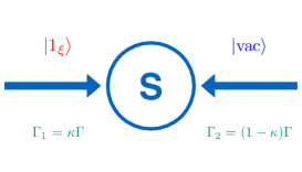
Figure 1: The system S interacts from the left with a single-photon field $|1_{\xi}\rangle$ and from the right with a vacuum field $|vac\rangle$. We introduced $\Gamma=\Gamma_{1}+\Gamma_{2}$ and the parameter $\kappa\in[0,1]$ such that $\Gamma_{1}=\kappa\Gamma$, and $\Gamma_{2}=(1-\kappa)\Gamma$.

We consider a two-level system interacting by two channels with a continuous-mode electromagnetic field L00 schematically depicted in Fig. 1. The system interacts with the single-photon field incoming from the left and the vacuum field incoming from the right. We assume that, in general, the coupling of the system with the single-photon field and the vacuum could be different. In the model some standard assumptions in quantum optics are made (rotating wave-approximation, a flat coupling constant, and an extension of the lower limit of integration over frequency to minus infinity). The bandwidth of the spectrum is assumed to be much smaller that the central frequency of the pulse $\Delta\omega\ll\omega_{c}$ and the central frequency $\omega_{c}$ is taken to be close the transition frequency of the two-level system $\omega_{0}$. A detailed discussion on the assumptions for the model one can find, for instance, in FTVRS17 . We assume that the composed system is initially in the state $\rho(0)\otimes|1_{\xi}\rangle\langle 1_{\xi}|\otimes|vac\rangle\langle vac|$, where

$$|1_{\xi}\rangle=\int_{-\infty}^{+\infty}d\omega\hat{\xi}(\omega)a^{\dagger}_{1}(\omega)|vac\rangle$$ (9)

and $|vac\rangle$ is the continuous-mode vacuum state, $a^{\dagger}_{i}(\omega)$, $a_{i}(\omega)$ $(i=1,2)$ are annihilation and creation operators of $\omega$-mode satisfying the standard canonical commutation relations

$$[a_{i}(\omega),a^{\dagger}_{j}(\omega^{\prime})]=\delta_{ij}\delta(\omega-\omega^{\prime}).$$ (10)

The profile of the photon in the time domain is defined as follows

$$\xi(t)=\int_{-\infty}^{+\infty}d\omega\hat{\xi}(\omega)e^{-i(\omega-\omega_{c})t}$$ (11)

with the normalization condition

$$\int_{0}^{+\infty}dt|\xi(t)|^{2}=\int_{-\infty}^{+\infty}d\omega|\hat{\xi}(\omega)|^{2}=1.$$ (12)

Note that the profile, $\xi(t)$, defines a slow varying envelope of the time amplitude of the pulse. Since we are close to the resonance $(\omega_{c}\approx\omega_{0}$) it is convenient to pass to the interaction picture defined by the central frequency $\omega_{c}$, that is, a qubit state $\rho(t)$ ‘rotates’ via $e^{-i\omega_{c}\sigma_{z}/2}$. The interaction Hamiltonian in the interaction-picture has the form

$$H_{int}(t)=i\sqrt{\Gamma_{1}}\left(\sigma_{-}a^{\dagger}_{1}(t)-\sigma_{+}a_{1}(t)\right)+i\sqrt{\Gamma_{2}}\left(\sigma_{-}a_{2}^{\dagger}(t)-\sigma_{+}a_{2}(t)\right),$$ (13)

where $a_{i}(t)$ and $a^{\dagger}_{i}(t)$ are quantum white-noise operators GZ10 obeying the communication relation

$$[a_{i}(t),a_{j}^{\dagger}(t^{\prime})]=\delta_{ij}\delta(t-t^{\prime}).$$ (14)

Using the ‘rotating frame’ one derives the following hierarchy of coupled equations for the family of qubit operators ${\varrho}^{kl}$ with $k,l=0,1$

$$\dot{\varrho}^{11}(t)=\mathcal{L}{\varrho}^{11}(t)+\sqrt{\Gamma_{1}}\;\xi^{\ast}(t)[\sigma_{-},{\varrho}^{10}(t)]-\sqrt{\Gamma_{1}}\;\xi(t)[\sigma_{+},{\varrho}^{01}(t)],$$ (15)

$$\dot{{\varrho}}^{10}(t)=\mathcal{L}{\varrho}^{10}(t)-\sqrt{\Gamma_{1}}\;\xi(t)\left[\sigma_{+},{\varrho}^{00}(t)\right],$$ (16)

$$\dot{{\varrho}}^{01}(t)=\mathcal{L}{\varrho}^{01}(t)+\sqrt{\Gamma_{1}}\;\xi^{\ast}(t)\left[\sigma_{-},{\varrho}^{00}(t)\right],$$ (17)

$$\dot{{\varrho}}^{00}(t)=\mathcal{L}{\varrho}^{00}(t)$$ (18)

with the super-operator

$$\mathcal{L}({\varrho})=-\frac{i\Delta_{0}}{2}[{\varrho},\sigma_{z}]-\frac{\Gamma}{2}\left\{\sigma_{+}\sigma_{-},{\varrho}\right\}+\Gamma\sigma_{-}{\varrho}\sigma_{+},$$ (19)

where $\Delta_{0}=\omega_{c}-\omega_{0}$, $\sigma_{z}=|e\rangle\langle e|-|g\rangle\langle g|$, $\Gamma=\Gamma_{1}+\Gamma_{2}$, and $\Gamma_{1},\Gamma_{2}\geq 0$. By $|e\rangle$ and $|g\rangle$ the excited and ground states of the two-level system are respectively denoted. One defines the density operator of the system $\rho(t):=\varrho^{11}(t)$, and initially

$$\varrho^{11}(0)=\varrho^{00}(0)=\rho(0)\ ,\ \ \varrho^{01}(0)=\varrho^{10}(0)=0.$$ (20)

Note, that $\varrho^{10}(t)=\left(\varrho^{01}(t)\right)^{\dagger}$. The system is initially in an arbitrary state, $\rho(0)$. The set of equations defines the qubit dynamics during the scattering process. The derivations of the set of equations describing the evolution of a quantum system interacting with the single-photon field was given, for instance, in GEPZ98 ; BCBC12 ; WMSS11 ; Gough12a ; Baragiola17 . The details of its determination in a collision model Ciccarello2021 one can find in DSC17 . Let us notice that the above set of equations can be written in the form

$$\frac{d}{dt}\begin{pmatrix}\varrho^{11}(t)\\ \varrho^{10}(t)\\ \varrho^{01}(t)\\ \varrho^{00}(t)\end{pmatrix}=\begin{pmatrix}\mathcal{L}&\mathcal{L}_{\xi}&\mathcal{L}_{\xi}^{\ddagger}&0\\ 0&\mathcal{L}&0&\mathcal{L}_{\xi}^{\ddagger}\\ 0&0&\mathcal{L}&\mathcal{L}_{\xi}\\ 0&0&0&\mathcal{L}\end{pmatrix}\begin{pmatrix}\varrho^{11}(t)\\ \varrho^{10}(t)\\ \varrho^{01}(t)\\ \varrho^{00}(t)\end{pmatrix},$$ (21)

where we introduced

$$\mathcal{L}_{\xi}(X)=\sqrt{\Gamma_{1}}\;\xi^{*}(t)[\sigma_{-},X],$$ (22)

and its dual

$$\mathcal{L}^{\ddagger}_{\xi}(X)=-\sqrt{\Gamma_{1}}\;\xi(t)[\sigma_{+},X],$$ (23)

where ${\rm Tr}(\mathcal{L}^{\ddagger}_{\xi}(X)Y)={\rm Tr}(X\mathcal{L}_{\xi}(Y))$ for any pair $X,Y$.

Note, that operators $\varrho^{01}(t)$ and $\varrho^{10}(t)$ are not Hermitian. However, introducing a pair of Hermitian operators

$$\varrho^{2}(t):=\varrho^{01}(t)+\varrho^{10}(t)\ ,\ \ \ \varrho^{3}(t):=-i(\varrho^{01}(t)-\varrho^{10}(t))\ ,$$ (24)

together with $\varrho^{1}(t):=\varrho^{11}(t)$ and $\varrho^{4}(t):=\varrho^{00}(t)$, the systems of equations (21) may be rewritten as follows

$$\dot{\varrho}^{1}(t) = \mathcal{L}\varrho^{1}(t)-\frac{i}{2}\sqrt{\Gamma_{1}}\,\Big{(}[\sigma^{\xi}_{y},\varrho^{2}(t)]+[\sigma^{\xi}_{x},\varrho^{3}(t)]\Big{)},$$

$$\dot{\varrho}^{2}(t) = \mathcal{L}\varrho^{2}(t)-i\sqrt{\Gamma_{1}}\,[\sigma^{\xi}_{y},\varrho^{4}(t)],$$

$$\dot{\varrho}^{3}(t) = \mathcal{L}\varrho^{3}(t)-i\sqrt{\Gamma_{1}}\,[\sigma^{\xi}_{x},\varrho^{4}(t)],$$ (25)

$$\dot{\varrho}^{4}(t) = \mathcal{L}\varrho^{4}(t),$$

where

$$\sigma^{\xi}_{x}:=\xi^{*}\sigma_{-}+\xi\sigma_{+}=\left(\begin{array}[]{cc}0&\xi^{*}\\ \xi&0\end{array}\right),\ \ \ \ \sigma^{\xi}_{y}:=i(\xi^{*}\sigma_{-}-\xi\sigma_{+})=\left(\begin{array}[]{cc}0&i\xi^{*}\\ -i\xi&0\end{array}\right).$$ (26)

The set of equations (III) has a structure of hierarchical master equations of motion (HEOM) Florian ; Tanimura

$$\dot{\varrho}^{i}(t)=\sum_{j=1}^{n}\mathcal{L}_{ij}\varrho^{j}(t)\ ,\ \ i,j=1,\ldots,n,$$ (27)

for some $n\geq 1$. In Eq. (27) only $\varrho^{1}$ is considered as a system’s state and the remaining operators $\varrho^{i}$ are auxiliary objects. For the system (III) one has $n=2^{2}$. Interestingly, in a more general case, when the field is prepared in $N$-photon state, the evolution of the system is governed by the set of $(N+1)^{2}$ coupled equations BCBC12 ; DSC19 .

Note, that if $\xi(t)=0$, i.e. there is no photon, then (III) reduces to

$$\dot{\varrho}^{k}(t)=\mathcal{L}\varrho^{k}(t)\ ,\ \ \ k=1,2,3,4,$$ (28)

and the auxiliary operators $\{\varrho^{2},\varrho^{3},\varrho^{4}\}$ are totally decoupled from the evolution of the system itself. The photon profile $\xi(t)$ makes the systems (III) nontrivial and eventually influences the evolution of $\rho(t):=\varrho^{1}(t)$. As we shall see such evolution is no longer Markovian.

IV General properties of the qubit dynamics

The hierarchy of equations (21) may be solved (cf. Appendix A) and eventually one finds the following dynamical map $\Lambda_{t}$ representing qubit evolution D20

$$\rho(0)\ \to\ {\rho}(t)=\Lambda_{t}\rho(0)=\left(\begin{array}[]{cc}1-P_{e}(t)&C(t)\rho_{ge}(0)\\ C^{\ast}(t)\rho_{eg}(0)&P_{e}(t)\\ \end{array}\right),$$ (29)

where the population of the excited state $P_{e}(t)=\rho_{ee}(t)$ reads as follows

$$P_{e}(t)=A(t)+B(t)P_{e}(0),$$ (30)

together with

$$A(t)=\kappa\Gamma e^{-\Gamma t}\left|\int_{0}^{t}ds\xi(s)e^{\left(-i\Delta_{0}+\frac{\Gamma}{2}\right)s}\right|^{2},$$ (31)

$$B(t)=e^{-\Gamma t}\left(1-4\kappa\Gamma\mathrm{Re}\int_{0}^{t}ds\xi^{\ast}(s)e^{\left(i\Delta_{0}+\frac{\Gamma}{2}\right)s}\int_{0}^{s}d\tau\xi(\tau)e^{\left(-i\Delta_{0}-\frac{\Gamma}{2}\right)\tau}\right),$$ (32)

and

$$C(t)=e^{\left(-i\Delta_{0}-\frac{\Gamma}{2}\right)t}\left(1-2\kappa\Gamma\int_{0}^{t}ds\xi^{\ast}(s)e^{\left(i\Delta_{0}-\frac{\Gamma}{2}\right)s}\int_{0}^{s}d\tau\xi(\tau)e^{\left(-i\Delta_{0}+\frac{\Gamma}{2}\right)\tau}\right).$$ (33)

We introduce here the parameter $\kappa=\Gamma_{1}/\Gamma$, hence $\kappa\in[0,1]$. Thus, if $\kappa=0$, we deal with the system interacting only with the vacuum part, and if $\kappa=1$, we observe only an interaction with the single-photon field. The above formulae provide a complete description of the qubit evolution for an arbitrary photon profile $\xi(t)$. Note, that $B(t)$ together with $\{C(t),C^{*}(t)\}$ define time dependent eigenvalues of the dynamical map $\Lambda_{t}$:

$$\Lambda_{t}(|e\rangle\langle e|-|g\rangle\langle g|)=B(t)(|e\rangle\langle e|-|g\rangle\langle g|)\ ,\ \ \Lambda_{t}|g\rangle\langle e|=C(t)|g\rangle\langle e|\ ,\ \ \Lambda_{t}|e\rangle\langle g|=C^{*}(t)|e\rangle\langle g|.$$ (34)

Clearly, the evolution highly depends upon the photon profile and the dependence of $\{A(t),B(t),C(t)\}$ upon $\xi(t)$ is quite nontrivial. However, the asymptotic state is universal: the atom eventually relaxes to the ground state $|g\rangle$ irrespective of $\xi(t)$. It follows from the asymptotic analysis

$$\lim_{t\to+\infty}A(t)=0,\;\;\lim_{t\to+\infty}B(t)=0,\;\;\lim_{t\to+\infty}C(t)=0.$$ (35)

Hence, we obtain $\displaystyle{\lim_{t\to+\infty}}P_{e}(t)=0$ and $\displaystyle{\lim_{t\to+\infty}}\rho(t)=|g\rangle\langle g|$. It should be stressed, however, that $|g\rangle\langle g|$ is not an invariant state of the evolution. This is essential difference between Markovian semigroup and non-Markovian evolution PRA-Saverio . For a semigroup an asymptotic state always defines an invariant state. However, for the evolution (29) if one starts with $\rho(0)=|g\rangle\langle g|$, then

$$\rho(t)=A(t)|e\rangle\langle e|+[1-A(t)]|g\rangle\langle g|,$$ (36)

that is, the evolution does not create coherence but it does create population controlled by $A(t)$ which asymptotically vanishes. The problem of an optimal profile, i.e. a profile maximizing $A(t)=P_{e}(t)$ for some finite $t$, was analyzed by several authors SAL10a ; Rephali2010 ; WMSS11 ; RB17 . Our analysis allows to formulate the following

Proposition 1

If $\rho(0)=|g\rangle\langle g|$, then the maximal population of the excited state $P_{e}(t)$ at time $t>0$ reads as follows

$$P^{\rm max}_{e}(t):=\max_{\xi(t)}P_{e}(t)=\kappa\left(1-e^{-\Gamma t}\right),$$ (37)

and is realized only at the resonance (i.e. $\Delta_{0}=0$) by the following pulse

$$\xi(\tau)=\sqrt{\frac{\Gamma}{e^{\Gamma t}-1}}\,e^{\frac{\Gamma}{2}\tau}$$ (38)

for $\tau\in[0,t]$, and $\xi(\tau)=0$ for $\tau>t$.

For the proof cf. Appendix B. Let us note that for any given profile, $\xi(t)$, one may discuss the problem of choosing its parameters which provides the maximal temporal excitation of the system WMSS11 ; RB17 .

We conclude this section with the following statements. There are two essentially different scenario for the qubit evolution:

1. The quantities $B(t)>0$ and $|C(t)|>0$ for all $t\geq 0$. In this case the dynamical map $\Lambda_{t}$ is invertible (eigenvalues $\{B(t),C(t),C^{*}(t)\}$ do not vanish), that is, knowing a qubit state $\rho(t)$ at time $t$ one may reconstruct the initial state $\rho(0)$.

2. The dynamical map $\Lambda_{t}$ is no longer invertible, i.e. there exists $t<\infty$ such that either $B(t)=0$ or $C(t)=0$. Note, that whenever $B(t)=0$, the density operator $\rho(t)$ reads as

   $${\rho}(t)=\left(\begin{array}[]{cc}1-A(t)&C(t)\rho_{ge}(0)\\ C^{\ast}(t)\rho_{eg}(0)&A(t)\\ \end{array}\right),$$ (39)

   and hence it does not depend upon initial population $P_{e}(0)$. Actually, diagonal elements display the same structure as in (36). So if initially $\rho_{ge}(0)=(\rho_{eg}(0))^{\dagger}=0$, then all trajectories of different $P_{e}(0)$ cross at some point. Whenever $C(t)=0$, then

   $${\rho}(t)=\left(\begin{array}[]{cc}1-P_{e}(t)&0\\ 0&P_{e}(t)\\ \end{array}\right),$$ (40)

   and for this moment the information about qubit coherence is lost.

V Time-local generator and non-Markovianity conditions

To discuss non-Markovianity of qubit evolution it is convenient to introduce the corresponding time-local master equation for the density matrix. The formula (29) for time evolution of the qubit density operator $\rho(t)$ defines a dynamical map $\rho(0)\to\Lambda_{t}\rho(0)$. By differentiating (29) with respect to time, one easily finds that $\Lambda_{t}$ satisfies time-local master equation $\dot{\Lambda}_{t}=\mathcal{L}_{t}\Lambda_{t}$, with the following time-local generator

$$\mathcal{L}_{t}(\rho)=-i\frac{\omega(t)}{2}[\sigma_{z},\rho]+\frac{\gamma_{+}(t)}{2}\left(\sigma_{+}\rho\sigma_{-}-\frac{1}{2}\{\sigma_{-}\sigma_{+},\rho\}\right)+\frac{\gamma_{-}(t)}{2}\left(\sigma_{-}\rho\sigma_{+}-\frac{1}{2}\{\sigma_{+}\sigma_{-},\rho\}\right)+\frac{\gamma_{z}(t)}{2}(\sigma_{z}\rho\sigma_{z}-\rho),$$ (41)

where $\sigma_{\pm}=\frac{1}{2}(\sigma_{x}\pm i\sigma_{y})$, and $\sigma_{x}$, $\sigma_{y}$, $\sigma_{z}$ are the Pauli operators. The real valued time-dependent rates $\gamma_{+}(t)$, $\gamma_{-}(t)$, and $\gamma_{z}(t)$, describing, respectively, pumping, damping and pure dephasing, are defined as follows

$$\gamma_{+}(t)=2\frac{\dot{A}(t)B(t)-A(t)\dot{B}(t)}{B(t)}\ ,\ \ \ \gamma_{-}(t)=-2\frac{\dot{B}(t)}{B(t)}-\gamma_{+}(t),$$ (42)

$$\gamma_{z}(t)=\frac{1}{2}\frac{\dot{B}(t)}{B(t)}-\frac{\frac{d}{dt}{|C(t)|}}{|C(t)|}=\frac{1}{2}\frac{\dot{B}(t)}{B(t)}-{\rm Re}\,\frac{\dot{C}(t)}{C(t)},$$ (43)

and

$$\omega(t)=\frac{\dot{C}(t)|C(t)|-C(t)\frac{d}{dt}|C(t)|}{iC(t)|C(t)|}={\rm Im}\,\frac{\dot{C}(t)}{C(t)}.$$ (44)

It should be emphasized that time-local generator $\mathcal{L}_{t}$ becomes singular whenever $B(t)=0$ or $C(t)=0$. In this case $\gamma_{\pm}(t)$ and $\gamma(t)$ diverge. Nevertheless, the dynamical map $\Lambda_{t}=\mathcal{T}\exp(\int_{0}^{t}\mathcal{L}_{u}du)$ is always well defined for any $t\geq 0$. It shows that perfectly regular hierarchy of the equations (15)-(16) may give rise to singular master equation for a system’s density operator $\rho(t)$. One can easily check that if $\xi(t)=0$ for any $t\geq 0$, then we get $A(t)=0,\,B(t)=e^{-\Gamma t},\,C(t)=e^{-\left(i\Delta_{0}+\Gamma/2\right)t}$, and $\gamma_{+}(t)=0,\,\gamma_{-}(t)=2\Gamma,\,\gamma_{z}(t)=0,\,\omega(t)=\Delta_{0}$, that is, $\mathcal{L}_{t}=\mathcal{L}$.

Interestingly, as shown in SKHD16 , (41) provides the most general time-local generator which satisfies the following covariance property

$$U_{\varphi}\mathcal{L}_{t}(\rho)U^{\dagger}_{\varphi}=\mathcal{L}_{t}(U_{\varphi}\rho U^{\dagger}_{\varphi}),$$ (45)

for any diagonal unitary operator

$$U_{\varphi}=e^{i\varphi}|g\rangle\langle g|+e^{-i\varphi}|e\rangle\langle e|,$$ (46)

which means that the map $\Lambda_{t}$ commutes with the free evolution of the system.

Conditions for Markovianity, as well as positivity and complete positivity of phase covariant qubit dynamical map have been extensively studied recently Sabrina-2016 ; Sabrina-NJP ; Sergey-2020 . Clearly, if $\gamma_{\pm}(t)\geq 0$ and $\gamma_{z}(t)\geq 0$ for all $t\geq 0$, then the evolution is CP-divisible. However, $\gamma_{\pm}(t)$ and $\gamma_{z}(t)$ can be temporally negative without violating CP condition for $\Lambda_{t}$. Of course, by construction the evolution defined by (15)-(18) is always CP. For the time-local generator (41) one can provide the following characterization Sabrina-NJP ; Sergey-2020 .

Theorem 1

The qubit evolution generated by (41)

• is CP-divisible iff $\gamma_{\pm}(t)\geq 0$ and $\gamma_{z}(t)\geq 0$,

• is P-divisible iff

  $$\gamma_{\pm}(t)\geq 0,\ \ \ \sqrt{\gamma_{+}(t)\gamma_{-}(t)}+2\gamma_{z}(t)\geq 0,$$ (47)

• satisfies BLP condition iff

  $$\gamma_{+}(t)+\gamma_{-}(t)\geq 0,\ \ \ \gamma_{+}(t)+\gamma_{-}(t)+4\gamma_{z}(t)\geq 0,$$ (48)

• satisfies a geometric criterion (8) iff

  $$\gamma_{+}(t)+\gamma_{-}(t)+2\gamma_{z}(t)\geq 0,$$ (49)

for all $t\geq 0$.

Note that the BLP as well as the geometric condition are fully controlled by $B(t)$ and $C(t)$, only. One can easily check that

$$\gamma_{+}(t)+\gamma_{-}(t)=-2\frac{\dot{B}(t)}{{B(t)}}\ ,\ \ \ \gamma_{+}(t)+\gamma_{-}(t)+4\gamma_{z}(t)=-4{\rm Re}\,\frac{\dot{C}(t)}{C(t)}.$$ (50)

$$\gamma_{+}(t)+\gamma_{-}(t)+2\gamma_{z}(t)=-\frac{\dot{B}(t)}{{B(t)}}-2{\rm Re}\,\frac{\dot{C}(t)}{C(t)}.$$ (51)

It clearly shows the difference between BLP condition and P-divisibility which is more demanding and depends also upon $A(t)$. Detailed properties of qubit evolution depend upon the profile $\xi(t)$. Assuming resonance we can provide the detailed analysis for a large class of profiles. For the profile $\xi(t)\in\mathbb{R}_{+}$ the evolution is never CP-divisible. However, for invertible dynamical map the weaker condition for no information backflow is always satisfied.

Proposition 2

Let $\Delta_{0}=0$ and $\xi(t)\in\mathbb{R}_{+}$. If $B(t)>0$ for all $t>0$, then there is no information backflow (BLP condition holds). One has $C(t)>0$ for all $t>0$ and the coherence, $C(t)|\rho_{ge}(0)|$, decreases monotonically in the course of time. Moreover,

$$\gamma_{+}(t)\geq 0\ ,\ \ \gamma_{-}(t)\geq 2\Gamma\ ,\ \ \gamma_{z}(t)\leq 0,$$ (52)

and hence the evolution is eternally non-Markovian.

For the proof see Appendix C. In this case one has the following representation: introducing local relaxation rates (longitudinal and transversal)

$$\gamma_{\rm L}(t):=\gamma_{+}(t)+\gamma_{-}(t)\ ,\ \ \ \gamma_{\rm T}(t):=\frac{\gamma_{+}(t)+\gamma_{-}(t)}{2}+2\gamma_{z}(t),$$ (53)

and

$$\Gamma_{\rm L}(t)=\int_{0}^{t}\gamma_{\rm L}(\tau)d\tau\ ,\ \ \ \Gamma_{\rm T}(t)=\int_{0}^{t}\gamma_{\rm T}(\tau)d\tau\ ,$$ (54)

one finds Sabrina-NJP

$$B(t)=\exp(-\Gamma_{\rm L}(t)/2)\ ,\ \ \ C(t)=\exp(-\Gamma_{\rm T}(t)).$$ (55)

Actually, for any qubit dynamical semigroup a set of three relaxation rates $\{G_{1},G_{2},G_{3}\}$ satisfy the following relation Gen3

$$G_{k}\leq\frac{1}{2}(G_{1}+G_{2}+G_{3})=\frac{1}{2}G_{\rm total}.$$ (56)

Recall, that $G_{k}=-{\rm Re}\,\ell_{k}$ and $\ell_{k}$ are (in general complex) eigenvalues of the qubit generator, i.e. $\mathcal{L}(X_{k})=\ell_{k}X_{k}$. Interestingly, in a recent paper Gen (cf. also Gen2 ) it was conjectured that the above relation can be generalized for any dynamical semigroup of $d$-level quantum system as follows

$$G_{k}\leq\frac{1}{d}\sum_{m=1}^{d^{2}-1}G_{m}=\frac{1}{d}G_{\rm total}.$$ (57)

This relation is satisfied for several important classes of Markovian semigroups Gen . Moreover, it is strongly supported by numerical analysis. Now, if the generator (41) is time-dependent and all three transition rates $\gamma_{\pm}(t)\geq 0$ and $\gamma_{z}(t)\geq 0$, then the local time-dependent relaxation rates

$$G_{1}(t)=G_{2}(t)=\gamma_{\rm T}(t)\ ,\ \ \ G_{3}(t)=\gamma_{\rm L}(t)$$ (58)

satisfy (56) for any $t\geq 0$, that is,

$$\gamma_{\rm T}(t)\leq\frac{1}{2}\gamma_{\rm total}(t)\ ,\ \ \ \gamma_{\rm L}(t)\leq\frac{1}{2}\gamma_{\rm total}(t),$$ (59)

where the total rate reads

$$\gamma_{\rm total}(t)=2(\gamma_{+}(t)+\gamma_{-}(t)+2\gamma_{z}(t)).$$ (60)

Conditions (59) are necessary for CP-divisibility of he corresponding dynamical map. Therefore, for the non-Markovian evolution the validity of (59) is not guaranteed. Note, that conditions (59) imply

$$\gamma_{\rm L}(t)=\gamma_{+}(t)+\gamma_{-}(t)\geq 0\ ,\ \ \ \gamma_{z}(t)\geq 0,$$ (61)

and hence (59) guarantee that the evolution satisfies BLP condition (48). Interestingly, $\gamma_{\rm total}(t)\geq 0$ is equivalent to the geometric criterion (49). However, as we shall see in general conditions (59) are violated (cf. Section VI).

VI Exponential profile: a case study

We illustrate the behaviour of the system and the problem of non-Markovianity of its evolution for the exponential profile

$$\xi({t})=\begin{cases}0&\mathrm{for}\;\;t<0\\ \sqrt{\Gamma_{p}}e^{-\Gamma_{p}t/2}&\mathrm{for}\;\;t\geq 0.\end{cases}$$ (62)

The wave-packet of such shape can be experimentally produce by controlled emission Forn17 . We perform the analysis introducing the positive parameter $\alpha$ and writing $\Gamma_{p}$ as a fraction of the total coupling constant $\Gamma$ i.e. $\Gamma_{p}=\alpha\Gamma$. From the general formulae (31)-(33), we obtain then

$$A(t)=\frac{4\kappa\alpha\Gamma^{2}}{(1-\alpha)^{2}\Gamma^{2}+4\Delta_{0}^{2}}\left(e^{-\Gamma t}-2e^{-\frac{(1+\alpha)\Gamma t}{2}}\cos\Delta_{0}t+e^{-\alpha\Gamma t}\right)$$ (63)

$$B(t) = e^{-\Gamma t}\left\{1-\frac{8\kappa\Gamma}{(1+\alpha)^{2}\Gamma^{2}+4\Delta_{0}^{2}}\Bigg{[}(1+\alpha)\Gamma\left(e^{-\alpha\Gamma t}-1\right)\right.$$ (64)

$$\left.+\frac{2\alpha\Gamma}{(1-\alpha)^{2}\Gamma^{2}+4\Delta_{0}^{2}}\bigg{[}\left((1-\alpha^{2})\Gamma^{2}-4\Delta_{0}^{2}\right)\left(e^{\frac{(1-\alpha)\Gamma t}{2}}\cos\Delta_{0}t-1\right)+4\Delta_{0}\Gamma e^{\frac{(1-\alpha)\Gamma t}{2}}\sin\Delta_{0}t\bigg{]}\Bigg{]}\right\}$$

$$C(t)=e^{-(i\Delta_{0}+\frac{\Gamma}{2})t}\left\{1-\frac{4\kappa\Gamma}{(\Gamma-2i\Delta_{0})^{2}-\alpha^{2}\Gamma^{2}}\left[(-2i\Delta_{0}+(1+\alpha)\Gamma)(1-e^{-\alpha\Gamma t})+2\alpha\Gamma\left(e^{\left(i\Delta_{0}-\frac{(1+\alpha)\Gamma}{2}\right)t}-1\right)\right]\right\}.$$ (65)

Let us note that the formula for $A(t)$ allows one to compute the maximal excitation probability for an exponential profile.

Proposition 3

The maximal excitation probability for an exponential profile reads

$$P_{e}^{\rm max}=\frac{4\kappa}{e^{2}}.$$ (66)

and is realized for $\alpha=1$ and $\Delta_{0}=0$ at $t=2/\Gamma$.

For the proof cf. Appendix D. Recently, this result for $\kappa=0.5$ was derived via different methods in Branczyk (it was found numerically in WMSS11 ). Clearly, the fewer $\kappa$ one takes, the smaller excitation one obtains. We mention it here because it indicates the values of the parameters for which we observe the maximum influence of the single-photon field on the evolution of the atom. From the physical point of view the cases when $\alpha\ll 1$ or $\alpha\gg 1$, or when the central frequency of the field is far from the resonance they are rather not interesting. Briefly, if $\alpha\ll 1$, then the interaction between the atom and the single-photon field is too weak to drive the system. If $\alpha\gg 1$, then the mean time of interaction, given by $\Gamma_{p}^{-1}=\alpha^{-1}\Gamma^{-1}$, is too short to change the state of the system. The evolution goes then to the semigroup. One can notice it considering the respective limits of formulae (63)-(65).

VI.1 Resonant case $\Delta_{0}=0$

First, we carefully analyse the resonant case. Then, if $\alpha\neq 1$ we get

$$A(t)=\frac{4\kappa\alpha}{(1-\alpha)^{2}}\left(e^{-\frac{\Gamma t}{2}}-e^{-\frac{\alpha\Gamma t}{2}}\right)^{2}$$ (67)

$$B(t) = \frac{e^{-(1+\alpha)\Gamma t}}{\alpha^{2}-1}\left[16\kappa\alpha e^{\frac{(1+\alpha)\Gamma t}{2}}+[\alpha^{2}-8\kappa(1+\alpha)-1]e^{\alpha\Gamma t}-8\kappa(\alpha-1)\right]$$ (68)

$$C(t)=\frac{e^{-(1+\alpha)\Gamma t}}{\alpha^{2}-1}\left[(1-\alpha)(4\kappa-\alpha-1)e^{\left(\alpha+\frac{1}{2}\right)\Gamma t}-4\kappa(1+\alpha)e^{\frac{\Gamma t}{2}}+8\kappa\alpha e^{\frac{\alpha\Gamma t}{2}}\right].$$ (69)

And for $\alpha=1$, we have the formulae

$$A(t)=\kappa\Gamma^{2}t^{2}e^{-\Gamma t},$$ (70)

$$B(t)=e^{-\Gamma t}\left\{1-4\kappa\Gamma\left[t+\frac{1}{\Gamma}(e^{-\Gamma t}-1)\right]\right\},$$ (71)

$$C(t)=e^{-\frac{\Gamma t}{2}}\left\{1-2\kappa\Gamma\left[-te^{-\Gamma t}-\frac{1}{\Gamma}\left(e^{-\Gamma t}-1\right)\right]\right\}.$$ (72)

Now, using (42) and (43) one computes the expressions for $\gamma_{+}$, $\gamma_{-}$, and $\gamma_{z}$ (see Appendix E). Let us notice that even for a relatively simple exponential pulse in resonance the formulae are quite involved. However, they do allow to provide the analysis of memory effects of the corresponding evolution. For a resonant case one can easily discriminate between invertible and non-invertible dynamical maps.

Proposition 4

The evolution is invertible iff $\alpha\geq 8\kappa+1$.

For the proof cf. Appendix F. Thus, for a given $\kappa$, we can always indicate the range of $\alpha$ producing an invertible evolution.

Corollary 1

In the regular case, i.e. $\alpha\geq 8\kappa+1$, the evolution satisfies BLP condition, i.e. there is no information backflow.

Numerical analysis also shows that in the resonant case P-divisibility and BLP condition coincide. However, we were not able to provide analytical proof. The two scenarios: for invertible and non-invertible maps for $\kappa=1$ are illustrated in Fig. 2. For the regular case, defined then by $\alpha\geq 9$, we observe the monotonic decreasing functions $B(t)$ and $C(t)$ which remain positive and approach zero values for large time. Note that for non-invertible maps, whenever $B(t_{*})=0$, then $B(t)$ stays negative for all $t>t_{*}$ and asymptotically approaches zero. The same we observe for $C(t)$. Thus in the second scenario, first we see a decrease of coherence, then we deal with increase of coherence, and finally we observe the effect of decoherence. The case of non-invertible map is illustrated by $\alpha=1$ giving the maximal excitation of the atom. In Fig. 2 the probability of excitation, $P_{e}(t)$, for a chosen initial state and the function $A(t)$ are also depicted. Of course, $P_{e}(t)$ as well as $A(t)$ are non-monotonic functions of time in the both, regular and singular, cases. Note that for the regular case we deal with the eternally non-Markovian evolution i.e $\gamma_{z}(t)<0$ for all $t>0$ as depicted in Fig. 3. A singularity of the generator $\mathcal{L}_{t}$, displaying for $\kappa=1$ whenever $\alpha<9$, manifests in the singularities of all rates which are shown for $\alpha=1$ in Fig. 3. It is interesting (see Fig. 3) that $\gamma_{+}(t)$ and $\gamma_{z}(t)$ have always opposite signs:

$$\forall t\geq 0\;\;\;\;\gamma_{+}(t)\gamma_{z}(t)\leq 0.$$ (73)

In general, one sees that at least one of the three rates is negative at a given time.

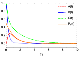
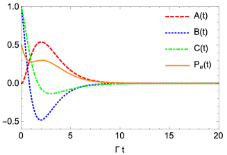
Figure 2: The plots of $A(t)$, $B(t)$, $C(t)$, and $P_{e}(t)$ for $\kappa=1$, $\Delta_{0}=0$ and $P_{e}(0)=0.5$. Left: regular case $\alpha=9.5$. Right: singular case $\alpha=1$.

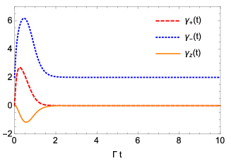
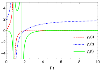
Figure 3: The plots of $\gamma_{+}(t)$, $\gamma_{-}(t)$, and $\gamma_{z}(t)$ for $\Gamma=1$, $\kappa=1$, $\Delta_{0}=0$. Left: regular case $\alpha=9.5$. Right: singular case $\alpha=1$.

Proposition 5

One has the following asymptotic behaviour for $\gamma_{\pm}(t)$ and $\gamma_{z}(t)$:

• for $\alpha\geq 1$

  $$\lim_{t\to\infty}\gamma_{+}(t)=\lim_{t\to\infty}\gamma_{z}(t)=0\ ,\ \ \ \lim_{t\to\infty}\gamma_{-}(t)=2\Gamma$$ (74)

• for $\alpha\in(0,1)$

  $$\lim_{t\to\infty}\gamma_{+}(t)=0\ ,\ \ \ \lim_{t\to\infty}\gamma_{z}(t)=\frac{1}{4}\Gamma(1-\alpha)\ ,\ \ \ \lim_{t\to\infty}\gamma_{-}(t)=\Gamma(1+\alpha).$$ (75)

It implies that asymptotically one has

• for $\alpha\geq 1$

  $$\mathcal{L}_{t}(\rho)\ \to\ {\Gamma}\left(\sigma_{-}\rho\sigma_{+}-\frac{1}{2}\{\sigma_{+}\sigma_{-},\rho\}\right)$$ (76)

• for $\alpha\in(0,1)$

  $$\mathcal{L}_{t}(\rho)\ \to\ \frac{\Gamma(1+\alpha)}{2}\left(\sigma_{-}\rho\sigma_{+}-\frac{1}{2}\{\sigma_{+}\sigma_{-},\rho\}\right)+\frac{\Gamma(1-\alpha)}{8}(\sigma_{z}\rho\sigma_{z}-\rho).$$ (77)

Let us note that the asymptotic evolution of coherence governed by (76) and (77) is the same. For details cf. Appendix E.

VI.2 Off-resonant case $\Delta_{0}\neq 0$

Now, the formulae for $A(t)$, $B(t)$, and $C(t)$ are much more involved and we were not able to find analytical condition for $\{\Delta_{0},\Gamma,\Gamma_{p}\}$ which guaranties invertible dynamical map $\Lambda_{t}$. We observe that contrary to the resonant case $B(t)$ may vanish at several moments of time which makes the generator even more singular than in the resonant case. Figure 4 shows that increasing $\Delta_{0}$ from ‘0’ (resonant case) to $\Delta_{0}=1.5$ one creates additional singular points for $\kappa=1$ and $\alpha=1.5$. However, if $\Delta_{0}=2.5$ all singularities are removed. Second interesting observation is related to indicators of non-Markovianity. In the resonant case if the generator is free from singularities (i.e. $\alpha\geq 8\kappa+1$) the evolution satisfies BLP condition and hence does not display information backflow. It is no longer true if $\Delta_{0}\neq 0$. Figure 5 shows that even if the generator is free from singularities the validity of BLP condition still depends for a given $\kappa$ on the parameters $\{\Delta_{0},\alpha\}$. Since $\gamma_{+}(t)$ might be negative, it is clear, that even if the dynamics satisfies BLP condition it needs not be P-divisible (cf. Theorem 1). Therefore, in the off-resonant case these two indicators, that is, P-divisibility and BLP condition do not coincide. This observation is quite interesting since in majority of studied examples these two notions coincide. It simply means that for off-resonant evolution the monotonicity condition

$$\frac{d}{dt}\|\Lambda_{t}(X)\|_{1}\leq 0,$$ (78)

is violated even if it is satisfied for all traceless Hermitian operators (i.e. $X\sim\rho_{1}-\rho_{2}$). This analysis shows that no information backflow does not guarantee the existence of positive trace-preserving propagators $V_{t,s}$. Actually, one may violate not only BLP condition but much weaker condition based on the geometric indicator LPP13 which measures the volume of accessible states. One finds that if the evolution is Markovian then

$$\frac{d}{dt}|{\rm det}\Lambda_{t}|=\frac{d}{dt}|\lambda_{1}(t)\lambda_{2}(t)\lambda_{3}(t)|\,\leq\,0,$$ (79)

where $\lambda_{k}(t)$ denote eigenvalues of the dynamical map ($k=1,2,3$). This condition is equivalent to (49) Sabrina-NJP , which is much weaker than BLP condition. The geometric and the BLP criteria of non-Markovianity are shown in Fig. 6. One sees that for parameters indicated in the left panel of Figure 6 this condition is violated proving that evolutions display strong memory effects. Finally, let us note that Fig. 5 shows that for the chosen values of parameters the rates oscillate with decreasing amplitudes around their asymptotic values, namely $\gamma_{+}(t)$ and $\gamma_{z}(t)$ oscillate around zero, and $\gamma_{-}(t)$ around $2\Gamma$. Interestingly, whenever $\gamma_{+}(t)$ is zero $\gamma_{z}(t)$ is also equal to zero, and $\gamma_{-}(t)$ is equal to $2\Gamma$, so for these moments $\mathcal{L}_{t}=\mathcal{L}$.

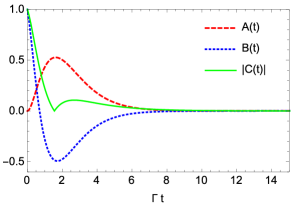
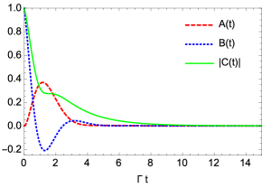
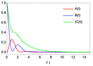
Figure 4: The plots of $A(t)$, $B(t)$, and $|C(t)|$ for $\kappa=1$, $\Gamma=1$, and $\alpha=1.5$. Left: $\Delta_{0}=0$. Center: $\Delta_{0}=1.5$. Right: $\Delta_{0}=2.5$.

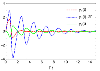
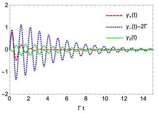
Figure 5: The plots of $\gamma_{+}(t)$, $\gamma_{-}(t)-2\Gamma$, and $\gamma_{z}(t)$ for $\kappa=1$, $\Gamma=1$, and $\alpha=1.5$. Left: $\Delta_{0}=3.0$ — BLP condition is violated. Right: $\Delta_{0}=6.5$ — BLP condition is satisfied.

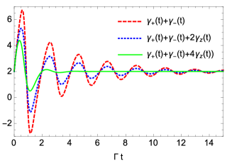
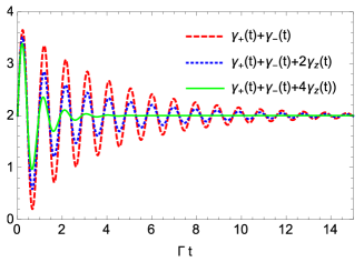
Figure 6: The plots of $\gamma_{+}(t)+\gamma_{-}(t)$, $\gamma_{+}(t)+\gamma_{-}(t)+2\gamma_{z}(t)$, and $\gamma_{+}(t)+\gamma_{-}(t)+4\gamma_{z}(t)$ for $\kappa=1$, $\Gamma=1$, $\alpha=1.5$. Left: $\Delta_{0}=3.0$. Right: $\Delta_{0}=6.5$.

VII Conclusion

We provided a detailed discussion of the evolution of a qubit interacting with single-photon wave packet. Clearly, this problem was already analyzed by several researchers (see e.g. WMSS11 ; SAL10a ; Francesco ; Branczyk ). In this paper it is shown that a set of hierarchical equations, already derived in GEPZ98 ; BCBC12 ; DSC17 ; DSC19 ; D20 , is equivalent to a single time-local master equation for the qubit density operator. To show this equivalence we make use of the general form of solution to this set defining a dynamical map $\{\Lambda_{t}\}_{t\geq 0}$ for an arbitrary photon profile $\xi(t)$. The price one pays for this reduction is highly nontrivial structure of time-dependent rates in the time-local master equation. Interestingly, the corresponding time-local generator has a structure of phase covariant generator which has been already extensively studied SKHD16 ; Sabrina-2016 ; Sabrina-NJP ; Francesco ; HSH19 ; Sergey-2020 . We provided the formulae for time dependent rates governing damping (cooling), heating and decoherence processes. These rates are fully controlled by the photon profile $\xi(t)$ which is a key ingredient of the entire analysis. It turn out that temporal correlations encoded into $\xi(t)$ give rise to all characteristic non-Markovian memory effects of the corresponding qubit evolution. Due to the interaction with a non-locally (in time) entangled field the system undergoes such phenomena as recoherence. But the recoherence is not universal, for some parameters the photon becomes only the source of decoherence.

Note that a dynamical map $\{\Lambda_{t}\}_{t\geq 0}$ representing the qubit evolution might be non-invertible for some time moments which implies the singularity of transition rates in the corresponding time-local master equation. The phenomenon of non-invertible maps were already considered in quantum optics for example in Cresser1 ; Cresser2 ; SKHD16 . Similar observation for phase covariant dynamics was also recently reported in Francesco . It should be stressed that being singular the time-local generator $\mathcal{L}_{t}$ gives rise to perfectly regular evolution D20 (represented by $\{\Lambda_{t}\}_{t\geq 0}$). Non-invertible dynamical maps were recently analyzed in PRL-2018 and CC19 in connection to divisibility (cf. also recent paper Jyrki-2021 ). Divisibility which is equivalent to the existence of a propagator $V_{t,s}$ is always guaranteed for invertible maps. For maps which are not invertible divisibility holds only under additional conditions PRL-2018 .

We provided the detailed analysis of the exponential profile. In particular we derived the formula for the maximal excitation probability. Such formula was also derived in a recent paper Branczyk via different methods. For exponential profile we derived explicit formulae for all time dependent rates of the time-local generator. The key observation is that for the exponential profile qubit evolution is never Markovian (i.e. CP-divisible). Interestingly, in the resonant case the dynamical map $\{\Lambda_{t}\}_{t\geq 0}$ is either invertible or looses invertibility in at most two moments of time. However, whenever it is invertible the evolution satisfies BLP condition which guarantees no information backflow. Off-resonant scenario is much more intricate since the number of singular points for the time-local generator highly depends upon the detuning parameter $\Delta_{0}$. Still, one can observe some universal properties of qubit dynamics. In particular $\gamma_{+}(t)\gamma_{z}(t)\leq 0$ for all $t\geq 0$. It shows that for any $t$ one of the transition rate is strictly negative and hence the dynamics is eternally non-Markovian Erika . Similar analysis was performed for a square pulse $\xi(t)$. The conclusions are very similar and they are not included in the manuscript.

Beyond exponential profile it is still possible to observe universal properties. We shown that in the resonant case assuming $\xi(t)\in\mathbb{R}_{+}$ the evolution satisfies BLP condition whenever it is invertible. Still the evolution is eternally non-Markovian ($\gamma_{z}(t)\leq 0$) but invertibility protects the system against the information backflow. This observation clearly shows that being invertible is not only a mathematical curiosity but implies direct physical consequences.

The problem of non-Markovian dynamics of the qubit interacting with a single-photon field was studied in Francesco by making use an infinite waveguide in the real-space approach. Authors of Francesco analyzed an exponential profile in resonance and $\kappa=\frac{1}{2}$. We consider off resonant case as well and allow for $\kappa\in[0,1]$. Moreover, we derive general properties for an arbitrary profile satisfying $\xi(t)\in\mathbb{R}_{+}$. In particular it is shown that in the resonant case whenever the dynamical map is invertible the evolution satisfies BLP condition meaning there is no information backflow. Exponential profile is just an example of this general property.

The system we consider provides a perfect platform to test and compare various aspects of non-Markovianity. Detailed analysis of the exponential profiles shows that the evolution of the qubit is never Markovian (CP-divisible). Moreover, it is eternally non-Markovian Erika , that is, one of the transition rate is always negative. We claim that the same holds for an arbitrary profile meaning that the interaction with a single-photon field always results in the eternally non-Markovian dynamics. In our opinion this is the first proper physical model displaying such non-trivial behavior. The analysis of non-Markovian dynamics of the system interacting with single-photon state is of particular importance for effective control of quantum systems and the storage and retrieving of quantum information. It would be interesting using similar theoretical methods to analyze the memory effects of a qubit interacting with $N$-photon field (the corresponding hierarchical equation were already derived in DSC19 ).

Appendix A Solution of hierchical equations

The solution to (16)-(18) reads as

$${\varrho}^{01}(t)=\left(\begin{array}[]{ccc}E(t)\rho_{eg}(0)&&F(t)P_{e}(0)+G(t)\\ 0&&-E(t)\varrho_{eg}(0)\end{array}\right)$$ (82)

$${\varrho}^{00}(t) =\left(\begin{array}[]{ccc}1-P_{e}(0)e^{-\Gamma t}&&\varrho_{ge}(0)e^{-\left(i\Delta_{0}+\frac{\Gamma}{2}\right)t}\\ \varrho_{eg}(0)e^{\left(i\Delta_{0}-\frac{\Gamma}{2}\right)t}&&P_{e}(0)e^{-\Gamma t}\end{array}\right)$$ (85)

$$E(t)=\sqrt{\kappa\Gamma}e^{-\Gamma t}\int_{0}^{t}ds\xi^{\ast}(s)e^{\left(i\Delta_{0}+\frac{\Gamma}{2}\right)s},$$ (86)

$$F(t)=2\sqrt{\kappa\Gamma}e^{-\left(i\Delta_{0}+\frac{\Gamma}{2}\right)t}\int_{0}^{t}ds\xi^{\ast}(s)e^{\left(i\Delta_{0}-\frac{\Gamma}{2}\right)s},$$ (87)

$$G(t)=-\sqrt{\kappa\Gamma}\int_{0}^{t}ds\xi^{\ast}(s)e^{\left(i\Delta_{0}+\frac{\Gamma}{2}\right)(s-t)},$$ (88)

and $\varrho^{10}(t)=\left(\varrho^{01}(t)\right)^{\dagger}$.

Appendix B Proof of Proposition 1

The proof is very simple: let $\tilde{\xi}(t)=e^{-i\omega_{c}t}\xi(t)\in\mathbb{C}$. Assuming $\rho(0)=|g\rangle\langle g|$ one obtains

$$P_{e}(t)=\kappa\Gamma e^{-\Gamma t}\left|\int_{0}^{t}ds\tilde{\xi}(s)e^{\left(i\omega_{0}+\frac{\Gamma}{2}\right)s}\right|^{2}.$$ (89)

To maximize this expression one has to maximize

$$\left|\int_{0}^{t}ds\tilde{\xi}(s)e^{\left(i\omega_{0}+\frac{\Gamma}{2}\right)s}\right|^{2}=|\langle\tilde{\xi}|f\rangle_{t}|^{2}$$ (90)

where the function $f(s)=e^{\left(-i\omega_{0}+\frac{\Gamma}{2}\right)s}$, and we introduce an inner product

$$\langle\tilde{\xi}|f\rangle_{t}:=\int_{0}^{t}\tilde{\xi}(s)f^{\ast}(s)ds.$$ (91)

It is evident that it is maximized for the profile $\tilde{\xi}(s)$ which is parallel to $f(s)$, that is, $\tilde{\xi}(s)=c(t)f(s)$, where $c(t)$ is a constant (depending on a fixed time $t$), and

$$\langle\tilde{\xi}|\tilde{\xi}\rangle_{t}=1.$$ (92)

This normalization condition allows to calculate $c(t)$ leading to

$$\tilde{\xi}(\tau)=\sqrt{\frac{\Gamma}{e^{\Gamma t}-1}}\,e^{\left(-i\omega_{0}+\frac{\Gamma}{2}\right)\tau}$$ (93)

for $\tau\in[0,t]$, and $\tilde{\xi}(\tau)=0$ for $\tau>t$ and then to (37). Clearly, the maximum excitation is realized at resonance $\omega_{c}=\omega_{0}$, i.e. $\Delta_{0}=0$. $\Box$

Appendix C Proof to Proposition 2

Let us assume that

$$\Delta_{0}=0,\ \ B(t)>0\ \ \mathrm{and}\ \ \xi(t)\in\mathbb{R}_{+}\ \ \mathrm{for\ \ all}\ \ t\geq 0.$$ (94)

One can check that then

$$\dot{A}(t)B(t)-\dot{B}(t)A(t)=2\kappa\Gamma\xi(t)e^{-\frac{\Gamma t}{2}}\left[B(t)\int_{0}^{t}ds\xi(s)e^{\frac{\Gamma s}{2}}+2A(t)\int_{0}^{t}ds\xi(s)e^{-\frac{\Gamma s}{2}}\right]\geq 0,$$ (95)

therefore $\gamma_{+}(t)\geq 0$ for all $t\geq 0$. In the next step one can find that

$$\gamma_{-}(t)=2\Gamma-4\kappa\Gamma\xi(t)e^{-\frac{\Gamma t}{2}}\frac{B(t)\int_{0}^{t}ds\xi(s)e^{\frac{\Gamma s}{2}}+2\left(A(t)-1\right)\int_{0}^{t}ds\xi(s)e^{-\frac{\Gamma s}{2}}}{B(t)}$$ (96)

and show that

$$B(t)\int_{0}^{t}ds\xi(s)e^{\frac{\Gamma s}{2}}+2\left(A(t)-1\right)\int_{0}^{t}ds\xi(s)e^{-\frac{\Gamma s}{2}}\leq 0,$$ (97)

which can be written in the form

$$\left[1-4\kappa\Gamma\int_{0}^{t}ds\xi(s)e^{\frac{\Gamma s}{2}}\int_{0}^{s}d\tau\xi(\tau)e^{-\frac{\Gamma\tau}{2}}+2\kappa\Gamma\int_{0}^{t}ds\xi(s)e^{\frac{\Gamma s}{2}}\int_{0}^{t}ds\xi(s)e^{-\frac{\Gamma s}{2}}\right]$$

$$\times e^{-\Gamma t}\int_{0}^{t}ds\xi(s)e^{\frac{\Gamma s}{2}}-2\int_{0}^{t}ds\xi(s)e^{-\frac{\Gamma s}{2}}\leq 0.$$ (98)

This inequality can be proved by using

$$e^{-\Gamma t}\int_{0}^{t}ds\xi(s)e^{\frac{\Gamma s}{2}}\leq\int_{0}^{t}ds\xi(s)e^{-\frac{\Gamma s}{2}},$$ (99)

which follows from

$$e^{-\Gamma t}\int_{0}^{t}ds\xi(s)e^{\frac{\Gamma s}{2}}\leq e^{-\frac{\Gamma t}{2}}\int_{0}^{t}ds\xi(s)\leq\int_{0}^{t}ds\xi(s)e^{-\frac{\Gamma s}{2}}$$ (100)

and by applying

$$2\kappa\Gamma\int_{0}^{t}ds\xi(s)e^{\frac{\Gamma s}{2}}\int_{0}^{t}ds\xi(s)e^{-\frac{\Gamma s}{2}}<1+4\kappa\Gamma\int_{0}^{t}ds\xi(s)e^{\frac{\Gamma s}{2}}\int_{0}^{s}d\tau\xi(\tau)e^{-\frac{\Gamma\tau}{2}}.$$ (101)

Let us notice that on both sides of the last inequality we deal with non-decreasing functions of $t$ and one can prove it by comparing values of these function at $t=0$ and their derivatives. Hence we obtain that $\gamma_{-}(t)\geq 2\Gamma$ for all $t\geq 0$.

Now we show that if (94) holds, then $C(t)>0$. Let us notice that from

$$1-4\kappa\Gamma\int_{0}^{t}ds\xi(s)e^{\frac{\Gamma s}{2}}\int_{0}^{s}d\tau\xi(\tau)e^{-\frac{\Gamma\tau}{2}}>0,$$ (102)

which follows from $B(t)>0$, and

$$\int_{0}^{t}ds\xi(s)e^{\frac{\Gamma s}{2}}\int_{0}^{s}d\tau\xi(\tau)e^{-\frac{\Gamma\tau}{2}}=-\int_{0}^{t}ds\xi(s)e^{-\frac{\Gamma s}{2}}\int_{0}^{s}d\tau\xi(\tau)e^{\frac{\Gamma\tau}{2}}+\int_{0}^{t}ds\xi(s)e^{-\frac{\Gamma s}{2}}\int_{0}^{t}ds\xi(s)e^{\frac{\Gamma s}{2}}$$ (103)

we obtain

$$1-2\kappa\Gamma\int_{0}^{t}ds\xi(s)e^{-\frac{\Gamma s}{2}}\int_{0}^{s}ds\xi(\tau)e^{\frac{\Gamma\tau}{2}}>\;\;\;\;$$

$$2\kappa\Gamma\left(2\int_{0}^{t}ds\xi(s)e^{-\frac{\Gamma s}{2}}\int_{0}^{t}ds\xi(s)e^{\frac{\Gamma s}{2}}-3\int_{0}^{t}ds\xi(s)e^{-\frac{\Gamma s}{2}}\int_{0}^{s}d\tau\xi(\tau)e^{\frac{\Gamma\tau}{2}}\right).$$ (104)

To check that

$$\int_{0}^{t}ds\xi(s)e^{-\frac{\Gamma s}{2}}\int_{0}^{t}ds\xi(s)e^{\frac{\Gamma s}{2}}\geq\frac{3}{2}\int_{0}^{t}ds\xi(s)e^{-\frac{\Gamma s}{2}}\int_{0}^{s}d\tau\xi(\tau)e^{\frac{\Gamma\tau}{2}}$$ (105)

we can use the fact that on both sides of the above inequality we deal with non-decreasing functions of $t$ having the same values for $t=0$ whose derivatives satisfies the inequality

$$\xi(t)e^{-\frac{\Gamma t}{2}}\int_{0}^{t}ds\xi(s)e^{\frac{\Gamma s}{2}}+\xi(t)e^{\frac{\Gamma t}{2}}\int_{0}^{t}ds\xi(s)e^{-\frac{\Gamma s}{2}}\geq\frac{3}{2}\xi(t)e^{-\frac{\Gamma t}{2}}\int_{0}^{t}ds\xi(s)e^{\frac{\Gamma s}{2}}.$$ (106)

Hence $C(t)>0$ for all $t\geq 0$. Using this results one can easily show that

$$\dot{C}(t)=-\frac{\Gamma}{2}C(t)-2\kappa\Gamma e^{-\Gamma t}\xi(t)\int_{0}^{t}ds\xi(s)e^{\frac{\Gamma s}{2}}<0$$ (107)

so we see that $\gamma_{+}(t)+\gamma_{-}(t)+4\gamma_{z}(t)>0$ is satisfied for all $t\geq 0$.

Finally let us derive

$$\dot{B}(t)C(t)-2B(t)\dot{C}(t)=4\kappa\Gamma\xi(t)e^{-\frac{\Gamma t}{2}}\left[B(t)e^{-\frac{\Gamma t}{2}}\int_{0}^{t}ds\xi(s)e^{\frac{\Gamma s}{2}}-C(t)\int_{0}^{t}ds\xi(s)e^{-\frac{\Gamma s}{2}}\right].$$ (108)

To prove that this expression is less or equal to zero one can use the properties (103), (105), and (100). This property leads to $\gamma_{z}(t)\leq 0$ for all $t\geq 0$ and ends the proof. $\Box$

Appendix D Proof to Proposition 4

Assuming $\rho(0)=|g\rangle\langle g|$ one has

$$P_{e}(\alpha,\Delta_{0},t)=\frac{4\kappa\alpha\Gamma^{2}}{(1-\alpha)^{2}\Gamma^{2}+4\Delta_{0}^{2}}\left(e^{-\Gamma t}-2e^{-\frac{(1+\alpha)\Gamma t}{2}}\cos\Delta_{0}t+e^{-\alpha\Gamma t}\right).$$ (109)

Introducing $\chi$ such that $\Gamma t/2=\chi$ one finds that the function

$$P_{e}=f(\alpha,\Delta_{0},\chi)=\frac{4\kappa\alpha\Gamma^{2}}{(1-\alpha)^{2}\Gamma^{2}+4\Delta_{0}^{2}}\left(e^{-2\chi}-2e^{-(1+\alpha)\chi}\cos\Delta_{0}t+e^{-\alpha\chi}\right).$$ (110)

attains its local maximum for $\alpha=1$, $\Delta_{0}=0$, and $\chi=1$ which corresponds to $t=2/\Gamma$. Finally,

$$\lim_{\alpha\to 1}f(\alpha,0,1)=\frac{4\kappa}{e^{2}},$$ (111)

which ends the proof. $\Box$

Appendix E formulae for $\gamma_{+}$, $\gamma_{-}$, and $\gamma_{z}$ for $\Delta_{0}=0$

If $\alpha\neq 1$, then for (67)-(69) we obtain

$$\gamma_{+}(t) =16\alpha\Gamma\kappa e^{-\frac{1}{4}(\alpha+1)\Gamma t}\sinh\left[\frac{1}{4}(\alpha-1)\Gamma t\right]\frac{\left(\alpha^{2}-16\kappa-1\right)\sinh\left[\frac{\alpha\Gamma t}{2}\right]+\left(\alpha^{2}-1\right)\cosh\left[\frac{\alpha\Gamma t}{2}\right]+16\alpha\kappa\sinh\left[\frac{\Gamma t}{2}\right]}{(\alpha-1)\left\{8\kappa(1-\alpha)+16\alpha\kappa e^{\frac{1}{2}(\alpha+1)\Gamma t}+(\alpha+1)(\alpha-8\kappa-1)e^{\alpha\Gamma t}\right\}},$$ (112)

$$\gamma_{-}(t) =-\gamma_{+}(t)+\frac{2(\alpha+1)\Gamma\left\{8\kappa(1-\alpha)+8\alpha\kappa e^{\frac{1}{2}(\alpha+1)\Gamma t}+(\alpha-8\kappa-1)e^{\alpha\Gamma t}\right\}}{8\kappa(1-\alpha)+16\alpha\kappa e^{\frac{1}{2}(\alpha+1)\Gamma t}+(\alpha+1)(\alpha-8\kappa-1)e^{\alpha\Gamma t}},$$ (113)

$$\gamma_{z}(t) =-\frac{1}{4}(\gamma_{+}(t)+\gamma_{-}(t))-\frac{\Gamma\left\{-8\alpha(\alpha+2)\kappa e^{\frac{\alpha\Gamma t}{2}}+4(\alpha+1)(2\alpha+1)\kappa e^{\frac{\Gamma t}{2}}-(\alpha-1)(\alpha-4\kappa+1)e^{\left(\alpha+\frac{1}{2}\right)\Gamma t}\right\}}{16\alpha\kappa e^{\frac{\alpha\Gamma t}{2}}-8(\alpha+1)\kappa e^{\frac{\Gamma t}{2}}+2(\alpha-1)(\alpha-4\kappa+1)e^{\left(\alpha+\frac{1}{2}\right)\Gamma t}}.$$ (114)

For $\alpha=1$, from (70)-(72) we get

$$\gamma_{+}(t) =\frac{4\Gamma^{2}\kappa t\Big{\{}2\kappa(\Gamma t+2)+e^{\Gamma t}\big{[}2\kappa(\Gamma t-2)-1\big{]}\Big{\}}}{4\kappa e^{\Gamma t}+e^{2\Gamma t}(4\kappa(\Gamma t-1)-1)}$$ (115)

$$\gamma_{-}(t) =-\gamma_{+}(t)+\frac{2\Gamma\Big{\{}8\kappa+e^{\Gamma t}\big{[}4\kappa(\Gamma t-2)-1\big{]}\Big{\}}}{4\kappa+e^{\Gamma t}(4\kappa(\Gamma t-1)-1)}$$ (116)

$$\gamma_{z}(t) =-\frac{1}{4}(\gamma_{+}(t)+\gamma_{-}(t))+\frac{\Gamma}{2}\left[\frac{4\Gamma\kappa t}{2(\kappa+\Gamma\kappa t)+(1-2\kappa)e^{\Gamma t}}+1\right]$$ (117)

Hence one can find the limits (76) and (77).

Appendix F Proof to Proposition 4

One can rewrite (68) as

$$B(t)=\frac{16\kappa\alpha}{\alpha^{2}-1}e^{-\frac{1+\alpha}{2}\Gamma t}+\left(1-\frac{8\kappa}{\alpha-1}\right)e^{-\Gamma t}-\frac{8\kappa}{\alpha+1}e^{-(1+\alpha)\Gamma t}$$ (118)

If $\alpha<1$, then we rewrite the above as:

$$B(t)=e^{-\frac{1+\alpha}{2}\Gamma t}\left(\frac{16\kappa\alpha}{\alpha^{2}-1}+\left(1-\frac{8\kappa}{\alpha-1}\right)e^{-\frac{1-\alpha}{2}\Gamma t}-\frac{8\kappa}{\alpha+1}e^{-\frac{1+\alpha}{2}\Gamma t}\right)$$ (119)

The limit of the second factor is $16\kappa\alpha/(\alpha^{2}-1)<0$, hence $B(t)$ is negative for $t$ large enough. Because $B(0)=1$, there exists $t$ such that $B(t)=0$.

If $\alpha\in(1,8\kappa+1)$, then rewriting (118) as:

$$B(t)=e^{-\Gamma t}\left(\frac{16\kappa\alpha}{\alpha^{2}-1}e^{-\frac{\alpha-1}{2}\Gamma t}+\left(1-\frac{8\kappa}{\alpha-1}\right)-\frac{8\kappa}{\alpha+1}e^{-\alpha\Gamma t}\right)$$ (120)

one can notice that the limit of the second factor is $1-8\kappa/(\alpha-1)$ which now is negative due to assumption about the range of $\alpha$ and again there exists $t$ such that $B(t)=0$.

If $\alpha=1$, then the second factor in (71) is equal 1 for $t=0$ and it is unbounded from below, hence there exists $t$ such that $B(t)=0$ . Hence for the whole range $\alpha<8\kappa+1$ the dynamics is not invertible.

If $\alpha\geq 8\kappa+1$, then $1-8\kappa/(\alpha-1)\geq 0$ and estimating (118) as follows:

$$B(t) =\frac{16\kappa\alpha}{\alpha^{2}-1}e^{-\frac{1+\alpha}{2}\Gamma t}+\left(1-\frac{8\kappa}{\alpha-1}\right)e^{-\Gamma t}-\frac{8\kappa}{\alpha+1}e^{-(1+\alpha)\Gamma t}$$

$$\geq\frac{16\kappa\alpha}{\alpha^{2}-1}e^{-\frac{1+\alpha}{2}\Gamma t}+\left(1-\frac{8\kappa}{\alpha-1}\right)e^{-\frac{1+\alpha}{2}\Gamma t}-\frac{8\kappa}{\alpha+1}e^{-(1+\alpha)\Gamma t}=\left(1+\frac{8\kappa}{\alpha+1}\right)x-\frac{8\kappa}{\alpha+1}x^{2}$$ (121)

where $x=\exp(-(1+\alpha)\Gamma t/2)\in(0,1]$, one can observe that the above expression is positive for $x\in(0,1]$, hence $B(t)$ is positive for all $t$.

Finally, using the result from Appendix C i.e whenever $B(t)>0$ then $C(t)>0$, we see that for the range $\alpha\geq 8\kappa+1$, we get $C(t)>0$, and we conclude that the dynamics is invertible.

References

• (1) Breuer H P and Petruccione F 2002 The Theory of Open Quantum Systems (Oxford: Oxford University Press)
• (2) Alicki R and Lendi K 1987 Quantum Dynamical Semigroups and Applications (Berlin: Springer)
• (3) Gorini V, Kossakowski A and Sudarshan E C G 1976 J. Math. Phys. 17 821
• (4) Lindblad G 1976 Comm. Math. Phys. 48 119
• (5) Breuer H P, Laine E M, Piilo J and Vacchini B 2016 Rev. Mod. Phys. 88 021002
• (6) de Vega I and Alonso D 2017 Rev. Mod. Phys. 89 015001
• (7) Li L, Hall M J W and Wiseman H M 2018 Phys. Rep. 759 1
• (8) Rivas Á, Huelga S F and Plenio M B 2014 Rep. Prog. Phys. 77 094001
• (9) Li C F, Guo G C and Piilo J 2000 EPL (Europhysics Letters) 127 50001
• (10) Li C F, Guo G C and Piilo J 2000 EPL (Europhysics Letters) 123 30001
• (11) Pollock F A, Rodríguez-Rosario C, Frauenheim T, Paternostro M and Modi K 2018 Phys. Rev. A 97 012127
• (12) Pollock F A, Rodríguez-Rosario C, Frauenheim T, Paternostro M and Modi K 2018 Phys. Rev. Lett. 120 040405
• (13) Milz S and Modi K 2021 PRX Quantum 2, 030201
• (14) Loudon R 2000 The Quantum Theory of Light third edition (Oxford: Oxford University Press)
• (15) Milburn G J 2008 Eur. Phys. J. Spec. Top. 159 113
• (16) Knill E, Laflamme R and Milburn G J 2001 Nature 409, 46
• (17) Ralph T C, Gilchrist A and Milburn G J 2003 Phys. Rev. A 68 042319
• (18) Dowling J 2008 J. Contemp. Phys. 49 125 (doi:10.1080/00107510802091298)
• (19) Munro W J, Nemoto K, Milburn G J and Beaustien S L 2002 Phys. Rev. A 66 023819
• (20) Scarani V, Bechmann-Pasquinucci H, Cerf N J, Dusek M, Lütkenhaus N N, Peev M 2009 Rev. Mod. Phys. 81 1301
• (21) S. Aaronson, A. Arkhipov, The computation complexity of linear optics. In Proc. 43rd Annual ACM Symposium on the Theory of Computing (STOC11), San Jose, CA, USA, 68 June 2011, pp. 333342. New York, NY: Association for Computing Machinery.
• (22) Cooper M, Wright L J, Söller C and Smith B J 2013 Opt. Express 21 5309
• (23) Peaudecerf B, Sayrin C, Zhou X, Rybarczyk T, Gleyzes S, Dotsenko I, Raimond J M, Brune M and Haroche S 2013 Phys. Rev. A 87, 042320
• (24) Reiserer A and Rempe G 2015 Rev. Mod. Phys. 87 1379
• (25) Leong V, Seidler M A, Steiner M, Ceré A and Kurtsiefer Ch 2016 Nat. Commun. 7 13716
• (26) Lodahl P, Mahmoodian S, Stobbe S, Rauschenbeutel A, Schneeweiss P, Volz J, Pichler H and Zoller P 2017 Nature 541 473
• (27) Gardiner C W and Collet M J 1985 Phys. Rev. A 31 3761
• (28) Gheri M K, Ellinger K, Pellizzari T, and Zoller P 1998 Fortschr. Phys. 46 4-5 401
• (29) Wang Y, Minář J, Sheridan L and Scarani V 2011 Phys. Rev. A 83 063842
• (30) Baragiola B Q, Cook R L, Brańczyk A M, and Combes J 2012 Phys. Rev. A 86 013811
• (31) J. E. Gough, M. R. James, H. I. Nurdin, and J. Combes, Phys. Rev. A 86, 043819 (2012).
• (32) B. Q. Baragiola, and J. Combes, Phys. Rev. A 96, 023819 (2017).
• (33) Dąbrowska A, Sarbicki G, and Chruściński D 2017 Phys. Rev. A 96 053819
• (34) Dąbrowska A, Sarbicki G, and Chruściński D 2019 Phys. A: Math. Theor. 52 105303
• (35) Dąbrowska A 2020 J. Opt. Soc. Am. B 37 1240
• (36) Smirne A, Kołodyński J, Huelga S F and Demkowicz-Dobrzański R 2016 Phys. Rev. Lett. 116 120801
• (37) Lankinen J, Lyyra H, Sokolov B, Teittinen J, Ziaei B, and Maniscalco S 2016 Phys. Rev. A 93 052103
• (38) Teittinen J, Lyyra H, Sokolov B, and Maniscalco S 2018 New J. Phys. 20 073012
• (39) Fang Y L, Ciccarello F, and Baranger H U 2018 New J.Phys. 20 043035
• (40) Haase J F, Smirne A, and Huelga S F in Advances in Open Systems and Fundamental Tests of Quantum Mechanics edited by B. Vacchini, H.-P. Breuer, and A. Bassi, Springer Proceedings in Physics 237, 41-57 (2019).
• (41) Filippov S N, Glinov A N, and Leppäjärvi L 2020 Lobachevskii Journal of Mathematics 41 617
• (42) Andersson E, Cresser J D and Hall M J W 2007 J. Mod. Opt. 54 1695
• (43) Cresser J D and Facer C 2010 Opt. Commun. 283 773
• (44) Hou S C, Yi X X , Yu S X, and Oh C H 2012 Phys. Rev. A 86 012101
• (45) Chruściński D, Rivas Á and Størmer E 2018 Phys. Rev. Lett. 121 080407
• (46) Chakraborty S and Chruściński D 2019 Phys. Rev. A 99 042105
• (47) Hegde A S, Athulya K P, Pathak V, Piilo J, Shaji A Open Quantum Dynamics with Singularities: Master Equations and Degree of Non-Markovianity, arXiv:2105.12505
• (48) Hall M J W, Cresser J D, Li Li, and Andersson E 2014 Phys. Rev. A 89 042120
• (49) Chruściński D, Kossakowski A and Rivas Á 2011 Phys. Rev. A 83 052128
• (50) Bylicka B, Johansson M and Acín A 2017 Phys. Rev. Lett. 118 120501
• (51) Buscemi F and Datta N 2016 Phys. Rev. A 93 012101
• (52) De Santis D, Johansson M, Bylicka B, Bernardes N K and Acín A, 2020 Phys. Rev. A 102 012214
• (53) De Santis D and Johansson M 2020 New J. Phys. 22 093034
• (54) Chakraborty U and Chruściński D 2021 New J. Phys. 23 013009
• (55) Rivas Á, Huelga S F, and Plenio M B 2010 Phys. Rev. Lett. 105 050403
• (56) Breuer H P, Laine E M, and Piil J 2009 Phys. Rev. Lett. 103 210401
• (57) Megier N, Chruściński D, Piilo J, and Strunz W T 2017 Scientific Reports 7 6379
• (58) Siudzińska and Chruściński D 2020 J. Phys. A: Math. Theor. 53 375305
• (59) Smirne A, Egloff D, Díaz M G, Plenio M B, and Huelga S F 2019 Quantum Sci. Technol. 4 01LT01
• (60) Milz S, Egloff D, Taranto P, Theurer T, Plenio M B, Smirne A, and Huelga S F 2020 Phys. Rev. X 10 041049
• (61) Luchnikov I A, Vintskevich S V, Ouerdane H, and Filippov S N 2019 Phys. Rev. Lett. 122 160401
• (62) Lorenzo S, Plastina F and Paternostro M 2013 Phys. Rev. A 88 020102(R)
• (63) Chruściński D, Macchiavello C and Maniscalco S 2017 Phys. Rev. Lett. 118 080404
• (64) Fischer K A Trivedi R Ramasesh V Siddiqi I and Vuc̆ković J 2018 Quantum 2 69
• (65) Gardiner C W and Zoller P 2010 Quantum noise (Springer-Verlag Berlin-Heidelberg)
• (66) F. Ciccarello, S. Lorenzo, V. Giovannetti, and G. M. Palma, arXiv:2106.11974
• (67) Witt B, Rudnicki Ł, Tanimura Y and Mintert F 2017 New J. Phys. 19 013007
• (68) Tanimura Y and Kubo R 1989 J. Phys. Soc. Japan 58 101
• (69) Chruściński D, Kossakowski A, and Pascazio S 2010 Phys. Rev. A 81 032101
• (70) Stobińska M, Alber G and Leuchs G, 2009 Euro. Phys. Lett. 86 14007
• (71) Rephaeli E, Jung-Tsung Shen, and Fan S 2010 Phys. Rev. A 82 033804
• (72) Rag H S and Gea-Banacloche J 2017 Phys. Rev. A 96 033817
• (73) Kimura G 2002 Phys. Rev. A 66 062113
• (74) Chruściński D, Kimura G, Kossakowski A, and Shishido Y 2021 Phys. Rev. Lett. 127 050401
• (75) Chruściński D, Fujii R , Kimura G, and Ohno H 2021 Lin. Alg. Appl. 630 293
• (76) Forn-Díaz P, Warren CW, Chang C W S, Vadiraj A M and Wilson C M 2017 Phys. Rev. Appl. 8 054015
• (77) Dinc F, Ercan I, and Brańczyk A M 2019 Quantum 3 213