The Fate of Shear-Oscillated Amorphous Solids

Abstract

The behavior of shear-oscillated amorphous materials is studied using a coarse-grained model. Samples are prepared at different degrees of annealing and then subject to athermal and quasistatic oscillatory deformations at various fixed amplitudes. The steady-state reached after several oscillations is fully determined by the initial preparation and the oscillation amplitude, as seen from stroboscopic stress and energy measurements. Under small oscillations, poorly annealed materials display shear-annealing, while ultra-stabilized materials are insensitive to them. Yet, beyond a critical oscillation amplitude, both kind of materials display a discontinuous transition to the same mixed state composed by a fluid shear-band embedded in a marginal solid. Quantitative relations between uniform shear and the steady-state reached with this protocol are established. The transient regime characterizing the growth and the motion of the shear band is also studied.

I Introduction

Amorphous solids are a vast class of materials, common in nature and ubiquitous for human applications. Their mechanical behaviour is strongly affected by the preparation protocol: poorly annealed materials, such as emulsions, foams or gels, are soft and ductile, while well annealed materials such as metallic glasses, ceramics and silica are hard and brittleBonn et al. (2017); Nicolas et al. (8 12). Under a uniform deformation, the former tend to melt into a liquid, while the latter fail with a sharp stress-drop and the appearance of a thin liquid shear-band Shi and Falk (2006); Ozawa et al. (2018); Popović, de Geus, and Wyart (2018); Barlow, Cochran, and Fielding (2020). Although we tend to distinguish between these two kind of yielding, a debate is open: ductile materials could also display stress overshootsBarlow, Cochran, and Fielding (2020); Ozawa et al. (2021); Richard, Rainone, and Lerner (2021); Fielding (2021). Beyond finite-size issuesOzawa et al. (2021); Richard, Rainone, and Lerner (2021); Fielding (2021), dealing only with transient states does not help to settle the discussion. This is where an oscillatory deformation protocolFiocco, Foffi, and Sastry (2014); Leishangthem, Parmar, and Sastry (2017); Das, Parmar, and Sastry (2020); Hexner, Liu, and Nagel (2020); Sastry (2021); Khirallah et al. (2021); Yeh et al. (2020); Kawasaki and Berthier (2016); Regev, Lookman, and Reichhardt (2013); Regev et al. (2015) becomes handy, since it opens the possibility of characterizing a transition in terms of stationary states. In molecular dynamics (MD) simulations, two different “phases” have been identified: For moderate strain amplitudes $\Gamma$, the material appears solid and is progressively annealedLeishangthem, Parmar, and Sastry (2017); Das, Parmar, and Sastry (2020); Yeh et al. (2020); Regev, Lookman, and Reichhardt (2013); Kawasaki and Berthier (2016) as oscillation cycles accumulate. Above a critical amplitude $\Gamma_{c}$, further shear-annealing is prevented and a shear-band coexists with a solidFiocco, Foffi, and Sastry (2013); Regev, Lookman, and Reichhardt (2013); Kawasaki and Berthier (2016); Leishangthem, Parmar, and Sastry (2017); Das, Parmar, and Sastry (2020). Despite a rapidly growing literatureFiocco, Foffi, and Sastry (2013); Regev, Lookman, and Reichhardt (2013); Fiocco, Foffi, and Sastry (2014); Regev et al. (2015); Kawasaki and Berthier (2016); Priezjev (2016, 2017); Leishangthem, Parmar, and Sastry (2017); Regev and Lookman (2017, 2018); Das, Parmar, and Sastry (2020); Mungan et al. (2019); Bhaumik, Foffi, and Sastry (2021); Parmar, Kumar, and Sastry (2019); Das, Vinutha, and Sastry (2020); Yeh et al. (2020); Hexner, Liu, and Nagel (2020); Sastry (2021); Khirallah et al. (2021), basic questions remain to be addressed: (i) the nature of the transition at $\Gamma_{c}$, (ii) the relation between steady-states in the two protocols (oscillatory and uniform shear), and (iii) how those states are reached.

To answer these questions, in this manuscript we use a coarse-grained approach, which goes beyond natural limitations of MD simulations. We find that the transition from solid to flow at $\Gamma_{c}$ is discontinuous. We quantitatively relate properties of the emerging phases in oscillatory shear with those of the uniform-deformation protocol. Moreover, we describe transient stages previously unexplored.

To do that, we prepare samples at different degrees of annealing, characterized by the initial energy $E_{\text{init}}$ per unit volume, and subject them to oscillatory deformations at various fixed amplitudes $\Gamma$ until steady-states are reached. We find that once a driving condition ($E_{\text{init}}$,$\Gamma$) is chosen, it univocally defines the material’s fate in the steady-state; allowing us to fill a sort of phase diagram. Very well-annealed samples ($E_{\text{init}}\!<\!E^{*}$, with $E^{*}$ a critical annealing level) are insensitive to small oscillations, while poorly-annealed samples ($E_{\text{init}}\!>\!E^{*}$) exhibit shear-annealing for large enough sub-critical $\Gamma$. We therefore distinguish between stable solids, that keep memory of their initial condition, and marginal solids which result from poorly-annealed samples loosing memory of their initial conditions due to the shear-annealing by oscillations. Yet, when the oscillation amplitude reaches the critical threshold $\Gamma_{c}(E_{\text{init}})$, every sample undergoes a discontinuous transition, comprising a jump in stress and energy, towards the same mixed solid-fluid state. Part of the system melt in a shear-band while the rest becomes a critical solid of energy $E^{*}$, independently on the initial condition. The fluid in the band corresponds to the one of the stationary state at large uniform quasi-static shear and holds at most the uniform yield stress $\Sigma_{y}$. As $\Gamma$ is further increased, the width of the shear-band scales as a power of $(\Gamma-\Sigma_{y}/\mathcal{G})$, with $\mathcal{G}$ the effective shear-modulus, further relating uniform and oscillatory protocols. Also, a rich transient dynamics towards the steady-state above $\Gamma_{c}$ is unveiled. We show a band-width growth as a function of the number of oscillation cycles that is reminiscent of critical domain coarsening. Surprisingly, once the band reaches its stable width it ballistically sweeps out the deeply-annealed regions, if present, turning them in the critical solid of energy $E^{*}$, and finally displays an (anomalous) diffusion. Overall, our manuscript offers answers to fresh issues raised by MD simulations of glasses.

II method

Our modelling is based on the evolution of a two-dimensional scalar strain field in a disordered potential, previously used to study yielding under uniform deformationJagla (2007); Fernández Aguirre and Jagla (8 07); Ferrero and Jagla (9 11); Jagla (2020); Ferrero and Jagla (2021). Initial sample annealing is achieved by tuning the configuration of the disordered landscape (lower initial energies $E_{\text{init}}$ for better annealed systems). Within this picture, the strain field behaves as a manifold propagating in a disorder mediumLin et al. (2014); Fernández Aguirre and Jagla (8 07); Ferrero and Jagla (9 11). Two essential ingredients are incorporated: the quadruple Eshelby’s elastic interactionEshelby (1957); Nicolas et al. (8 12) and a disorder that rather than originating in quenched impurities mimics the random positions of particles. The local disorder changes irreversibly, even if the strain manifold revisits the same location. Details of our method are presented in AppendixA.

III Results

In view of their relevance in interpreting the shear oscillation results, we first reproduce some key features in uniform shear. In Fig.1(a) we show stress-strain curves for individual samples prepared at different degrees of annealing $E_{\text{init}}$ (see also AppendixB). After an initial linear elastic response of slope $\mathcal{G}\approx 0.91$, all samples reach at large strain $\gamma\gtrsim 3$ a common plateau corresponding to the yield stress $\Sigma_{y}=0.375\pm 0.003$. The characteristic strain $\gamma_{y}$ where plasticity becomes important is estimated as $\gamma_{y}=\Sigma_{y}/\mathcal{G}\simeq 0.413$. Poorly annealed materials display a monotonic crossover from an elastic solid to a liquid crossing $\gamma_{y}$, while well annealed systems remain elastic above $\gamma_{y}$ up to a failure strain $\gamma_{\tt f}$ where a sharp stress downfall occurs. The overshoot gets larger for better annealed samplesOzawa et al. (2018); Popović, de Geus, and Wyart (2018); Barlow, Cochran, and Fielding (2020); Fielding (2021). In general, the total energy per volume of the material can be decomposed into two contributions: $E_{\rm tot}=E_{\tt sf}+\Sigma^{2}/(4\mu)$, where the second contribution is due to macroscopic elastic deformation (with $\mu=1/2$ the shear modulus) and $E_{\tt sf}$, called ‘stress-free energy’ afterward, characterizes the state of the material with zero macroscopic stress. In the large uniform shear limit $\gamma\rightarrow\infty$, where the memory of the initial state is completely erased, all samples converge to a homogeneous stationary liquid state with $E_{\tt sf}^{\tt stat}=-0.122\pm 0.001\equiv E_{\text{liq}}$ (see Fig.7 in AppendixB).

 

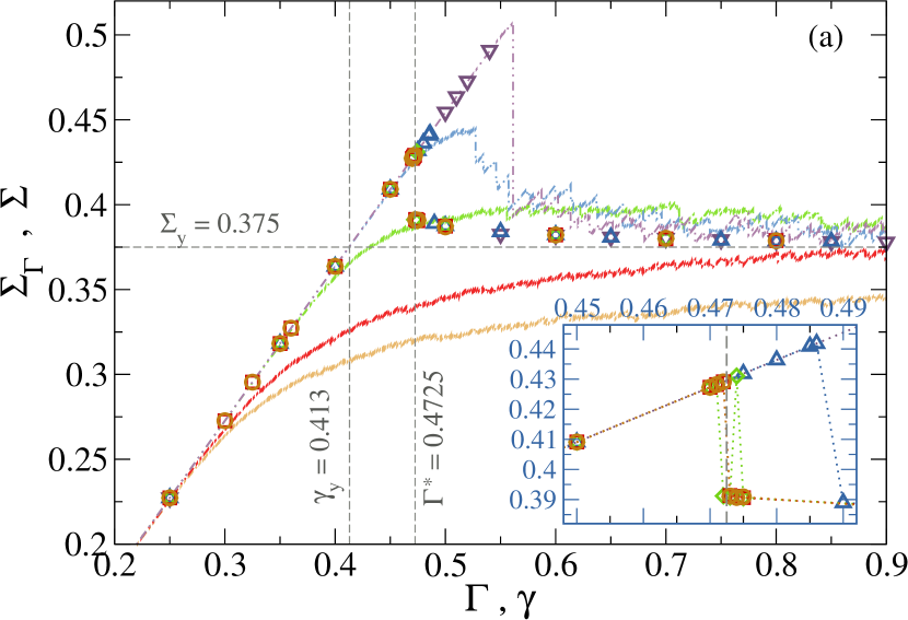
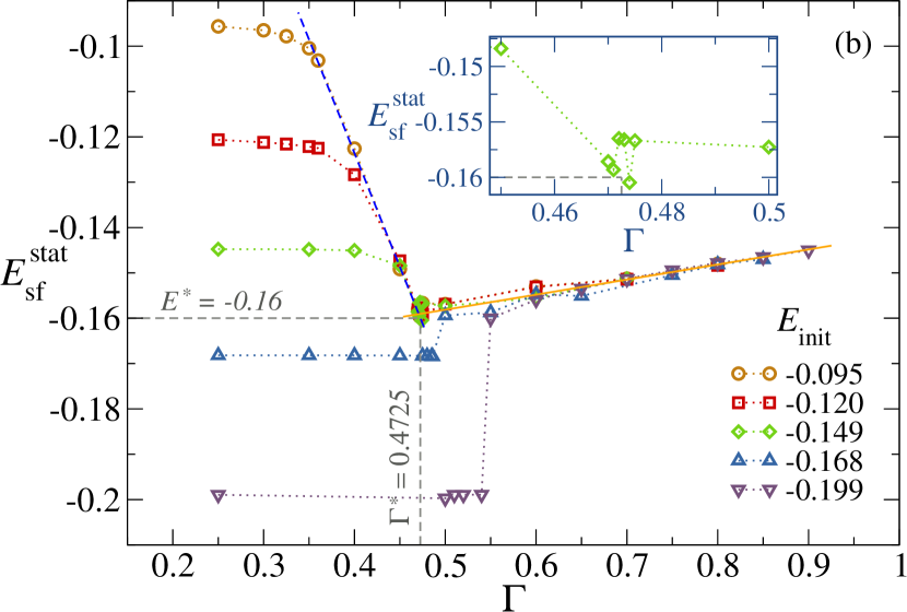
Figure 1: Stationary properties– (a) Symbols: Maximum stress $\Sigma_{\Gamma}$ versus the oscillatory strain amplitude $\Gamma$. Curves: Stress-strain ($\Sigma$ vs $\gamma$) produced by quasi-static uniform shear. Different colors code for different degrees of initial annealing, signaled in the bottom panel. The inset shows a zoom-in on the transition region. System size is $128^{2}$. (b) Stress-free steady energy $E_{\tt sf}^{\tt stat}$ versus the $\Gamma$. The purple dashed-line corresponds to “marginal solids”. The orange solid line displays a fit of $E_{\tt sf}^{\tt stat}(\Gamma)$ discussed in the text. The inset shows a zoom-in on the transition region (only $E_{\text{init}}=-0.149$ is shown).

III.1 Steady-state properties

Now, in our oscillatory protocol, the material is deformed by quasi-statically varying the strain from $0$ to $\Gamma$, then to $-\Gamma$ and subsequently back to $0$ to complete one cycle of amplitude $\Gamma$. This cycle is repeated until a steady-state is reached. By varying $\Gamma$ and $E_{\text{init}}$, we obtain an assortment of stationary states. Figure 1(a) shows the steady-state maximum stressLeishangthem, Parmar, and Sastry (2017); Fiocco, Foffi, and Sastry (2013); Yeh et al. (2020) $\Sigma_{\Gamma}=\frac{1}{2}(\Sigma(-\Gamma)+\Sigma(+\Gamma))$ as a function of $\Gamma$ in comparison with uniform-shear load curves. The symmetric definition of $\Sigma_{\Gamma}$ is motivated in the need of suppressing the bias caused by the abundant plasticity in the initial direction of the shear. Consistent with MD results, all samples exhibit a sharp jump of $\Sigma_{\Gamma}$ at a critical strain amplitude $\Gamma_{c}(E_{\text{init}})$. The moderately annealed samples ($E_{\text{init}}=-0.095$, $-0.12$ and $-0.149$) fail at the same $\Gamma_{c}\approx 0.4725\equiv\Gamma^{*}$, independently on the initial degree of annealing; while the more annealed samples ($E_{\text{init}}=-0.168$ and $-0.199$) experience a later and stronger failure at $\Gamma_{c}(E_{\text{init}})\approx\gamma_{\tt f}(E_{\text{init}})>\Gamma^{*}$, as better annealed is the sample. Once above $\Gamma_{c}$, the steady-state stress $\Sigma(\Gamma>\Gamma_{c})$ for any initial state, is well identified with $\Sigma_{y}$ of a stationary flowing state in the quasi-static uniform shear deformation. Figure 1(b) displays the stationary stress-free energy $E_{\tt sf}^{\tt stat}$ as a function of $\Gamma$. Using the stress-free energy $E_{\tt sf}$ has the advantage to characterize the intrinsic state without external load, while the stroboscopic energyParmar, Kumar, and Sastry (2019); Leishangthem, Parmar, and Sastry (2017); Das, Vinutha, and Sastry (2020) incorporates an arbitrary elastic contribution when $\Gamma>\Gamma_{c}$. For very small $\Gamma$, the stationary state $E_{\tt sf}^{\tt stat}$ strongly depends on $E_{\text{init}}$. Increasing $\Gamma$ within the solid phase ($\Gamma<\Gamma_{c}$), two scenarios separated by a critical annealing $E^{*}\approx-0.16$ are observed. Samples with $E_{\text{init}}<E^{*}$ keep a perfect memory of their initial states up to melting, evidenced by $E_{\tt sf}^{\tt stat}(\Gamma)=E_{\text{init}}$ for all $\Gamma<\Gamma_{c}(E_{\text{init}})$ Bhaumik, Foffi, and Sastry (2021); Yeh et al. (2020). Yet, for $E_{\text{init}}>E^{*}$ the phenomenology is richer: Increasing $\Gamma$, at some point, the stationary-state $E_{\tt sf}^{\tt stat}$ starts to decrease with the amplitude, loosing memory of the initial condition. This is a manifestation of shear-annealing in the steady-state, as similarly observed inLeishangthem, Parmar, and Sastry (2017); Parmar, Kumar, and Sastry (2019); Das, Vinutha, and Sastry (2020); Bhaumik, Foffi, and Sastry (2021); Yeh et al. (2020). Notice that, for initially weakly annealed systems, there exist also a transient process of shear-annealing (described later on), where samples reach a lower-energy steady-state by oscillating at a fixed $\Gamma$. $E_{\tt sf}^{\tt stat}$ for $E_{\text{init}}>E^{*}$ ends up collapsing to a common curve (purple dashed line in Fig. 1(b)), where the initial condition becomes irrelevant and $E_{\tt sf}^{\tt stat}$ depends only on $\Gamma$. We call “marginal solids” the stationary states lying on the purple dashed line, which terminates at $\Gamma^{*}$ at the critical energy $E^{*}$. Once $\Gamma>\Gamma_{c}(E_{\text{init}})$, both $\Sigma_{\Gamma}$ and $E_{\tt sf}^{\tt stat}(\Gamma)$ fall onto a unique curve, independent on $E_{\text{init}}$. The system develops a permanent liquid shear-band embedded in a solid phase, and the steady-state energy $E_{\tt sf}^{\tt stat}$ increases with $\Gamma$ (Fig. 1(b)), see alsoParmar, Kumar, and Sastry (2019); Fiocco, Foffi, and Sastry (2013); Yeh et al. (2020). From the previous discussion, we can associate to each $E_{\text{init}}$ an amplitude $\Gamma_{a}(E_{\text{init}})$ above which the steady-state $E_{\tt sf}^{\tt stat}(\Gamma,E_{\text{init}})$ is independent on the initial annealing $E_{\text{init}}$.

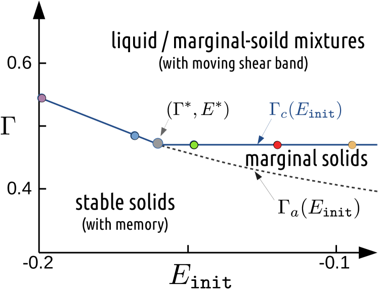
Figure 2: “Phase diagram” classifying driving conditions ($E_{\text{init}}$,$\Gamma$) according to the steady-state they will reach: stable solids (strongly reminiscent of the initial state), marginal solids (shear-annealed solids independent of the initial condition), and solid-liquid mixtures characterized by an erratic shear-band. Color circles indicate $\Gamma_{c}$ for different initial degrees of annealing $E_{\text{init}}$.

As summarized in a diagram Fig.2, $\Gamma_{a}(E_{\text{init}})$ (dashed line) identifies with $\Gamma_{c}(E_{\text{init}})$ (solid line) below $E^{*}$, and bifurcates above it. The solid steady-states resulting from driving conditions below $\Gamma_{a}(E_{\text{init}})$ are strongly reminiscent of the initial state and called “stable solids”. In contrast, those driving conditions in between $\Gamma_{c}$ and $\Gamma_{a}$ correspond to solids that forget their initial condition and end up being “marginal solids” in the steady-state. Driving conditions in the region above $\Gamma_{c}(E_{\text{init}})$ lead to a steady-state mixed phase composed by a fluid shear band surrounded by a critical marginal solid, which we detail in the following.

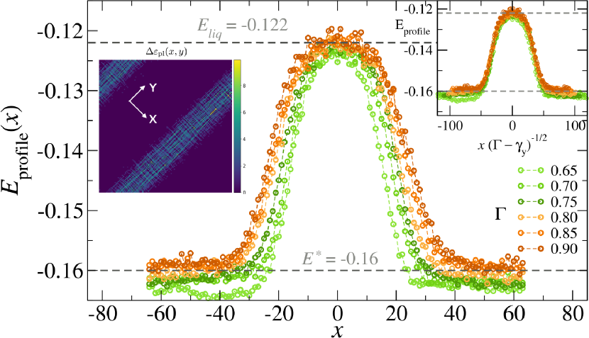
Figure 3: Energy profiles averaged along the y-axis for different $\Gamma$. $x=0$ is set to the maximum location. Left inset: map of strain field during a half-cycle in the steady-state. Right inset: profiles collapse using $w_{s}(\Gamma)=a(\Gamma-\Gamma_{0})^{\alpha}$ with $\Gamma_{0}=\gamma_{y}=0.413$ and $\alpha=1/2$.

Fig. 3 shows the averaged stress-free energy profile across a section orthogonal to the shear-band Manning, Langer, and Carlson (2007) (evidenced in the strain field in the left-inset). The energy profile characterizes the band by a bell-shape. The interior of the band (top of the bell) has the same energy as the stationary liquid in uniform shear deformation $E_{\text{liq}}\approx-0.122$. The width $w_{s}$ of the band increases with $\Gamma$ and is well fitted by $w_{s}(\Gamma)=a(\Gamma-\Gamma_{0})^{\alpha}$. A good collapse is found when rescaling the profiles with $\alpha=1/2$ (right-inset of Fig. 3), reminiscent of the transient band dynamics in uniform shearJagla (2010). We further notice two peculiarities: First, from the fit, $\Gamma_{0}$ identifies with $\gamma_{y}$ instead of $\Gamma^{*}$, implying that at the transition, the shear-band has a finite width $w_{s}(\Gamma^{*})>0$ (because $\gamma_{y}<\Gamma^{*}$). Second, the energy profile is independent on $E_{\text{init}}$ and the energy at the bottom of the bell-shape coincides with the critical solid energy $E^{*}$. This allows to conclude that the mixture phase is completely independent on the initial degree of annealing and uniquely characterized by the width $w_{s}$: the stationary regime is composed of a fraction of critical solid at energy $E^{*}$ and a shear-band made of the liquid of energy $E_{\rm liq}$. Since $E_{\text{liq}}>E^{*}$, the monotonic growth of $E_{\tt sf}^{\tt stat}$ (Fig. 1(b)) can be rationalized in terms of the shear-band widening with $\Gamma$:

$$E_{\tt sf}^{\tt stat}\simeq E^{*}+\left(E_{\rm{liq}}-E^{*}\right)\frac{a(\Gamma-\gamma_{y})^{\alpha}}{L}.$$ (1)

The validity of this behavior is tested in Fig. 1(b) (orange line). From our analysis, the transition seems to be of first order in nature for two reasons: First, the jump in $E_{\tt sf}^{\tt stat}$ is clearly discrete for well annealed samples, but it appears discontinuous also for the poorly annealed systems, where around $\Gamma^{*}$ we observe energy fluctuations between two close but distinct levels (see the inset of Fig. 1(b)): $E_{\tt sf}^{\tt stat}\approx-0.16$ for the realizations that remain in the solid phase and $E_{\tt sf}^{\tt stat}\approx-0.157$ for those that transition to the mixed phase. Second, from the finite-size analysis of $E_{\tt sf}^{\tt stat}$ showing a nice collapse of $E_{\tt sf}^{\tt stat}$ for different system sizes $L$ in Fig. 9 (Appendix.D), we can conclude that the shear band when appearing invades a finite portion of the system Parmar, Kumar, and Sastry (2019); Yeh et al. (2020); Das, Vinutha, and Sastry (2020); Bhaumik, Foffi, and Sastry (2021); Leishangthem, Parmar, and Sastry (2017) $w_{s}(\Gamma^{*})/L>0$. The first-order nature of the transition in energy $E_{\tt sf}^{\tt stat}$ at $\Gamma^{*}$ is further elaborated in Appendix.D.

III.2 Transient properties

 

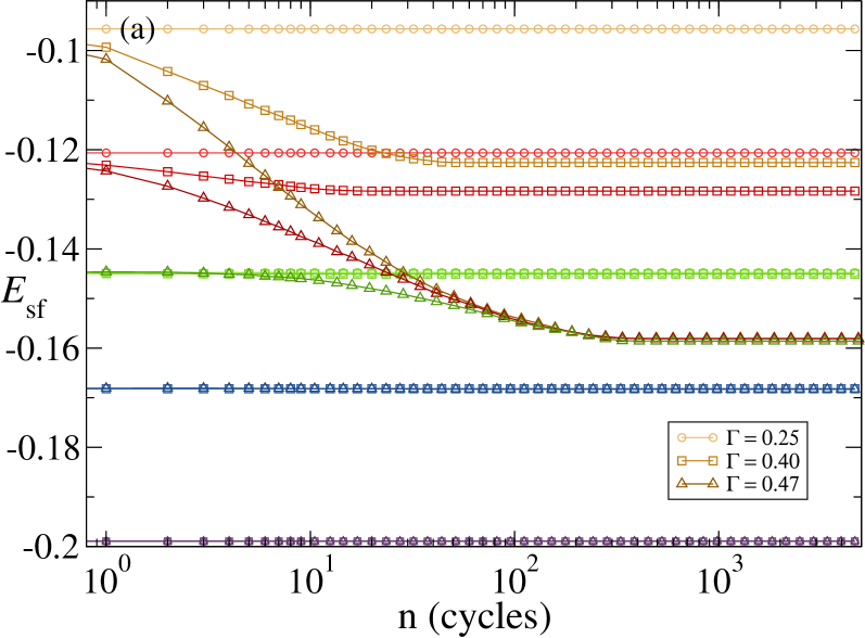
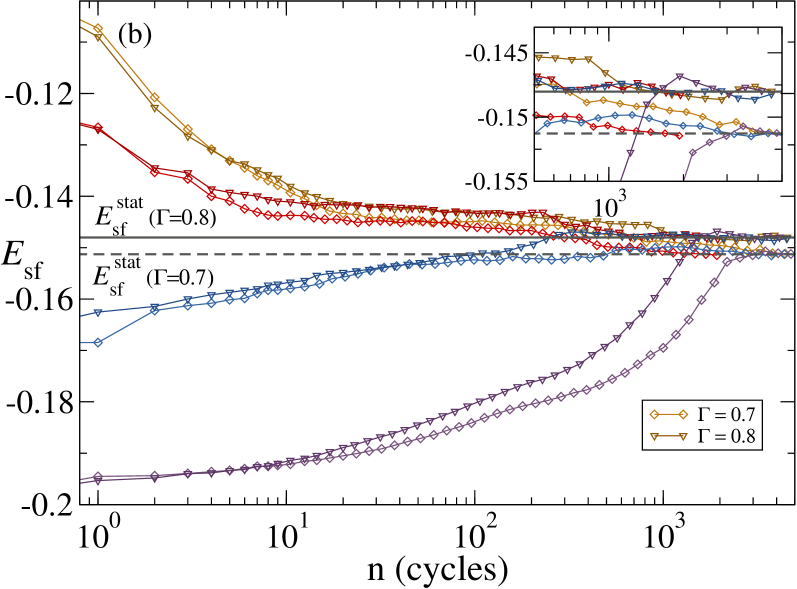
Figure 4: Transient properties– Evolution of stress-free energy $E_{\tt sf}$ as the number of cycles $n$ increases, for different amplitudes. Colors coding for different $E_{\text{init}}$ are the same as in Fig.1. System size is $128^{2}$. (a) Solid phase ($\Gamma\!<\!\Gamma_{c}$). (b) Mixed phase ($\Gamma\!>\!\Gamma_{c}$). The inset shows a zoom-in to appreciate the difference in $E_{\tt sf}^{\tt stat}$ at different $\Gamma$.

We now discuss the transient oscillatory dynamics. Fig.4 shows the evolution of $E_{\tt sf}(n)$, as the oscillation cycles $n$ accumulate, for different driving conditions $(E_{\text{init}},\Gamma)$. Below $\Gamma_{c}$ (Fig.4(a)), ultra-stable systems ($E_{\text{init}}<E^{*}$) are unperturbed by the oscillations, while systems with $E_{\text{init}}>E^{*}$ shear-anneals if the amplitude is large enough. At amplitudes above $\Gamma_{a}(E_{\text{init}})$ all initial conditions are shear-annealed to the same stationary state, as observed for our three softest samples in Fig. 4(a). Above $\Gamma_{c}$ (Fig.4(b)), all samples go to the same stationary state at large $n$. Our observations for the number $n_{T}$ of cycles to reach steady-states are compatible with a divergence when approaching $\Gamma_{c}$ reported in previous worksLeishangthem, Parmar, and Sastry (2017); Khirallah et al. (2021); Sastry (2021); Fiocco, Foffi, and Sastry (2013); Kawasaki and Berthier (2016). Data for ($\Gamma<\Gamma_{c}$) is shown in AppendixE.

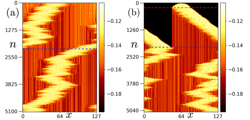
Figure 5: Energy profiles $E_{\tt profile}(x)$ evolving as function of the number $n$ of oscillation cycles for $\Gamma=0.7$. Light colors represent higher energies and evidence the position of the shear-band. (a) A poorly annealed sample with $E_{\text{init}}\approx-0.12$ (see also Video 1 (Multimedia view)). (b) Well annealed sample with $E_{\text{init}}\approx-0.199$ (see also Video 2 (Multimedia view)). The red dashed-line in (b) indicates the stabilization of the band width at $n\approx 220$. When the blue dashed-line is reached, the band has visited the entire system.

We switch now to the observation of different dynamical regimes for the mixed phase. For poorly annealed samples, the onset of the shear-band and its stabilization in a stationary width $w_{s}(\Gamma)$ occurs gradually and rapidly as the solid region shear-anneals to the critical state in a small number of cycles. Then the shear band diffuses in the material (see Fig. 5(a) and Video 1 (Multimedia view)) with a mobility that increases with $\Gamma$. In well annealed systems instead, the transient is richer and we identify three dynamical regimes (Fig. 5(b), see also Video 2 (Multimedia view)): (i) Shear band formation and growth. The initial band growth is observed at the top of Fig. 5(b) (see Fig.11 in AppendixF for a more detailed illustration for the initial band growth). This initial coarsening of the shear-band is studied in Fig. 6 at different $\Gamma$. In all cases, the band width grows as $\sim n^{1/3}$ until reaching the stationary width $w_{s}\sim(\Gamma-\gamma_{y})^{1/2}$. (ii) Melting of the solid. The now fully-formed shear band displays a ballistic motion preferentially invading the deeply annealed solid and leaving behind the critical solid of energy $E^{*}$. (iii) Shear band diffusion. When the shear-band has visited the entire system, all the regions outside the band have been modified into the critical marginal solid. The stationary state is reached and the band diffuses forever, maintaining its characteristic $\Gamma$-dependent width.

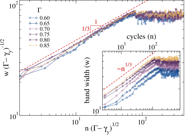
Figure 6: Shear-band width $w$ as a function of $n$ for different $\Gamma$. The initial condition is a well annealed solid ($E_{\text{init}}=-0.168$). The inset shows raw-data and the main panel the scaling $w(\Gamma-\gamma_{y})^{-1/2}$ vs. $n(\Gamma-\gamma_{y})^{1/2}$. The red dashed line is a power-law $\sim n^{1/3}$. System size is $256^{2}$.

IV Discussion

Our mesoscopic model allows to recover the phenomenology of the oscillatory shear of amorphous materials reported by MD simulationsLeishangthem, Parmar, and Sastry (2017); Bhaumik, Foffi, and Sastry (2021); Das, Vinutha, and Sastry (2020); Ozawa et al. (2018); Yeh et al. (2020); Das, Vinutha, and Sastry (2020) and go beyond. While some emerging features can be already captured by even further simplified toy models as seen recentlySastry (2021), keeping an spatial extent for the system and its geometry gives access to the full picture. We are able to univocally classify the oscillatory stationary states according to a “phase diagram” in the space of oscillation amplitude $\Gamma$ and initial annealing level $E_{\text{init}}$, and relate them with the steady-states of the uniform-deformation protocol. Interestingly, the oscillatory protocol always shows a discontinuous transition in both stress and energy at a critical strain amplitude $\Gamma_{c}$, even in the case of ductile materials that melt homogeneously under uniform deformation. Notably, ductile materials mechanically anneal and harden at sub-critical amplitudes under oscillatory shear. Independently on the initial state, every system sheared at large amplitudes ends up in a steady-state displaying a permanent shear-band. This band contains a stationary fluid identical to the one obtained at large uniform deformations and is embedded in a solid matrix which is not at all arbitrary. The solid surrounding the shear-band in this mixed phase is the critical marginal solid that has the energy of the critical annealing level $E^{*}$. A line of amnesia $\Gamma_{a}(E_{\text{init}})$ discriminate driving conditions ($E_{\text{init}}$, $\Gamma$) between stable solids and solids that shear-anneal and evolve towards a marginal line in the steady-state. Our approach gives also transparent access to the transient regimes of shear-band formation, growth and motion. For deeply-annealed samples, a small but finite width band first spreads the system, then grows with a power-law $\propto n^{1/3}$ of the number of oscillation cycles. Ulteriorly, the band invades ballistically the deeply-annealed solid, leaving behind the critical solid of energy $E^{*}$. Finally, is diffuses anomalously over all the system.

These results shed light to clarify some previous observations in the literature and open interesting directions of new research. One could ask, for example, whether the emergence of a transient state of multiple shear-bands is possible in the large system limit, and how do they merge in a single band in the steady-state (or not). Also, to which extent the incorporation of “reversible” plastic events observed in atomistic simulationsMungan et al. (2019); Kawasaki and Berthier (2016); Regev, Lookman, and Reichhardt (2013); Regev et al. (2015); Priezjev (2016); Regev and Lookman (2018); Fiocco, Foffi, and Sastry (2013) enriches the overall phenomenology. Those are absent in our present model by choice, but easy to include by locally quenching the disordered potential Khirallah et al. (2021). Further, the critical annealing $E^{*}$ detected in the oscillatory protocol could play also a relevant role in uniform shear, where the ductile-brittle yielding transition is a matter of vivid discussionOzawa et al. (2018, 2018); Fielding (2021); Barlow, Cochran, and Fielding (2020). It is indeed suggestive that the load curve of our closest to $E^{*}$ sample sits near to the apparent transition between ductile/brittle yielding probed by the uniform shear curves. More importantly, it will be interesting to test experimentally these predictions, with new measurements closer to the quasi-static limit, since in the standard setups the oscillations are relatively fast and the material softens instead of annealing and hardening.

Moreover, general features of our phase diagram could find analogies in different systems with elastic interactions, irreversible events and quenched disorder, such as vortex or skyrmion systems where the initial state can be also prepared in different ways Mangan, Reichhardt, and Reichhardt (2008); Okuma, Tsugawa, and Motohashi (2011); Brown, Reichhardt, and Reichhardt (2019); Maegochi, Ienaga, and Okuma (2021). In general, we hope that our results will motivate new research directions in the study of low temperature amorphous materials, from realistic large-scale atomistic simulations to experiments.

Appendix A Methods: Our Model

We focus on two dimensional systems. Our goal is to provide a description of the physics of amorphous materials under deformation and we use a model based on the evolution of the three strain field components Jagla (2007); Cao et al. (2018): the isotropic compression $\varepsilon_{1}(\mathbf{r})$ and the shear components $\varepsilon_{2}(\mathbf{r})$ and $\varepsilon_{3}(\mathbf{r})$. The latter are bi-axial deformations (compression along some direction, expansion perpendicularly), the difference between $\varepsilon_{2}(\mathbf{r})$ and $\varepsilon_{3}(\mathbf{r})$ is that the compression/expansion axis are the $x-y$ axis for the first, and the lines at $45$ degrees for the second (Recall that given the continuum displacement field, $\mathbf{u(r)}=\left(u_{1}(\mathbf{r}),u_{2}(\mathbf{r})\right)$, the elements of strain tensor are given by $\epsilon_{ij}(\mathbf{r})=\frac{1}{2}(\partial_{i}u_{j}(\mathbf{r})+\partial_{j}u_{i}(\mathbf{r}))$. Then $\varepsilon_{1}(\mathbf{r})=\left(\epsilon_{11}(\mathbf{r})+\epsilon_{22}(\mathbf{r})\right)/2$, $\varepsilon_{2}(\mathbf{r})=\left(\epsilon_{11}(\mathbf{r})-\epsilon_{22}(\mathbf{r})\right)/2$ and $\varepsilon_{3}(\mathbf{r})=\epsilon_{12}(\mathbf{r})$). For a perfectly elastic solid, one can write the energy of any deformation in terms of a quadratic elastic functional

$$E_{\text{elast.}}=\int d^{2}\mathbf{r}\,\left(B\varepsilon_{1}^{2}+\mu\varepsilon_{2}^{2}+\mu\varepsilon_{3}^{2}\right)\,,$$ (2)

where $B$ and $\mu$ are respectively the bulk and shear modulus. Here we use $B=1$ and $\mu=1/2$. This purely elastic functional has a single minimum, which corresponds to the undeformed state. When a deformation is applied, it brings the system out of such a minimum; when released, a restoring stress brings the system back to its undeformed state. If we want to take plasticity into account, irreversible deformations should be allowed; for example, the energy landscape may be characterized by multiple local minima separated by finite barriers (similar to the case of sheared vortices in random quenched potentials Maegochi, Ienaga, and Okuma (2021); Okuma, Tsugawa, and Motohashi (2011)). Here, we study the response of the material under simple shear. We account for the plastic events by replacing the harmonic term $\mu\varepsilon_{3}^{2}$ in Eq. 2 with a disordered potential $V_{\underline{x}}[\mathbf{r},\varepsilon_{3}]$ that displays many minima as $\varepsilon_{3}$ varies. The other two strain components, $\varepsilon_{1}$ and $\varepsilon_{2}$, are expected to remain small, and the quadratic approximation, to hold. The energy functional then becomes

$$E_{plast.}=\int d^{2}\mathbf{r}\,\left(B\varepsilon_{1}^{2}+\mu\varepsilon_{2}^{2}+V_{\underline{x}}[\mathbf{r},\varepsilon_{3}]\right)\;$$ (3)

The subscript of $V_{\underline{x}}$ represents an internal degree of freedom. Thus the disorder potential is not a function of the strain field $\varepsilon_{3}(\mathbf{r})$ only. The origin of that internal degree of freedom is justified as follows: In amorphous materials, the disorder is not generated by immobile impurities but rather by the random-like configurations of the particles position $\underline{x}$. Plastic events, called shear transformations, are localized in space. When an event occurs in the region $\mathbf{r}$, the particles inside the region rearrange irreversibly from $\underline{x}$ to $\underline{x}^{\prime}$. This rearrangement is mimicked in the model by two features.

• First, $\varepsilon_{3}(\mathbf{r})$ overcomes a local energetic barrier and reach the basin of a new minimum of the disordered potential.

• Second, the basin of the old minimum also modifies irreversibly as new configuration of particles positions imposes a new disorder potential.

In the spirit of keeping only the essence of the physical process involving local plastic events, we model the disorder of each region $\bm{r}$ as a collection of pieces of harmonic potential:

$$V_{\text{parab}}(\varepsilon_{3})=\mu[(\varepsilon_{3}-\epsilon_{pl})^{2}-\epsilon_{w}^{2}],\quad\text{for}\,|\varepsilon_{3}-\epsilon_{pl}|<\epsilon_{w}.$$ (4)

The random parameters $\epsilon_{pl}$ and $\epsilon_{w}$ vary from region to region: $\epsilon_{pl}$ defines the location of the minimum and $\epsilon_{w}$, the semi-width of the potential. Once the strain $\varepsilon_{3}$ overcomes the barriers of the parabolic basin a new semi-width $\epsilon_{w}^{\prime}$ is drawn from a triangular distribution of mean $1/2$ and standard-deviation $1/20$. The new minimum of the potential is updated as follows:

• When $\varepsilon_{3}$ overcomes the barrier at $\epsilon_{pl}-\epsilon_{w}$ then the new minimum is located at $\epsilon_{pl}-(\epsilon_{w}+\epsilon_{w}^{\prime})$

• When $\varepsilon_{3}$ overcomes the barrier at $\epsilon_{pl}+\epsilon_{w}$ then the new minimum is located at $\epsilon_{pl}+(\epsilon_{w}+\epsilon_{w}^{\prime})$.

It is important to stress that once strain $\varepsilon_{3}$ overcomes the barriers of the parabolic basin the local basin changes irreversibly, even is the $\varepsilon_{3}$ moves backward.

The three components of the strain field are not independent but obey the St. Venant constraint Jagla (2007). As a consequence, the deformation of the material can be described by the evolution of a single component. In particular assuming, in the framework of an overdamped dynamics, that $\varepsilon_{1}$ and $\varepsilon_{2}$ relax much faster than $\varepsilon_{3}$, we arrive to

$$\partial_{t}\varepsilon(\mathbf{r},t)=\int d^{2}\mathbf{r}^{\prime}G(\mathbf{r-r^{\prime}})\varepsilon(\mathbf{r}^{\prime})+\eta_{{}_{\underline{x}}}(\mathbf{r},\varepsilon)+\Sigma_{\text{ext}}.$$ (5)

Here, $\varepsilon(\mathbf{r},t)$ has replaced $\varepsilon_{3}(\mathbf{r},t)$ for a lighter notation and the kernel $G(\mathbf{r})$ is the long-range Eshelby’s propagator. For simple shear, using the method in Cao et al. (2018), the propagator can be written in terms of the polar coordinates $\mathbf{r}=(r,\theta_{\mathbf{r}})$ as

$$G(\mathbf{r})=\frac{2\sqrt{2}B}{\pi r^{2}}\frac{3\cos(4\theta_{\mathbf{r}})-1}{\left(3-\cos(4\theta_{\mathbf{r}})\right)^{2}}\,.$$ (6)

Finally, $\eta_{{}_{\underline{x}}}$ is originated from the disorder potential as $-\partial_{\varepsilon}V_{{}_{\underline{x}}}$ and $\Sigma_{\text{ext}}$ is the external applied stress.

For our purposes, it is important to control the macroscopic strain instead of the macroscopic stress. In order to achieve this, one can replace $\Sigma_{\text{ext}}$ with $\kappa(\gamma-\overline{\varepsilon})$ in Eq.5 ($\overline{\varepsilon}$ indicates the macroscopic strain defined as the spatial average of $\varepsilon(\mathbf{r})$). For large values of $\kappa$, it is expected that the macroscopic strain $\overline{\varepsilon}$ is close to $\gamma$. The slope of the stress-strain curve is given by $\mathcal{G}=2\kappa\mu/(\kappa+2\mu)$. Here we use $\kappa=10$ and $\mu=1/2$, so we get $10/11\approx 0.91$ used as the initial slope of the stress-strain curve in the main text.

The energy functional defined in Eq.3 can be equivalently written as

$$E_{\text{plast.}}[\varepsilon(\bm{r})] = \int d^{2}\bm{r}e(\bm{r})$$

$$\text{with}\quad e(\bm{r}) \hat{=} \frac{1}{2}\varepsilon(\bm{r})\int d\bm{r}^{\prime}G(\bm{r}-\bm{r}^{\prime})\varepsilon(\bm{r}^{\prime})$$ (7)

$$+ V_{\underline{x}}\left(\bm{r},\varepsilon(\bm{r})\right).$$

Thus our system can be viewed as an elastic manifold $\varepsilon(\bm{r})$ (with long-range interactions among all sites) living in an energy landscape where each site has its independent disordered potential. The stress-free energy used in the main text is then defined as the plastic energy per site: $E_{\tt sf}\hat{=}E_{\text{plast.}}[\varepsilon*]/L^{2}$, with $\frac{\delta E_{\text{plast.}}}{\delta\varepsilon(\bm{r})}\big{|}_{\varepsilon^{*}}=0$. The energy profiles of the main text are obtained by averaging the local energy to $e(\bm{r})$ along the direction of the shear band. We apply quasi-static deformation $\gamma$ by numerically solving Eq.5 mapped onto a lattice system.

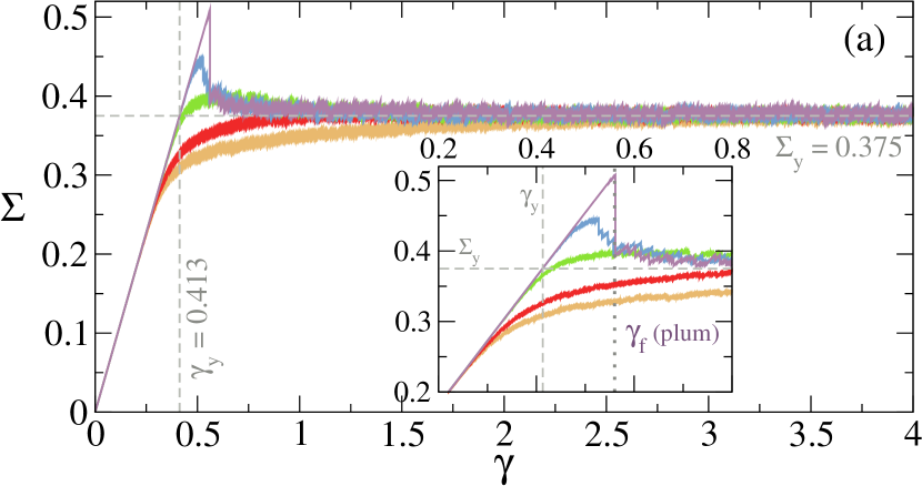
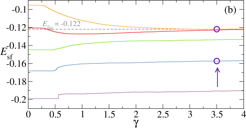
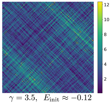
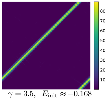
Figure 7: Uniform shear deformation for different degrees of initial annealing ($E_{\text{init}}\approx$ -0.095 (chocolate), -0.12(red), -0.149(chamelon), -0.168(blue), -0.199(plum)). (a) Stress-strain curves for different initial degrees of annealing. The yield stress $\Sigma_{y}=0.375$ defined as the plateau is also indicated. (b) Evolution of the stress-free energy $E_{\tt sf}=E(\Sigma)-\Sigma^{2}/(4\mu)$ during the deformation. The stationary plateau $E_{\text{liq}}=-0.122$ is also indicated. (c): Colormap of the local deformation field at $\gamma=3.5$ for two samples prepared at different degrees of annealing, circles in (b).

Special care is taken for the initial condition, since we want to mimic different degrees of annealing in our samples. In our model, a well-annealed sample corresponds to an initial condition where the local strains are confined in deep potential wells, while poorly-annealed samples correspond to a strain manifold confined in shallow potential wells. In practice we start from a liquid configuration of local energy basins obtained after a long uniform shear. Then, to prepare samples of different degree of annealing we change the depths of the parabolic wells, $\epsilon_{w}$. To obtain deeply annealed samples we also align the centers, $\epsilon_{pl}$, to their mean value. Finally, we let the local strain relax to its stress-free configuration, and that makes our initial condition to start the oscillatory deformation. We performed simulations for systems of sizes $N=32\times 32,64\times 64,128\times 128,256\times 256$. The data shown in this work correspond to the two largest systems.

Appendix B Uniform shear deformation curves

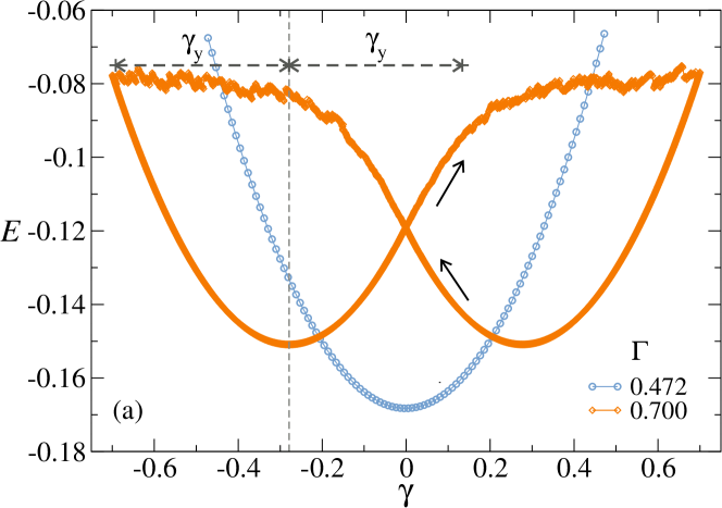
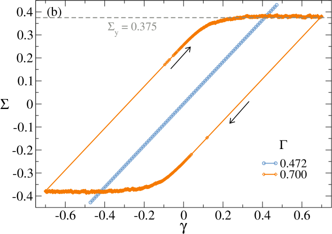
Figure 8: (a) Energy versus strain in the oscillatory steady state (only one loop shown) for $\Gamma=0.45$ (light-blue circles) and $\Gamma=0.7$ (orange diamonds). The little black arrows mark the sense of the loop. (b) Stress as a function of strain in the oscillatory steady state for the same two amplitudes as above.

We present in this section more detailed results for the case of uniform shear deformation. In Fig.7(a), we show the same stress-strain curves as Fig.1a of the main text with a larger scope of strain up to $\gamma=4$, so that the common plateau $\Sigma_{y}\approx 0.375(\pm 0.003)$ at long strains is well captured. We show system’s stress-free energy as function of strain in Fig.7(b). Poorly annealed samples (those which do not display a failure) reach rather quickly a common energy plateau $E_{\text{liq}}\approx-0.122(\pm 0.001)$ which corresponds to the fully formed stationary liquid state. In contrast, well annealed samples display different and slowly-evolving transient regimes. These differences can be understood as follows: Poorly annealed systems melt at deformations around $\gamma_{y}$ into a non-Newtonian liquid which has no memory of the initial degree of annealing (see Fig.7 bottom-left). In well annealed systems, instead, the non-Newtonian liquid is localised within a shear band and the solid part is unchanged, insensitive to the deformation (see Fig.7 bottom-right). When $\gamma$ is increased further, the band widens. As discussed in Jagla (2010), we expect $w(\gamma)\propto\sqrt{\gamma-\gamma_{\tt f}}$. Eventually, for very large $\gamma$, the band width reaches the system size and the whole sample lose memory of the initial condition converging to the stationary value $E_{\text{liq}}$.

Appendix C Typical loops in oscillatory stationary states

In Fig. 8, we show the total energy $E$ (per volume) as a function of $\gamma$ during a steady oscillation between $\pm\Gamma$. While in the solid phase ($\Gamma<\Gamma_{c}$), the energy displays a single parabolic shape, corresponding to an elastic behavior, in the mixed phase ($\Gamma>\Gamma_{c}$), the energy has a butterfly shape: two shifted parabola are followed by a noisy plateau which reveals the presence of the liquid state. The two parabolas have an extension of $\gamma_{y}$ at both sides and the maximal stress, at $\pm\Gamma$, saturates to $\Sigma_{y}$, which also supports that the shear band is made of the stationary liquid state at large uniform shear, where plasticity dominates the dynamics once sheared beyond $\gamma_{y}$ from a zero stress state.

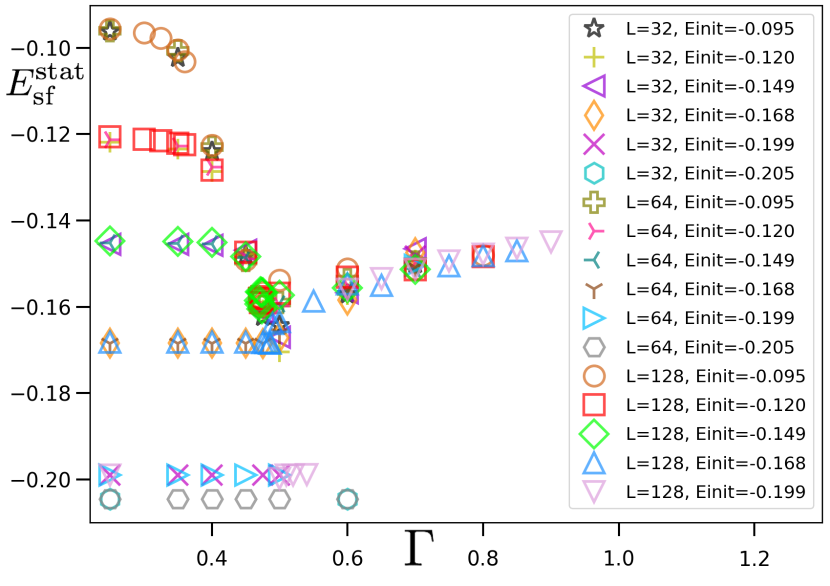
Figure 9: $E_{\tt sf}^{\tt stat}$ versus $\Gamma$ for all system sizes and initial conditions $E_{\text{init}}$ as indicated in the figure.

Appendix D The discontinuous transition in $E_{\tt sf}^{\tt stat}$ across $\Gamma^{*}$

In Fig.9 we observe that, at different amplitudes $\Gamma$, $E_{\tt sf}^{\tt stat}$ (namely the steady-state stress-free energies per unit volume) does not depend on the system size. As a consequence, in the mixed phase, for $\Gamma>\Gamma_{c}\geq\Gamma^{*}$, the shear band invades a finite fraction $r=w_{s}/L$ of the system, with $w_{s}$ representing the width of shear band. We can evaluate this fraction by observing that, in the stationary state, during the oscillation driving from $-\Gamma$ to $\Gamma$, the material behaves initially as a solid and accumulates an elastic strain $\approx 2\gamma_{y}$ (see e.g. Fig.8), the rest of the macroscopic deformation $2\Gamma-2\gamma_{y}$ consists of the plasticity confined within the shear band, denoted $\gamma_{\text{plt}}$. Formally, one may write:

$$2\Gamma-2\gamma_{y}=r\gamma_{\text{plt}}\;.$$ (8)

Since plasticity takes place significantly only during the loading from $-\Gamma+2\gamma_{y}$ to $+\Gamma$, it is reasonable to assume

$$\gamma_{\text{plt}}\propto(2\Gamma-2\gamma_{y})^{x}\;,\quad\text{with}\quad x>0.$$ (9)

Combining the two relations takes to

$$r(\Gamma) = K(\Gamma-\gamma_{y})^{1-x}\;,$$

$$w_{s}(\Gamma) = r\cdot L=a(\Gamma-\gamma_{y})^{1-x}\;.$$ (10)

with $K>0$ a constant independent on the system size. A simple guess, by taking arguments from ref. Jagla (2010), is $x\approx 1/2$, and this yields our empirically observed $\alpha\approx 1/2$, while identifying $\Gamma_{0}$ with $\gamma_{y}$ (Fig.3)

Now two scenarios are possible: (i) if $\gamma_{y}=\Gamma^{*}$, the transition is of second order in nature as the fraction of liquid material vanishes at the transition. (ii) If $\gamma_{y}<\Gamma^{*}$, the transition is of first order in nature as the fraction of liquid material (shear band) is finite at the transition $\Gamma^{*}$. We can argue that the second scenario is correct. Indeed $\gamma_{y}$ is the elastic strain beyond which a liquid-state material (of $E_{\text{liq}}$) melts and its stress-strain curve bends Bonn et al. (2017). By our model construction, we have $|E_{\text{liq}}|\propto\gamma_{y}^{2}$. On the other hand, for a critical marginal solid, we have $|E^{*}|\propto{\Gamma^{*}}^{2}$ by its definition. Thus, we have $\Gamma^{*}\propto\sqrt{|E^{*}|}>\sqrt{|E_{\text{liq}}|}\propto\gamma_{y}$.

Combining the above arguments and our empirical data analysis, we can conclude for the stress-free energy of poorly annealed samples that $E_{\text{sf}}^{\text{stat}}(\Gamma^{*-})=E^{*}<E^{*}+K(E_{\text{liq}}-E^{*})(\Gamma^{*}-\gamma_{y})^{\alpha}=E_{\text{sf}}^{\text{stat}}(\Gamma^{*+})$, i.e. a discontinuity across $\Gamma^{*}$, with the predicted jump ($\sim 0.0045$) appearing consistent with the fluctuation amplitude in the inset of Fig.1(b).

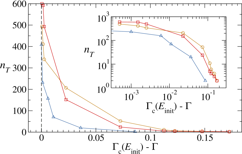
Figure 10: Number of cycles needed to reach the steady state as a function of the distance to the critical amplitude, for different initial annealing levels $E_{\text{init}}$.

Appendix E Duration of the oscillatory transient regime

The number of cycles needed to reach the stationary state is an observable that that is expected to diverge at the transition, as seen equally in molecular dynamics of sheared amorphous solids Khirallah et al. (2021); Sastry (2021) and in models of sheared vortices in disordered media Okuma, Tsugawa, and Motohashi (2011); Brown, Reichhardt, and Reichhardt (2019). We show in Fig.10 the number $n_{T}$ of oscillation cycles needed to reach the stationary state in our system for $\Gamma<\Gamma_{c}$ and $E_{\text{init}}>E^{*}$. $n_{T}$ is easily measured in such situations since the stationary state is unambiguously identified once a perfect periodic loop of stress/energy (e.g. the blue curves in Fig.8) is established. Instead of a power-law divergence Khirallah et al. (2021); Sastry (2021), we observe rather $n_{T}\propto\log\left(\frac{1}{\Gamma_{c}-\Gamma}\right)$. The stationary state of well annealed systems $E_{\text{init}}<E^{*}$ oscillated at $\Gamma<\Gamma_{c}(E_{\text{init}})$ is strongly reminiscent of its initial condition, as mentioned in the main text, and thus reached almost immediately. Only at $\Gamma$ very close to $\Gamma_{c}$, a slight increase of $n_{T}$ is observed due to increased local adjustment, the nature of which is an open question. Above $\Gamma_{c}$, when $\Gamma$ is approaching $\Gamma_{c}$, the system suffer a drastic dynamic slowing down that makes an accurate measurement of $n_{T}$ more difficult. A more careful assessment of the specific law displayed by our model for the divergence of $n_{T}$ at $\Gamma_{c}$ is left for future investigation.

Appendix F Shear-band emergence in well annealed samples

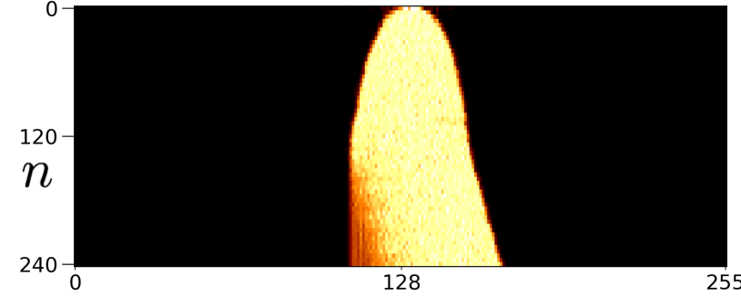
Figure 11: The energy profile across a section perpendicular to the shear band evolving as function of the number $n$ of oscillation cycles. The light color region represents the position of the shear band with a higher energy. The amplitude of the oscillation is $\Gamma=0.7$. The sample, of linear size $L=256$, has initially been prepared at $E_{\text{init}}\approx-0.199$, i.e., in a very well annealed state.

In Fig.11 we show a color-map image similar to Fig. 4 of the main text. It depicts the energy profile evolution as function of the number of oscillation cycles $n$ in the first stages of the transient dynamics of an initially well annealed sample (here a sample of system size $L=256$ for a better visualisation). The inverted parabolic-like shape observed as $n$ increases illustrates the band coarsening. In fact the bad-width growth law is rather $w\sim n^{1/3}$. At about $n\sim 120$ steps, the band has reached a stable width and starts moving ballistically to the right, leaving behind a marginal solid.

References

- Bonn et al. (2017) D. Bonn, M. M. Denn, L. Berthier, T. Divoux, and S. Manneville, “Yield stress materials in soft condensed matter,” Rev. Mod. Phys. 89, 035005 (2017).
- Nicolas et al. (8 12) A. Nicolas, E. E. Ferrero, K. Martens, and J.-L. Barrat, “Deformation and flow of amorphous solids: Insights from elastoplastic models,” Rev. Mod. Phys. 90, 045006 (2018-12).
- Shi and Falk (2006) Y. Shi and M. L. Falk, “Atomic-scale simulations of strain localization in three-dimensional model amorphous solids,” Phys. Rev. B 73, 214201 (2006).
- Ozawa et al. (2018) M. Ozawa, L. Berthier, G. Biroli, A. Rosso, and G. Tarjus, “Random critical point separates brittle and ductile yielding transitions in amorphous materials,” Proceedings of the National Academy of Sciences 115, 6656–6661 (2018).
- Popović, de Geus, and Wyart (2018) M. Popović, T. W. J. de Geus, and M. Wyart, “Elastoplastic description of sudden failure in athermal amorphous materials during quasistatic loading,” Phys. Rev. E 98, 040901 (2018).
- Barlow, Cochran, and Fielding (2020) H. J. Barlow, J. O. Cochran, and S. M. Fielding, “Ductile and brittle yielding in thermal and athermal amorphous materials,” Phys. Rev. Lett. 125, 168003 (2020).
- Ozawa et al. (2021) M. Ozawa, L. Berthier, G. Biroli, and G. Tarjus, “Rare events and disorder control the brittle yielding of amorphous solids,” (2021), arXiv:2102.05846 [cond-mat.soft] .
- Richard, Rainone, and Lerner (2021) D. Richard, C. Rainone, and E. Lerner, “Finite-size study of the athermal quasistatic yielding transition in structural glasses,” The Journal of Chemical Physics 155, 056101 (2021).
- Fielding (2021) S. M. Fielding, “Yielding, shear banding and brittle failure of amorphous materials,” arXiv preprint arXiv:2103.06782 (2021).
- Fiocco, Foffi, and Sastry (2014) D. Fiocco, G. Foffi, and S. Sastry, “Encoding of memory in sheared amorphous solids,” Phys. Rev. Lett. 112, 025702 (2014).
- Leishangthem, Parmar, and Sastry (2017) P. Leishangthem, A. D. S. Parmar, and S. Sastry, “The yielding transition in amorphous solids under oscillatory shear deformation,” Nature Communications 8, 14653 EP – (2017).
- Das, Parmar, and Sastry (2020) P. Das, A. D. S. Parmar, and S. Sastry, “Annealing glasses by cyclic shear deformation,” (2020), arXiv:1805.12476 [cond-mat.soft] .
- Hexner, Liu, and Nagel (2020) D. Hexner, A. J. Liu, and S. R. Nagel, “Periodic training of creeping solids,” Proceedings of the National Academy of Sciences 117, 31690–31695 (2020).
- Sastry (2021) S. Sastry, “Models for the yielding behavior of amorphous solids,” Phys. Rev. Lett. 126, 255501 (2021).
- Khirallah et al. (2021) K. Khirallah, B. Tyukodi, D. Vandembroucq, and C. E. Maloney, “Yielding in an integer automaton model for amorphous solids under cyclic shear,” Phys. Rev. Lett. 126, 218005 (2021).
- Yeh et al. (2020) W.-T. Yeh, M. Ozawa, K. Miyazaki, T. Kawasaki, and L. Berthier, “Glass stability changes the nature of yielding under oscillatory shear,” Phys. Rev. Lett. 124, 225502 (2020).
- Kawasaki and Berthier (2016) T. Kawasaki and L. Berthier, “Macroscopic yielding in jammed solids is accompanied by a nonequilibrium first-order transition in particle trajectories,” Physical Review E 94, 022615 (2016).
- Regev, Lookman, and Reichhardt (2013) I. Regev, T. Lookman, and C. Reichhardt, “Onset of irreversibility and chaos in amorphous solids under periodic shear,” Phys. Rev. E 88, 062401 (2013).
- Regev et al. (2015) I. Regev, J. Weber, C. Reichhardt, K. A. Dahmen, and T. Lookman, “Reversibility and criticality in amorphous solids,” Nature Communications 6, 8805 EP – (2015).
- Fiocco, Foffi, and Sastry (2013) D. Fiocco, G. Foffi, and S. Sastry, “Oscillatory athermal quasistatic deformation of a model glass,” Phys. Rev. E 88, 020301 (2013).
- Priezjev (2016) N. V. Priezjev, “Reversible plastic events during oscillatory deformation of amorphous solids,” Phys. Rev. E 93, 013001 (2016).
- Priezjev (2017) N. V. Priezjev, “Collective nonaffine displacements in amorphous materials during large-amplitude oscillatory shear,” Phys. Rev. E 95, 023002 (2017).
- Regev and Lookman (2017) I. Regev and T. Lookman, “The irreversibility transition in amorphous solids under periodic shear,” in Avalanches in Functional Materials and Geophysics (Springer, 2017) pp. 227–259.
- Regev and Lookman (2018) I. Regev and T. Lookman, “Critical diffusivity in the reversibility–irreversibility transition of amorphous solids under oscillatory shear,” Journal of Physics: Condensed Matter 31, 045101 (2018).
- Mungan et al. (2019) M. Mungan, S. Sastry, K. Dahmen, and I. Regev, “Networks and hierarchies: How amorphous materials learn to remember,” Phys. Rev. Lett. 123, 178002 (2019).
- Bhaumik, Foffi, and Sastry (2021) H. Bhaumik, G. Foffi, and S. Sastry, “The role of annealing in determining the yielding behavior of glasses under cyclic shear deformation,” Proceedings of the National Academy of Sciences 118 (2021), 10.1073/pnas.2100227118.
- Parmar, Kumar, and Sastry (2019) A. D. S. Parmar, S. Kumar, and S. Sastry, “Strain localization above the yielding point in cyclically deformed glasses,” Phys. Rev. X 9, 021018 (2019).
- Das, Vinutha, and Sastry (2020) P. Das, H. Vinutha, and S. Sastry, “Unified phase diagram of reversible–irreversible, jamming, and yielding transitions in cyclically sheared soft-sphere packings,” Proceedings of the National Academy of Sciences 117, 10203–10209 (2020).
- Jagla (2007) E. A. Jagla, “Strain localization driven by structural relaxation in sheared amorphous solids,” Phys. Rev. E 76, 046119 (2007).
- Fernández Aguirre and Jagla (8 07) I. Fernández Aguirre and E. A. Jagla, “Critical exponents of the yielding transition of amorphous solids,” Phys. Rev. E 98, 013002 (2018-07).
- Ferrero and Jagla (9 11) E. E. Ferrero and E. A. Jagla, “Elastic interfaces on disordered substrates: From mean-field depinning to yielding,” Phys. Rev. Lett. 123, 218002 (2019-11).
- Jagla (2020) E. A. Jagla, “Tensorial description of the plasticity of amorphous composites,” Phys. Rev. E 101, 043004 (2020).
- Ferrero and Jagla (2021) E. E. Ferrero and E. A. Jagla, “Properties of the density of shear transformations in driven amorphous solids,” Journal of Physics: Condensed Matter 33, 124001 (2021).
- Lin et al. (2014) J. Lin, E. Lerner, A. Rosso, and M. Wyart, “Scaling description of the yielding transition in soft amorphous solids at zero temperature,” Proceedings of the National Academy of Sciences 111, 14382–14387 (2014).
- Eshelby (1957) J. Eshelby, “The Determination of the Elastic Field of an Ellipsoidal Inclusion, and Related Problems,” Proceedings of the Royal Society A: Mathematical, Physical and Engineering Sciences 241, 376–396 (1957).
- Manning, Langer, and Carlson (2007) M. L. Manning, J. S. Langer, and J. M. Carlson, “Strain localization in a shear transformation zone model for amorphous solids,” Phys. Rev. E 76, 056106 (2007).
- Jagla (2010) E. Jagla, “Shear band dynamics from a mesoscopic modeling of plasticity,” Journal of Statistical Mechanics: Theory and Experiment 2010, P12025 (2010).
- (38) See Supplemental Material at [URL will be inserted by publisher], which also includes references…
- Mangan, Reichhardt, and Reichhardt (2008) N. Mangan, C. Reichhardt, and C. J. O. Reichhardt, “Reversible to irreversible flow transition in periodically driven vortices,” Phys. Rev. Lett. 100, 187002 (2008).
- Okuma, Tsugawa, and Motohashi (2011) S. Okuma, Y. Tsugawa, and A. Motohashi, “Transition from reversible to irreversible flow: Absorbing and depinning transitions in a sheared-vortex system,” Phys. Rev. B 83, 012503 (2011).
- Brown, Reichhardt, and Reichhardt (2019) B. L. Brown, C. Reichhardt, and C. J. O. Reichhardt, “Reversible to irreversible transitions in periodically driven skyrmion systems,” New Journal of Physics 21, 013001 (2019).
- Maegochi, Ienaga, and Okuma (2021) S. Maegochi, K. Ienaga, and S. Okuma, “Critical behavior of density-driven and shear-driven reversible–irreversible transitions in cyclically sheared vortices,” Scientific Reports 11, 1–9 (2021).
- Cao et al. (2018) X. Cao, A. Nicolas, D. Trimcev, and A. Rosso, “Soft modes and strain redistribution in continuous models of amorphous plasticity: the eshelby paradigm, and beyond?” Soft Matter 14, 3640–3651 (2018).