Single Production of Vectorlike Y Quarks at the HL-LHC

Abstract

We study single production of exotic vectorlike $Y$ quark with electric charge $|Q_{Y}|=4/3$ and its subsequent decay at the High Luminosity LHC (HL-LHC). Most of the vector like quark (VLQ) decays have the electroweak $W$ bosons in the intermediate state. Besides their direct productions singly or pairs, the $W$-bosons are involved in decay chains as a result of the decay of a top quark which contributes to the background. This is particularly the case since vectorlike $Y$ quark, which is estimated to be produced with a high cross-section, can only decay via a $W$ boson and a down type quark ($d,s,b$). We calculate the cross sections of signal (for different couplings and mass values) and relevant Standard Model (SM) backgrounds. After a fast simulation of signal and background events, estimations of the sensitivity to the parameters (mass range 1000-2500 GeV for coupling value $\kappa_{Y}=0.5$, and mass range 500-2000 GeV for coupling values $\kappa_{Y}=0.3$ and $\kappa_{Y}=0.15$) have been presented at the HL-LHC with center of mass energy $\sqrt{s}=14$ TeV and integrated luminosity projections of 300 fb^-1, 1000 fb^-1 and 3000 fb^-1.

I Introduction

The results from the experiments at the Large Hadron Collider (LHC) have confirmed the validity of the Standard Model (SM) of particle physics up to a high energy scale and intensity. The upgrade of the LHC to the high luminosity phase (HL-LHC) (key-1, ) at center-of-mass energy of 14 TeV and integrated luminosity of 3000 fb^-1 will extend the sensitivity and perspectives, with the upgraded detectors and large data, to possible opportunities beyond the SM. This upgrade will be crucial for precision measurements in the Higgs sector and for increasing the new physics discovery potential at the energy and luminosity frontier. The large data will be collected in two steps. During the first upgrade phase (Run-3), experiments are expected to collect an integrated luminosity of 300 fb^-1, whereas in the next phase (Run-4), a total amount of data corresponding to 3000 fb^-1 is foreseen.

Predictions for the existence of new fermionic resonances referred to as vectorlike quarks, which are also common in some beyond the Standard Model (BSM) scenarios, have been expressed recently. Vectorlike quarks (key-2, ; key-3, ) are defined as colour-triplet under $SU(3)$ and spin-1/2 fermions whose left-handed and right-handed chiral components have the same transformation properties under the $SU(2)\times U(1)$ gauge group.

The ATLAS (key-4, ) and CMS (key-5, ) Collaborations have published searches for single production of vectorlike $T/Y$ quarks in decay channel $T/Y\to Wb$ and set $95\%$ confidence level (C.L.) lower limits on $T$/$Y$ quark masses. The upper limits on the couplings are $|\sin\theta_{L}|=0.18$ for a singlet $T$ quark, and $|\sin\theta_{R}|=0.17$ for a $(B,Y)$ doublet model, and $|\sin\theta_{L}|=0.16$ for a $(T,B,Y)$ triplet model for a $Y$ quark mass of $800$ GeV. Within the $(B,Y)$ doublet model, the limits on the mixing parameter is comparable with the exclusion limits from electroweak precision observables in the mass range [$900-1250$] GeV (key-4, ). Upper limits are placed on the production cross section of heavy exotic quarks by the CMS experiment (key-5, ), for $Y$ quarks with coupling of $0.5$ and $B(Y\to bW)=100\%,$ the observed (expected) lower mass limits are given as $1400$ ($1000$) GeV.

Potential of the HL-LHC in searching for the bounds on mass and coupling would be higher. In the analysis, we investigate a resonance particle as vectorlike $Y$ quark in the invariant mass distributions. In order to measure its charge, leptonic decay of $W$ boson and the charge of $b$-tagged jet can be used. The single production of vector like quarks is model dependent, the framework of the model suggests vectorlike $Y(-4/3)$ quark to $Wb$ channel with a branching ratio of $100\%$, however vectorlike $T(2/3)$ quark decay into the same channel but with different branching (for example $50\%$ for singlet configuration). This will effect the cross section times branching ratio and one expect stronger bounds for the $Y$. Usually experimental searches for vectorlike quarks adopt a phenomenological approach, assuming that only one new VLQ state is present beyond the SM. The analysis has been designed based on a simplified scenario for modelling the VLQ dynamics, assuming that only one new VLQ is present beyond the SM for parametrising its single production. Single production of vectorlike quarks with large width effects have already been studied in Refs. (key-6, ; key-7, ).

In this study, we consider an effective model framework for the single production of vectorlike $Y$ quark in the second section. In the third section, we mention about the decay width of vectorlike $Y$ quark. Production cross sections for signal process as well as corresponding SM backgrounds are given in the fourth section. Modeling of the signal and background events are performed in the fifth section. After detector simulation, event selection and analysis results have been presented in the sixth section. Finally, statistical significance of the signal have been given depending on the parameter space (mass and coupling) of the model framework, and we draw a conclusion on the search potential for vectorlike $Y$ quark at the HL-LHC.

II Model Framework

Depending on the model framework, vectorlike quarks are classified as $SU(2)$ singlets, doublets or triplets of flavours $B,T,X$ or $Y$, in which the first two have the same charge as the standard model (SM) bottom and top quarks while the vectorlike quark $X$ and $Y$ have exotic electric charge $5e/3$ and $-4e/3$, respectively. In this framework, vectorlike quark $Y$ can exists as ($B,Y$) doublet or ($T,B,Y$) triplet. As in the description detailed in Ref. (key-8, ), an exotic vectorlike $Y$ quark can decay into a $W$ boson and a down sector ($d,s,b$) quark. Within the framework, vectorlike quarks are expected to couple preferentially to third-generation quarks and can have flavour-changing neutral-current decays in addition to the charged-current decays characteristic of chiral quarks (key-8, ). We use an effective Lagrangian framework for the interactions of vectorlike $Y$ quark with the SM quarks through the $W$ boson exchange including free parameters ($\kappa_{qL}^{Y},\kappa_{qR}^{Y}$):

$$L_{Y} =i\bar{Y}\!\!\cancel{D}Y\text{\textminus}m_{Y}\bar{Y}Y$$

$$+\frac{g}{\sqrt{2}}[\bar{Y}\!\!\cancel{W}(\kappa_{dL}^{Y}P_{L}+\kappa_{dR}^{Y}P_{R})d+\text{h.c.}$$

$$+\frac{g}{\sqrt{2}}[\bar{Y}\!\!\cancel{W}(\kappa_{sL}^{Y}P_{L}+\kappa_{sR}^{Y}P_{R})s+\text{h.c.}$$

$$+\frac{g}{\sqrt{2}}[\bar{Y}\!\!\cancel{W}(\kappa_{bL}^{Y}P_{L}+\kappa_{bR}^{Y}P_{R})b+\text{h.c.}$$ (1)

where $\cancel{D}$ and $\cancel{W}$ are the definitions $\gamma^{\mu}D_{\mu}$ and $\gamma^{\mu}W_{\mu}$ for the covariant derivative and $W$ boson field, respectively (key-9, ). The terms in the first line denote gauge invariant kinetic and mass term for the vectorlike $Y$ quark fields, both strong and electroweak pieces of the covariant derivative can be included in this part. However, the electroweak pieces are expected to yield a small effect with respect to their strong interaction part (key-8, ). The next three lines define the interactions between vectorlike $Y$ quark and SM down type quarks ($d,s,b$) through a $W$ boson exchange. Vectorlike quarks can also induce a mixing between the SM and new physics (NP) sectors. The corresponding elements of the mixing matrices can be inserted in the interactions strength. The $\kappa_{qL}^{Y}$ and $\kappa_{qR}^{Y}$ parameters include the relevant elements of the quark mixing matrices with the corresponding projection operators $P_{L}$ and $P_{R}$. The mixing of VLQs simultaneously with more than one SM family is strongly constrained by various flavor changing processes and we focus on a mixing with the third family in the work . Following this framework interaction terms in the Lagrangian (Eq. 1) have been supplemented into the SM Lagrangian.

III Decay of VectorLike Y Quark

The decay width of vectorlike $Y$ quark has been expressed as

$$\Gamma(Y\to Wq)=\frac{\alpha_{e}(\kappa_{qL}^{2}+\kappa_{qR}^{2})}{16s_{W}^{2}}\frac{(m_{W}^{2}-m_{Y}^{2})^{2}(2m_{W}^{2}+m_{Y}^{2})}{m_{W}^{2}m_{Y}^{3}}$$ (2)

where down-type SM quarks ($q=d,s,b$) are taken massless. The interaction strength can be parametrized in terms of electromagnetic coupling constant $g_{e}=\sqrt{4\pi\alpha_{e}}$ and $s_{W}$ (which stands for the sine of the electroweak mixing angle). The relative importance of a decay channel, for instance $\Gamma(Y\to Wq)$, can be expressed by the ratio $\Gamma(Y\to Wq)/\sum_{q}\Gamma(Y\to Wq)=(\kappa_{qL}^{2}+\kappa_{qR}^{2})/\sum_{q}(\kappa_{qL}^{2}+\kappa_{qR}^{2})$. Taking into account the current limits on the mass and couplings of vectorlike quarks from high energy experiments, and sensitivity to the new physics parameters, we focus on that vectorlike $Y$ quark couples only to the bottom quark through the charged current interacton ($\kappa_{Y}=\kappa_{bL}$ or $\kappa_{bR}$). For large mass values of vectorlike $Y$ quark, i.e. ratio $m_{W}/m_{Y}\ll 1$, the decay width is approximated as $\Gamma(Y\to Wb)\sim A\kappa_{Y}^{2}m_{Y}^{3}$, where $A$ is a constant with a value of $3.28\times 10^{-7}$ GeV^-2.

The decay width for vectorlike $Y$ quark depending on the mass $m_{Y}$ for different value of the coupling parameter $\kappa_{Y}=0.5,0.2,0.1,0.05$ has been presented in Fig. 1. As it can be seen from this figure, decay width changes quadratically with the values of coupling parameters and changes as a function of mass approximately ($\approx m_{Y}^{3}$) as given in Eq. 2. Given the specified width, the couplings are implicit in the model for fixed mass value.

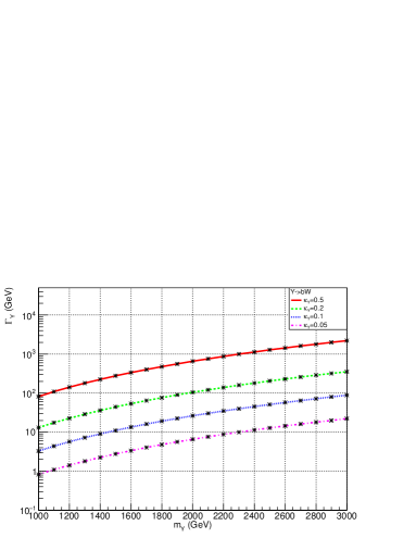
Figure 1: Decay width for vectorlike $Y$ quark depending on the mass $m_{Y}$ for different value of the coupling parameter $\kappa_{Y}$.

IV Production Cross Section

In order to make a prediction for the signal, we calculate cross section for on-shell vectorlike $Y$ quark production. Here, we consider $pp\to Ybj+X$ signal process for investigating interactions between vectorlike $Y$ quark and SM bottom quark via $W$ boson specified in Eq. 1. The representative diagram for the subprocess $qg\to Y\bar{b}q^{\prime}$ (a similar diagram for $\bar{Y}$ single production) with subsequent decays $Y\to W^{-}b\to q\bar{q}^{\prime}b$ is presented in Fig. 2. It is representative for the brevity, because there are a lot of signal diagrams for both $Y\bar{b}j$ and $\bar{Y}bj$ productions, corresponding to the $W^{\pm}$ exchange, light quark flavors $q$ and $q^{\prime}$, $b$-quark and anti $b$-quark, which we take them into account in the event generation.

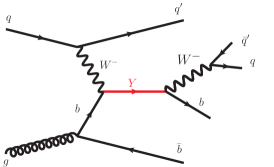
Figure 2: Representative diagram for single production of vectorlike $Y$ quark with subsequent hadronic decay channel.

The cross section for single production of vectorlike $Y$ quark through the process $pp\to Ybj+X$ depending on different mass $m_{Y}$ and coupling values $\kappa_{Y}$ has been presented in Fig. 3. As it can be seen from this figure, the cross section has large values especially in the low mass region and it increases depending on the increase in coupling parameters. In more detail, we present the signal cross section for different mass $m_{Y}=1000,1500,2000,2500$ GeV and coupling parameter values $\kappa_{Y}=0.5,0.2,0.1,0.05$ in Table A.1. We present cross section numerical values in the Appendix A to avoid similar information as in Fig. 3. The cross section decreases according to the decreasing values of coupling parameter $\kappa_{Y}$ and to the increasing values of the mass $m_{Y}$. While making these cross section calculations, we take into account automatic calculation (auto) mode of decay width $\Gamma_{Y}$. In the single production of vectorlike $Y$ quark, which is model dependent, the cross section can be related to a function of coupling $\kappa_{Y}$ and mass $m_{Y}$ within the model framework.

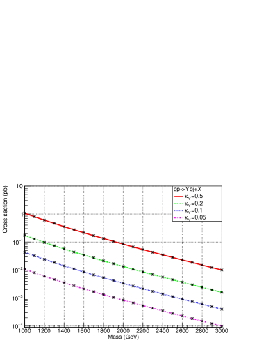
Figure 3: Cross section for the process $pp\to Ybj+X$ depending on the mass of vectorlike $Y$ quark for different coupling values.

V Modeling of Signal and Background

The signal samples are generated with the MadGraph5_aMC@NLO (key-10, ) using VLQ_V4_4FNS_UFO model implemented in FeynRules (key-11, ; key-12, ), through single production $pp\to Ybj$ as a high mass on-shell particle $Y$ with left-handed or right-handed couplings and subsequent decays $Y\to Wb$ followed by $W$ boson decaying hadronically. However, the kinematics of the final-state jets are similar for left-handed ($\kappa_{bL}^{Y}$) and right-handed ($\kappa_{bR}^{Y}$) couplings, then the acceptances for two chiralities are found to be the same. All hadronic channel is optimised to search for massive vectorlike $Y$ quark which decays to a $W$ boson and a high-momentum $b$-jet in the final state. The $W$-boson and the $b$-jet originating from the vectorlike $Y$ quark decay are expected to be back-to-back in the transverse plane. The signal topology includes an outgoing light quark in the process which often produces a forward jet in the detector. The second $b$-jet in the signal events comes from the gluon to a pair of $b$-quark ($b\bar{b}$) splitting which may be observed in either the forward or central region. Having typically low momentum, it is often assumed to be outside of the detector acceptance.

Signal and background cross sections are given in Table 1. The SM background simulation samples include top quark pair $t\bar{t}$, $W+jets$, $Z+jets$, single top quark ($tj,$ $tb$, $tW$), associate top and $Z$ production ($tZj$), $WW$, $ZZ$ and $WZ$ dibosons. The events for these processes are generated with MadGraph5_aMC@NLO (key-10, ). Monte Carlo event simulations for SM background and signal are interfaced with Pythia8 (key-13, ) for fragmentation and showering. Signal and background samples use the NNPDF2.3 PDF set (key-14, ). Both the signal and background events are produced with the generator level cuts: such as minimum transverse momentum of jets $p_{T}(j)=20$ GeV, maximum pseudo-rapidity for jets $|\eta(j)|=5$, and minimum distance between jets $\Delta R(j,j)=0.4$.

Table 1: Process, mode and generated jets in modeling the signals and different backgrounds, and calculated cross sections. While calculating these cross sections, the $W/Z$ boson and top quark are allowed to decay hadronically.

Process	Mode	Gen jets	Cross Section (pb)
$\kappa_{Y}=0.5$, $m_{Y}=1000\text{ GeV}$	$Ybj$	$2b+3j$	$6.499\times 10^{-1}$
$\kappa_{Y}=0.5$, $m_{Y}=1500\text{ GeV}$	$Ybj$	$2b+3j$	$1.520\times 10^{-1}$
$\kappa_{Y}=0.5$, $m_{Y}=2000\text{ GeV}$	$Ybj$	$2b+3j$	$4.160\times 10^{-2}$
$\kappa_{Y}=0.5$, $m_{Y}=2500\text{ GeV}$	$Ybj$	$2b+3j$	$1.236\times 10^{-2}$
$\kappa_{Y}=0.3$, $m_{Y}=500\text{ GeV}$	$Ybj$	$2b+3j$	$1.422\times 10^{0}$
$\kappa_{Y}=0.3$, $m_{Y}=1000\text{ GeV}$	$Ybj$	$2b+3j$	$2.367\times 10^{-1}$
$\kappa_{Y}=0.3$, $m_{Y}=1500\text{ GeV}$	$Ybj$	$2b+3j$	$5.909\times 10^{-2}$
$\kappa_{Y}=0.3$, $m_{Y}=2000\text{ GeV}$	$Ybj$	$2b+3j$	$1.734\times 10^{-2}$
$\kappa_{Y}=0.15$, $m_{Y}=500\text{ GeV}$	$Ybj$	$2b+3j$	$3.531\times 10^{-1}$
$\kappa_{Y}=0.15$, $m_{Y}=1000\text{ GeV}$	$Ybj$	$2b+3j$	$5.931\times 10^{-2}$
$\kappa_{Y}=0.15$, $m_{Y}=1500\text{ GeV}$	$Ybj$	$2b+3j$	$1.513\times 10^{-2}$
$\kappa_{Y}=0.15$, $m_{Y}=2000\text{ GeV}$	$Ybj$	$2b+3j$	$4.583\times 10^{-3}$
$t\bar{t}$	$t\bar{t}$	$2b+4j$	$2.174\times 10^{2}$
$SingleTop$	$tj$	$b+3j$	$1.346\times 10^{2}$
	$tb$	$2b+2j$	$4.436\times 10^{0}$
	$tW$	$b+4j$	$9.267\times 10^{-2}$
$tZj$	$tZj$	$b+5j$	$1.040\times 10^{-2}$
$Dibosons$	$WW$	$4j$	$2.775\times 10^{1}$
	$WZ$	$4j$	$8.341\times 10^{0}$
	$ZZ$	$4j$	$2.529\times 10^{0}$
$W+jets$	$W+j$	$3j$	$2.540\times 10^{4}$
	$W+2j$	$4j$	$1.062\times 10^{4}$
	$W+3j$	$5j$	$4.329\times 10^{3}$
	$W+bj$	$b+3j$	$4.564\times 10^{0}$
	$W+bjj$	$b+4j$	$1.881\times 10^{0}$
$Z+jets$	$Z+j$	$3j$	$6.476\times 10^{3}$
	$Z+2j$	$4j$	$2.668\times 10^{3}$
	$Z+3j$	$5j$	$1.086\times 10^{3}$
	$Z+bj$	$b+3j$	$9.010\times 10^{-3}$
	$Z+bjj$	$b+4j$	$9.828\times 10^{-3}$

The signal process $pp\rightarrow Ybj$ (which includes both $Y$ and $\bar{Y}$ VLQs, as well as $b$ and $\bar{b}$ quarks) process suffers from various backgrounds and one of them is clearly $t\bar{t}$ production process. When considering production and all hadronic decays, the $t\bar{t}$ process mimics the most characteristic feature of the signal process which leads the existence of two b-jets $(t\bar{t}\rightarrow W^{+}bW^{-}\bar{b}\to 4j+2b)$.

$t\bar{t}$ pair production is an important background in most BSM searches. Top quark pairs generally decay into two $W$ bosons and a pair of $b$ quarks. Then, the final state contains at least six hadronic jets. Moreover due to the high cross section of the $t\bar{t}$ background, it shows presence at every relevant region and resembles in many aspects of signal process, hence it must be trimmed by applying proper event selection and analysis cuts. $t\bar{t}$ background and signal processes differ in some respects such as the existence of more energetic jets and higher hadronic transverse energy for the signal. However, presence of two top quarks with high cross section is obviously problematic. As a direct consequence of this result, we expect an affection at top mass reconstruction. Hence our cuts are decided to reduce its dominance.

Single top production also matters and needed to be handled well using proper cuts. Since it has large cross section and some modes of that background are very close to signal process besides due to high mass of top quark, mass reconstruction for these processes resemble in some aspects with the signal. Single top quark production $tq$, $tb$ and $tW$ samples, in which top quark decays to a $W$ boson (decaying hadronically) and a $b$ quark ($t\rightarrow Wb\rightarrow q\bar{q^{\prime}}b$), have been produced. The $tZj$ sample has been produced with the top quark decaying hadronically ($t\rightarrow Wb\rightarrow q\bar{q^{\prime}}b$) and $Z$ boson decaying to two quarks ($Z$$\rightarrow q\bar{q}$($q\neq b$)).

We produce $W$+$jets$ and $Z$+$jets$ samples which include only hadronic $W$ or $Z$ boson decays, and a hadronic transverse energy cut $H_{T}>400$ GeV (where $H_{T}$ is the scalar sum of transverse momentum of selected jets) is applied in the analysis to reduce these background.

The dibosons $WW$, $ZZ$ and $WZ$ samples have been generated with hadronic decays leading at least four hadronic jets, which can be suppressed according to the selections of two jets invariant mass interval.

At largely, the backgrounds mentioned after single top are less problematic. Although some of them have large cross sections, with the invariant mass reconstruction, cut down on the signal dominant region. Futhermore, transverse momentum of the leading jet have significantly different behaviour for the signal. On the whole, background can be kept under control especially at high mass region.

The detector response to the signal and background events is simulated using a detailed description of the HL-LHC detector card implementation in Delphes v3.4 (key-15, ). All events are analyzed by developing an analysis macro with Root v6 (key-16, ) . The kinematical distributions are normalized to the number of events, which is defined to be the cross-section times luminosity for each process under consideration.

VI Analysis And Results

The analysis targets $Wb$ events with $W$ boson decaying hadronically in order to reconstruct vectorlike $Y$ quarks (full hadronic mode: $Y\to bW\to bjj$). In this mode event selection requires at least five jets and at least one of them being $b$-tagged, where hadronically decaying $W$ boson identified from dijet invariant mass. Our all hadronic analysis focuses on final states at least five (small radius) jets, one of them can be identified as forward jet and one of the $b$-tagged jet can be considered collinear jet, other two jets can be considered as central jets reconstructing the $W$ boson mass. These two jets together with one leading ($b$-tagged) jet reconstruct vectorlike $Y$ quark invariant mass. The final discriminant variables are chosen as leading jet $p_{T}$, hadronic transverse energy $H_{T}$ (We define $H_{T}$ as the hadronic activity typically associated with single vectorlike $Y$ quark production, where this variable is defined as the scalar sum of the transverse momentum of selected jets in the events.), and the reconstructed mass $m_{Y}$ of the vector like $Y$quark candidate.

The normalized distributions of the number of jets in signal events (with mass $m_{Y}=1500$ GeV and coupling $\kappa_{Y}=0.5$), and also in the relevant backgrounds are given in Fig. 4. The signal has mostly four and five jets in the final state, while the background $tZj$ and $t\bar{t}$ dominates in this region, event selection with the requirement $n_{jet}\geqslant 5$ reduce other backgrounds.

Figure 4: The normalized distribution of the number of jets (jet size) for signal (with $m_{Y}=1500$ GeV and $\kappa_{Y}=0.5$), and also for the relevant backgrounds in all hadronic channels.

One of the important background for our analysis is the top pair production $t\bar{t}$ due to its high cross section. Here, we give the $p_{T}$ and $\eta$ distributions of the jets ($p_{T}$ ordered) for this process without any cuts to reflect it’s main characteristics. Hence, we have the chance to exploit its main differences. As we can see from a quick comparison between the signal distributions, discriminating differences occur at the distributions of the high $p_{T}$ jets.

The transverse momentum ($p_{T}$) and pseudo-rapidity ($\eta$) distributions of five jets for signal, for $m_{Y}=1500$ GeV and $m_{Y}=2000$ GeV ($\kappa_{Y}=0.5$ for both) and also for top pair, associated $tZj$ production, single top, $W$+$jets$, $Z$+$jets$ and dibosons background are presented in Fig. A.1 - A.8, respectively.

The transverse momentum ($p_{T}$) and pseudo-rapidity ($\eta$) distributions of jets for $W+jets$ (including $W+j,W+2j,W+3j,W+bj,W+bjj$) background are presented in Fig. A.6. The generator level cuts are applied to these kinematic distributions of the final state jets. Comparing the signal and the $W+jets$ background distributions, it can be seen that 1st and 2nd jets have different distributions of the $p_{T}$ and $\eta$. A similar discussion is also valid for the $Z+jets$ background when the hadronic mode is considered.

The transverse momentum and pseudo-rapidity distributions of all jets for whole diboson background (including $WW,WZ,ZZ$) before performing the cuts are shown in Fig. A.8. As it can be seen from Fig. A.8, the pseudo-rapidity distribution of the jets are symmetrical with respect to the beam axis and the tails of the distribution for the 5th jet are getting longer in both forward and backward direction. The transverse momentum distribution falls rapidly for high $p_{T}$ values.

In addition to the $p_{T}$ and $\eta$ cuts on the selected final state jets, a transverse hadronic energy cut $H_{T}>400$ GeV is applied in the analysis, where $H_{T}$ is the scalar sum of the $p_{T}$ of all selected jets. The angular distance (or angular separation) between two jets defines how much two jets are moving in the same direction, and it is usually denoted as $\Delta R=\sqrt{\Delta\eta^{2}+\Delta\phi^{2}}$, where a cut $\Delta R(j,j)>0.4$ is applied to the selected events. The preselection and cut flow for the analysis are given in Table 2.

Cut efficiencies ($\%$) for different signal benchmarks ($\kappa_{Y}=0.5$ and $m_{Y}=1000$, $1500$, $2000,$ $2500$ GeV) and backgrounds in Table 3 have been obtained by applying the cuts explained in Table 2, where the leading jet $p_{T}$ variable has been used.

The invariant mass distribution $m_{Y}$ for all signals and background are presented in Fig. 5. The leading jet $p_{T}$ distributions for all signals and backgrounds are shown in Fig. 6. The scalar sum $p_{T}$ for all signals and backgrounds are shown in Fig. A.9. The ratio of the scalar sum $p_{T}$ to the total scalar $H_{T}$, $H_{T}^{R}$, in the event is shown in Fig. 7. Fig. 8 and Fig. 9 show the invariant mass distributions of the vectorlike $Y$quark for $\kappa_{Y}=0.3$ and $\kappa_{Y}=0.15$, respectively. The distributions shown in Fig. 5-9 and Fig. A.9 are normalized to the expected number of events, defined as the cross-section of related process multiplied by the integrated luminosity of $L_{int}=1000$ fb^-1.

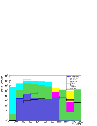
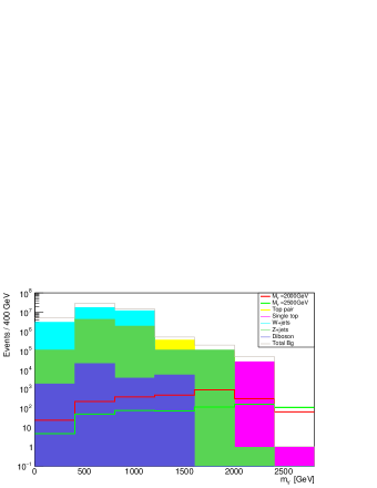
Figure 5: The invariant mass distribution $m_{Y}$ for all signals ($\kappa_{Y}=0.5$) and backgrounds. For $m_{Y}=1000$ and $1500$ GeV (upper), for $m_{Y}=2000$ and $2500$ GeV (lower).

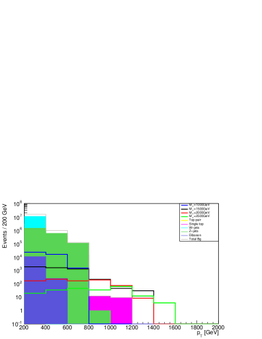
Figure 6: The leading jet $p_{T}$ distributions for all signals ($\kappa_{Y}=0.5$) and backgrounds.

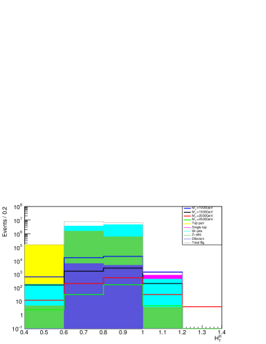
Figure 7: The ratio of the scalar sum $p_{T}$ to the total scalar $H_{T}$. $\kappa_{Y}=0.5$ for all signals.

Figure 8: The invariant mass distribution $m_{Y}$ for all signals ($\kappa_{Y}=0.3$) and backgrounds. For $m_{Y}=500$ and $1000$ GeV (upper), for $m_{Y}=1500$ and $2000$ GeV (lower).

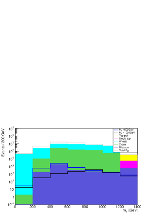
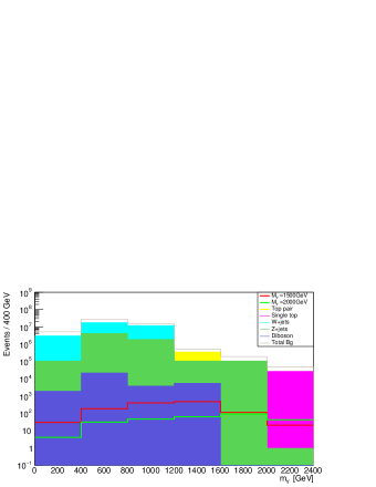
Figure 9: The invariant mass distribution $m_{Y}$ for all signals ($\kappa_{Y}=0.15$) and backgrounds. For $m_{Y}=500$ and $1000$ GeV (upper), for $m_{Y}=1500$ and $2000$ GeV (lower).

Table 2: Preselection and set of cuts for the analysis of signal and background events.

Cuts	Definition
Cut-0	Preselection: number of jets $N_{j}\geqslant 5$
Cut-1	Leading jet $p_{T}>200$ GeV and $|\eta|<2.0$
	Collinear jet $p_{T}>30$ GeV and $|\eta|<3.0$
	Other jets $p_{T}>30$ GeV and $|\eta|<2.5$
Cut-2	Number of b tagged jet $N_{b}\geqslant 1$
Cut-3	Angular separation between two jets $\Delta R(j,j)>0.4$
Cut-4	Scalar sum of $p_{T}$ of jets $H_{T}>400$ GeV
Cut-5	Invariant mass interval of two jets $|m_{jj}-m_{W}|<20$ GeV
Cut-6	Invariant mass interval of three jets $|m_{bjj}-m_{Y}|<0.2m_{Y}$ GeV

Table 3: Cut efficiencies (%) for different signal benchmarks ( $\kappa_{Y}=0.5$ and $m_{Y}=1000,1500,2000,2500$ GeV) and backgrounds.

	Cut-1	Cut-2	Cut-3	Cut-4	Cut-5
$m_{Y}=1000$ GeV	$30.28$	$25.20$	$25.03$	$25.03$	$7.60$
$m_{Y}=1500$ GeV	$30.41$	$24.42$	$24.35$	$24.35$	$4.09$
$m_{Y}=2000$ GeV	$31.84$	$25.31$	$25.27$	$25.27$	$2.58$
$m_{Y}=2500$ GeV	$33.52$	$25.71$	$25.71$	$25.71$	$2.15$
$t\bar{t}$	$6.58$	$4.14$	$4.14$	$4.14$	$2.09$
$tb$	$7.63$	$6.80$	$6.71$	$6.71$	$3.22$
$tW$	$13.78$	$6.31$	$6.28$	$6.28$	$3.02$
$tj$	$2.88$	$1.87$	$1.87$	$1.87$	$1.01$
$tZj$	$8.37$	$4.25$	$4.25$	$4.25$	$1.72$
$Wbj$	$3.13$	$2.30$	$2.30$	$2.30$	$0.21$
$Wbjj$	$4.48$	$2.65$	$2.65$	$2.65$	$0.71$
$Wj$	$1.83$	$0.61$	$0.61$	$0.61$	$0.61$
$Wjj$	$4.53$	$0.40$	$0.40$	$0.40$	$0.10$
$Wjjj$	$6.65$	$0.76$	$0.76$	$0.76$	$0.27$
$Zbj$	$6.67$	$3.74$	$3.74$	$3.74$	$1.72$
$Zbjj$	$11.22$	$5.83$	$5.83$	$5.83$	$2.49$
$Zj$	$3.29$	$0.00$	$0.00$	$0.00$	$0.00$
$Zjj$	$4.51$	$0.88$	$0.88$	$0.88$	$0.10$
$Zjjj$	$6.53$	$0.69$	$0.69$	$0.69$	$0.20$
$WW$	$7.10$	$0.81$	$0.81$	$0.81$	$0.00$
$ZZ$	$5.03$	$0.41$	$0.41$	$0.41$	$0.27$
$WZ$	$5.54$	$0.66$	$0.66$	$0.66$	$0.66$

For calculating signal significance ($SS$) as incorporated in (key-17, ; key-18, ; key-19, ), we use the invariant mass interval defined as $|m_{bjj}-m_{Y}|<0.2m_{Y}$. The expected signal significance is given in terms of signal ($S$) and background events ($B$).

In the special case of well known background, the statistical significance ($SS$)

$$SS=\sqrt{2\left[(S+B)\ln\left(1+\frac{S}{B}\right)-S\right]}$$

which would further reduces to $S/\sqrt{B}$ in the limit of large background events. The signal significances for the couplings $\kappa_{Y}=0.5$, $\kappa_{Y}=0.3$ and $\kappa_{Y}=0.15$ at the projected integrated luminosities of $L_{int}=300$ fb^-1, $1000$ fb^-1 and $3000$ fb^-1 are given in Table 3, 4 and 5, respectively. These results are obtained for the invariant mass $m_{Y}$ variable after applying the cuts as in Table 2 to all signals and backgrounds event samples.

Table 4: Statistical significance ($SS$) for different signal benchmarks ( $\kappa_{Y}=0.5$ and $m_{Y}=1000,1500,2000,2500$ GeV) and different integrated luminosity projections at HL-LHC.

Signal	$L_{int}($fb-1)
	$300$	$1000$	$3000$
$\kappa_{Y}=0.5$, $m_{Y}=1000\text{ GeV}$	$9.13$	$16.67$	$28.88$
$\kappa_{Y}=0.5$, $m_{Y}=1500\text{ GeV}$	$3.73$	$6.80$	$11.78$
$\kappa_{Y}=0.5$, $m_{Y}=2000\text{ GeV}$	$1.33$	$2.43$	$4.21$
$\kappa_{Y}=0.5$, $m_{Y}=2500\text{ GeV}$	$0.50$	$0.92$	$1.59$

Table 5: The same as Table 4, but for $\kappa_{Y}=0.3$ and $m_{Y}=500,1000,1500,2000$ GeV.

Signal	$L_{int}($fb-1)
	$300$	$1000$	$3000$
$\kappa_{Y}=0.3$, $m_{Y}=500\text{ GeV}$	$13.54$	$24.73$	$42.83$
$\kappa_{Y}=0.3$, $m_{Y}=1000\text{ GeV}$	$3.22$	$5.88$	$10.18$
$\kappa_{Y}=0.3$, $m_{Y}=1500\text{ GeV}$	$0.72$	$1.32$	$2.28$
$\kappa_{Y}=0.3$, $m_{Y}=2000\text{ GeV}$	$0.50$	$0.92$	$1.59$

Table 6: The same as Table 4, but for $\kappa_{Y}=0.15$ and $m_{Y}=500,1000,1500,2000$ GeV.

Signal	$L_{int}($fb-1)
	$300$	$1000$	$3000$
$\kappa_{Y}=0.15$, $m_{Y}=500\text{ GeV}$	$3.60$	$6.58$	$11.39$
$\kappa_{Y}=0.15$, $m_{Y}=1000\text{ GeV}$	$0.77$	$1.41$	$2.45$
$\kappa_{Y}=0.15$, $m_{Y}=1500\text{ GeV}$	$0.17$	$0.31$	$0.53$
$\kappa_{Y}=0.15$, $m_{Y}=2000\text{ GeV}$	$0.15$	$0.28$	$0.48$

The statistical significance $SS$ as a function of mass of vectorlike $Y$ quark for $L_{int}=300$ fb^-1, $1000$ fb^-1 and $3000$ fb^-1 are shown in Fig. 10, 11 and 12. In these figures, the coupling values $\kappa_{Y}=0.5$, $\kappa_{Y}=0.3$ and $\kappa_{Y}=0.15$ are chosen as benchmarks, respectively. For the integrated luminosity projection of $3000$ fb^-1, lower limits for $m_{Y}$ are obtained as $2350$ GeV at $2\sigma$ significance level, $2150$ GeV at $3\sigma$ (observability) and $1900$ GeV at $5\sigma$ (discovery) significances. For other couplings $\kappa_{Y}=0.3$ and $\kappa_{Y}=0.15$ the lower limits for $m_{Y}$ are found as $1550$ GeV and $1075$ GeV at $2\sigma$ significance level at $L_{int}=3000$ fb^-1, respectively.

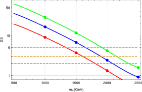
Figure 10: The statistical significance $SS$ for $\kappa_{Y}=0.5$ as a function of vectorlike $Y$ quark mass $m_{Y}$ for integrated luminosity projections (solid lines, red to green) $L_{int}=300$ fb^-1, $1000$ fb^-1 and $3000$ fb^-1 at HL-LHC. The horizontal dashed lines correspond to $2\sigma$, $3\sigma$ and $5\sigma$ significances (lower to upper), respectively.

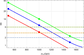
Figure 11: The same as Fig. 10, but for $\kappa_{Y}=0.3$.

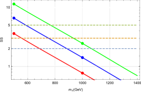
Figure 12: The same as Fig. 10, but for $\kappa_{Y}=0.15$.

VII Conclusions

We have studied single production of vectorlike $Y$ quark and its subsequent decay ($Y\to Wb$) with phenomenological interpretations in the context of well motivated VLQ model framework. Signal significances have been obtained depending on the parameter space (mass in the range $1000-2500$ GeV for coupling $\kappa_{Y}=0.5$ and $500-2000$ GeV for couplings $\kappa_{Y}=0.3$ and $\kappa_{Y}=0.15$) using all hadronic mode (at least five jets final state). We find a significant coverage of the signal parameter space and distinguish the signal for a mass up to $2350$ GeV for an integrated luminosity of $3000$ fb^-1 at the HL-LHC. We have used the criteria for projected discovery (key-20, ) sensitivities to the couplings and masses. For signal significance $2\sigma$ level we find vectorlike $Y$ quark attainable mass limits as $1800$ GeV, $2100$ GeV and $2350$ GeV at projected integrated luminosities $L_{int}=300$ fb${}^{-1},$$1000$ fb^-1 and $3000$ fb^-1, respectively. For other coupling values $\kappa_{Y}=0.3$ ($\kappa_{Y}=0.15$) we find attainable mass limits as $1150$ GeV ($700$ GeV), $1350$ GeV ($900$ GeV) and $1550$ GeV ($1075$ GeV) at the same integrated luminosity projections. The systematics are known to affect the discovery reaches. However, given the difficulty to perform a precise estimation of systematics for projected results, the significances have been computed without considering the systematic uncertainties (an optimistic case) for the estimation of the potential of HL-LHC. These results can also be used for constraining the models (key-21, ; key-22, ) predicting new heavy quarks with exotic charge as $-4/3$. This analysis shows that HL-LHC could discover a wide range of parameter space of vectorlike $Y$ quark models.

Appendix A

We present following Table A.1 and Figures A.1 - A.9 to avoid detailed information in the main text.

Table A.1: The leading order (LO) signal cross section values (in pb) for the process $pp\rightarrow Ybj+X$ at the HL-LHC with $\sqrt{s}=14$ TeV.

$m_{Y}(\text{GeV})$	$\kappa_{Y}=0.5$	$\kappa_{Y}=0.2$	$\kappa_{Y}=0.1$	$\kappa_{Y}=0.05$
$1000$	$1.08\times 10^{0}$	$1.72\times 10^{-1}$	$4.30\times 10^{-2}$	$1.08\times 10^{-2}$
$1100$	$8.01\times 10^{-1}$	$1.28\times 10^{-1}$	$3.21\times 10^{-2}$	$8.01\times 10^{-3}$
$1200$	$6.04\times 10^{-1}$	$9.63\times 10^{-2}$	$2.42\times 10^{-2}$	$6.04\times 10^{-3}$
$1300$	$4.61\times 10^{-1}$	$7.37\times 10^{-2}$	$1.85\times 10^{-2}$	$4.60\times 10^{-3}$
$1400$	$3.55\times 10^{-1}$	$5.68\times 10^{-2}$	$1.41\times 10^{-2}$	$3.55\times 10^{-3}$
$1500$	$2.76\times 10^{-1}$	$4.41\times 10^{-2}$	$1.10\times 10^{-2}$	$2.75\times 10^{-3}$
$1600$	$2.15\times 10^{-1}$	$3.44\times 10^{-2}$	$8.56\times 10^{-3}$	$2.14\times 10^{-3}$
$1700$	$1.69\times 10^{-1}$	$2.70\times 10^{-2}$	$6.73\times 10^{-3}$	$1.69\times 10^{-3}$
$1800$	$1.33\times 10^{-1}$	$2.13\times 10^{-2}$	$5.30\times 10^{-3}$	$1.33\times 10^{-3}$
$1900$	$1.06\times 10^{-1}$	$1.69\times 10^{-2}$	$4.21\times 10^{-3}$	$1.05\times 10^{-3}$
$2000$	$8.44\times 10^{-2}$	$1.34\times 10^{-2}$	$3.37\times 10^{-3}$	$8.41\times 10^{-4}$
$2100$	$6.72\times 10^{-2}$	$1.07\times 10^{-2}$	$2.70\times 10^{-3}$	$6.71\times 10^{-4}$
$2200$	$5.39\times 10^{-2}$	$8.62\times 10^{-3}$	$2.16\times 10^{-3}$	$5.40\times 10^{-4}$
$2300$	$4.34\times 10^{-2}$	$6.95\times 10^{-3}$	$1.74\times 10^{-3}$	$4.34\times 10^{-4}$
$2400$	$3.49\times 10^{-2}$	$5.62\times 10^{-3}$	$1.40\times 10^{-3}$	$3.50\times 10^{-4}$
$2500$	$2.83\times 10^{-2}$	$4.54\times 10^{-3}$	$1.13\times 10^{-3}$	$2.84\times 10^{-4}$
$2600$	$2.29\times 10^{-2}$	$3.67\times 10^{-3}$	$9.11\times 10^{-4}$	$2.29\times 10^{-4}$
$2700$	$1.86\times 10^{-2}$	$2.98\times 10^{-3}$	$7.42\times 10^{-4}$	$1.85\times 10^{-4}$
$2800$	$1.51\times 10^{-2}$	$2.42\times 10^{-3}$	$6.02\times 10^{-4}$	$1.51\times 10^{-4}$
$2900$	$1.23\times 10^{-2}$	$1.97\times 10^{-3}$	$4.91\times 10^{-4}$	$1.23\times 10^{-4}$
$3000$	$1.01\times 10^{-2}$	$1.60\times 10^{-3}$	$4.00\times 10^{-4}$	$9.98\times 10^{-5}$

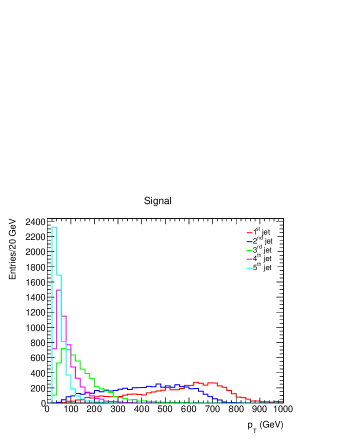
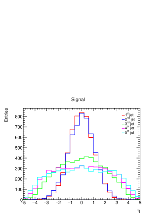
Figure A.1: Transverse momentum (upper) and pseudo-rapidity (lower) distribution of five jets for signal with $m_{Y}=1500$ GeV and $\kappa_{Y}=0.5$.

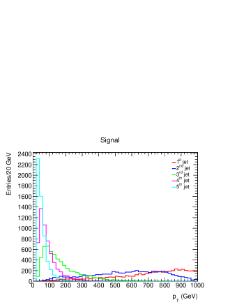
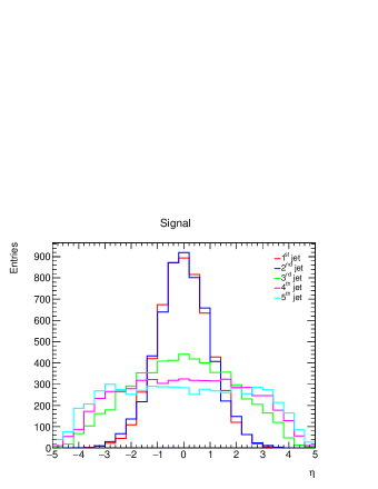
Figure A.2: The same as Fig. A.1, but for signal with $m_{Y}=2000$ GeV and $\kappa_{Y}=0.5$.

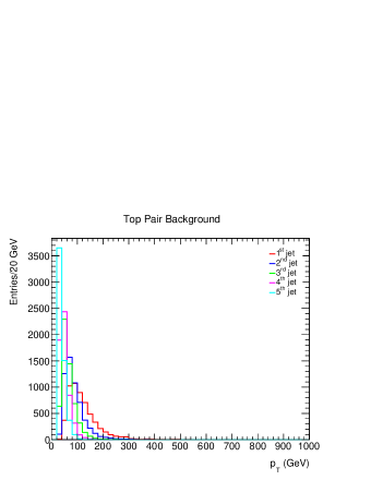
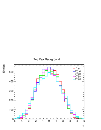
Figure A.3: Transverse momentum (upper) and pseudo-rapidity (lower) distributions of five jets for top-pair background.

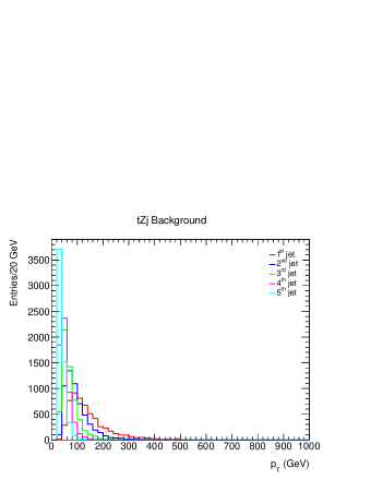
Figure A.4: Transverse momentum (upper) and pseudo-rapidity (lower) distributions of five jets for associated tZj production background.

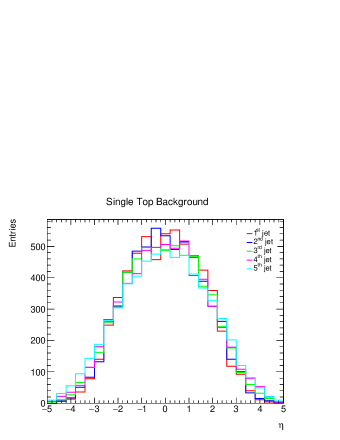
Figure A.5: Transverse momentum (upper) and pseudo-rapidity (lower) distributions of five jets for single top background.

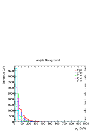
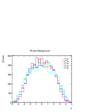
Figure A.6: Transverse momentum (upper) and pseudo-rapidity (lower) distributions of five jets for $W+jets$ background.

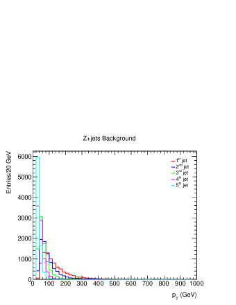
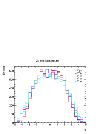
Figure A.7: Transverse momentum (upper) and pseudo-rapidity (lower) distributions of five jets for $Z+jets$ background.

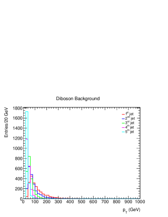
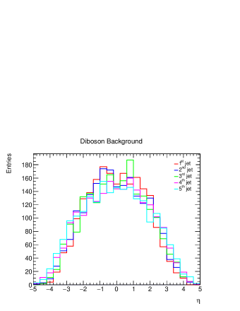
Figure A.8: Transverse momentum (upper) and pseudo-rapidity (lower) distributions of five jets for diboson background.

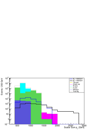
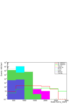
Figure A.9: The scalar sum $p_{T}$ for all signals ($\kappa_{Y}=0.5$) and backgrounds. For $m_{Y}=1000$ and $1500$ GeV (upper), for $m_{Y}=2000$ and $2500$ GeV (lower).

References

- (1) Apollinari G et al. 2017 High-Luminosity Large Hadron Collider (HL-LHC) Technical Design Report V. 0.1 (Geneva: CERN). https://doi.org/10.23731/CYRM-2017-004.
- (2) M. Buchkremer, G. Cacciapaglia, A. Deandrea, L. Panizzi, Model Independent Framework for Searches of Top Partners, hep-ph/1305.4172.
- (3) J. A. Aguilar-Saavedra, R. Benbrik, S. Heinemeyer and M. Perez-Victoria, Handbook of vectorlike quarks: Mixing and single production, Phys. Rev. D 88 (2013) 094010, arXiv: 1306.0572 [hep-ph].
- (4) ATLAS Collaboration, Search for single production of vectorlike quarks decaying into Wb in pp collisions at TeV with the ATLAS detector, JHEP05, 164 (2019).
- (5) CMS Collaboration, Search for single production of vectorlike quarks decaying into a b quark and a W boson in proton–proton collisions at TeV, Physics Letters B 772, 634-656 (2017).
- (6) Alexandra Carvalho, Stefano Moretti, Dermot O’Brien, Luca Panizzi, Hugo Prager, Single production of vector like quarks with large width at the Large Hadron Collider, Phys.Rev. D 98, 015029 (2018).
- (7) Aldo Deandrea, Thomas Flacke, Benjamin Fuks, Luca Panizzi and Hua-Sheng Shaoc, Single production of vector-like quarks: the effects of large width, interference and NLO corrections, JHEP08(2021)107.
- (8) J. A. Aguilar-Saavedra, Mixing with vectorlike quarks: constraints and expectations, EPJ Web Conf. 60 (2013) 16012, arXiv: 1306.4432 [hep-ph].
- (9) Benjamin Fuks, Hua-Sheng Shao, QCD next-to-leading-order predictions matched to parton showers for vectorlike quark models, Eur. Phys. J. C (2017) 77:135. arXiv: 1610.04622 [hep-ph]
- (10) J. Alwall, R. Frederix, S. Frixione, V. Hirschi, F. Maltoni, O. Mattelaer, H.-S. Shao, T. Stelzer, P. Torrielli, M. Zaro, The automated computation of tree-level and next-to-leading order differential cross sections, and their matching to parton shower simulations, arXiv:1405.0301 [hep-ph].
- (11) A. Alloul, N.D. Christensen, C. Degrande, C. Duhr, B. Fuks, FeynRules 2.0 — A complete toolbox for tree-level phenomenology, Computer Physics Communications Volume 185, Issue 8, Pages: 2250-2300, (2014).
- (12) C. Degrande, C. Duhr, B. Fuks, D. Grellscheid, O. Mattelaer, T. Reiter, UFO – The Universal FeynRules Output, Computer Physics Communications, Volume 183, Issue 6, Pages: 1201-1214, (2012).
- (13) Torbjörn Sjöstrand, Stefan Ask, Jesper R. Christiansen, Richard Corke, Nishita Desai, Philip Ilten, Stephen Mrenna, Stefan Prestel, Christine O. Rasmussen, Peter Z. Skand, An introduction to PYTHIA 8.2, Computer Physics Communications, Volume 191, Pages 159-177 (2015).
- (14) R.D. Ball et al., Parton distributions with LHC data, Nucl. Phys. B 867 (2013) 244 [arXiv:1207.1303] [Inspire].
- (15) J. de Favereau, C. Delaere, P. Demin, A. Giammanco, V. Lematre, A. Mertens and M. Selvaggi, “Delphes 3, A modular framework for fast simulation of a generic collider experiment”, arXiv:1307.6346 [hep-ex].
- (16) R. Brun, F. Rademakers, Nuclear instruments and methods in physics research section A: accelerators, spectrometers, detectors and associated equipment. New Comput. Techn. Phys. Res. V 389, 81 (1997). https://doi.org/10.1016/S0168-9002(97)00048-X.
- (17) G. Cowan, K. Cranmer, E. Gross and O. Vitells, Asymptotic formulae for likelihood-based tests of new physics”, Eur. Phys. J. C 71, 1554 (2011) [Eur. Phys. J. C 73, 2501 (2013)] [arXiv:1007.1727 [physics.data-an]].
- (18) Robert D. Cousins, James T. Linnemann, Jordan Tucker, Evaluation of three methods for calculating statistical significance when incorporating a systematic uncertainty into a test of the background-only hypothesis for a Poisson process, Nuclear Instruments and Methods in Physics Research A 595 (2008) 480–501.
- (19) G. Cowan, “Two developments in tests for discovery: use of weighted Monte Carlo events and an improved measure”, Progress on Statistical Issues in Searches”, SLAC”, June 4 - 6, 2012.
- (20) P. N. Bhattiprolu, S.P. Martin, James D. Wells, Criteria for projected discovery and exclusion sensitivities of counting experiments, arXiv:2009.07249 [physics.data-an].
- (21) D. Chang, W. Chang, and E. Ma, Alternative interpretation of the Fermilab Tevatron top events, Phys. Rev. D 59, 091503 (1999.
- (22) D. Chang, W. Chang, and E. Ma, Fitting precision electroweak data with exotic heavy quarks, Phys. Rev. D 61, 037301 (2000).