Chapter 0 SDN helps Big-Data to optimize access to data

This chapter introduces the state-of-the-art in the emerging area of combining High Performance Computing (HPC) with Big Data Analysis. To understand the new area, the chapter first surveys the existing approaches to integrating HPC with Big Data. Next, the chapter introduces several optimization solutions that focus on how to minimize the data transfer time from computation-intensive applications to analysis-intensive applications as well as minimizing the end-to-end time-to-solution. The solutions utilize SDN to adaptively use both high speed interconnect network and high performance parallel file systems to optimize the application performance. A computational framework called DataBroker is designed and developed to enable a tight integration of HPC with data analysis. Multiple types of experiments have been conducted to show different performance issues in both message passing and parallel file systems and to verify the effectiveness of the proposed research approaches.

1 Introduction

Alongside experiments and theories, computational modeling/simulation and big data analytics have established themselves as the critical third and fourth paradigms in modern scientific discovery [3, 5]. Nowadays, there is an inevitable trend towards integrating different applications of computation and data analysis together. The benefits of combining them are significant: (1) The overall end-to-end time-to-solution can be reduced considerably such that interactive or real-time scientific discovery becomes feasible; (2) the traditional one-way communication (from computation to analysis) can be bidirectional to enable guided computational modeling and simulation; and 3) computational modeling/simulation and data-intensive analysis are complementary to each other and can be used in a virtuous circle to amplify their collective effect.

However, it is a challenging task to integrate computation with analysis effectively. Critical questions include: How to minimize the cost to couple computation and analysis? how to design an effective software system to enable and facilitate such an integration? and how to optimize the co-scheduling of different computation and data-intensive applications? In this chapter, we build an analytical model to estimate the overall execution time of the integrated computation and data analysis, and design an intelligent data broker to intertwine the computation stage and the analysis stage to achieve the optimal time-to-solution predicted by the analytical model.

To fully interleave computation with analysis, we propose and introduce a fine-grain-block task-based asynchronous parallel execution model. The execution model utilizes the abstraction of pipelining, which is widely used in computer architectures [16]. In a traditional scientific discovery, a user often executes the computation, stores the computed results to disks, then reads the computed results, and finally performs data analysis. From the user’s perspective, the total time-to-solution is the sum of the four execution times. In this chapter, we rethink of the problem by using a novel method of fully asynchronous pipelining. With the asynchronous pipeline method (detailed in Section 4), a user input is divided into fine-grain blocks. Each fine-grain block goes through four steps: computation, output, input, and analysis. As shown in Figure 1, our new end-to-end time-to-solution is equal to the maximum of the the computation time, the output time, the input time, and the analysis time (i.e., the time of a single step only) [8]. Furthermore, we build an analytical model to predict the overall time-to-solution to integrate computation and analysis, which provides developers with an insight into how to efficiently combine them.

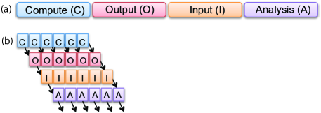
Figure 1: Comparison between the traditional process (a) and the new fully asynchronous pipeline method (b).

Although the analytical model and its performance analysis reveal that the corresponding integrated execution can result in high performance, there is no software available to support the online tight coupling of analysis and computation at run time. To facilitate the asynchronous integration of computation and analysis, we design and develop an I/O middleware, named Intelligent DataBroker, to adaptively prefetch and manage data in both secondary storage and main memory to minimize the I/O cost. This approach is able to support both in-situ (or in memory) data processing and post-processing where initial dataset is preserved for the entire community (e.g., the weather community) for subsequent analysis and verification. The computation and analysis applications are coupled up through the DataBroker. DataBroker consists of two parts: a DataBroker producer in the compute node to send data, and a DataBroker consumer in the analysis node to receive data. It has its own runtime system to provide dynamic scheduling, pipelining, hierarchical buffering, and prefetching. This chapter introduces the design of the current prototype of DataBroker briefly.

We performed experiments on BigRed II (a Cray system) with a Lustre parallel file system at Indiana University to verify the analytical model and compare the performance of the traditional process, an improved version of the traditional process with overlapped data writing and computation, and our fully asynchronous pipeline approach. Both synthetic applications and real-world computational fluid dynamics (CFD) applications have been implemented with the prototype of DataBroker. Based on the experiments, the difference between the actual time-to-solution and the predicted time-to-solution is less than 10%. Furthermore, by using DataBroker, our fully asynchronous method is able to outperform the improved traditional method by up to 78% for the real-world CFD application.

In the remainder of the chapter, Section 2 covers the state of the art. Section 3 compares the efficiency difference between the message passing method and the parallel file I/O method for transferring data between applications. Section 4 introduces the analytical model to estimate the time-to-solution. Section 5 presents the DataBroker middleware to enable an optimized integration approach. Section 6 verifies the analytical model and demonstrates the speedup using the integration approach. Finally, Section 7 raises a few open questions, and Section 8 summarizes the chapter.

2 State of the Art and Related Work

This section introduces the existing approaches to integrating computation with data analysis, and compares our work with related work.

The conventional approach: As shown earlier in Figure 1, the computational modeling and simulation applications [17, 10, 14] will compute and output computed results to files. Providing that the file format is known, any data analysis application can be launched to perform various types of data analysis. The advantage is that independent software projects can be developed at the same time in separate organizations. Also, the computed results can be stored and analyzed later by other analysis applications. The problem is that it is strictly sequential, which results in long end-to-end time-to-solution.

The in-situ approach: In opposite directions of the conventional approach, the in-situ approach analyzes data when the data are still resident in memory. While the I/O cost is eliminated, it has three issues [20, 5, 13]: 1) It takes a lot of effort to couple the computation code with the analysis code. Developers have to place analysis functions to the address space of the modeling/simulation application, which requires data-format conversion and good understanding of both computation and analysis domains; 2) Many real world applications are already tight on memory. Allocating memory to in-situ analysis (together with other resource contentions) will slow down both computation and analysis processes. Since analysis applications are typically less scalable than computation applications, the computation applications will be stalled due to the limited in-situ memory space; and 3) It does not support preserving data for long-term studies and the entire community for different data analyses.

The data-staging approach: Unlike the in-situ approach, which requires writing custom code and sharing the same resources, a general approach is to use data staging to place analysis on an analysis cluster or a separate partition of a supercomputer. The data-staging approach has a flexible design, in which computation and analysis can execute on the same compute node, on different compute nodes, or on different HPC systems. The approach can also minimize resource contention (e.g., CPU, memory, bus, disk) between computation and analysis processes. To support transferring data from computation to analysis, a few I/O libraries and middleware have been implemented. FlexIO [21] uses both shared memory and RDMA to support data analysis either on the same or different compute nodes. GLEAN [19] uses sockets to support data staging on analysis nodes on an analysis cluster. DataStager [2] and I/O Container [6] use RDMA to provide staging on a separate part of compute nodes. DataSpaces [7] provides a distributed virtual space and allows different processes to put/get data tuples to/from the space.

We create a new computing framework called DataBroker that is based on a data-driven data-staging service. It provides a unifying approach, which takes into account computation, output, input, and analysis as a whole, and performs global dynamic scheduling across computation and analysis to optimize the end-to-end time-to-solution. This approach also builds analytical models to estimate the performance of the integrated computation and analysis and optimizes the time-to-solution.

The new DataBroker is used to fasten analysis applications to computational applications. Different from the existing staging middleware, DataBroker can perform in-memory analysis or file-system based analysis—adaptively—without stalling the computation processes. Moreover, DataBroker focuses on fine-grain pipelining operations. There exist efficient parallel I/O libraries such as MPI-IO [18], ADIOS [1, 11], Nessie [12], and PLFS [4] to allow applications to adapt their I/O to specific file systems. We do not compete with these work. DataBroker is in the application level, which can use these techniques to optimize DataBroker’s performance.

3 Performance analysis of message passing and parallel file system I/O

In a typical scientific workflow, there are two available data transfer methods. One way is to transfer data via MPI library, which is a widely-used message-passing library on parallel computing systems. The other is to use file system via writing and reading files. Nowadays, file system has evolved a lot and becomes much faster than before. Current novel HPC systems mostly utilize high speed SSD to store temporary data into local disk, meanwhile use parallel file system to store long-term data.

Naturally, one may think file system is slow to transfer data compared with MPI messages. But with the rapid development of parallel file system and the emergence of systems equipped with SSD, it is necessary to reconsider this issue. Thus, we compare the performance of transferring data using MPI and file I/O. In order to achieve the goal, we design two sets of experiments. The first set is used to measure the time to transfer one block of data by one MPI message. The second set is used to get the time to transfer one block of data using file I/O.

The first set of MPI experiments is designed as follows. A producer process creates $n$ blocks filled with random values and sends them to a consumer processes using $n$ MPI messages. We measure the total time of MPI_Send function on each thread and assign it as the data transfer time $T_{MPI}$. Thus, the time to transfer a data block by MPI is $T_{MPI/Block}=\frac{T_{MPI}}{n}$.

The second set of file I/O experiments is described as follows. A producer process creates $n$ blocks filled with random values and writes them to disk. After the producer process has finished, a consumer process will start reading the files. We measure the total writing time $T_{Write}$ and reading time $T_{Read}$ on each thread and use their sum as the data transfer time. Thus, the time to transfer a data block by parallel file I/O is $T_{HDD/Block}=\frac{T_{Write}+T_{Read}}{n}$.

The two sets of experiments are performed on BigRed II and Comet. BigRed II is a Cray XE6/XK7 HPC system in Indiana University. It contains a Gemini interconnect network and a Lustre parallel file system named Data Capacitor II (DC2). Comet is a dedicated XSEDE cluster in San Diego Supercomputer Center. It contains hybrid fat-tree interconnect network and a Lustre parallel file system. Besides, each Comet compute node has 320 GB SSD local storage. Thus, we conduct the two sets of experiments first on BigRed II to get $T_{MPI/Block}$ and $T_{HDD/Block}$, and then on Comet to get $T_{MPI/Block}$, $T_{HDD/Block}$ and $T_{SSD/Block}$.

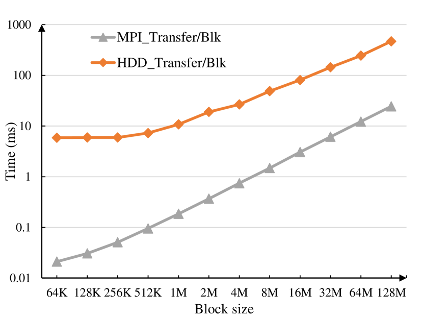
(a) Data Transfer Time via MPI and HDD

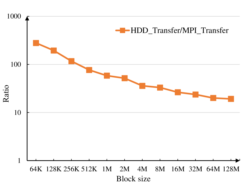
(b) Ratio of MPI/HDD

Figure 2: Data transfer Time and speedup for one block data on BigRed II.

Figure 2 (a) shows the result of $T_{MPI/Block}$ and $T_{HDD/Block}$ on BigRed II. We can observe that MPI is faster than parallel file I/O on all block sizes. In addition, both $T_{MPI/Block}$ and $T_{HDD/Block}$ will increase as the block size increases. However, the performance gap between MPI and parallel file I/O becomes gradually narrower. We use the ratio of $\frac{T_{HDD/Block}}{T_{MPI/Block}}$ to measure it. Figure 2 (b) shows that MPI outperforms parallel file I/O by 278 times on 64KB, but the ratio falls to 19 times on 128MB. This result reflects that MPI is excellent in transferring data on small block size, but the benefit loses as block size grows larger.

Figure 3 (a) shows the results on Comet. We can find that the time to transfer a data block using MPI is faster than using local SSD, and using parallel file system is the slowest. Moreover, $T_{MPI/Block}$, $T_{SSD/Block}$ and $T_{HDD/Block}$ increase as block size increases. Again, we find that the performance gap among them becomes narrower. We still use the ratio of $\frac{T_{HDD/Block}}{T_{MPI/Block}}$ and $\frac{T_{SSD/Block}}{T_{MPI/Block}}$ to measure the trend. Figure 3 (b) shows that MPI outperforms parallel file I/O by 419 times on 64KB, but the ratio drops to 17 times on 128MB. On the other hand, MPI outperforms SSD by 2.6 times on 8MB, and up to 7 times on 64KB. To transfer 128MB data blocks, MPI is 2.9 times faster than SSD. This suggests that using SSD to transfer both small and large blocks is an acceptable choice.

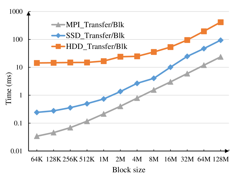
(a) Data Transfer Time via MPI, SSD and HDD

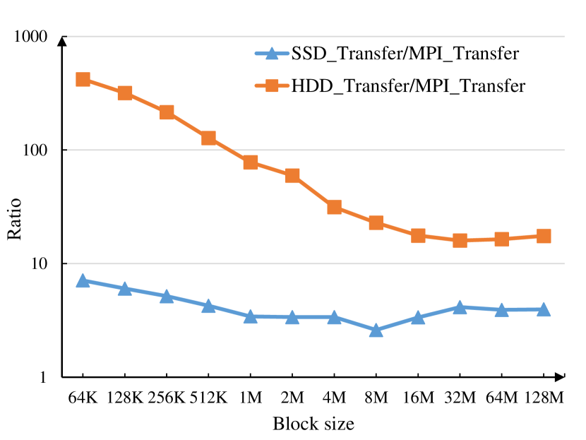
(b) Ratio of MPI/SSD and MPI/HDD

Figure 3: Data transfer Time and speedup for one block data on Comet.

From the above experiment results, we can summarize that MPI message is good at transferring small data size, but its performance drops when transferring larger data size. Moreover, on both machines, we find that MPI renders at most 19 times better performance when block size increases to 128MB. Thus, parallel file system is not that slow in the case of transferring large file. Especially when equipped with SSD, file system will be helpful in transferring both small and large data size.

4 Analytical modelling based end-to-end time optimization

1 The Problem

This chapter targets an important class of scientific discovery applications which require combining extreme-scale computational modeling/simulation with large-scale data analysis. The scientific discovery consists of computation, result output, result input, and data analysis. From a user’s perspective, the actual time-to-solution is the end-to-end time from the start of the computation to the end of the analysis. While it seems to be a simple problem with only four steps, different methods to execute the four steps can lead to totally different execution time. For instance, traditional methods execute the four steps sequentially such that the overall time-to-solution is the sum of the four times.

In this section, we study how to unify the four seemingly separated steps into a single problem and build an analytical model to analyze and predict how to obtain optimized time-to-solution. The rest of the section models the time-to-solution for three different methods: 1) the traditional method, 2) an improved version of the traditional method, and 3) the fully asynchronous pipeline method.

2 The Traditional Method

Figure 4 illustrates the traditional method, which is the simplest method without optimizations (next subsection will show an optimized version of the traditional method) [8]. The traditional method works as follows: the compute processes compute results and write computed results to disks, followed by the analysis processes reading results and then analyzing the results.

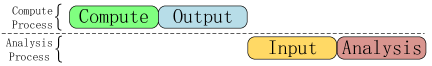
Figure 4: The traditional method.

The time-to-solution ($t2s$) of the traditional method can be expressed as follows:

$$T_{t2s}=T_{comp}+T_{o}+T_{i}+T_{analy}$$

,where $T_{comp}$ denotes the parallel computation time, $T_{o}$ denotes the output time, $T_{i}$ denotes the input time, and $T_{analy}$ denotes the parallel data analysis time. Although the traditional method can simplify the software development work, this formula reveals that the traditional model can be as slow as the accumulated time of all the four stages.

3 Improved Version of the Traditional Method

The traditional method is a strictly sequential workflow. However, it can be improved by using multi-threaded I/O libraries, where I/O threads are deployed to write results to disks meanwhile new results are generated by the compute processes. The other improvement is that the user input is divided into a number of fine-grain blocks and written to disks asynchronously. Figure 5 shows this improved version of the traditional method [8]. We can see that the output stage is now overlapped with the computation stage so that the output time might be hidden by the computation time.

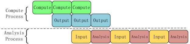
Figure 5: An improved version of the traditional method.

Suppose a number of $P$ CPU cores are used to compute simulations and a number of $Q$ CPU cores are used to analyze results, and the total amount of data generated is $D$. Given a fine-grain block of size $B$, there are $n_{b}=\frac{D}{B}$ blocks. Since scalable applications most often have good load balancing, we assume that each compute core computes $\frac{n_{b}}{P}$ blocks and each analysis core analyzes $\frac{n_{b}}{Q}$ blocks. The rationale behind the assumption of load balancing is that a large number of fine-grain parallel tasks (e.g., $n_{b}\gg P$) will most likely lead to an even workload distribution among a relatively small number of cores.

Our approach uses the time to compute and analyze individual blocks to estimate the time-to-solution of the improved traditional method. Let $t_{comp}$, $t_{o}$, $t_{i}$, and $t_{anal}$ denote the time to compute a block, write a block, read a block, and analyze a block, respectively. Then we can get the parallel computation time $T_{comp}=t_{comp}\times\frac{n_{b}}{P}$, the data output time $T_{o}=t_{o}\times\frac{n_{b}}{P}$, the data input time $T_{i}=t_{i}\times\frac{n_{b}}{Q}$, and the parallel analysis time $T_{analy}=t_{analy}\times\frac{n_{b}}{Q}$. The time-to-solution of the improved version is defined as follows:

$$T_{t2s}=\max(T_{comp},T_{o},T_{i}+T_{analy})$$

The term $T_{i}+T_{analy}$ is needed because the analysis process still reads data and then analyzes data in a sequence. Note that this sequential analysis step can be further parallelized, which results in a fully asynchronous pipeline execution model (see the following subsection).

4 The Fully Asynchronous Pipeline Method

The fully asynchronous pipeline method is designed to completely overlap computation, output, input, and analysis such that the time-to-solution is merely one component, which is either computation, data output, data input, or analysis. Note that the other three components will not be observable in the end-to-end time-to-solution. As shown in Figure 6, every data block goes through four steps: compute, output, input, and analysis [8]. Its corresponding time-to-solution can be expressed as follows:

$$T_{t2s} =\max(T_{comp},T_{o},T_{i},T_{analy})$$

$$=\max(t_{comp}\times\frac{n_{b}}{P},t_{o}\times\frac{n_{b}}{P},t_{i}\times\frac{n_{b}}{Q},t_{analy}\times\frac{n_{b}}{Q})$$

The above analytical model provides an insight into how to achieve an optimal time-to-solution. When $t_{comp}=t_{o}=t_{i}=t_{analy}$, the pipeline is able to proceed without any stalls and deliver the best performance possible. On the other hand, the model can be used to allocate and schedule computing resources to different stages appropriately to attain the optimal performance.

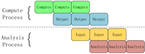
Figure 6: The fully asynchronous pipeline method.

5 Microbenchmark for the Analytical Model

To apply the analytical model in practice to predict the end-to-end time-to-solution, we need to know $t_{comp},t_{o},t_{i}$ and $t_{analy}$ on one block respectively. Given an application’s block size, users can get $t_{comp}$ and $t_{analy}$ simply by running their sequential kernel of computation and analysis on one block. The next step is to get $t_{o}$ and $t_{i}$.

At first, we design a naive microbenchmark to estimate $t_{o}$ and $t_{i}$. The microbenchmark contains $P$ writer threads and $Q$ reader threads. The mapping between writer threads and reader threads is static. Given a block size, each writer thread creates $n$ blocks filled with random values and writes them to disk. After all the $P$ writer threads have completed, the $Q$ reader threads start reading the files one by one. We measure the total time of writing files as $T_{o}$ and the total time of reading files as $T_{i}$ on each thread. Thus, we get $t_{o}=\frac{T_{o}}{n}$ and $t_{i}=\frac{T_{i}\times Q}{P\times n}$.

However, the above naive microbenchmark does not consider the scenario where multiple writes and reads can execute concurrently and asynchronously. Thus, we propose a new version microbenchmark. Figure 7 illustrates its idea, each writer thread will generate $n$ blocks in $m$ steps. Thus $k=\frac{n}{m}$ blocks are written into disk in each steps. Reader threads wait in the first step and start reading files in the second step, and then reads the blocks generated by the writers in the previous step.

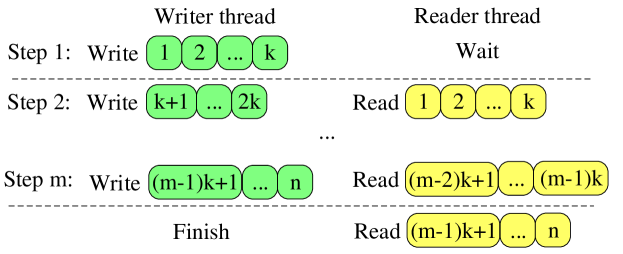
Figure 7: The Barrier Microbenchmark.

To achieve this idea, we use MPI_Barrier to synchronize between writer and reader threads. As shown in Algorithm 1 and 2, at the end of each step, all writers and readers will perform MPI_Barrier to control $k=n/m$ blocks to be written and read. With this approach, we can simulate the scenario that file writing and reading executed at the same time.

Algorithm 1 Writer thread in new microbenchmark

1:for $i=0$ to $m$ do

2:     $blk\_id\_begin=i*n/m$

3:     $blk\_id\_end=(i+1)*n/m$

4:     for $blk\_id=blk\_id\_begin$ to $blk\_id\_end$ do

5:         Write the block of $blk\_id$ to disk

6:     end for

7:     MPI_Barrier

8:end for

Algorithm 2 Reader thread in new microbenchmark

1:MPI_Barrier

2:for $i=1$ to $m$ do

3:     $blk\_id\_begin=(i-1)*n/m$

4:     $blk\_id\_end=i*n/m$

5:     for $blk\_id=blk\_id\_begin$ to $blk\_id\_end$ do

6:         Read the block of $blk\_id$ from the mapped writer processes

7:     end for

8:     if $i=m$ then break

9:     end if

10:     MPI_Barrier

11:end for

Then we perform experiments by different $P$ and $Q$ configurations on BigRed II. After we get the $t_{o}$ and $t_{i}$ from the two microbenchmarks, we compare them with the $t_{o}$ and $t_{i}$ obtained from the real application. At last, we use the relative error of writing and reading (i.e. $\frac{|{t_{Real\_app}-t_{Naive\_MB}}|}{t_{Real\_app}}$ and $\frac{|{t_{Real\_app}-t_{Barrier\_MB}}|}{t_{Real\_app}}$) to reflect the accuracy for each microbenchmark.

The results for two version of microbenchmark with 1 writer and 1 reader are displayed in Figure 8. For the writing relative error, the two versions of microbenchmark have similar accuracy among different block sizes. But for the reading relative error, the new microbenchmark gets better accuracy than naive version on all block sizes. The relative error of new microbenchmark is 20.5% on average among different block sizes, while 40.5% in naive version. In this case, the new one has similar accuracy on writing, but it has better accuracy on reading.

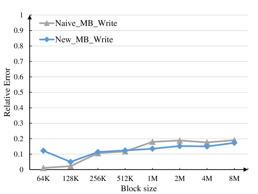
(a) $t_{o}$ Relative Error

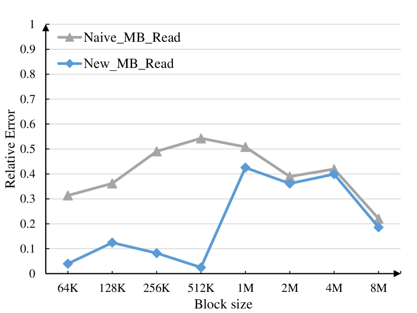
(b) $t_{i}$ Relative Error

Figure 8: Accuracy of two microbenchmark compared to Real Application with 1 writer and 1 reader on BigRed II.

Figure 9 shows the relative error on writing and reading with 4 writer threads and 1 reader thread. For the writing relative error, the new microbenchmark has better accuracy with 10% on average among different block sizes, while the naive microbenchmark has 12% on average. For the reading relative error, the new microbenchmark also obtains better accuracy with 19.5% on average among different block sizes, while the naive microbenchmark has 29% on average. Thus, the new version slightly outperforms naive version on writing, while has higher accuracy on reading.

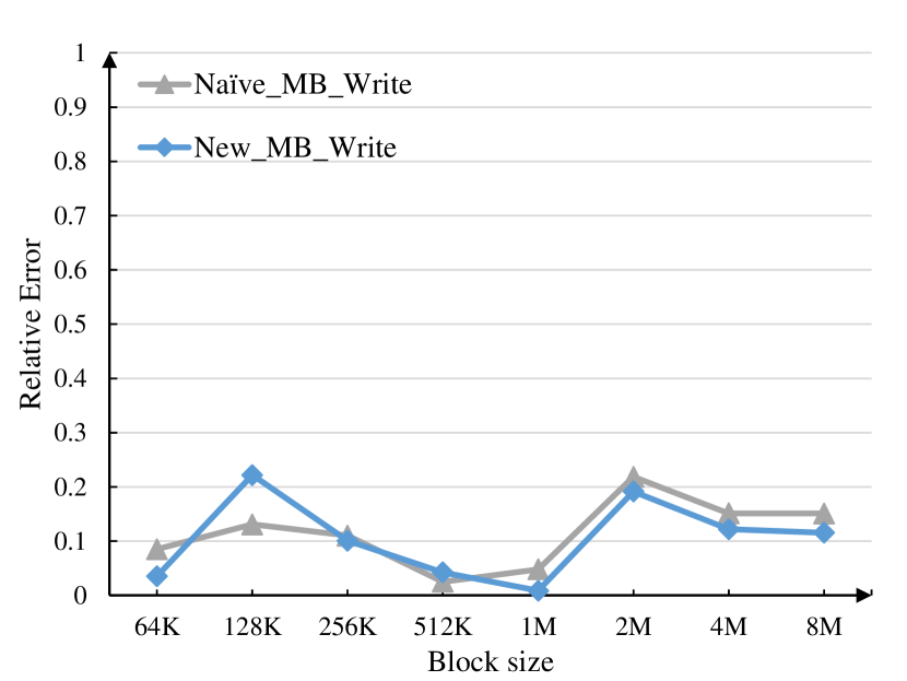
(a) $t_{o}$ Relative Error

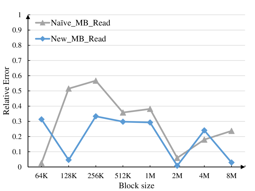
(b) $t_{i}$ Relative Error

Figure 9: Accuracy of the two microbenchmark compared to Real Application with 4 writers and 1 reader on BigRed II.

Figure 10 shows the relative error on writing and reading with 16 writer threads and 4 reader threads. For the writing relative error, the new microbenchmark has better accuracy with 9% on average among different block sizes, while the naive microbenchmark has 16% on average. For the reading relative error, the new microbenchmark also obtains better accuracy with 21% on average among different block sizes, while the naive microbenchmark has 24.6% on average. In this case, the new version outperforms naive version on both writing and reading accuracy.

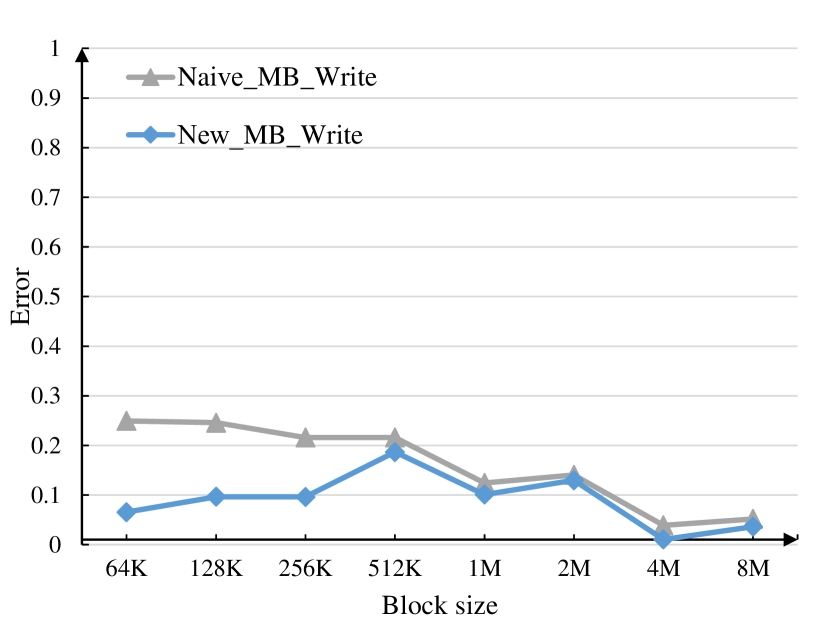
(a) $t_{o}$ Relative Error

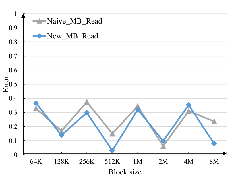
(b) $t_{i}$ Relative Error

Figure 10: Accuracy of two microbenchmark compared to Real Application with 16 writers and 4 readers on BigRed II.

Figure 11 shows the relative error on writing and reading with 16 writer threads and 4 reader threads. For the writing relative error, the new microbenchmark has better accuracy with 13.5% on average among different block sizes, while the naive microbenchmark has 23.4% on average. Besides, the naive version even gets a relative error up to 59% on 8MB. For the reading relative error, the new microbenchmark also obtains better accuracy with 27% on average among different block sizes, while the naive microbenchmark has 29% on average. Thus, in this case, the new version also outperforms the naive one on both writing and reading accuracy.

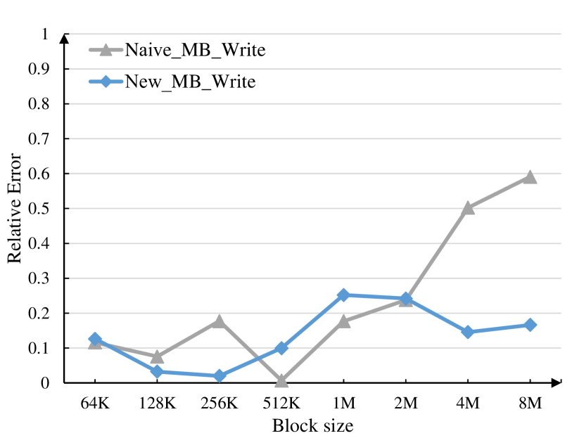
(a) $t_{o}$ Relative Error

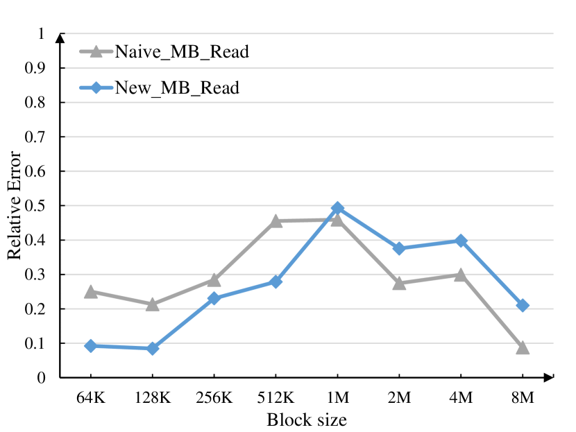
(b) $t_{i}$ Relative Error

Figure 11: Accuracy of two microbenchmark compared to Real Application with 32 writers and 32 readers on BigRed II.

From the above experiment results, we observe that the new microbenchmark never gets a relative error of more than 50%. Besides, it gets an average relative error rate up to 13.5% for writing and up to 25% for reading among all cases and different threads configuration. Thus, we can conclude that the new version is more accurate than the naive version. The reason that the microbenchmark can not sometimes predict the $t_{o}$ and $t_{i}$ accurately is that we do not consider network contention and sharing among the parallel file system between users into the microbenchmark model. And to add these two parts into the microbenchmark is not a trivial job and we do not expect the microbenchmark too complicated. But we still can use the microbenchmark to get the trends and acceptable I/O performance to predict $t_{o}$ and $t_{i}$ in real applications.

5 Design and Implementation of DataBroker for the Fully Asynchronous Method

To enable the fully asynchronous pipeline model, we design and develop a software prototype called Intelligent DataBroker. The interface of the DataBroker prototype is similar to Unix’s pipe, which has a writing end and a reading end. For instance, a computation process will call DataBroker.write(block_id, void* data) to output data, while an analysis process will call DataBroker.read(block_id) to input data. Although the interface is simple, it has its own runtime system to provide pipelining, hierarchical buffering, and data prefetching.

Figure 12 shows the design of DataBroker [8]. It consists of two components: a DataBroker producer component in the compute node to send data, and a DataBroker consumer component in the analysis node to receive data. The producer component owns a producer ring buffer and one or multiple producer threads to process output in parallel. Each producer thread looks up the I/O-task queues and uses priority-based scheduling algorithms to transfer data to destinations in a streaming manner. A computational process may send data to an analysis process via two possible paths: message passing by the network, or file I/O by the parallel file system. Depending on the execution environment, it is possible that both paths are available and used to speed up the data transmission time.

The DataBroker consumer is co-located with an analysis process on the analysis node. The consumer component will receive data from the computation processes, buffer data, and prefetch and prepare data for the analysis application. It consists of a consumer ring buffer and one or multiple prefetching threads. The prefetching threads are responsible for making sure there are always data blocks available in memory by loading blocks from disks to memory. Since we assume a streaming-based data analysis, the prefetching method can use the technique of read ahead to prefetch data efficiently.

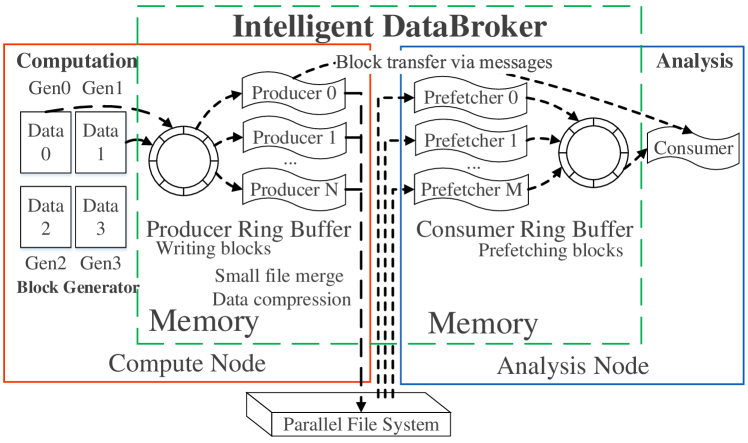
Figure 12: Architecture of the DataBroker middleware for coupling computation with analysis in a streaming pipeline manner. DataBroker consists of a producer component on a compute node, and a consumer component on an analysis node.

6 Experiments with Synthetic and Real Applications

We perform experiments to verify the accuracy of the analytical model and to evaluate the performance of the fully asynchronous pipeline method, respectively. For each experiment, we collect performance data from two different programs: 1) a synthetic application, and 2) a real-world computational fluid dynamics (CFD) application. All the experiments are carried out on BigRed II (a Cray XE6/XK7 system) configured with the Lustre 2.1.6 distributed parallel file system at Indiana University. Every compute node on BigRed II has two AMD Opteron 16-core Abu Dhabi CPUs and 64 GB of memory, and is connected to the file system via 56-Gb FDR InfiniBand which is also connected to the DataDirect Network SFA12K storage controllers.

1 Synthetic and Real-World Applications

The synthetic application consists of a computation stage and an analysis stage. To perform these experiments, we use 32 compute nodes to execute the computation stage, and use two different numbers of analysis nodes (i.e., 2 analysis nodes and 32 analysis nodes) to execute the analysis stage, respectively. We launch one process per node. Each computation process randomly generates a total amount of 1GB data (chopped to small blocks) and writes the data to the DataBroker producer. Essentially, the computation processes only generate data, but not perform any computation. At the same time, each analysis process reads data from its local DataBroker consumer and computes the sum of the square root of the received data block for a number of iterations. The mapping between computation processes and analysis processes is static. For instance, if there are 32 computation processes and 2 analysis processes, each analysis process will process data from a half of the computation processes.

Our real-world CFD application, provided by the Mathematics Department at IUPUI [22], computes the 3D simulations of flow slid of viscous incompressible fluid flow at 3D hydrophobic microchannel walls using the lattice Boltzmann method [9, 15]. This application is written in ANSI C and MPI. We replaced all the file write functions in the CFD application by our DataBroker API. The CFD simulation is coupled with an data analysis stage, which computes a series of statistical analysis functions at each fluid region for every time step of the simulation. Our experiment takes as input a 3D grid of $512\times 512\times 256$, which is distributed to different computation processes. Similar to the synthetic experiments, we also run 32 computation processes on 32 compute nodes while running different numbers of analysis processes. For each experiment, we execute it four times and display their average in our experimental results.

2 Accuracy of the Analytical Model

We experiment with both the synthetic application and the CFD application to verify the analytical model. Our experiments measure the end-to-end time-to-solution on different block sizes ranging from 128KB to 8MB. The experiments are designed to compare the time-to-solution estimated by the analytical model with the actual time-to-solution to show the model’s accuracy.

Figure 13 (a) shows the actual time and the predicted time of the synthetic application using 32 compute nodes and 2 analysis nodes [8]. For all different block sizes, the analysis stage is the largest bottleneck among the four stages (i.e., computation, output, input, and analysis). Hence, the time-to-solution is essentially equal to the analysis time. Also, the relative error between the predicted and the actual execution time is from 1.1% to 12.2%, and on average 3.9%. Figure 13 (b) shows the actual time and the predicted time for the CFD application [8]. Different from the synthetic application, its time-to-solution is initially dominated by the input time when the block size is 128KB, then it becomes dominated by the analysis time from 256KB to 8MB. The relative error of the analytical model is between 4.7% and 18.1%, and on average 9.6%.

The relative error is greater than zero because our analytical model ignores the pipeline startup and drainage time, and there is also a small amount of pipeline idle time and jitter time during the real execution. Please note that each analysis process has to process the computed results from 16 computation processes.

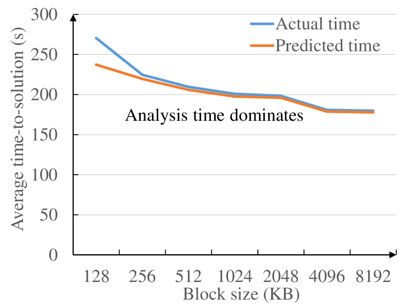
(a) Synthetic experiments

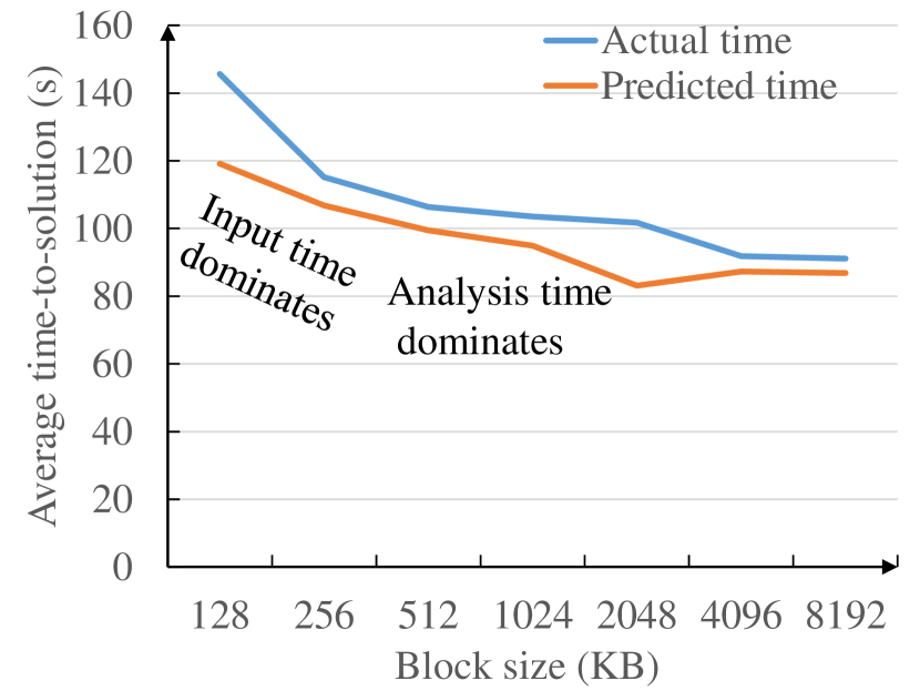
(b) CFD application

Figure 13: Accuracy of the analytical model for the fully asynchronous pipeline execution with 32 compute nodes and 2 analysis nodes.

Figure 14 (a) shows the performance of the synthetic application that uses 32 compute nodes and 32 analysis nodes [8]. When the block size is equal to 128KB, the input time dominates the time-to-solution. When the block size is greater than 128KB, the data analysis time starts to dominate the time-to-solution. The turning point in the figure also verifies the bottleneck switch (from the input stage to the analysis stage). The predicted time and the actual time are very close to each other and have an average relative error of 9.1%. Similarly, Figure 14 (b) shows an relative error of 0.9% for the CFD application that also uses 32 compute nodes and 32 analysis nodes [8].

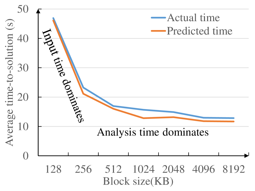
(a) Synthetic experiments

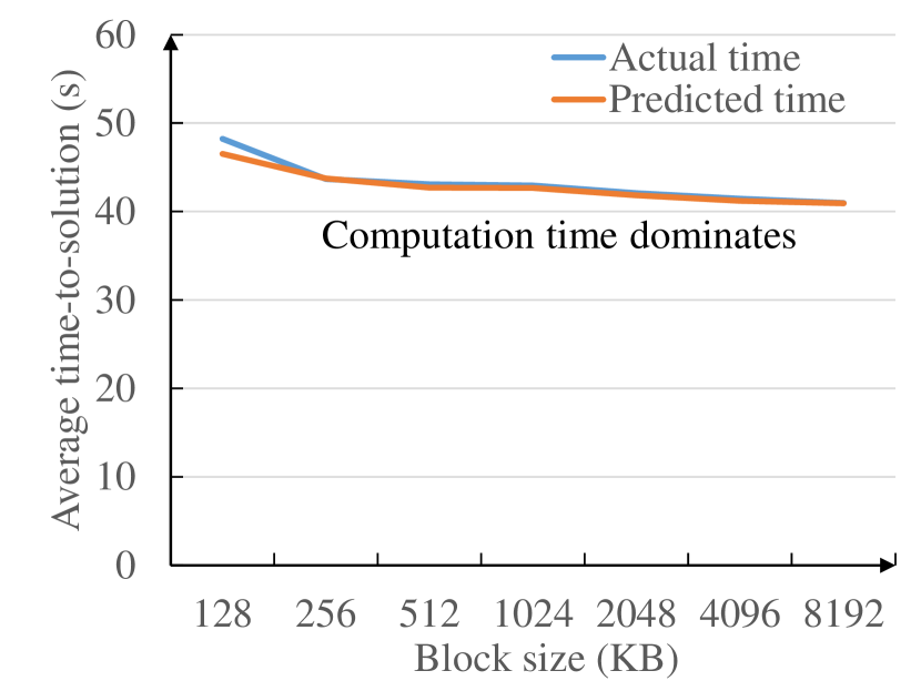
(b) CFD application

Figure 14: Accuracy of the analytical model for the fully asynchronous pipeline execution with 32 compute nodes and 32 analysis nodes.

3 Performance Speedup

Besides testing the analytical model, we also conduct experiments to evaluate the performance improvement by using the fully asynchronous pipeline method. The experiments compare three different approaches (i.e., three implementations) to executing the integrated computation and analysis: 1) the traditional method, 2) the improved version of the traditional method which builds upon fine-grain blocks and overlaps computation with data output, and 3) the fully asynchronous pipeline method based on DataBroker. Each of the three implementations takes the same input size and is compared with each other in terms of wall clock time.

Figure 15 (a) and (b) show the speedup of the synthetic application and the real-world CFD application, respectively [8]. Note that the baseline program is the traditional method (i.e., speedup=1). The data in Figure 15 (a) shows that the improved version of the traditional method can be up to 18 times faster than the traditional method when the block size is equal to 8MB [8]. It seems to be surprising, but by looking into the collected performance data, we discover that reading two 16GB files by two MPI process simultaneously is 59 times slower than reading a collection of small 8MB files by the same two MPI processes. This might be because two 16GB files are allocated to the same storage device, while a number of 8MB files are distributed to multiple storage devices. On the other hand, the fully asynchronous pipeline method is faster than the improved traditional method by up to 131% when the block size is equal to 128KB. Figure 15 (b) shows the speedup of the CFD application [8]. We can see that the fully asynchronous method is always faster (up to 56%) than the traditional method whenever the block size is larger than 128KB. The small block size of 128KB does not lead to improved performance because writing small files to disks can incur significant file system overhead and cannot reach the maximum network and I/O bandwidth. Also, the fully asynchronous method is consistently faster than the improved traditional method by 17% to 78%.

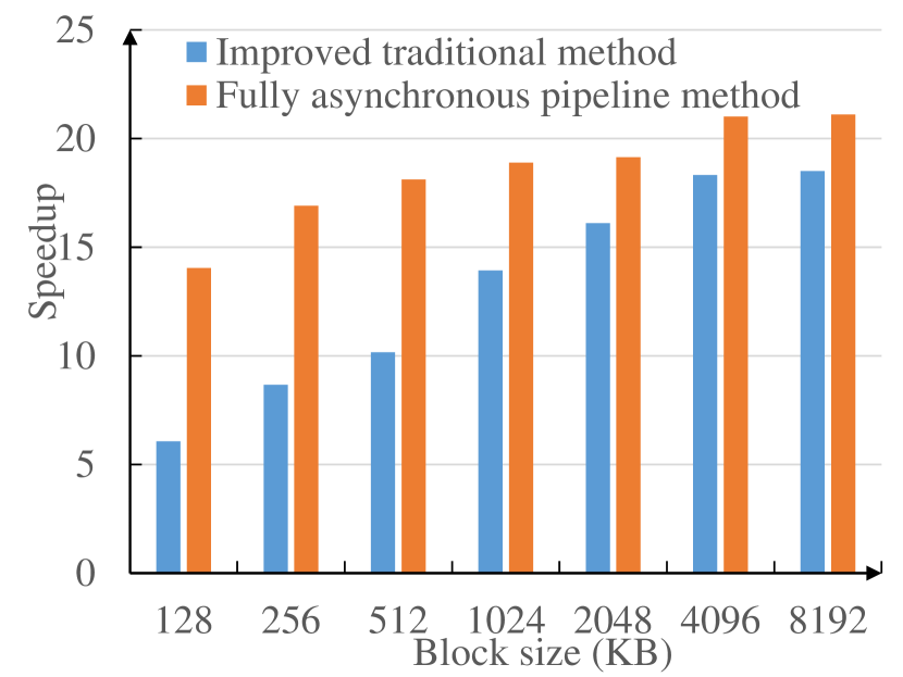
(a) Synthetic experiments

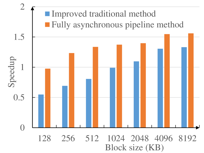
(b) CFD application

Figure 15: Performance comparison between the traditional, the improved, and the DataBroker-based fully asynchronous methods using 32 compute nodes and 2 analysis nodes.

Figure 16 (a) shows the speedup of the synthetic application that uses 32 compute nodes and 32 analysis nodes [8]. We can see that the fully asynchronous pipeline method is 49% faster than the traditional method when the block size is equal to 8MB. It is also 24% faster than the improved transitional method when the block size is equal to 4MB. Figure 16 (b) shows the speedup of the CFD application with 32 compute nodes and 32 analysis nodes [8]. Both the fully asynchronous pipeline method and the improved traditional method are faster than the traditional method. For instance, they are 31% faster with the block size of 8MB. However, the fully asynchronous pipeline method is almost the same as the improved method when the block size is bigger than 128KB. This is because the specific experiment’s computation time dominates its time-to-solution so that both methods’ time-to-solution is equal to the computation time, which matches our analytical model.

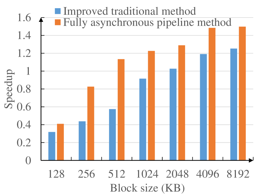
(a) Synthetic experiments

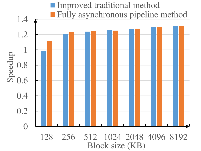
(b) CFD application

Figure 16: Performance comparison between the traditional, the improved, and the DataBroker-based fully asynchronous methods using 32 compute nodes and 32 analysis nodes.

7 Open Issues and Challenges

This chapter presents a new way to accelerate scientific workflows consisting of computation-intensive applications and data-intensive applications. Although the current method has shown promising results, there are more open issues and challenging problems. Here we provide a list of challenging problems as follows:

• Is it possible to design an adaptive data transfer method that can utilize both message passing and parallel file systems concurrently at runtime? Considering new file systems will utilize more Nonvolatile Memories (NVM), the performance difference between memory and file system becomes lesser.

• How to utilize the proposed analytical model to schedule computing resources more efficiently? It can lead to more efficient scheduling methods.

• Is it possible to extend the task-based pipeline approach to a general workflow model that consists of applications in a task graph?

• How to build a general-purpose workflow framework and programming tool to automatically combine different applications seamlessly at the fine-grain task level?

These open issues and challenges will require further research in SDN to facilitate faster data transfer and minimized time-to-solution in tightly coupled workflow applications.

8 Conclusion

To facilitate the convergence of computational modeling/simulation and the big data analysis, in this chapter we study the problem of integrating computation with analysis in both theoretical and practical ways. First, we use the metric of the time-to-solution of scientific discovery to formulate the integration problem and propose a fully asynchronous pipeline method to model the execution. Next, we build an analytical model to estimate the overall time to execute the asynchronous combination of computation and analysis. In addition to the theoretical foundation, we also design and develop an intelligent DataBroker to help fully interleave the computation stage and the analysis stage.

The experimental results show that the analytical model can estimate the time-to-solution with an average relative error of less than 10%. By applying the fully asynchronous pipeline model to both synthetic and real-world CFD applications, we can increase the performance of the improved traditional method by up to 131% for the synthetic application, and up to 78% for the CFD application.

Acknowledgements

This material is based upon research partially supported by the Purdue Research Foundation and by the NSF Grant No. 1522554. Development and experiment of the software framework have used the NSF Extreme Science and Engineering Discovery Environment (XSEDE), which is supported by National Science Foundation grant number ACI-1053575.

References

- [1] H. Abbasi, J. Lofstead, F. Zheng, K. Schwan, M. Wolf, and S. Klasky. Extending I/O through high performance data services. In IEEE International Conference on Cluster Computing and Workshops (CLUSTER’09), pages 1–10. IEEE, 2009.
- [2] H. Abbasi, M. Wolf, G. Eisenhauer, S. Klasky, K. Schwan, and F. Zheng. Datastager: Scalable data staging services for petascale applications. Cluster Computing, 13(3):277–290, 2010.
- [3] G. Aloisioa, S. Fiorea, I. Foster, and D. Williams. Scientific big data analytics challenges at large scale. Proceedings of Big Data and Extreme-scale Computing, 2013.
- [4] J. Bent, G. Gibson, G. Grider, B. McClelland, P. Nowoczynski, J. Nunez, M. Polte, and M. Wingate. PLFS: A checkpoint filesystem for parallel applications. In Proceedings of the Conference on High Performance Computing Networking, Storage and Analysis (SC’09), page 21. ACM, 2009.
- [5] J. Chen, A. Choudhary, S. Feldman, B. Hendrickson, C. Johnson, R. Mount, V. Sarkar, V. White, and D. Williams. Synergistic challenges in data-intensive science and exascale computing. DOE ASCAC Data Subcommittee Report, Department of Energy Office of Science, 2013.
- [6] J. Dayal, J. Cao, G. Eisenhauer, K. Schwan, M. Wolf, F. Zheng, H. Abbasi, S. Klasky, N. Podhorszki, and J. Lofstead. I/O Containers: Managing the data analytics and visualization pipelines of high end codes. In Proceedings of the 2013 IEEE 27th International Symposium on Parallel and Distributed Processing Workshops and PhD Forum, IPDPSW ’13, pages 2015–2024, Washington, DC, USA, 2013. IEEE Computer Society.
- [7] C. Docan, M. Parashar, and S. Klasky. DataSpaces: An interaction and coordination framework for coupled simulation workflows. Cluster Computing, 15(2):163–181, 2012.
- [8] Y. Fu, F. Song, and L. Zhu. Modeling and implementation of an asynchronous approach to integrating hpc and big data analysis. Procedia Computer Science, pages 52–62, 2016.
- [9] Z. Guo and C. Shu. Lattice Boltzmann method and its applications in engineering. World Scientific, 2013.
- [10] H. Huang and L. L. Knowles. Unforeseen consequences of excluding missing data from next-generation sequences: Simulation study of RAD sequences. Systematic biology, pages 1–9, 2014.
- [11] Q. Liu, J. Logan, Y. Tian, H. Abbasi, N. Podhorszki, J. Y. Choi, S. Klasky, R. Tchoua, J. Lofstead, and R. Oldfield. Hello ADIOS: The challenges and lessons of developing leadership class I/O frameworks. Concurrency and Computation: Practice and Experience, 26(7):1453–1473, 2014.
- [12] J. Lofstead, R. Oldfield, T. Kordenbrock, and C. Reiss. Extending scalability of collective IO through Nessie and staging. In Proceedings of the sixth workshop on Parallel Data Storage, pages 7–12. ACM, 2011.
- [13] K.-L. Ma. In situ visualization at extreme scale: Challenges and opportunities. Computer Graphics and Applications, IEEE, 29(6):14–19, 2009.
- [14] S. Madadgar, H. Moradkhani, and D. Garen. Towards improved post-processing of hydrologic forecast ensembles. Hydrological Processes, 28(1):104–122, 2014.
- [15] P. Nagar, F. Song, L. Zhu, and L. Lin. LBM-IB: A parallel library to solve 3D fluid-structure interaction problems on manycore systems. In Proceedings of the 2015 International Conference on Parallel Processing, ICPP’15. IEEE, September 2015.
- [16] D. A. Patterson and J. L. Hennessy. Computer organization and design: the hardware/software interface. Newnes, 2013.
- [17] A. B. Shiflet and G. W. Shiflet. Introduction to computational science: Modeling and simulation for the sciences. Princeton University Press, 2014.
- [18] R. Thakur, W. Gropp, and E. Lusk. On implementing MPI-IO portably and with high performance. In Proceedings of the sixth workshop on I/O in parallel and distributed systems, pages 23–32. ACM, 1999.
- [19] V. Vishwanath, M. Hereld, M. E. Papka, R. Hudson, G. C. Jordan IV, and C. Daley. In situ data analysis and I/O acceleration of FLASH astrophysics simulation on leadership-class system using GLEAN. In Proc. SciDAC, Journal of Physics: Conference Series, 2011.
- [20] P. C. Wong, H.-W. Shen, C. R. Johnson, C. Chen, and R. B. Ross. The top 10 challenges in extreme-scale visual analytics. IEEE computer graphics and applications, 32(4):63, 2012.
- [21] F. Zheng, H. Zou, G. Eisenhauer, K. Schwan, M. Wolf, J. Dayal, T.-A. Nguyen, J. Cao, H. Abbasi, and S. Klasky. FlexIO: I/O middleware for location-flexible scientific data analytics. In IEEE 27th International Symposium on Parallel & Distributed Processing (IPDPS), pages 320–331. IEEE, 2013.
- [22] L. Zhu, D. Tretheway, L. Petzold, and C. Meinhart. Simulation of fluid slip at 3D hydrophobic microchannel walls by the lattice Boltzmann method. Journal of Computational Physics, 202(1):181–195, 2005.