An automatic procedure to determine groups of nonparametric regression curves

Abstract

In many situations it could be interesting to ascertain whether nonparametric regression curves can be grouped, especially when confronted with a considerable number of curves. The proposed testing procedure allows to determine groups with an automatic selection of their number. A simulation study is presented in order to investigate the finite sample properties of the proposed methods when compared to existing alternative procedures. Finally, the applicability of the procedure to study the geometry of a tunnel by analysing a set of cross-sections is demonstrated. The results obtained show the existence of some heterogeneity in the tunnel geometry.

Keywords multiple regression curves  $\cdot$ nonparametric regression  $\cdot$ testing equality  $\cdot$ number of groups  $\cdot$ clustering  $\cdot$ tunnel profile

1 Introduction

One of the main goals of statistical modelling is to understand the dependence of a response variable, $Y$, with respect to another explanatory variable, $X$. This type of dependence can be studied through nonparametric regression models, where the relationship between $Y$ and $X$ is modelled without specifying in advance the function that links them. Within this framework, the study of the regression curves can be useful in the comparison of two or more groups, which is an important problem associated with statistical inference. In particular, the topic of hypothesis testing the equality of mean functions has been widely investigated in the literature, see, for instance, the review that González-Manteiga and Crujeiras (2013) offers about this topic. Relevant papers on this topic are Hall and Hart (1990); King et al. (1991); Delgado (1993); Kulasekera (1995); Young and Bowman (1995); Dette and Neumeyer (2001); Pardo-Fernández et al. (2007); Srihera and Stute (2010), among others. Furthermore, in order to compare the values of a response variable across several groups in the presence of a covariate effect, nonparametric analysis of covariance or factor-by-curve interaction test can be used. Young and Bowman (1995) generalized the one-way analysis of variance test to the nonparametric regression setting, and Dette and Neumeyer (2001) proposed to use Young and Bowman’s test also in the situation of a heteroscedastic error. In addition, Park and Kang (2008) developed a SiZer tool based on an analysis of variance type test statistic that is capable of comparing multiple curves based on the residuals. The evolution of this procedure is based on the comparison using the original regression curves (Park et al., 2014). More recently, the possibility of comparing curves as well as their derivatives has been proposed by Sestelo and Roca-Pardiñas (2019) using factor-by-curve interactions in a nonparametric framework.

When the null hypothesis of equality of curves is rejected, leading to the clear conclusion that at least one curve is different, it can be interesting to ascertain whether groups of curves can exist or, by contrast, that all these curves are different from each other. In this setting, one naïve approach would be to perform pairwise comparisons. Following the ideas of Rosenblatt (1975); González-Manteiga and Cao (1993); Härdle and Mammen (1993b), an alternative test to check the null hypothesis of equality of curves obtained from a pairwise comparison of the estimators of the regression functions was proposed by Dette and Neumeyer (2001). A similar statistic was considered by King et al. (1991). However, such approaches lead to difficult interpretation of results because as the number of curves increases so does the number of comparisons. For example, considering 50 curves, the number of all pairwise comparisons that need to be conducted is 1225. One could make it but without the possibility of determining groups with similar regression curves.

With this focus but in time-to-event framework, Villanueva et al. (2019) have described a new procedure to determine groups in multiple survival curves. Some approaches have been developed also in functional data context (Abraham et al., 2003; García-Escudero and Gordaliza, 2005; Tarpey, 2007) and in longitudinal one (Vogt and Linton, 2017, 2020). However, to the best of our knowledge the problem of determining groups of regression functions in a standard nonparametric framework (cross-sectional data) has not been considered explicitly in the literature.

Based on the above, and taking into account situations with a considerable number of curves, we introduce an approach that allows us to group multiple regression curves. Briefly, our procedure is described as follows. Firstly, the $J$ regression curves are estimated by kernel smoothers. Secondly, given a number of $K$ groups, the optimal possible assignment of $J$ curves into $K$ groups is chosen by means of a heuristic algorithm. Finally, the optimal number of groups is determined using an automatic bootstrap-based testing procedure.

The proposed methodology is used to study the geometry of a tunnel by analysing a set of cross-sections along it. These sections were obtained by adjusting a surface to a point cloud measured with a terrestrial laser scanning. The existence of different groups of cross-sections indicates that the tunnel has a heterogeneous geometry. This heterogeneity could be due to bad construction or to deformations in the tunnel.

The remainder of this paper is organized as follows. In Section 2.1, the notation and the methodological background are explained. In Section 3, the performance of our and existing procedures is shown through simulation studies. The results of the analysis of a real dataset are provided in Section 4. Finally, the main conclusions of this work are exposed in Section 5.

2 Methodology

2.1 Notation and technical details

Let $(X_{j},Y_{j})$ be $J$ independent random vectors, and assume that they satisfy the following nonparametric regression models, for $j=1,\ldots,J$,

$$Y_{j}=m_{j}(X_{j})+\varepsilon_{j}$$ (1)

where $m_{j}$ is a nonparametric smooth function and $\varepsilon_{j}$ is the regression error, which is assumed independent of the covariate $X_{j}$. Note that, by construction, $E(\varepsilon_{j})=0$ and $Var(\varepsilon_{j})=\sigma_{j}^{2}$, which means that $m_{j}(X_{j})$ represents the conditional mean, while $\sigma_{j}^{2}$ equals the residuals variance, i.e., $\sigma_{j}^{2}=Var(Y_{j}-m_{j}(X_{j}))$. Throughout this paper, we will not require any assumptions on the error distributions.

Several approaches can be used to estimated the regression models in (1), such as, methods based on regression splines (de Boor, 2001), Bayesian approaches (Lang and Brezger, 2004) or local polynomial kernel smoothers (Wand and Jones, 1995; Fan and Gijbels, 1996). In this work, local linear kernel smoothers, as implemented in the npregfast R package (Sestelo et al., 2016, 2017), are used. Explicitly, given $J$ independent random samples, say

$$\left\{{S_{1}=\left\{{\left({X_{i1},Y_{i1}}\right)}\right\}_{i=1}^{n_{1}},\ldots,S_{J}=\left\{{\left({X_{iJ},Y_{iJ}}\right)}\right\}_{i=1}^{n_{J}}}\right\}$$

where the random variables $(X_{1j},Y_{1j}),\ldots,(X_{n_{j}j},Y_{n_{j}j})$ are i.i.d. for each $j=1,\ldots,J$ and with a total sample size $n=\sum_{j=1}^{J}n_{j}$, the local linear kernel estimator

$$\hat{m}_{j}(x)=\Psi(x,S_{j},h_{j})$$ (2)

at a location $x$ is given by $\hat{m}_{j}(x)=\hat{\alpha}_{0j}(x)$, where $\hat{\alpha}_{0j}(x)$ is the first element of the vector $(\hat{\alpha}_{0j}(x),\hat{\alpha}_{1j}(x))$ which is the minimiser of

$$\sum_{i=1}^{n_{j}}\left\{{Y_{ij}-\alpha_{0j}(x)-\alpha_{1j}(x)(X_{ij}-x)}\right\}^{2}\cdot\kappa\left({{\frac{{X_{ij}-x}}{h_{j}}}}\right),$$ (3)

where $\kappa$ denotes a kernel function (normally, a symmetric density), and $h_{j}>0$ is the smoothing parameter or bandwidth. Taking into account that nonparametric estimates depend heavily on the bandwidth $h_{j}$, various methods for an optimal selection have been suggested, such as Generalised Cross-Validation (Golub et al., 1979) or plug-in methods, see e.g., Ruppert et al. (1995). See Wand and Jones (1995) for a good overview of this topic. However, optimal bandwidth selection is still a challenging problem. As a practical solution, and based on the simulation results, the bandwidths $h_{j}$ can be selected automatically by minimising the following cross-validation criterion

$$CV(h_{j})={\sum\nolimits_{i=1}^{n_{j}}{\left({{Y}_{ij}-\hat{m}_{j}^{-i}(X_{ij})}\right)}}^{2},$$ (4)

where $\hat{m}_{j}^{-i}(X_{ij})$ indicates the fit at $X_{ij}$ leaving out the $i$-th data point based on the smoothing parameter $h_{j}$.

Additionally, it is well-known that bootstrap resampling techniques are time-consuming processes because the estimation of the model is carried out many times. Moreover, the use of cross-validation for selecting the bandwidth implies a high computational cost because it is necessary to repeat the estimation procedure several times to select the optimal estimate. Accordingly, to apply some computational acceleration technique is fundamental to ensure that the problem can be addressed adequately in practical situations. Thus, in this paper we use binning techniques to speed up the process. A detailed explanation of this technique can be found in Fan and Marron (1994).

2.2 The algorithm for determining groups

As pointed out in the Introduction, several nonparametric methods have been proposed in the literature in order to test the equality of regression curves, i.e., to test the null hypothesis $H_{0}:m_{1}=\ldots=m_{J}$. If the test is statistical significant and this hypothesis is thus rejected, then determining groups of regression curves becomes of interest, that is, assessing if the levels $\{1,\ldots,J\}$ can be grouped in $K$ groups $G_{1},\ldots,G_{K}$ with $K<J$ such that for each $k=1,\ldots,K$, $m_{i}=m_{j}$ for all $i,j\in G_{k}$. Note that $(G_{1},\ldots,G_{K})$ must be a partition of $\{1,\ldots,J\}$, and therefore must satisfy $G_{1}\cup\ldots\cup G_{K}=\{1,\ldots,J\}$ and $C_{i}\cap G_{j}=\emptyset$, for all $i\neq j\in\{1,\ldots,K\}$.

Let $(X_{ij},Y_{ij})$, $i=1,\ldots,n_{j}$, be an i.i.d. sample from the distribution of $(X_{j},Y_{j})$, for each $j=1,\ldots,J$, and with the total sample size $n=\sum_{j=1}^{J}n_{j}$, we propose a procedure to test, for a given a number $K$, the null hypothesis $H_{0}(K)$ that at least one partition exists $(G_{1},\ldots,G_{K})$ so that all the conditions above are satisfied. The alternative hypothesis $H_{1}(K)$ is that for any $(G_{1},\ldots,G_{K})$, exists at least a group $G_{k}$ in which $m_{i}\neq m_{j}$ for some $i,j\in G_{k}$.

The testing procedure is based on the $J$-dimensional process

$${\bf{\widehat{V}}}(z)=(\widehat{V}_{1}(z),\widehat{V}_{2}(z),\ldots,\widehat{V}_{J}(z))^{t},$$

where, for $j=1,\ldots,J$,

$$\widehat{V}_{j}(z)=\sum_{k=1}^{K}[\widehat{m}_{j}(z)-\widehat{f}_{k}(z)]\hskip 2.84544ptI_{\{j\in G_{k}\}}$$

and $\widehat{f}_{k}$ is the pooled local linear kernel estimate based on the combined $G_{k}$-partition sample, i.e.,

$$\widehat{f}_{k}(z)=\Psi(z,S_{k},h_{k})$$

where

$$S_{k}=\sum_{j\in G_{k}}S_{j}.$$

The following test statistics were considered in order to test $H_{0}(K)$: a Cramér-von Mises type test statistic

$$D_{CM}=\min\limits_{G_{1},\ldots,G_{K}}\quad\sum\limits_{j=1}^{J}\int_{R_{X}}{\widehat{V}^{2}_{j}(z)}dz$$

and a modification of it based on the $L_{1}$ norm proposed in the Kolmogorov-Smirnov test statistic

$$D_{KS}=\min\limits_{G_{1},\ldots,G_{K}}\quad\sum\limits_{j=1}^{J}\int_{R_{X}}{|\widehat{V}_{j}(z)|}dz$$

In order to solve the minimisation problem in each test statistic, all the different assignments of the $J$ curves into $K$ groups have to be evaluated. Because of the large number of calculations, this method is feasible only for small numbers of $J$ and $K$. Obviously, when confronted with a large number of $J$ curves, the procedure requires an excessively high computational cost. To be more specific, we deal in our study of tunnel cross-sections with $J=66$ curves and $K=5$ groups and, taking into account the formula of Jain and Dubes (1988), the total number of different assignments is 1e44. This combinatorial explosion implies that the problem becomes intractable. Therefore, heuristic algorithms would be really appropriate to tackle much bigger problems. One the one hand, in the case of $D_{CM}$ test statistic which is defined in terms of the $L_{2}$-distance, we propose the use of the $K$-means (Macqueen, 1967). On the other hand, for the $D_{KS}$ test statistic defined in terms of the $L_{1}$-norm, the $K$-medians (Macqueen, 1967; Kaufman and Rousseeuw, 1990) would be more suitable. In both cases, the carried out procedure is equivalent: the regression functions $m_{j}$ ($j=1,\ldots,J$) have to be estimated in a common grid of size $Q$ leading to a matrix of ($J$ x $Q$) dimension, where each row corresponds with the estimates of the $j$ curve in the $Q$ positions of the grid. Then, this matrix will be the input of both heuristic methods, $K$-means and $K$-medians, and from these the “best” partition ($G_{1},\ldots,G_{K}$) is obtained.

Finally, the decision rule based on $D$ consists of rejecting the null hypothesis if $D$ is larger than $(1-\alpha)$-percentile obtained under the null hypothesis. To approximate the distributions of the test statistics, resampling methods such as the bootstrap introduced by Efron (1979) (see also Efron and Tibshirani (1993); Härdle and Mammen (1993a); Kauermann and Opsomer (2003)) can be applied instead. Here we use the wild bootstrap (Wu, 1986; Liu, 1988; Mammen, 1993) because this method is valid both for homoscedastic and for heteroscedastic models where the variance of the error is a function of the covariate.

The testing procedure used requires the following steps:

Step 1. Using the original sample, for $j=1,\ldots,J$ and $i=1,\ldots,n_{j}$, estimate in a common grid the regression functions $m_{j}$, using each sample separately. Then, applying the proposed algorithms, obtain the “best” partition ($G_{1},\ldots,G_{K}$) and with it, obtain the estimated curves $\widehat{f}_{k}$ using a pooled local linear kernel estimator based on the combined partition samples.

Step 2. Obtain the $D$ value as explained before, and the null errors under the $H_{0}(k)$ as

$$\widehat{\varepsilon}_{ij}=\sum_{k=1}^{K}\left({Y_{ij}-\widehat{f}_{k}(X_{ij})}\right)I_{\{j\in G_{k}\}}.$$

Step 3. Draw bootstrap samples as follows, for $b=1,\ldots,B$, and for each $j\in G_{k}$,
draw $\left\{{\left({X_{i1},Y_{i1}^{\ast b}}\right)}\right\}_{i=1}^{n_{1}},\ldots,\left\{{\left({X_{iJ},Y_{iJ}^{\ast b}}\right)}\right\}_{i=1}^{n_{J}}$ where

$$Y_{ij}^{\ast b}=\sum_{k=1}^{K}\hat{f}_{k}(X_{ij})I_{\{j\in G_{k}\}}+\varepsilon_{ij}^{\ast b}$$

and

$$\varepsilon_{ij}^{\ast b}=\widehat{\varepsilon}_{ij}W_{i}$$

being $W_{1},\ldots,W_{n}$ an i.i.d. random variables with mass $(5+\sqrt{5})/{10}$ and $(5-\sqrt{5})/{10}$ at the points $(1-\sqrt{5})/{2}$ and $(1+\sqrt{5})/{2}$. Note that this distribution satisfies $E(W_{i})=0$, $E(W^{2}_{i})=E(W^{3}_{1})=1$.

Step 4. Let $D^{\ast b}$ be the test statistic obtained from the bootstrap samples ${\left({X_{ij},Y_{ij}^{\ast b}}\right)}_{i=1}^{n_{j}}$, $i=1,\ldots,n_{j}$, $j=1,\ldots,J$ after applying the steps 1 and 2 to the cited bootstrap sample.

As we mentioned, the decision rule consists of rejecting the null hypothesis if $D>\widehat{D}^{(1-\alpha)}$, where $\widehat{D}^{(1-\alpha)}$ is the empirical $(1-\alpha)$-percentile of the values $D^{\ast 1},\ldots,D^{\ast B}$ obtained before.

It is important to note that the described procedure – testing $H_{0}(K)$– should be repeated from $K=1$ onwards until a certain null hypothesis is not rejected in order to determine automatically the number of $K$ groups. Note, however, that unlike the previous test decision, this latter one is not statistically significant (strong evidences for rejecting the null hypothesis are not given). The whole procedure is briefly described step by step in Algorithm 1.

Algorithm 1 $K$-regression curves algorithm

1. With ${\left({X_{ij},Y_{ij}}\right)}_{i=1}^{n_{j}},i=1,\ldots,n_{j},j=1,\ldots,J$, obtain $\hat{m}_{j}$.

2. Initialize with $K=1$ and test $H_{0}(K)$:

   1. Obtain the “best” partition $G_{1},\ldots,G_{K}$ by means of the $K$-means or $K$-medians algorithm.

   2. For $k=1,\ldots,K$, estimate $\widehat{f}_{k}$ and retrieve the test statistic $D$.

   3. Generate $B$ bootstrap samples and calculate $D^{\ast b}$, for $b=1,\ldots,B$.

   4. if $D>D^{\ast(1-\alpha)}$ then

      reject $H_{0}(K)$

      $K=K+1$

      go back to 2.1
      else

      accept $H_{0}(K)$
      end

3. The number $K$ of groups of equal regression curves is determined.

3 Simulation study

Results of three Monte Carlo experiments settings conducted to evaluate the finite sample performance of the proposed methodology are reported in this section. Firstly, we show those ones related with testing one specific hypothesis $H_{0}(k)$, particularly, we start with $K=1$. Note that testing $H_{0}(1)$ is equivalent to test the null hypothesis of no difference in nonparametric regression between two or more independent groups. Accordingly, we will compare our procedure with some other methods described in literature to this end, particularly with those ones used in Pardo-Fernández et al. (2007) and Park et al. (2014).

Based on these two publications, the following scenarios (with models and variance functions) are proposed in order to carry out the simulation:

(R1) $m_{1}(x)=m_{2}(x)=m_{3}(x)=x$

(R2) $m_{1}(x)=x,m_{2}(x)=x+0.25,m_{3}(x)=x+0.5$

(R3) $m_{1}(x)=x,m_{2}(x)=0.5,m_{3}(x)=1-x$

(R4) $m_{1}(x)=m_{2}(x)=x,m_{3}(x)=1-48x+218x^{2}-315x^{3}+145x^{4}$

(V1) $\sigma^{2}_{1}(x)=\sigma^{2}_{2}(x)=\sigma^{2}_{3}(x)=0.5$

(V2) $\sigma^{2}_{1}(x)=\sigma^{2}_{2}(x)=\sigma^{2}_{3}(x)=0.5(0.5+2x)$

(V3) $\sigma^{2}_{1}(x)=x,\sigma^{2}_{2}(x)=0.5,\sigma^{2}_{3}(x)=0.5(2.5-2x)$

(V4) $\sigma^{2}_{1}(x)=\sigma^{2}_{2}(x)=x,\sigma^{2}_{3}(x)=0.5(-4x^{2}+4x+0.5).$

Note that, all the above scenarios were considered in the simulation section described by Park et al. (2014) while only (R1), (R2), (R3) models with variance function (V1) were considered in Pardo-Fernández et al. (2007).

The simulated data were generated from equation in (1), with the covariate $X_{j}$ drawn from a uniform distribution on the interval $[0,1]$ and with independent model errors $\varepsilon_{j}$ drawn from a standard normal distribution with mean 0 and variance $\sigma^{2}_{j}(x)$, for $j=1,2,3$. In each case, to determine the critical values of the test statistics we applied bootstrap method, specifically using $B=500$ bootstrap samples. In order to perform an unbalanced study we used unequal sample sizes for each $j$ curve, with $n_{j}=300,400,500$ . Both type I error rates and power values were calculated on the basis of 1000 simulation runs at the significance levels of $\alpha=0.05$ and $\alpha=0.10$. Finally, note that bandwidths are selected automatically by minimising the cross-validation criterion defined in Section 2.

Table 1 shows the results under the null hypothesis –(R1) model– and under the alternative –(R2), (R3), and (R4) models– of the tests based on $D_{CM}$ and $D_{KS}$. Note that errors are homoscedastic when variance function (V1) is chosen and heteroscedastic when we select the variance functions (V2)-(V4).

The two test statistics of our procedure control type I error rate very close to the nominal level and this approximation is much better than the obtained by Park et al. (2014) with their SiZer method. This fact is achieved for all variance functions. Unlike our method, the SiZer makes less mistakes than it should be with mean type I errors below 0.004 quite far from $\alpha=0.05$. Focussing on the comparison of our two proposed test statistics, $D_{CM}$ seems to obtain better approximations than $D_{KS}$.

The results in terms of power performance for the alternatives are good reaching the value of 1 for all cases. These power values are higher than those obtained by Park et al. (2014) whose values range between 0.5090 to 0.7312. For all cases, the four types of variance functions do not represent a big effect on the rejection probabilities.

Table 1: Proportion of rejection probabilities for the null hypothesis $H_{0}(1)$ of the tests based on $D_{CM}$ and $D_{KS}$. The models are homoscedastic, with variances given in (V1), and heteroscedastic, with variances given from (V2) to (V4). The significance level is $\alpha=0.05,0.10$ and the sample size is $n_{j}=300,400,500$.

	$D_{CM}$					$D_{KS}$
$\alpha$		(V1)	(V2)	(V3)	(V4)		(V1)	(V2)	(V3)	(V4)
0.05	(R1)	0.041	0.049	0.052	0.052		0.056	0.043	0.050	0.054
	(R2)	1.000	1.000	1.000	1.000		1.000	1.000	1.000	1.000
	(R3)	1.000	1.000	1.000	1.000		1.000	1.000	1.000	1.000
	(R4)	1.000	1.000	1.000	1.000		1.000	1.000	1.000	1.000
0.10	(R1)	0.088	0.088	0.091	0.093		0.086	0.088	0.107	0.099
	(R2)	1.000	1.000	1.000	1.000		1.000	1.000	1.000	1.000
	(R3)	1.000	1.000	1.000	1.000		1.000	1.000	1.000	1.000
	(R4)	1.000	1.000	1.000	1.000		1.000	1.000	1.000	1.000

When comparing the results reported in Table 1 with those ones obtained by Pardo-Fernández et al. (2007) –from (R1) to (R3)– very similar behaviours both in type I errors and powers were found. If minor differences are appreciated in terms of power these could be due to sample size. The highest sample size used by these authors was $n_{j}=100$ against size of $n_{j}=500$ used in this simulation.

The second simulation setting was designed to assess the performance of the procedure testing one specific hypothesis $H_{0}(K)$, using in this case $K=5$. Note that, in this case, we are dealing with testing if the $J$ regression curves can be grouped in five groups. Accordingly, a new scenario is proposed. The regression model given in (1) is considered for $j=1,\ldots,30$, with

$$m_{j}(X_{j})=\left\{{\begin{tabular}[]{lcc}$X_{j}+2$ \hskip 52.63777pt {\text{i}f} \quad$j\leq 5$\\ $X_{j}^{2}+3$ \hskip 51.21504pt {\text{i}f} \quad$5<j\leq 10$\\ $2\hskip 2.84544pt{\rm sin}\hskip 1.42271pt(2\hskip 2.84544ptX_{j})-2$ \hskip 14.22636pt {\text{i}f} \quad$10<j\leq 15$\\ $2\hskip 2.84544pt{\rm sin}\hskip 1.42271pt(X_{j})$ \hskip 39.83368pt {\text{i}f} \quad$15<j\leq 20$\\ $2\hskip 2.84544pt{\rm sin}\hskip 1.42271pt(X_{j})+a\hskip 2.84544pt\mathrm{e}^{X_{j}}$ \hskip 2.27626pt {\text{i}f} \quad$20<j\leq 25$\\ $1$ \hskip 75.39963pt {\text{i}f} \quad$j>25$,\\ \end{tabular}}\right.$$

where $a$ is a real constant, $X_{j}$ is the explanatory covariate drawn from a uniform distribution on the interval$[-2,2]$, and $\varepsilon_{j}$ is the error distributed in accordance to a $N(0,\sigma^{2}_{j}(x))$. We have also considered a homoscedastic and a heteroscedastic situation. In the homoscedastic case, the variance functions are given by $\sigma^{2}_{j}(x)=0.5$, while in the heteroscedastic case, the variance functions are given by $\sigma^{2}_{j}(x)=0.5+0.05m_{j}(x)$.

As in the previous simulated scenario, $B=500$ bootstrap samples were generated in order to know the distribution of the test statistic. Type I error rates and power values are calculated as the proportions of rejections in 1000 simulation for different significance levels ($\alpha=0.05,0.10$). We have also considered unequal sample sizes for each $j$ curve, particularly, $(n_{1},n_{2},\ldots,n_{J})\sim$ Multinomial$(n;p_{1},p_{2},\ldots,p_{J})$ being $p_{j}=p_{j}^{\ast}/\sum_{j=1}^{J}p_{j}^{\ast}$, with $p_{j}^{\ast}$ randomly drawn from $\{1,1.5,2,2.5,3\}$. We used $n=1000,3000$ and $6000$.

Different values of $a$ were considered, ranging from 0 to 0.4. It should be noted that the value $a=0$ corresponds to the null hypothesis (the thirty regression curves can be classified in five groups), and as the value of $a$ increases, so does the difference between the curves leading to six groups.

Type I errors are registered by using the test statistics $D_{CM}$ and $D_{KS}$ for different significance levels and sample sizes in Table 2. Results reported in this Table 2 reveal that the the two test statistics perform similarly and reasonably well, with the level being held or coming fairly close to the nominal size in most cases, especially with large sample sizes. Some test performance results in terms of power are shown in Table 3 and Figure 1. Both in the homoscedastic and in the heteroscedastic situation, the behaviour of the power is good, although perhaps it seems somewhat better in the homoscedastic situation. As expected, the power improves as the sample size grows. The highest values of power were achieved with the Crámer Von Misses type test based on the $L_{2}$-norm.

Table 2: Estimated type I error of testing $H_{0}(5)$ based on the test statistics $D_{CM}$ and $D_{KS}$, for different sample sizes and nominal levels. Results given for the homoscedastic and the heteroscedastic situation.

		$n$ = 1000			$n$ = 3000			$n$ = 6000
Scenario	$\alpha$:	0.050	0.100		0.050	0.100		0.050	0.100
Homoscedastic	$D_{CM}$	0.034	0.067		0.041	0.080		0.033	0.071
	$D_{KS}$	0.051	0.104		0.057	0.104		0.039	0.088
Heteroscedastic	$D_{CM}$	0.032	0.083		0.037	0.079		0.026	0.076
	$D_{KS}$	0.053	0.113		0.051	0.109		0.045	0.108

Table 3: Rejections probabilities of testing $H_{0}(5)$ based on the test statistic $D_{CM}$ and $D_{KS}$ for different $a$ values and different sample sizes. The significance level is $\alpha=0.05,0.10$. Results given for the homoscedastic and heteroscedastic scenario.

			Homoscedastic				Heteroscedastic
$n$	a		$\alpha$:	0.050	0.100		0.050	0.010
1000	0.1	$D_{CM}$		0.056	0.129		0.059	0.135
		$D_{KS}$		0.091	0.191		0.096	0.177
	0.2	$D_{CM}$		0.231	0.359		0.212	0.344
		$D_{KS}$		0.324	0.457		0.281	0.402
	0.3	$D_{CM}$		0.529	0.650		0.512	0.639
		$D_{KS}$		0.638	0.746		0.576	0.696
	0.4	$D_{CM}$		0.743	0.813		0.733	0.816
		$D_{KS}$		0.837	0.887		0.804	0.862
3000	0.1	$D_{CM}$		0.587	0.719		0.431	0.607
		$D_{KS}$		0.539	0.682		0.407	0.584
	0.2	$D_{CM}$		1.000	1.000		0.997	0.999
		$D_{KS}$		0.996	0.999		0.989	0.997
	0.3	$D_{CM}$		1.000	1.000		1.000	1.000
		$D_{KS}$		1.000	1.000		1.000	1.000
	0.4	$D_{CM}$		1.000	1.000		1.000	1.000
		$D_{KS}$		1.000	1.000		1.000	1.000
6000	0.1	$D_{CM}$		0.993	0.996		0.950	0.980
		$D_{KS}$		0.957	0.980		0.880	0.927
	0.2	$D_{CM}$		1.000	1.000		1.000	1.000
		$D_{KS}$		1.000	1.000		1.000	1.000
	0.3	$D_{CM}$		1.000	1.000		1.000	1.000
		$D_{KS}$		1.000	1.000		1.000	1.000
	0.4	$D_{CM}$		1.000	1.000		1.000	1.000
		$D_{KS}$		1.000	1.000		1.000	1.000

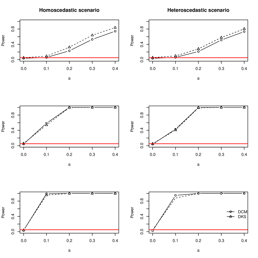
Figure 1: Power curves. Rejection probabilities of the proposed tests for nominal level 5% (red line), for $n=$ 1000, 3000 and 6000 (upper, middle and lower panels, respectively) and for both scenarios (left and right panels, respectively)

Finally, note that in order to obtain the results of the simulations, we have used wild bootstrap and we have selected the bandwidth (both in the original samples and in the bootstrap replicates) by means of cross-validation. However, although the whole results are not shown, we have also evaluated both the selected bootstrap procedure and the effect of the smoothing parameter. Regarding to the resampling technique, the simple bootstrap was also used; and two new situations were considered for the bandwidth: (i) to use cross-validation for obtaining the bandwidth for the original samples and then to fix these in the bootstrap replicates, (ii) to fix some bandwidths a priori. In all cases, poor results were obtained (lower powers and poorer approximations of type I error, especially with small sample sizes) when compared to those based on the the approximation exposed here.

The last conducted simulation aims to assess the performance of the Algorithm 1, i.e., the whole procedure. We compare our method with the procedure recently developed by Vogt and Linton (2017). The method aims to classify nonparametric functions in the longitudinal data framework. We have kept exactly the scenario described in Section 5 of the above mentioned paper. Then, for $j=1,\ldots,120$, the regression model given in (1) is considered with

$$m_{j}(X_{j})=\left\{{\begin{tabular}[]{lcc}$0$ \hskip 137.99603pt {\text{i}f}\quad$j\leq 50$,\\ $1-2X_{j}$ \hskip 108.12054pt {\text{i}f} \quad$51<j\leq 80$,\\ $0.75\hskip 2.84544pt{\rm tan^{-1}}\hskip 1.42271pt10(\hskip 2.84544ptX_{j}-0.6)$ \hskip 36.98866pt {\text{i}f} \quad$81<j\leq 100$,\\ $2.5\hskip 2.84544pt{\rm}(1-X_{j}^{2})^{4}\hskip 1.42271pt\mathds{1}(|{X_{j}}|\leq 1)$ \hskip 32.15175pt {\text{i}f} \quad$101<j\leq 110$,\\ $1.75\hskip 2.84544pt{\rm tan^{-1}}\hskip 1.42271pt5(X_{j}-0.6)+0.75$ \hskip 15.07993pt {\text{i}f} \quad$111<j\leq 120$,\\ \end{tabular}}\right.$$

being $X_{j}$ the explanatory covariate drawn from a uniform distribution on the interval $[0,1]$, and $\varepsilon_{j}$ the error distributed in accordance to a normal distribution $N(0,1.3)$. The simulation study was carried out under different sample sizes $n_{j}=100,150,200$ taking into account the test statistic $D_{CM}$. The remainder parameters of the simulation (number of simulation runs and number of bootstrap replicates) were kept as in the previous two scenarios.

In order to perform correctly, the Algorithm 1 must reject the first null hypothesis, $H_{0}(1)$, continues, rejects again the second one, $H_{0}(2)$, and so on until it accepts $H_{0}(5)$. Results of this simulation are shown in Table 4 which refers to the number of times that the procedure works well (in %) selecting the number of groups $K$ and using a nominal level of 5 %.

Table 4: Number of times in % (of 1000 repetitions) that the Algorithm 1 selects the number of groups using a nominal level of 5%.

		Number of groups
$n_{j}$	4	5	6	7	8	9	10
100	0.2	94.3	4.1	1.1	0.1	0.1	0.1
150	0.0	94.5	4.4	0.9	0.1	0.1	0.0
200	0.0	95.2	3.7	0.7	0.4	0.0	0.0

Results reported in Table 4 reveal a good behaviour of the proposed Algorithm 1, with rates of success around 95%, coming quite close to the $(1-\alpha)$ established. Already for the smallest samples size $n_{j}=100$, our procedure selects the true number of groups $K=5$ in 94.3% of the times unlike the results obtained by the method proposed in Vogt and Linton (2017) that show the 75% of the times. Moreover, there is a slight improvement on the proportion of success as the sample size increases.

To measure how well the procedure assigns each curve ($J=120$) to their correct group ($G_{1},\ldots,G_{5}$), the number of curves wrongly classified was analysed. Figure 2 shows the distribution of this variable for the different sample size ($n_{j}=100,150,200$). Particularly, it is shown the number of times in which a certain number of wrong assignments is obtained. Note that as the sample size increases, so does the number of correctly classified curves. For $n_{j}=100$ our procedure gives satisfactory results taking into account that at most five curves are wrongly classified in 90% of cases. At a sample size of $n_{j}=150$ our procedure is able to classify correctly all the curves in about 70% of the cases. Finally, for the biggest sample size, all the curves are correctly classified in 91% of the cases and most of the wrong classifications are due to the error in only one single curve out of a total of 120. It should be mentioned that these results are quite better regarding to those ones obtained by Vogt and Linton (2017) in which, considering the best scenario ($n_{j}=200$), all the curves are correctly classified about 80% of cases.

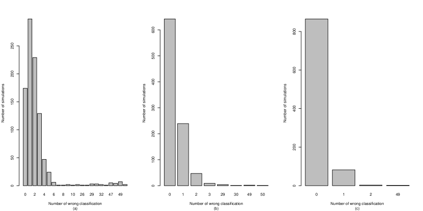
Figure 2: Simulation results for the estimation of the groups $G_{1},\dots,G_{5}$. (a)–(c) distributions of the number of wrong assignments for the Algorithm 1 (without Holm’s correction) and sample sizes $n_{j}=100,150,200$, respectively

4 Application to real data

Our methodology is applied to the study of the geometry of a tunnel through the analysis of a set of cross-sections. These sections were obtained by adjusting a point cloud collected with a RIEGL LMS.Z390 time of flight terrestrial laser scanner (TLS). It has a maximum range of about 400 m for objects with reflectance greater than $80\%$ and 6 mm nominal accuracy for a single point to a distance of 50 m. The capture rate is 8000 data points/second.

Terrestrial laser scanning is a ground based technique to measure the position and dimension of objects in a three dimensional space. Thereby, a laser beam is emitted from a laser light source and used to scan the surface of surrounding objects. The distance between the scanner and the object is determined by the time of flight principle. The laser range finder sends a laser pulse towards the object and measures the time taken by the pulse to be reflected from the target and returned to the sender. Also horizontal and vertical angles from the center of the scanner to the point are measured. Then the coordinates of the points are calculated using polar coordinates.

The tunnel was made by drilling and blasting. It is approximately circular and its theoretical diameter is 9 m. The cross-section of the tunnel should be constant throughout the tunnel but, in drill and blast, there can be over-break amounting to 10 to $20\%$ of the excavated cross-sectional area, which must be removed and possibly refilled. In the case of an insufficient excavation, the cross-section must be expanded by mechanical or manual methods. This represents a significant increase in the cost of the work.

Figure 3 shows the point cloud of the tunnel obtained with the TLS. Although the irregularities of its surface can be visually appreciated, it is of interest to know if the tunnel section is, in general terms, homogeneous or if, on the contrary, there are different areas of homogeneous section. The engineers could take advantage of this information to plan activities to rebuild the tunnel. Thus, it is very interesting to distinguish between areas of the tunnel that need to be refilled from those that are under-excavated and, consequently, need to be widened. It also can provide useful information regarding the mechanical characteristics of the materials. Moreover, our methodology allows taking into account the fact that some differences between the profiles could be due to the noise associated to the point cloud. Then small differences between the profiles that could have their origin in the measuring system are not computed as real differences in the tunnel.

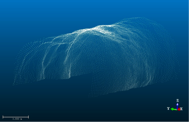
Figure 3: Tunnel point cloud. Tunnel measured with the terrestrial laser scanner

In order to determine the homogeneity of the tunnel, a data set of $n=$ 16 075 coordinates constituted by 66 cross-sections were obtained from the point cloud in Cartesian coordinates. The cross-sections were obtained by the intersection of the plane perpendicular to the axis of the tunnel and the 3D model created from the point cloud. For $j=1,\ldots,66$ sections, the point cloud measured with the TLS provides $(X_{j},Y_{j})$ coordinates. As the cross-sections given in Cartesian coordinates are not univariate functions, we first perform a transformation of the coordinates. The Cartesian coordinates $(X_{j},Y_{j})$ can be converted to polar coordinates $(r_{j},\alpha_{j})$ given by

$$(r_{j},\alpha_{j})=\left({\sqrt{X_{j}^{2}+Y_{j}^{2})},\arctan\left({{Y_{j}}/{X_{j}}}\right)}\right)$$

being $r$ the distance to each point and $\alpha$ the polar angle. Then, we use our proposed approach in the following regression models

$$r_{j}=m_{j}(\alpha_{j})+\varepsilon_{j}\quad\text{for}\quad j=1,\ldots,66.$$

The application of the proposed methodology —using the test statistics $D_{CM}$— indicates that, for a nominal level of 5%, the null hypothesis is rejected (with p-values lower than 0.01) until $K=5$ (with a p-value of 0.45) and therefore the cross-section $m_{1},\ldots,m_{66}$ can be grouped in five groups.

The estimated regression curves in polar coordinates given by $(\alpha_{j},\hat{m}_{j}(\alpha_{j}))$ for $j=1,\ldots,66$ are drawn in the left panel of Figure 4. Curves assigned to each group are plotted with the same color. The differences between groups are almost visually appreciable. Additionally, in order to graphically assess the analysis, the curves are shown in Cartesian coordinates using the transformation $\left({\hat{m}_{j}(\alpha_{j})\cos(\alpha_{j}),\hat{m}_{j}(\alpha_{j})\sin(\alpha_{j})}\right)$ (see right panel of Figure 4).

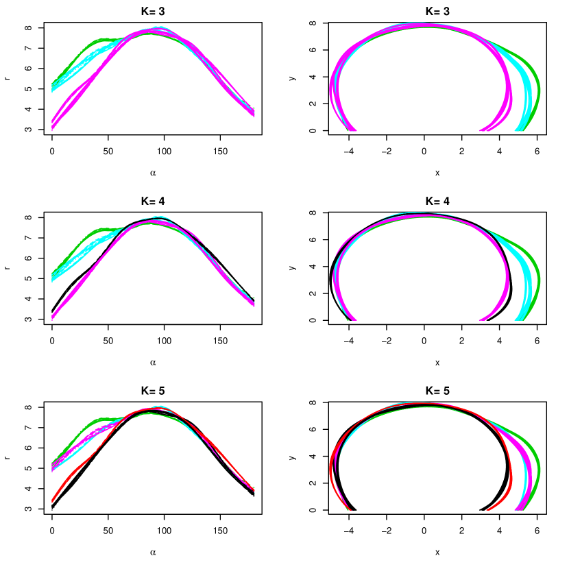
Figure 4: Estimated tunnel regression curves. The curves are colored according to the groups to which they belong. Upper, middle and lower panels correspond to these curves assigned into three ($K=3$), four ($K=4$) and five groups ($K=5$), respectively. Left and right panels are the estimates in polar and Cartesian coordinates, respectively.

Finally, Figure 5 depicts the spatial distribution of the cross-sections along the tunnel. A specific color is assigned for each section according to the group in which it belongs. As can be appreciated, there are two non-consecutive areas that belong to the same group (printed in black). It is also clear that three of the five groups (magenta, blue and green profiles) correspond to areas of the tunnel with a big over-excavation. The differences between them tell us that different coatings of shotcrete are needed for each of the three areas.

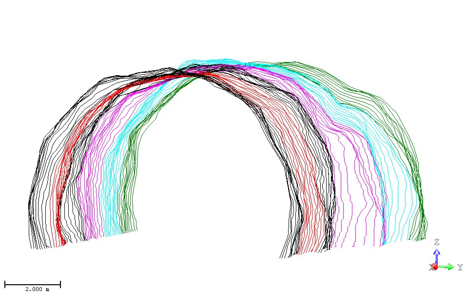
Figure 5: Spatial distribution of tunnel profiles. A specific color is assigned for each section according to the group to which it belongs (in this case five groups, $K=5$).

The good performance of the proposed procedure in terms of spatial distribution should be highlighted. The cross-sections which are spatially close belong to the same group, and accordingly, this provides an easy interpretation of results. Therefore, the identification of homogeneous areas allows a better planning of the work to build the final section of the tunnel, which should fit with the theoretical one.

5 Conclusion

Several nonparametric procedures have been proposed for the comparison of regression functions, however they are no fully informative when the null hypothesis is rejected. This is especially important in practice and in situations where the number of $J$ curves is large enough. In order to solve this situation, we proposed a new procedure that let us not only testing the equality of nonparametric regression curves but also grouping them if they are not equal. Insofar as our comprehensive simulation studies are concerned, we have shown that the results are satisfactory (both in terms of type I error and power) and indicate similar or even better performance than other procedures used in the literature.

The methodology has been applied to a tunnel inspection work addressed to determine heterogeneities in the tunnel geometry. By grouping a set of cross-sections of the tunnel surface it has been possible to identify five areas with significant differences in their geometry.

It is worth mentioning that software in the form of an R package named clustcurv Villanueva et al. (2020); Villanueva and Sestelo (2020) was developed implementing the proposed method which seems to be stable and computational efficient. clustcurv is available from the Comprehensive R Archive Network (CRAN) at https://cran.r-project.org/web/packages/clustcurv and can be called to group multiple nonparametric curves both in the regression and in the survival framework.

Although the proposed test is designed for detecting groups of regression curves with continuous response, it seems that the extension to other responses such as Bernoulli, Poisson or other parametric families can be achieved without much effort. Moreover, our methodology suffers from the limitation of solely being able to address a single continuous covariate, few further work is nevertheless needed to extend the proposed methodology to the case of multiple covariates.

Even though two different clustering techniques have been implemented in the algorithms proposed to determine groups of curves, the reach of this work might be expanded allowing more clustering techniques such as K-medoids (Kaufman and Rousseeuw, 1990) or Mean-Shift algorithms (Keinosuke and Hostetler, 1975). Finally, a more challenging target is to consider the application of these methods to the Big Data environment where the classical bootstrap techniques can be prohibitively demanding.

References

- Abraham et al. (2003) Abraham, C., Cornillon, P. A., Matzner-Løber, E., and Molinari, N. (2003). Unsupervised curve clustering using b-splines. Scandinavian Journal of Statistics, 30(3):581–595.
- de Boor (2001) de Boor, C. A. (2001). A Practical Guide to Splines. Springer Verlag, New York.
- Delgado (1993) Delgado, M. A. (1993). Testing the equality of nonparametric regression curves. Statistics and Probability Letters, 17:199–204.
- Dette and Neumeyer (2001) Dette, D. and Neumeyer, N. (2001). Nonparametric analysis of covariance. The Annals of Statistics, 29:1361–1400.
- Efron (1979) Efron, B. (1979). Bootstrap methods: another look at the jackknife. The Annals of Statistics, 7:1–26.
- Efron and Tibshirani (1993) Efron, E. and Tibshirani, R. J. (1993). An introduction to the Bootstrap. Chapman and Hall, London.
- Fan and Gijbels (1996) Fan, J. and Gijbels, I. (1996). Local polynomial modelling and its applications. Number 66 in Monographs on statistics and applied probability series. Chapman & Hall.
- Fan and Marron (1994) Fan, J. and Marron, J. (1994). Fast implementation of nonparametric curve estimators. Journal of Computational and Graphical Statistics, 3:35–56.
- García-Escudero and Gordaliza (2005) García-Escudero, L. A. and Gordaliza, A. (2005). A proposal for robust curve clustering. Journal of Classification, 22(2):185–201.
- Golub et al. (1979) Golub, G., Heath, M., and Wahba, G. (1979). Generalized cross-validation as a method for choosing a good ridge parameter. Technometrics, 21(2):215–223.
- González-Manteiga and Cao (1993) González-Manteiga, W. and Cao, R. (1993). Testing the hypothesis of a general linear model using nonparametric regression estimation. Test, 2(1):223–249.
- González-Manteiga and Crujeiras (2013) González-Manteiga, W. and Crujeiras, R. M. (2013). An updated review of Goodness-of-Fit tests for regression models. Test, 22:361–411.
- Hall and Hart (1990) Hall, P. and Hart, J. D. (1990). Bootstrap test for difference between means in nonparametric regression. Journal of the American Statistical Association, 85(412):1039–1049.
- Härdle and Mammen (1993a) Härdle, W. and Mammen, E. (1993a). Comparing nonparametric versus parametric regression fits. The Annals of Statistics, 21(4):1926–1947.
- Härdle and Mammen (1993b) Härdle, W. and Mammen, E. (1993b). Testing parametric versus nonparametric regression. Annals of Statistics, 21:1926–1947.
- Jain and Dubes (1988) Jain, A. K. and Dubes, R. C. (1988). Algorithms for clustering data. Prentice-Hall, Inc., Upper Saddle River, NJ, USA.
- Kauermann and Opsomer (2003) Kauermann, G. and Opsomer, J. (2003). Local Likelihood Estimation in Generalized Additive Models. Scandinavian Journal of Statistics, 30:317–337.
- Kaufman and Rousseeuw (1990) Kaufman, L. and Rousseeuw, P. J. (1990). Finding Groups in Data: An Introduction to Cluster Analysis. John Wiley.
- Keinosuke and Hostetler (1975) Keinosuke, F. and Hostetler, L. D. (1975). The estimation of the gradient of a density function, with applications in pattern recognition. IEEE Transactions on Information Theory, 21(1):32–40.
- King et al. (1991) King, E., Hart, J. D., and Wehrly, T. E. (1991). Testing the equality of two regression curves using linear smoothers. Statistics and Probability Letters, 12(3):239–247.
- Kulasekera (1995) Kulasekera, K. B. (1995). Comparison of regression curves using quasi-residuals. Journal of the American Statistical Association, 90(431):1085–1093.
- Lang and Brezger (2004) Lang, S. and Brezger, A. (2004). Bayesian p-splines. Journal of Computational and Graphical Statistics, 13:183–212.
- Liu (1988) Liu, R. Y. (1988). Bootstrap Procedures under some Non-I.I.D. Models. The Annals of Statistics, 16(4):1696–1708.
- Macqueen (1967) Macqueen, J. B. (1967). Some methods of classification and analysis of multivariate observations, volume 1. Proceedings of the Fifth Berkeley Symposium on Mathematical Statistics and Probability (Univ. of Calif. Press).
- Mammen (1993) Mammen, E. (1993). Bootstrap and Wild Bootstrap for High Dimensional Linear Models. The Annals of Statistics, 21(1):255–285.
- Pardo-Fernández et al. (2007) Pardo-Fernández, J. C., Van Keilegom, I., and González-Manteiga, W. (2007). Testing for the equality of k regression curves. Statistica Sinica, 17:1115–1137.
- Park et al. (2014) Park, C., Hannig, J., and Kang, K.-H. (2014). Nonparametric comparison of multiple regression curves in scale-space. Journal of Computational and Graphical Statistics, 23(3):657–677.
- Park and Kang (2008) Park, C. and Kang, K.-H. (2008). Sizer analysis for the comparison of regression curves. Computational Statistics and Data Analysis, 52(8):3954–3970.
- Rosenblatt (1975) Rosenblatt, M. (1975). A quadratic measure of deviation of two-dimensional density estimates and a test of independence. The Annals of Statistics, 3(1):1–14.
- Ruppert et al. (1995) Ruppert, D., Sheather, S. J., and Wand, M. P. (1995). An effective bandwidth selector for local least squares regression. Journal of the American Statistical Association, 90(432):1257–1270.
- Sestelo and Roca-Pardiñas (2019) Sestelo, M. and Roca-Pardiñas, J. (2019). Testing critical points of non-parametric regression curves: application to the management of stalked barnacles. Journal of the Royal Statistical Society C, 68(4):1051–1070.
- Sestelo et al. (2017) Sestelo, M., Villanueva, N. M., Meira-Machado, L., and Roca-Pardiñas, J. (2017). npregfast: An R Package for Nonparametric Estimation and Inference in Life Sciences. Journal of Statistical Software, 82(12):1–27.
- Sestelo et al. (2016) Sestelo, M., Villanueva, N. M., and Roca-Pardiñas, J. (2016). npregfast: Nonparametric Estimation of Regression Models with Factor-by-Curve Interactions. R package version 1.4.0.
- Srihera and Stute (2010) Srihera, R. and Stute, W. (2010). Nonparametric comparison of regression functions. Journal of Multivariate Analysis, 101:2039–2059.
- Tarpey (2007) Tarpey, T. (2007). Linear transformations and the k-means clustering algorithm. The American Statistician, 61(1):34–40.
- Villanueva et al. (2020) Villanueva, N. M., , Sestelo, M., Meira-Machado, L., and Roca-Pardiñas, J. (2020). clustcurv: An r package for determining groups in multiple curves. Manuscript submitted for publication.
- Villanueva and Sestelo (2020) Villanueva, N. M. and Sestelo, M. (2020). clustcurv: Determining Groups in Multiple Curves. R package version 2.0.1.
- Villanueva et al. (2019) Villanueva, N. M., Sestelo, M., and Meira-Machado, L. (2019). A Method for Determining Groups in Multiple Survival Curves. Statistics in Medicine, 38:366–377.
- Vogt and Linton (2017) Vogt, M. and Linton, O. (2017). Classification of non-parametric regression functions in longitudinal data models. Journal of the Royal Statistical Society Series B, 79(1):5–27.
- Vogt and Linton (2020) Vogt, M. and Linton, O. (2020). Multiscale clustering of nonparametric regression curves. Journal of Econometrics, 216(1):305–325.
- Wand and Jones (1995) Wand, M. P. and Jones, M. C. (1995). Kernel Smoothing. Chapman & Hall: London.
- Wu (1986) Wu, C. F. J. (1986). Jackknife, Bootstrap and other resampling methods in regression analysis. The Annals of Statistics, 14(4):1261–1295.
- Young and Bowman (1995) Young, S. G. and Bowman, A. W. (1995). Nonparametric analysis of covariance. Biometrics, 51:920–931.