On the Moyal Star Product of Resurgent Series

Abstract

We analyze the Moyal star product in deformation quantization from the resurgence theory perspective. By putting algebraic conditions on Borel transforms, one can define the space of “algebro-resurgent series” (a subspace of $1$-Gevrey formal series in $i\hbar/2$ with coefficients in $\mathbb{C}\{q,p\}$), which we show is stable under Moyal star product.

1 Introduction

1.1  The Moyal star product of two formal series $\tilde{f}$ and $\tilde{g}$ in $\mathbb{C}[[t,q_{1},\ldots,q_{N},p_{1},\ldots,p_{N}]]$ is defined by the formula

$$\tilde{f}\star_{M}\tilde{g}\coloneqq\tilde{f}\,\tilde{g}+\sum_{k\geq 1}\,\frac{t^{k}}{2^{k}k!}\,\sum_{n=0}^{k}(-1)^{k-n}\mbox{$\begin{pmatrix}k\\ n\end{pmatrix}$}\Big{(}\partial_{p}^{n}\,\partial_{q}^{k-n}\tilde{f}\Big{)}\Big{(}\partial_{p}^{k-n}\,\partial_{q}^{n}\tilde{g}\Big{)}$$ (1.1)

when $N=1$, and by an analogous formula when the number of degrees of freedom $N$ is larger than $1$. We get a non-commutative associative algebra $\big{(}\mathbb{C}[[t,q_{1},\ldots,q_{N},p_{1},\ldots,p_{N}]],\star_{M}\big{)}$, the unit of which is the constant series $1$; the corresponding commutator induces a deformation of the Poisson bracket $\{.\,,.\}$ associated with the standard symplectic structure ${\mathrm{d}}p_{1}\wedge{\mathrm{d}}q_{1}+\cdots{\mathrm{d}}p_{N}\wedge{\mathrm{d}}q_{N}$, inasmuch as

$$\tilde{f}\star_{M}\tilde{g}-\tilde{g}\star_{M}\tilde{f}=t\big{\{}\tilde{f},\tilde{g}\big{\}}+O(t^{2}).$$ (1.2)

The main result of this paper is

Theorem A.

If $\tilde{f}$ and $\tilde{g}$ are algebro-resurgent series, then so is their Moyal star product $\tilde{f}\star_{M}\tilde{g}$.

Here, “algebro-resurgence” is a property of a formal series $\tilde{f}(t,q_{1},\ldots,q_{N},p_{1},\ldots,p_{N})$ defined in terms of its formal Borel transform $\hat{f}(\xi,q_{1},\ldots,q_{N},p_{1},\ldots,p_{N})$ with respect to $t$, which is required to be convergent, i.e. $\hat{f}(\xi,q_{1},\ldots,q_{N},p_{1},\ldots,p_{N})\in\mathbb{C}\{\xi,q_{1},\ldots,q_{N},p_{1},\ldots,p_{N}\}$, and to admit analytic continuation along all the paths which start close enough to the origin of $\mathbb{C}^{1+2N}$ and avoid a certain proper algebraic subvariety (which depends on $\tilde{f}$). More details will be given in due time.

This variant of Écalle’s definition of resurgence [Eca84], [Eca85] was introduced by M. Garay, A. de Goursac and D. van Straten in [GGS14], where they state the

Theorem B.

If $\tilde{f}$ and $\tilde{g}$ are algebro-resurgent series, then so is their standard star product

$$\tilde{f}\star_{S}\tilde{g}\coloneqq\sum_{k_{1},\cdots,k_{N}\geq 0}\frac{t^{k_{1}+\cdots+k_{N}}}{k_{1}!\cdots k_{N}!}\Big{(}\partial_{p_{1}}^{k_{1}}\cdots\partial_{p_{N}}^{k_{N}}\tilde{f}\Big{)}\Big{(}\partial_{q_{1}}^{k_{1}}\cdots\partial_{q_{N}}^{k_{N}}\tilde{g}\Big{)}.$$ (1.3)

However, their proof of Theorem B is not valid, due to a flaw in one of the key formulas presented in [GGS14]. In this paper, we will give the correct formula and develop somewhat different arguments that lead to a proof of Theorem B and help to deduce Theorem A as well.

1.2  We first give some background and motivation.

Ever since quantum mechanics started in the 1920s, quantization and semiclassical limit have become a central theme among a variety of areas in mathematics such as functional analysis, geometry and topology, representation theory, pseudo-differential operators and microlocal analysis and symplectic geometry, to name a few.

Conventional quantum mechanics are formulated in terms of linear operators on Hilbert space that realize the fundamental Canonical Commutation Relations (CCR), or of Feynman’s path integrals as conceived by Dirac and developed by Feynman to make the quantum picture more compatible with the classical one. Built upon Wigner, Weyl and Groenewold’s insights and pioneered by Moyal, deformation quantization is a third formulation, in full phase space, which evolved gradually into an autonomous theory, with its own complete internal logic, that is conceptually very appealing.

The idea of deformation quantization is to achieve the Heisenberg CCR by deforming the commutative algebra of functions on the phase space (classical observables) to a non-commutative associative algebra.

In [Moy49], Moyal defined the so-called Moyal star product $\star_{M}$ in relation with statistical properties of quantum mechanics. For one degree of freedom, the standard Poisson structure for functions $f(q,p)$ and $g(q,p)$ in $\mathbb{R}^{2}$ being

$$\{f,g\}=\frac{\partial f}{\partial p}\frac{\partial g}{\partial q}-\frac{\partial f}{\partial q}\frac{\partial g}{\partial p}=\mu\circ P(f\otimes g),\quad\text{with}\enspace P\coloneqq\frac{\partial}{\partial p}\otimes\frac{\partial}{\partial q}-\frac{\partial}{\partial q}\otimes\frac{\partial}{\partial p},$$

where $\mu$ is the usual pointwise product of functions, the Moyal star product of two classical observables is the formal series in $t$ obtained as

$$f\star_{M}g=\mu\circ\exp\Big{(}\frac{tP}{2}\Big{)}(f\otimes g)=\mu\circ\Big{(}\mathop{\hbox{{\rm Id}}}\nolimits+\sum_{k\geq 1}\frac{t^{k}}{2^{k}k!}P^{k}\Big{)}(f\otimes g)$$ (1.4)

with

$$P^{k}=\sum_{n=0}^{k}(-1)^{k-n}\mbox{$\begin{pmatrix}k\\ n\end{pmatrix}$}(\partial_{p}\,{\otimes}\,\partial_{q})^{n}(\partial_{q}\,{\otimes}\,\partial_{p})^{k-n}=\sum_{n=0}^{k}(-1)^{k-n}\mbox{$\begin{pmatrix}k\\ n\end{pmatrix}$}\partial_{p}^{n}\,\partial_{q}^{k-n}\,{\otimes}\,\partial_{p}^{k-n}\,\partial_{q}^{n}.$$

Here, $t$ is the deformation parameter, taken to be ${i\hbar}$ in quantum mechanics. When extended to $C^{\infty}(\mathbb{R}^{2N})[[t]]$, the Moyal star product is a non-commutative associative product. We have $f\star_{M}g=fg+\frac{t}{2}\{f,g\}+O(t^{2})$, hence

$$[f,g]_{M}\coloneqq\frac{1}{t}(f\star_{M}g-g\star_{M}f)=\{f,g\}+O(t),$$ (1.5)

we thus recover the Poisson algebra structure of the classical observables in the limit $\hbar=t/i\to 0$. Moreover

$$p\star_{M}q-q\star_{M}p=t,\quad\text{{\emph{i.e.}}\ }\enspace[p,q]_{M}=1.$$

The extension to $N\geq 1$ degrees of fredom is obtained by replacing $P$ by

$$P=\sum_{j=1}^{N}\Big{(}\frac{\partial}{\partial p_{j}}\otimes\frac{\partial}{\partial q_{j}}-\frac{\partial}{\partial q_{j}}\otimes\frac{\partial}{\partial p_{j}}\Big{)}$$ (1.6)

in (1.4), so that (1.5) still holds. Moreover, the CCR are realized: $[p_{i},q_{i}]_{M}=1$ and $[p_{i},q_{j}]_{M}=[p_{i},p_{j}]_{M}=[q_{i},q_{j}]_{M}=0$ for $i\neq j$.

The Moyal star product can be viewed as a non-commutative associative deformation of the usual product of functions. The idea to view Quantum Mechanics as a deformation of Classical Mechanics was promoted by Bayen-Flato-Fronsdal-Lichnerowicz-Sternheimer [BFFL78] in the 1970s and led to what is now called Deformation Quantization Theory.

For general symplectic manifolds, the existence of a star product was proved in [DWL83] and [Fed85], [Fed94]. In particular, Fedosov recursively constructed a star product through a canonical flat connection on the Weyl bundle.

For an arbitrary Poisson structure $\pi$ on $\mathbb{R}^{N}$, Kontsevich ([Kon03]) constructed an intriguing explicit formula for its deformation quantization:

$$f\star_{K}g=fg+\sum_{k\geq 1}t^{k}\sum_{\Gamma\in G_{k}}c_{\Gamma}B_{\Gamma,\pi}(f,g),$$ (1.7)

where each $G_{k}$ is a suitable collection of graphs, the $c_{\Gamma}$’s are universal coefficients, and the $B_{{\Gamma},\pi}$’s are polydifferential operators depending on the graph ${\Gamma}$ and the Poisson structure $\pi$. Recently, a deep connection between these universal coefficients $c_{\Gamma}$ and multiple zeta values has been brought to light [BPP20].

For a general Poisson manifold $(M,\pi)$, the existence of a star product that satisfies the analogue of (1.5) is a consequence of the formality theorem which establishes an $L_{\infty}$ quasi-isomorphism between two differential graded Lie algebras (DGLAs): the Hochschild complex of the associative algebra $A=C^{\infty}(M)$ and its cohomology.

1.3  It is known after Dyson [Dys52] and others that, in quantum field theory, almost all the series in $\hbar$ describing physical quantities are divergent and must be interpreted as giving asymptotic information. In quantum mechanics, this can even be traced back to as early as Birkhoff. When Voros developed the exact WKB theory [Vor83] to study the spectrum of Sturm-Liouville operators, he already conjectured the resurgent character of these series. Resurgence Theory was then a new perspective, initiated by Écalle ([Eca81], [Eca85]), to deal with asymptotic series. Écalle immediately clarified and confirmed Voros’ conjecture in [Eca84] and [Eca85]. Pham and his collaborators devoted a lot of energy to make the whole picture complete in [Pha88] and a series of papers in the 1990s, culminating in the proof of the conjectural formula proposed by Zinn-Justin [ZJ83] on multi-instanton expansions in quantum mechanics (however they had to rely on a resurgence conjecture stated in [Eca84], the proof of which has not yet been given).

In a nutshell, Resurgence Theory deals with formal series $\widetilde{\varphi}(t)=\sum_{n\geq 0}a_{n}t^{n}$ (in applications to physics, the coefficients $a_{n}$ may be functions on the configuration space or the phase space) and their formal Borel transforms $\widehat{\varphi}(\xi)$, with

$$\text{formal Borel transform}\;\beta\colon\thinspace\widetilde{\varphi}(t)=\sum_{n\geq 0}a_{n}t^{n}\mapsto\widehat{\varphi}(\xi)=\sum_{n\geq 0}a_{n}\frac{\xi^{n}}{n!}$$ (1.8)

and imposes convergence of $\widehat{\varphi}(\xi)$ and suitable conditions on its analytic continuation, so as to be able to analyse the various “Borel-Laplace sums” $\mathscr{S}^{\theta}\widetilde{\varphi}(t)=\int_{0}^{\mathrm{e}^{{\mathrm{i}}{\theta}}\infty}\mathrm{e}^{-\xi/t}\widehat{\varphi}(\xi){\mathrm{d}}t/t$, for all non-singular directions ${\theta}$, which are all asymptotic to $\widetilde{\varphi}(t)$ as $\lvert t\rvert\to 0$ but differ by exponentially small quantities. One requires the analytic continuation of the convergent germ $\widehat{\varphi}(\xi)$, roughly speaking, to have at worse isolated singularities—more precisely, to be “$\Omega$-continuable” with a certain prescribed set $\Omega$ of potential singular points [Eca81], [Sau13]; or “endlessly continuable” [CNP93]; or “continuable without a cut” [Eca85] (in order of increasing generality).

Another variant of this property of continuability in the Borel plane was introduced in [GGS14] under the name “algebro-resurgence”, that was designed for situations where the coefficients $a_{n}$ depend analytically on affine variables $(q,p)\in\mathbb{C}^{2N}$: the singular locus of $\widehat{\varphi}(\xi,q,p)$ is required to be a proper algebraic subvariety of $\mathbb{C}^{1+2N}$, the germ $\widehat{\varphi}(\xi,q,p)$ should have analytic continuation along all the paths that avoid it; in particular, for fixed $(q,p)$, only finitely many singular points can exist in the Borel plane. It is with this version of resurgence that we will work throughout this article.

1.4  Our initial motivation was to understand Deformation Quantization and the explicit construction (1.7) of Kontsevich from the viewpoint of Resurgence Theory. But already at the level of the Moyal star product (1.4), even with analytic classical observables that do not depend on $t$, one can see that divergence of the series generically occurs, but with at most factorial growth due to the Cauchy inequalities. It is thus natural to consider the Moyal star product of two elements of $\widetilde{f}$ and $\widetilde{g}$ of $\mathbb{C}\{q_{1},\ldots,q_{N},p_{1},\ldots,p_{N}\}[[t]]$ and to enquire on $\beta(\widetilde{f}\star_{M}\widetilde{g})$ in terms of $\beta\widetilde{f}$ and $\beta\widetilde{g}$, i.e. to investigate the Borel counterpart of the Moyal star product:

$$\widehat{f}*_{M}\widehat{g}\coloneqq\beta\big{(}\beta^{-1}\widehat{f}\star_{M}\beta^{-1}\widehat{g}\big{)}.$$ (1.9)

This is what Garay, de Goursac and van Straten did in [GGS14] with the “standard star product” $\star_{S}$ defined by (1.3), which is a star product equivalent to the Moyal one (see Section 2). They considered

$$\widehat{f}*_{S}\widehat{g}\coloneqq\beta\big{(}\beta^{-1}\widehat{f}\star_{S}\beta^{-1}\widehat{g}\big{)}$$ (1.10)

with a view to proving Theorem B: supposing that $\widetilde{f}$ and $\widetilde{g}$ are algebro-resurgent series, i.e. that $\widehat{f}$ and $\widehat{g}$ are algebro-resurgent germs, is it true that $\widehat{f}*_{S}\widehat{g}$ is an algebro-resurgent germ (and hence that $\widetilde{f}\star_{S}\widetilde{g}$ is an algebro-resurgent series)?

However, the analysis in [GGS14] relies on an integral representation of $*_{S}$ that is flawed, thus invalidating the key Proposition 3.3 and the purported proof of Theorem B in that article. In Section 2, we will give another integral representation of $*_{S}$, formula (2.20). The correct formula is more intricate than that of [GGS14]; therefore, following the analytic continuation of $\widehat{f}*_{S}\widehat{g}$ (where both factors are supposed to be algebro-resurgent) requires considerably more work.

For the sake of clarity, we will begin in Section 2 with the case of one degree of freedom and give in Lemma 2.3 the formula for $*_{S}$ for that case. It is a mixture of convolution and Hadamard product (which has the classical integral representation (6.1)); more specifically, the formula involves the Hadamard product with respect to ${\zeta}$ of the Taylor expansions $\widehat{f}(\xi_{1},q,p+{\zeta})\odot\widehat{g}(\xi_{2},q+{\zeta},p)$ and then a convolution-like integration with respect to $\xi_{1}$ and $\xi_{2}$.

Analytic continuation of convolution is a classical topic in Resurgence Theory [Eca81], [CNP93], [Sau13], [MS16]. We will adapt these techniques to our more intricate situation in Section 5. The analytic continuation of the Hadamard product of two $\Omega$-continuable germs has been treated in [LSS20], with a possibly infinite singular locus $\Omega$; our situation is simpler inasmuch as it involves only finite singular loci in the Borel plane, as we will see in Section 6 devoted to the Hadamard part of the formula for $*_{S}$.

The technique for following the analytic continuation of $\widehat{f}*_{S}\widehat{g}$ in the case of $N$ degrees of freedom is sketched in Section 7. This will lead us to a proof of Theorem B that follows a path rather different than that of [GGS14]. Using the concrete form of the equivalence between the Moyal and standard star products $\star_{M}$ and $\star_{S}$, we will be able to relate $*_{M}$ and $*_{S}$ by an integral transform, and deduce that

$\widehat{f}$ and $\widehat{g}$ algebro-resurgent germs $\quad\Longrightarrow\quad$ $\widehat{f}*_{M}\widehat{g}$ algebro-resurgent germ,

which is equivalent to Theorem A.

Hence, algebro-resurgent series form a subalgebra of $\big{(}\mathbb{C}\{q_{1},\ldots,q_{N},p_{1},\ldots,p_{N}\}[[t]],\star_{S}\big{)}$ or of $\big{(}\mathbb{C}\{q_{1},\ldots,q_{N},p_{1},\ldots,p_{N}\}[[t]],\star_{M}\big{)}$.

1.5  The paper is organized as follows.

1. Section 2 deals with definitions, examples and elementary properties for the Moyal and standard star products, $\star_{M}$ and $\star_{S}$, and their Borel counterparts $*_{M}$ and $*_{S}$. It also contains the integral representation formulas that will be used in the rest of the article.

2. Section 3 deals with the definition of algebro-resurgent series and algebro-resurgent germs, and states three lemmas that are instrumental in our proof of Theorems A and B.

3. Section 4 introduces the notion of a multivariate polynomial that is “simple with respect to one of its variables”, as an algebraic preparation to handle more conveniently the smooth algebraic varieties which appear in the singular loci in the Borel plane.

4. Section 5 deals with the “convolution part” of our formula for $*_{S}$.

5. Section 6 deals with the “Hadamard part” of the formula.

6. Section 7 explains how to adapt the proof from $N=1$ to $N$ arbitrary.

2 Borel counterparts of the Moyal and standard star products

2.1  The star product $\star_{M}$ is defined by formula (1.1) if $N=1$, or (1.4) with $P$ as in (1.6) for general $N\geq 1$. These formulas make sense in $\mathbb{C}\{q_{1},\ldots,q_{N},p_{1},\ldots,p_{N}\}[[t]]$ as well as in

$$\widetilde{\mathcal{Q}}_{2N+1}\coloneqq\mathbb{C}[[q_{1},\ldots,q_{N},p_{1},\ldots,p_{N}]][[t]]=\mathbb{C}[[t,q_{1},\ldots,q_{N},p_{1},\ldots,p_{N}]].$$

The same is true for $\star_{S}$, which is defined by the formula (1.3) or, equivalently

$$f\star_{S}g=\mu\circ\exp\bigg{(}t\sum_{j=1}^{N}\Big{(}\frac{\partial}{\partial p_{j}}\otimes\frac{\partial}{\partial q_{j}}\Big{)}\bigg{)}(f\otimes g).$$ (2.1)

Recall that the formal deformation parameter is $t={i\hbar}$.

It is well-known that $\star_{S}$ and $\star_{M}$ are equivalent, in the sense that there is a “transition operator” $T$ mapping the former to the latter: $T(f\star_{S}g)=(Tf)\star_{M}(Tg)$. It is sufficient to take

$$T\coloneqq\exp\Big{(}-\frac{i\hbar}{2}\sum_{1\leq j\leq N}\partial_{q_{j}}\partial_{p_{j}}\Big{)}=\exp\Big{(}-\frac{t}{2}\sum_{1\leq j\leq N}\partial_{q_{j}}\partial_{p_{j}}\Big{)},$$ (2.2)

the inverse of which is given by $T^{-1}=\exp\big{(}\frac{t}{2}\sum\partial_{q_{j}}\partial_{p_{j}}\big{)}$. In other words, we have

$$T\colon\thinspace\big{(}\widetilde{\mathcal{Q}}_{2N+1},\star_{S}\big{)}\to\big{(}\widetilde{\mathcal{Q}}_{2N+1},\star_{M}\big{)}\enspace\;\text{isomorphism of associative algebras.}$$

It is with $\star_{S}$ that we will work most of the time, because the formulas are simpler with it than with $\star_{M}$, hence we use the abbreviation

Notation 2.1.

From now on, we set $\star=\star_{S}$ for the standard star product, and $*=*_{S}$ for its Borel counterpart (1.10). We will call $*$ the “Borel-star product”.

Example 2.2.

Here is a simple example:

$$(tp)\star(tq)=t^{2}pq+t^{3},\enspace(tq)\star(tp)=t^{2}pq,\enspace(tp)\star_{M}(tq)=t^{2}pq+t^{3},\enspace(tq)\star_{M}(tp)=t^{2}pq-t^{3}.$$ (2.3)

Note that $T(t^{2}pq)=t^{2}pq-\frac{t^{3}}{2}$.

2.2  We are mostly interested in the subspace $\mathbb{C}\{q_{1},\ldots,q_{N},p_{1},\ldots,p_{N}\}[[t]]$ of $\widetilde{\mathcal{Q}}_{2N+1}$. However, it is important to realize that we cannot restrict ourselves to the too narrow subspace $\mathbb{C}\{t,q_{1},\ldots,q_{N},p_{1},\ldots,p_{N}\}$ consisting of formal series which converge in a neighbourhood of the origin in $\mathbb{C}^{2N+1}$, because even if $f$ and $g$ do not depend on $t$, their star product may be divergent. Here is a simple example taken from [GGS14], and a variant:

Examples.

The geometric series $(1-p)^{-1}$ and $(1-q)^{-1}$ give rise to a divergent series

$$(1-p)^{-1}\star(1-q)^{-1}=\sum_{k\geq 0}k!t^{k}\big{(}(1-p)(1-q)\big{)}^{-k-1}.$$ (2.4)

The logarithm series $\log(1-p)$ and $\log(1-q)$ give rise to a divergent series

$$\log(1-p)\star\log(1-q)=\log(1-p)\log(1-q)+\sum_{k\geq 1}\frac{(k-1)!}{k}t^{k}\big{(}(1-p)(1-q)\big{)}^{-k}.$$ (2.5)

Note however the $1$-Gevrey character with respect to $t$ of these examples: the coefficient of $t^{k}$ essentially has at most factorial growth, hence convergence is restored when $t^{k}$ is replaced by $\xi^{k}/k!$, i.e. their image by the formal Borel transform (1.8) belongs to the space of convergent series $\mathbb{C}\{\xi,q,p\}$. This is a general phenomenon: extending the definition of the formal Borel transform by the formula

$$\beta\colon\thinspace\widetilde{\varphi}=\sum_{n\geq 0}a_{n}(z_{1},\ldots,z_{r})t^{n}\in\mathbb{C}[[t,z_{1},\ldots,z_{r}]]\mapsto\widehat{\varphi}=\sum_{n\geq 0}a_{n}(z_{1},\ldots,z_{r})\frac{\xi^{n}}{n!}\in\mathbb{C}[[\xi,z_{1},\ldots,z_{r}]],$$ (2.6)

we call $1$-Gevrey formal series with respect to $t$ the elements of

$$\widetilde{\mathcal{Q}}_{r+1}\coloneqq\beta^{-1}\big{(}\widehat{\mathcal{Q}}_{r+1}\big{)}\subset\mathbb{C}[[t,z_{1},\ldots,z_{r}]],\quad\text{with}\enspace\widehat{\mathcal{Q}}_{r+1}\coloneqq\mathbb{C}\{\xi,z_{1},\ldots,z_{r}\}.$$ (2.7)

and we have, as noted in [GGS14],

Theorem C.

The subspace $\widetilde{\mathcal{Q}}_{2N+1}$ is stable under the Moyal star product $\star_{M}$, as well as under the standard product $\star=\star_{S}$.

The proof is a consequence of (2.21) in Lemma 2.7.

In the case of Examples (2.4) and (2.5), we find

$$\beta\big{(}(1-p)^{-1}\star(1-q)^{-1}\big{)}=\Big{(}1-\xi\big{(}(1-p)(1-q)\big{)}^{-1}\Big{)}^{-1}$$ (2.8)

$$\beta\big{(}\log(1-p)\star\log(1-q)\big{)}=\log(1-p)\log(1-q)+\operatorname{Li}_{2}\Big{(}\xi\big{(}(1-p)(1-q)\big{)}^{-1}\Big{)},$$ (2.9)

where

$$\operatorname{Li}_{2}(z)=\sum_{k\geq 1}\frac{z^{k}}{k^{2}}=-\int_{0}^{z}\frac{\log(1-{\zeta})}{{\zeta}}\,{\mathrm{d}}{\zeta}.$$ (2.10)

In fact, the divergent series (2.4) is essentially the famous Euler series, the most elementary example of resurgent series.

2.3  Recall that we have defined the Borel counterpart $*_{M}$ of the Moyal star product $\star_{M}$ by (1.9), and the Borel-star product $*=\star_{S}$, counterpart of the standard star product $\star$, by (1.10).

For the sake of simplicity, we begin with the case of one degree of freedom.

Lemma 2.3.

There is an integral representation of the Borel-star product in $\mathbb{C}[[\xi,q,p]]$ as follows:

$$\hat{f}\ast\hat{g}(\xi,q,p)=\frac{d^{3}}{d\xi^{3}}\int_{0}^{\xi}d\xi_{1}\int_{0}^{\xi-\xi_{1}}d\xi_{2}\int_{0}^{\xi-\xi_{1}-\xi_{2}}d\xi_{3}\int_{0}^{2\pi}\frac{d\theta}{2\pi}\hat{f}(\xi_{1},q,p+\sqrt{\xi_{3}}e^{-i\theta})\hat{g}(\xi_{2},q+\sqrt{\xi_{3}}e^{i\theta},p),$$ (2.11)

where the integrand is considered as element of $\mathbb{C}[e^{\pm i\theta}][[q,p,\xi_{1},\xi_{2},\sqrt{\xi_{3}}]]$ and integration in $\theta$ is performed termwise.

Moreover, if both factors are convergent, i.e. $\hat{f},\hat{g}\in\widehat{\mathcal{Q}}_{3}$, then so is their Borel-star product: $\hat{f}*\hat{g}\in\widehat{\mathcal{Q}}_{3}$.

Proof.

We expand $\hat{f}$ and $\hat{g}$:

$$\begin{split}\hat{f}\ast\hat{g}(\xi,q,p)=&\sum\limits_{m,n,s\geq 0}\frac{n!m!}{(n+m+s)!s!}(\partial_{p}^{s}f_{m})(\partial_{q}^{s}g_{n})\xi^{m+n+s}\\ =&\frac{d^{3}}{d\xi^{3}}\int_{0}^{\xi}d\xi_{1}\int_{0}^{\xi-\xi_{1}}d\xi_{2}\int_{0}^{\xi-\xi_{1}-\xi_{2}}d\xi_{3}\sum\limits_{n,m,s\geq 0}\frac{\partial_{p}^{s}f_{m}\partial_{q}^{s}g_{n}}{s!s!}\xi_{1}^{m}\xi_{2}^{n}\xi_{3}^{s}.\end{split}$$

Using the fact that the Hadamard product of two formal series $\phi(\xi)=\sum\limits_{s\geq 0}a_{s}\xi^{s}$ and $\psi(\xi)=\sum\limits_{t\geq 0}b_{t}\xi^{t}$ can be written as $\phi\odot\psi(\xi)=\frac{1}{2\pi}\int_{0}^{2\pi}\phi(\sqrt{\xi}e^{-i\theta})\psi(\sqrt{\xi}e^{i\theta})d\theta$ with termwise integration in $\mathbb{C}[e^{\pm i\theta}][[\sqrt{\xi}]]$, we get

$$\begin{split}\hat{f}\ast\hat{g}(\xi,q,p)=&\frac{d^{3}}{d\xi^{3}}\int_{0}^{\xi}d\xi_{1}\int_{0}^{\xi-\xi_{1}}d\xi_{2}\int_{0}^{\xi-\xi_{1}-\xi_{2}}d\xi_{3}\\ &\frac{1}{2\pi}\int_{0}^{2\pi}d\theta\sum\limits_{m,n\geq 0}f_{m}(q,p+\sqrt{\xi_{3}}e^{-i\theta})g_{n}(q+\sqrt{\xi_{3}}e^{i\theta},p)\xi_{1}^{m}\xi_{2}^{n}\\ =&\frac{d^{3}}{d\xi^{3}}\int_{0}^{\xi}d\xi_{1}\int_{0}^{\xi-\xi_{1}}d\xi_{2}\int_{0}^{\xi-\xi_{1}-\xi_{2}}d\xi_{3}\\ &\frac{1}{2\pi}\int_{0}^{2\pi}d\theta\hat{f}(\xi_{1},q,p+\sqrt{\xi_{3}}e^{-i\theta})\hat{g}(\xi_{2},q+\sqrt{\xi_{3}}e^{i\theta},p).\end{split}$$

Now, suppose $\hat{f},\hat{g}\in\widehat{\mathcal{Q}}_{3}=\mathbb{C}\{\xi,q,p\}$. The right hand side of (2.11) involves a function $G(\xi_{1},\xi_{2},s,q,p):=\int_{0}^{2\pi}\hat{f}(\xi_{1},q,p+se^{-i\theta})\hat{g}(\xi_{2},q+se^{i\theta},p)\frac{d\theta}{2\pi}$ which clearly belongs to $\mathbb{C}\{\xi_{1},\xi_{2},s,q,p\}$ (indeed, we can take $(s,\xi_{1},\xi_{2},q,p)$ close enough to origin). In fact, $G(\xi_{1},\xi_{2},s,q,p)=G(\xi_{1},\xi_{2},-s,q,p)$, hence $F(\xi_{1},\xi_{2},\xi_{3},q,p):=G(\xi_{1},\xi_{2},\sqrt{\xi_{3}},q,p)\in\mathbb{C}\{\xi_{1},\xi_{2},\xi_{3},q,p\}$ and the right hand side of (2.11) can be written as

$$\frac{d^{3}}{d\xi^{3}}\int_{0}^{\xi}d\xi_{1}\int_{0}^{\xi-\xi_{1}}d\xi_{2}\int_{0}^{\xi-\xi_{1}-\xi_{2}}d\xi_{3}F(\xi_{1},\xi_{2},\xi_{3},q,p),$$ (2.12)

hence it defines a holomorphic germ in $\mathbb{C}\{\xi,q,p\}$. ∎

The integral formula (2.11) differs from the one given in Proposition 3.3 of [GGS14], which is not correct. Take for instance $\hat{f}=\xi p$ and $\hat{g}=\xi q$: we know by the first equation in (2.3) that we must find

$$(\xi p)*(\xi q)=pq\frac{\xi^{2}}{2!}+\frac{\xi^{3}}{3!},$$ (2.13)

and the reader may check that our formula produces the right outcome, but not the formula from [GGS14], which yields a term $\frac{\xi^{3}}{2!}$ instead of $\frac{\xi^{3}}{3!}$.

Remark 2.4.

Instead of writing the Hadamard product $\phi\odot\psi(\xi)$ as we did in our proof, we could have used the integration variable ${\zeta}=\sqrt{\xi}\mathrm{e}^{{\mathrm{i}}{\theta}}$ and then the Cauchy theorem, which yields

$$\phi\odot\psi(\xi)=\frac{1}{2\pi i}\oint_{C}\phi(\frac{\xi}{z})\psi(z)\frac{dz}{z}\quad\text{with any circle}\enspace C\colon\thinspace{\theta}\mapsto c\,\mathrm{e}^{{\mathrm{i}}{\theta}}\enspace\text{of radius}\enspace c\in\big{(}\tfrac{|\xi|}{R_{\psi}},R_{\phi}\big{)},$$ (2.14)

where $R_{\phi}$ and $R_{\psi}$ are the radii of convergence of $\phi$ and $\psi$. Correspondingly, Formula (2.11) can be rewritten

$$\hat{f}\ast\hat{g}(\xi,q,p)=\frac{d^{3}}{d\xi^{3}}\int_{0}^{\xi}d\xi_{1}\int_{0}^{\xi-\xi_{1}}d\xi_{2}\int_{0}^{\xi-\xi_{1}-\xi_{2}}d\xi_{3}\oint_{C}\frac{dz}{2\pi iz}\hat{f}(\xi_{1},q,p+\frac{\xi_{3}}{z})\hat{g}(\xi_{2},q+z,p),$$ (2.15)

where $C$ is an appropriate circle.

Lemma 2.5.

If $\hat{f},\hat{g}\in\mathbb{C}[[\xi,q,p]]$, then

$$\begin{split}\hat{f}*_{M}\hat{g}&=\frac{d^{4}}{d\xi^{4}}\int^{\xi}_{0}d\xi_{1}\int^{\xi-\xi_{1}}_{0}d\xi_{2}\int^{\xi-\xi_{1}-\xi_{2}}_{0}d\xi_{3}\int^{\xi-\xi_{1}-\xi_{2}-\xi_{3}}_{0}d\xi_{4}\\ &(\frac{1}{2\pi i})^{2}\oint_{C_{1}}dz_{1}\oint_{C_{2}}dz_{2}\hat{f}(\xi_{1},q+z_{1},p+z_{2})\hat{g}(\xi_{2},q+\frac{\xi_{4}}{2z_{2}},p-\frac{\xi_{3}}{2z_{1}})\end{split}$$ (2.16)

with integration on appropriate circles $C_{1}$ and $C_{2}$.

Moreover, if both factors are convergent, i.e. $\hat{f},\hat{g}\in\widehat{\mathcal{Q}}_{3}$, then so is $\hat{f}*_{M}\hat{g}$.

Proof.

$$\begin{split}\text{RHS}=&\frac{d^{4}}{d\xi^{4}}\int^{\xi}_{0}d\xi_{1}\int^{\xi-\xi_{1}}_{0}d\xi_{2}\int^{\xi-\xi_{1}-\xi_{2}}_{0}d\xi_{3}\int^{\xi-\xi_{1}-\xi_{2}-\xi_{3}}_{0}d\xi_{4}\\ &\sum\limits_{n,m}\Big{(}\partial_{p}^{n}\partial_{q}^{m}\hat{f}(\xi_{1},q,p)\Big{)}\Big{(}\partial_{p}^{m}\partial_{q}^{n}\hat{g}(\xi_{2},q,p)\Big{)}\frac{(-1)^{m}}{2^{m+n}m!^{2}n!^{2}}\xi_{3}^{m}\xi_{4}^{n}\\ =&\frac{d^{2}}{d\xi^{2}}\int^{\xi}_{0}d\xi_{1}\int^{\xi-\xi_{1}}_{0}d\xi_{2}\\ &\sum\limits_{n,m,\alpha,\beta}\Big{(}\partial_{p}^{n}\partial_{q}^{m}f_{\alpha}(q,p)\xi_{1}^{\alpha}\Big{)}\Big{(}\partial_{p}^{m}\partial_{q}^{n}g_{\beta}(q,p)\xi_{2}^{\beta}\Big{)}\frac{(-1)^{m}}{2^{m+n}m!n!(n+m)!}(\xi-\xi_{1}-\xi_{2})^{n+m}\\ =&\text{LHS}.\end{split}$$

∎

The last statement in Lemma 2.5 can also be derived from the following integral representations of the Borel counterparts of $T$ and $T^{-1}$,

$$\widehat{T}\hat{f}\coloneqq\beta T\beta^{-1}\hat{f},\qquad\widehat{T}^{-1}\hat{f}=\beta T^{-1}\beta^{-1}\hat{f}.$$ (2.17)

Lemma 2.6.

For any $\hat{f}\in\mathbb{C}[[\xi,q,p]]$,

$$\widehat{T}\hat{f}=\frac{d}{d\xi}\int_{0}^{\xi}d\xi_{1}\frac{1}{2\pi i}\oint_{C}\hat{f}(\xi-\xi_{1},q+z,p-\frac{\xi_{1}}{2z})\frac{dz}{z},$$ (2.18)

$$\widehat{T}^{-1}\hat{f}=\frac{d}{d\xi}\int_{0}^{\xi}d\xi_{1}\frac{1}{2\pi i}\oint_{C}\hat{f}(\xi-\xi_{1},q+z,p+\frac{\xi_{1}}{2z})\frac{dz}{z},$$ (2.19)

with integration on appropriate circle $C$.

Moreover, if $\hat{f}$ is convergent, i.e. $\hat{f}\in\widehat{\mathcal{Q}}_{3}$, then so is $\widehat{T}\hat{f}$.

Proof.

$$\begin{split}\text{RHS}&=\frac{d}{d\xi}\int_{0}^{\xi}d\xi_{1}\frac{1}{2\pi i}\oint_{C}\sum\limits_{n,m}\frac{\partial^{n}_{q}\partial^{m}_{p}\hat{f}(\xi-\xi_{1},q,p)}{n!m!}{(-\frac{\xi_{1}}{2})^{m}}z^{n-m-1}dz\\ &=\frac{d}{d\xi}\int_{0}^{\xi}d\xi_{1}\sum\limits_{n}\frac{\partial^{n}_{q}\partial^{n}_{p}\hat{f}(\xi-\xi_{1},q,p)}{n!n!}(-\frac{\xi_{1}}{2})^{n}\\ &=\beta\big{(}\sum\limits_{n}\frac{\partial^{n}_{q}\partial^{n}_{p}\tilde{f}(t,q,p)}{n!}\cdot(-\frac{t}{2})^{n}\big{)}\\ &=\text{LHS}.\end{split}$$

∎

2.4  We now consider the case of an abitrary number of degrees of freedom, say $r$. We set $q=(q_{1},\cdots,q_{r})$ and $p=(p_{1},\cdots,p_{r})$. If $\hat{f}(\xi,q,p)=\sum\limits_{m=0}^{\infty}f_{m}(q,p)\xi^{m}$, $\hat{g}(\xi,q,p)=\sum\limits_{n=0}^{\infty}g_{n}(q,p)\xi^{n}$, then

$$\hat{f}\ast\hat{g}(\xi,q,p)=\sum_{m,n,k_{1},\cdots,k_{r}\geq 0}\frac{n!m!}{k_{1}!\cdots k_{r}!}(\partial_{p_{1}}^{k_{1}}\cdots\partial_{p_{r}}^{k_{r}}f_{m})(\partial_{q_{1}}^{k_{1}}\cdots\partial_{q_{r}}^{k_{r}}g_{n})\frac{\xi^{k_{1}+\cdots+k_{r}+n+m}}{(k_{1}+\cdots+k_{r}+n+m)!}.$$

Lemma 2.7.

There are integral representation formulas analogous to those of Lemmas 2.3, 2.5 and 2.6 for the case of $r$ degrees of freedom. For instance, for $\hat{f},\hat{g}\in\mathbb{C}[[\xi_{1},q_{1},\ldots,q_{r},p_{1},\ldots,p_{r}]]$, the formula generalising (2.11) is

$$\begin{split}\hat{f}\ast\hat{g}(\xi,q,p)=&\frac{d^{r+2}}{d\xi^{r+2}}\int^{\xi}_{0}d\xi_{1}\int^{\xi-\xi_{1}}_{0}d\xi_{2}\cdots\int_{0}^{\xi-\xi_{1}-\cdots-\xi_{r+1}}d\xi_{r+2}\big{(}\frac{1}{2\pi}\big{)}^{r}\overbrace{\int_{0}^{2\pi}\cdots\int_{0}^{2\pi}}^{r}d\theta_{1}\cdots d\theta_{r}\\ &\hat{f}(\xi_{r+1},q_{1},\cdots,q_{r},p_{1}+\sqrt{\xi_{1}}e^{-i\theta_{1}},\cdots,p_{r}+\sqrt{\xi_{r}}e^{-i\theta_{r}})\\ &\hat{g}(\xi_{r+2},q_{1}+\sqrt{\xi_{1}}e^{i\theta_{1}},\cdots,q_{r}+\sqrt{\xi_{r}}e^{i\theta_{r}},p_{1},\cdots,p_{r}).\end{split}$$ (2.20)

These formulas entail that

$$\hat{f},\hat{g}\in\widehat{\mathcal{Q}}_{2r+1}\quad\Longrightarrow\quad\hat{f}*\hat{g},\;\;\hat{f}*_{M}\hat{g},\;\;\widehat{T}\hat{f},\;\;\widehat{T}^{-1}\hat{f}\in\widehat{\mathcal{Q}}_{2r+1}.$$ (2.21)

3 Algebro-resurgent germs

Notation 3.1.

We shall use the following notation:

$$\mathbb{D}_{\tau}:=\{z\in\mathbb{C}\mid|z|<\tau\}.$$ (3.1)

We know that if $f\in\mathbb{C}\{z_{1},\cdots,z_{n}\}$, then there exists $\tau>0$, such that $f$ is the germ of a function holomorphic in the polydisc $\mathbb{D}_{\tau}^{n}\subset\mathbb{C}^{n}$. Following [GGS14], we set the

Definition 3.2.

The set of algebro-resurgent germs is defined as follows: for any non-negative integer $n$,

$$\begin{split}{\widehat{\mathcal{Q}}}^{\mathcal{A}}_{n+1}:=\Big{\{}&f\in\mathbb{C}\{\xi,z_{1},\cdots,z_{n}\}\mid\exists\text{ proper algebraic subvariety }V\subset\mathbb{C}^{n+1},\\ &s.t.\ f\ \text{admits analytic}\text{ continuation along any $C^{1}$ path $\gamma$ }\\ &\text{contained in $\mathbb{C}^{n+1}-V$ and having initial point $\gamma(0)$ close enough to~{}$0$}\Big{\}}.\end{split}$$ (3.2)

Here “$\gamma(0)$ close enough to $0$” means that $\gamma(0)\in\mathbb{D}_{\tau}^{n+1}$ where $\mathbb{D}_{\tau}^{n+1}$ is a polydisc where $f$ induces a holomorphic function.  

We denote by $\widehat{\mathcal{Q}}^{\mathcal{A}}$ the disjoint union of $\widehat{\mathcal{Q}}^{\mathcal{A}}_{i}$ :

$$\widehat{\mathcal{Q}}^{\mathcal{A}}:=\bigsqcup\limits_{i\in\mathbb{N}^{\ast}}\widehat{\mathcal{Q}}^{\mathcal{A}}_{i}.$$

We define $\widetilde{\mathcal{Q}}^{\mathcal{A}}$ and $\widetilde{\mathcal{Q}}^{\mathcal{A}}_{i}$ the Borel inverse of $\widehat{\mathcal{Q}}^{\mathcal{A}}$ and $\widehat{\mathcal{Q}}^{\mathcal{A}}_{i}$ correspondingly:

$$\widetilde{\mathcal{Q}}^{\mathcal{A}}:=\beta^{-1}(\widehat{\mathcal{Q}}^{\mathcal{A}}),\indent\widetilde{\mathcal{Q}}^{\mathcal{A}}_{i}:=\beta^{-1}(\widehat{\mathcal{Q}}^{\mathcal{A}}_{i}).$$

The $1$-degree-of-freedom version of Theorem B can be rephrased as

Theorem D.

If $\widetilde{f}(t,q,p),\ \widetilde{g}(t,q,p)\in\widetilde{\mathcal{Q}}^{\mathcal{A}}_{3}$, then $\widetilde{f}\star\widetilde{g}(t,q,p)\in\widetilde{\mathcal{Q}}^{\mathcal{A}}_{3}$.

Equivalently,

$$\hat{f}(t,q,p),\ \hat{g}(t,q,p)\in\widehat{\mathcal{Q}}^{\mathcal{A}}_{3}\enspace\Longrightarrow\enspace\hat{f}*\hat{g}(t,q,p)\in\widehat{\mathcal{Q}}^{\mathcal{A}}_{3}.$$ (3.3)

Sections 4–6 are devoted to the proof of Theorem D. (Then Section 7 will show how to deduce Theorem B, and also Theorem A.) Using Formula (2.11), the proof will be divided into the following three lemmas. 

Lemma 3.3.

If $\hat{f}(\xi,q,p),\hat{g}(\xi,q,p)\in\widehat{\mathcal{Q}}^{\mathcal{A}}_{3}$, then

$$F(\xi_{1},\xi_{2},\xi_{3},q,p):=\frac{1}{2\pi}\int_{0}^{2\pi}\hat{f}(\xi_{1},q,p+\sqrt{\xi_{3}}e^{-i\theta})\hat{g}(\xi_{2},q+\sqrt{\xi_{3}}e^{i\theta},p)d\theta$$ (3.4)

$\in\widehat{\mathcal{Q}}^{\mathcal{A}}_{5}$. 

The proof will be found in section 6, which is treated as a Hadamard product part in the formula (2.11).  

Lemma 3.4.

If $F(z_{1},\cdots,z_{n})\in\widehat{\mathcal{Q}}^{\mathcal{A}}_{n}$, then

$$f(z,z_{2},\cdots,z_{n}):=\int_{0}^{\overline{P}(z,z_{2},\cdots,z_{n})}F(z_{1},z_{2},\cdots,z_{n})dz_{1}$$ (3.5)

$\in\widehat{\mathcal{Q}}^{\mathcal{A}}_{n}$, where $\overline{P}$ is a polynomial of $n$ variables and $\overline{P}(0,\cdots,0)=0$. 

The prove will be found in section 5, which is treated as a “convolution product” part in the formula (2.11).

Lemma 3.5.

If $F(z_{1},\cdots,z_{n})\in\widehat{\mathcal{Q}}^{\mathcal{A}}_{n}$, then

$$f(z_{2},\cdots,z_{n}):=\int_{0}^{\overline{P}(z_{2},\cdots,z_{n})}F(z_{1},z_{2},\cdots,z_{n})dz_{1}$$ (3.6)

$\in\widehat{\mathcal{Q}}^{\mathcal{A}}_{n-1}$, where $\overline{P}$ is a polynomial of $n-1$ variables and $\overline{P}(0,\cdots,0)=0$. 

Lemma 3.5 follows almost directly from lemma 3.4, as will shown at the end of section 5.  
 

4 Simple polynomials with respect to a variable

In this section, we shall work in $\mathbb{C}^{n}$ with variables $z_{1},\cdots,z_{n}$ and give the definition of $z_{1}$-simple polynomial. The proposition 4.2 is very useful in the following sections and we will prove it carefully. The reason we use the definition ‘$z_{1}$-simple polynomial’ is that we want the set (4.2) is non-trivial. We start with

$$P(z_{1},\cdots,z_{n})=\sum\limits_{i=0}^{M}b_{i}(z_{2},\cdots,z_{n})z_{1}^{i}\in\mathbb{C}[z_{1},\cdots,z_{n}]=\mathbb{C}[z_{2},\cdots,z_{n}][z_{1}],$$

where $b_{i}(z_{2},\cdots,z_{n})$’s are polynomials of variables $z_{2},\cdots,z_{n}$ and $b_{M}\neq 0$. We denote by $\mathbb{F}$ the fraction field of $\mathbb{C}[z_{2},\cdots,z_{n}]$ and $\overline{\mathbb{F}}$ the algebraic closure of $\mathbb{F}$. Thus, $P(z_{1},\cdots,z_{n})$ can be written as

$$b_{M}(z_{2},\cdots,z_{n})\prod\limits_{\alpha=1}^{M}\big{(}z_{1}-\omega_{\alpha}(z_{2},\cdots,z_{n})\big{)}$$ (4.1)

with $\omega_{\alpha}(z_{2},\cdots,z_{n})\in\overline{\mathbb{F}}$.  

Definition 4.1.

Given a non-zero polynomial $F(z_{1},\cdots,z_{n})\in\mathbb{C}[z_{1},\cdots,z_{n}]$ and the representation of it (formula (4.1)), $F$ is called $z_{1}$-simple polynomial if for any $\alpha_{1},\alpha_{2}$, $1\leq\alpha_{1}<\alpha_{2}\leq M$, we have $\omega_{\alpha_{1}}(z_{2},\cdots,z_{n})\neq\omega_{\alpha_{2}}(z_{2},\cdots,z_{n})$. Specially, $F$ is $z_{1}$-simple polynomial if the order of $z_{1}$ in $F$ is zero.

Proposition 4.2.

Any proper algebraic subvariety $V$ of $\mathbb{C}^{n}$ can be written as $V=\bigcap\limits_{J=1}^{K}P_{J}^{-1}(0)$, where $K$ is a positive integer and $P_{1},\cdots,P_{k}$ are $z_{1}$-simple polynomials.

Proof.

Hilbert’s basis theorem states that every algebraic variety can be described as a common zero locus of finitely many polynomials. Thus we assume

$$V=\bigcap\limits_{J=1}^{K}V^{J},\quad V^{J}:=\{(z_{1},\cdots,z_{n})\in\mathbb{C}^{n}\mid Q^{J}(z_{1},\cdots,z_{n})=0\},\text{ for }J=1,\cdots,K,$$

where $Q^{J},J=1,\cdots,K$, are non-zero polynomials over $\mathbb{C}^{n}$. What we want to prove is, for each $Q^{J}$, there exists a non-zero $z_{1}$-simple polynomial $P^{J}$ s.t.

$$Q^{-1}(0)=P^{-1}(0).$$

We will use the abridge notations $Q$ or $P$ later. Suppose $Q=\sum\limits_{i=0}^{M}b_{i}(z_{2},\cdots,z_{n})z_{1}^{i}$ with $b_{i}(z_{2},\cdots,z_{n})$’s are polynomials of variables $z_{2},\cdots,z_{n}$ and $b_{M}$ non-zero polynomial, then it has the following factorization in $\overline{\mathbb{F}}[z_{1}]$:

$$b_{M}(z_{2},\cdots,z_{n})\prod\limits_{\alpha=1}^{N}\big{(}z_{1}-\omega_{\alpha}(z_{2},\cdots,z_{n})\big{)}^{s_{\alpha}},$$

where $\omega_{\alpha}\in\overline{\mathbb{F}}$, $\omega_{\alpha_{1}}(z_{2},\cdots,z_{n})\neq\omega_{\alpha_{2}}(z_{2},\cdots,z_{n})$ for $1\leq\alpha_{1}<\alpha_{2}\leq N$, integer multiplicities $s_{\alpha}\geq 1$ and $\sum_{\alpha=1}^{N}s_{\alpha}=M$. Let us suppose that for some $\alpha$, $s_{\alpha}>1$ (if not, the proof is trivial). We shall use the following notation:

$$\begin{split}R(z_{1},\cdots,z_{n})&\coloneqq\frac{Q(z_{1},\cdots,z_{n})}{b_{M}(z_{2},\cdots,z_{n})}=\prod\limits_{\alpha=1}^{N}\big{(}z_{1}-\omega_{\alpha}(z_{2},\cdots,z_{n})\big{)}^{s_{\alpha}},\\ \widetilde{R}(z_{1},\cdots,z_{n})&\coloneqq\prod\limits_{\alpha=1}^{N}\big{(}z_{1}-\omega_{\alpha}(z_{2},\cdots,z_{n})\big{)}.\end{split}$$

First, we shall prove $\widetilde{R}(z_{1},\cdots,z_{n})\in\mathbb{F}[z_{1}]$. In fact, $R(z_{1},\cdots,z_{n})$ is reducible in $\mathbb{F}[z_{1}]$ (irreducible polynomials are separable polynomials). If we consider the minimal polynomial of each root $\omega_{i}(y)$, with Abel’s irreducibility theorem, then we get:

$$\widetilde{R}=R_{1}\cdots R_{m},\qquad R=(R_{1})^{{\sigma}_{1}}\cdots{(R_{m})}^{{\sigma}_{m}}$$

with $R_{1},\ldots,R_{m}\in\mathbb{F}[z_{1}]$ and ${\sigma}_{i}$’s are chosen from $\{s_{1},\ldots,s_{N}\}$. The idea would be to construct inductively $R_{1}$ as the minimal polynomial in $\mathbb{F}[z_{1}]$ of $\omega_{1}\in\overline{\mathbb{F}}$, then ${\sigma}_{1}=s_{1}$ and $R_{1}$ is a product of some of the factors $z_{1}-\omega_{i}(z_{2},\cdots,z_{n})$ including $i=1$, and we go on with $R_{2}$ minimal polynomial of one of the $\omega_{i}^{J}$’s which has not been included in $R_{1}^{J}$, etc.  
 
Up to now, we have $\widetilde{R}\in\mathbb{F}[z_{1}]$ as announced, and we have decompositions for $Q$ in $\mathbb{F}[z_{1}]$:

$$Q(z_{1},\cdots,z_{n})=b_{M}(z_{2},\cdots,z_{n})R_{1}(z_{1},\cdots,z_{n})^{{\sigma}_{1}}\cdots R_{m}(z_{1},\cdots,z_{n})^{{\sigma}_{m}}.$$

And each factor $R_{j}\ (j=1,\cdots,m)$ can be written as

$$R_{j}(z_{1},\cdots,z_{n})=\frac{1}{L_{j}(z_{2},\cdots,z_{n})}\widehat{R}_{j}(z_{1},\cdots,z_{n})$$

taking for $L_{j}$ the l.c.m. of the denominators of the coefficients of $R_{j}$ in $\mathbb{F}$, and $\widehat{R}_{j}(z_{1},\cdots,z_{n})$ is a primitive polynomial in $\mathbb{C}[z_{2},\cdots,z_{n}][z_{1}]$. Guass’s lemma implies that the coefficients of $\widehat{R}_{1}^{{\sigma}_{1}}\cdots\widehat{R}_{m}^{{\sigma}_{m}}$ are relatively prime in $\mathbb{C}[z_{2},\cdots,z_{n}]$. Hence the coefficients of $Q$ are also in $\mathbb{C}[z_{2},\cdots,z_{n}]$, which implies that $\frac{b_{M}}{(L_{1})^{\sigma_{1}}\cdots(L_{m})^{\sigma_{m}}}\in\mathbb{C}[z_{2},\cdots,z_{n}]$. We define

$$P=\frac{b_{M}}{L_{1}^{{\sigma}_{1}-1}\cdots L_{m}^{{\sigma}_{m}-1}}R_{1}\cdots R_{m}=\frac{b_{M}}{L_{1}^{{\sigma}_{1}}\cdots L_{m}^{{\sigma}_{m}}}\widehat{R}_{1}\cdots\widehat{R}_{m}$$

which is the desired $z_{1}$-simple polynomial since $R_{1}\cdots R_{m}$ have distinct root in $z_{1}$ by the construction. Finally, $P^{-1}(0)=Q^{-1}(0)$ is obviously because both $P$ and $Q$ have common factors $\frac{b_{M}}{L_{1}^{{\sigma}_{1}}\cdots L_{m}^{{\sigma}_{m}}},\widehat{R}_{1},\cdots,\widehat{R}_{m}$ which are all polynomials in $\mathbb{C}[z_{2},\cdots,z_{n}][z_{1}]$. ∎

Lemma 4.3.

Given a $z_{1}$-simple polynomial $F(z_{1},\cdots,z_{n})\in\mathbb{C}[z_{1},\cdots,z_{n}]$, $M$ be the highest power of $z_{1}$, then,  
$\diamond$ $G(p,z,z_{2},\cdots,z_{n}):=F(p+z,z_{2},\cdots,z_{n})$ which is contained in $\mathbb{C}[p,z,z_{2},\cdots,z_{n}]$ is both $p$-simple polynomial and $z$-simple polynomial.  
$\diamond$ $G(\xi,z,z_{2},\cdots,z_{n}):=z^{M}F(\frac{\xi}{z},z_{2},\cdots,z_{n})$ which is contained in $\mathbb{C}[\xi,z,z_{2},\cdots,z_{n}]$ is both $\xi$-simple polynomial and $z$-simple polynomial.

Proof.

The proof is standard and left to the reader. ∎

Lemma 4.4.

If $F(z_{1},\cdots,z_{n})$ is a $z_{1}$-simple polynomial, which means that

$$F(z_{1},\cdots,z_{n})=b_{M}(z_{2},\cdots,z_{n})\prod\limits_{\alpha=1}^{M}\big{(}z_{1}-\omega_{\alpha}(z_{2},\cdots,z_{n})\big{)}$$

with $b_{M}\neq 0$, $\omega_{\alpha_{1}}\neq\omega_{\alpha_{2}}$ if $1\leq\alpha_{1}<\alpha_{2}\leq M$, then

$$\big{\{}(z_{2},\cdots,z_{n})\mid\omega_{\alpha_{1}}(z_{2},\cdots,z_{n})=\omega_{\alpha_{2}}(z_{2},\cdots,z_{n})\text{ for some }1\leq\alpha_{1}<\alpha_{2}\leq M\big{\}}$$ (4.2)

is an algebraic variety.

Proof.

The set (4.2) is actually $\{(z_{2},\cdots,z_{n})\mid Syl(F,\partial_{z_{1}}F)=0\}$, where $Syl(\cdot,\cdot)$ means the Sylvester matrix, with considering $F$ and $\partial_{z_{1}}F$ as polynomials in $z_{1}$ variable with coefficients in $\mathbb{C}[z_{2},\cdots,z_{n}]$. So that (4.2) is an algebraic variety generated by one polynomial since every element in the Sylvester matrix is a polynomial of $z_{2},\cdots,z_{n}$. See [GKZ94] for details. ∎

5 Convolution Product

In this section, our goal is to prove lemma 3.4. Let $F(z_{1},\cdots,z_{n})\in\widehat{\mathcal{Q}}_{\mathcal{A}}^{n}$, which means it is holomorphic at origin and there exists an algebraic variety $V_{F}\subset\mathbb{C}^{n}$ such that $F$ admits analytic continuation along any path which starts near origin and avoids $V_{F}$. From the definition of $f(z,z_{2},\cdots,z_{n})$ in formula (3.5), it is obvious that $f(z,z_{2},\cdots,z_{n})\in\mathbb{C}\{z,z_{2},\cdots,z_{n}\}$ since $F(z_{1},\cdots,z_{n})\in\mathbb{C}\{z_{1},\cdots,z_{n}\}$ and $\overline{P}$ is a polynomial which vanishes at origin. The remaining part will be proved by constructing an algebraic variety $V_{f}$ which $f$ should avoid in general.  

By the proposition 4.2, let us assume

$$V_{F}=\bigcap\limits_{J=1}^{K}V_{F}^{J},\quad V_{F}^{J}:=\{(z_{1},\cdots,z_{n})\in\mathbb{C}^{n}\mid P_{F}^{J}(z_{1},\cdots,z_{n})=0\},\text{ for }J=1,\cdots,K,$$

where $P_{F}^{J},J=1,\cdots,K$, are $z_{1}$-simple polynomials over $\mathbb{C}^{n}$.  

We shall construct algebraic variety $V_{f}^{J},\ J=1,\cdots,K$ correspondingly, s.t. if $F$ admits analytic continuation along any path which avoids the set $(P_{F}^{J})^{-1}(0)$, then $f$ admits analytic continuation along any path which avoids the set $V_{f}^{J}$. Thus finally, the avoidant set of $f$ is an algebraic variety

$$V_{f}=\bigcap\limits_{J=1}^{K}V_{f}^{J}.$$

With a slight abuse of the notation, let

$$P_{F}^{J}(z_{1},\cdots,z_{n})=b_{M}(z_{2},\cdots,z_{n})\prod\limits_{\alpha=1}^{M}\big{(}z_{1}-\omega_{\alpha}(z_{2},\cdots,z_{n})\big{)}$$ (5.1)

with $b_{M}\neq 0$, $\omega_{\alpha_{1}}\neq\omega_{\alpha_{2}}$ if $1\leq\alpha_{1}<\alpha_{2}\leq M$, $\omega_{\alpha}$’s are contained in $\overline{\mathbb{F}}$. One may keep in mind that the notations $b_{M}$, $M$, and $\omega_{\alpha}$’s are actually depend on $J$.

Definition 5.1.

We define $V_{f}^{J}$ in following two cases.  
Case 1: If

$$P_{F}^{J}(\overline{P}(z,z_{2},\cdots,z_{n}),z_{2},\cdots,z_{n})\neq 0,\quad\text{for some }z,z_{2},\cdots,z_{n},$$ (5.2)

then

$$V_{f}^{J}:=\mathbb{C}^{n}-\left\{(z,z_{2},\cdots,z_{n})\in\mathbb{C}^{n}\ \left|\ \begin{split}&{(P_{F}^{J})}_{(z_{2},\cdots,z_{n})}(z_{1})\text{ has $N$ distinct non-zero roots }and\\ &{(P_{F}^{J})}_{(z_{2},\cdots,z_{n})}(\overline{P})\neq 0\end{split}\right.\right\},$$ (5.3)

where ${(P_{F}^{J})}_{(z_{2},\cdots,z_{n})}(z_{1}):=P_{F}^{J}(z_{1},\cdots,z_{n})$ is treated as a polynomial of one variable $z_{1}$ with the coefficients in $\mathbb{C}[z_{2},\cdots,z_{n}]$.  
Case 2: If

$$P_{F}^{J}(\overline{P}(z,z_{2},\cdots,z_{n}),z_{2},\cdots,z_{n})=0,\quad\text{for all }z,z_{2},\cdots,z_{n},$$ (5.4)

then

$$V_{f}^{J}:=\mathbb{C}^{n}-\left\{(z,z_{2},\cdots,z_{n})\in\mathbb{C}^{n}\ \left|\ (P_{F}^{J})_{(z_{2},\cdots,z_{n})}(z_{1})\text{ has $N$ distinct non-zero roots }\right.\right\}.$$ (5.5)

More precisely, the set (5.3) is equivalent to

$$V_{f}^{J}=\left\{(z,z_{2},\cdots,z_{n})\in\mathbb{C}^{n}\left|\begin{split}&b_{M}(z_{2},\cdots,z_{n})=0&\text{ or }\\ &P_{F}^{J}(0,z_{2},\cdots,z_{n})=0&\text{ or }\\ &(P_{F}^{J})_{(z_{2},\cdots,z_{n})}(z_{1})\text{ has multiple root}&\text{ or }\\ &P_{F}^{J}(\overline{P},z_{2},\cdots,z_{n})=0&\end{split}\right.\right\},$$ (5.6)

and the set (5.5) is equivalent to

$$V_{f}^{J}=\left\{(z,z_{2},\cdots,z_{n})\in\mathbb{C}^{n}\left|\begin{split}&b_{M}(z_{2},\cdots,z_{n})=0&\text{ or }\\ &P_{F}^{J}(0,z_{2},\cdots,z_{n})=0&\text{ or }\\ &(P_{F}^{J})_{(z_{2},\cdots,z_{n})}(z_{1})\text{ has multiple root}&\text{ or }\end{split}\right.\right\}.$$ (5.7)

In both case, one may observe that, by the assumption (5.1) and lemma 4.4, $V_{f}^{J}$ we defined above is an algebraic variety.

From the discussion above, to prove lemma 3.4, the following lemma is needed. 

Lemma 5.2.

We suppose $f(z,z_{2},\cdots,z_{n}):=\int_{0}^{\overline{P}(z,z_{2},\cdots,z_{n})}F(z_{1},\cdots,z_{n})dz_{1}$, where $F$ holomorphic at origin, admits analytic continuation along any multi-path which avoids the algebraic variety $V_{F}^{J}=\{(z_{1},\cdots,z_{n})\in\mathbb{C}^{n}\mid P_{F}^{J}(z_{1},\cdots,z_{n})=0\}$. Then $f$ holomorphic at origin and it admits analytic continuation along any $\gamma$ which avoids $V_{f}^{J}$ defined above.

Now we only think about case 1. Case 2 will be discussed at the end of this section. We begin with a definition of $\gamma$- homotopy.  

Definition 5.3.

For a path $\gamma(t):=(\gamma_{z}(t),\gamma_{z_{2}}(t),\cdots,\gamma_{z_{n}}(t))\in\mathbb{C}^{n}$, a continuous map $H:[0,1]\times[0,1]\rightarrow\mathbb{C},(t,s)\mapsto H_{t}(s):=H(t,s)$ is called a $\gamma$-homotopy if for any $s,t\in[0,1]$,

$$H_{t}(0)=0;\quad H_{0}(s)=s\cdot\overline{P}(\gamma(0));\quad H_{t}(1)=\overline{P}(\gamma(t));\quad P_{F}^{J}(H_{t}(s),\gamma_{z_{2}}(t),\cdots,\gamma_{z_{n}}(t))\neq 0.$$ (5.8)

To prove the lemma 5.2 in case 1 is sufficient to prove the following two claims.

Claim 5.4.

Let $\gamma:[0,1]\rightarrow\mathbb{C}^{n}-{V}_{f}^{J}$ be a path such that $\gamma(0)$ near origin. If there exists a $\gamma$-homotopy, then $f$ can be analytically continued along $\gamma$. 

Claim 5.5.

For any path $\gamma:[0,1]\rightarrow\mathbb{C}^{n}-{V}_{f}^{J}$ such that $\gamma(0)$ near origin, there exists a $\gamma$-homotopy. 

The proof of claim 5.4

For all $t\in[0,1]$, $\gamma|_{t}$ is a truncated path defined as follows:

$$\gamma|_{t}:[0,t]\rightarrow\mathbb{C}^{n},\tau\mapsto\gamma|_{t}({\tau}):=\gamma(\tau).$$

We denote $cont_{\gamma|_{t}}f$ by the holomorphic germ at $\gamma(t)$ which is obtained by $f$ continued analytically along $\gamma$. One may prove that, if there exists $\gamma$-homotopy, then the analytic germ at $\gamma(t)$ of $f$ is

$$\begin{split}\left(cont_{\gamma|_{t}}f\right)(z,z_{2},\cdots,z_{n})&=\int_{H_{t}}\left(cont_{(H|_{t}(s),\gamma_{z_{2}}|_{t},\cdots,\gamma_{z_{n}}|_{t})}F\right)(z_{1},\cdots,z_{n})dz_{1}\\ &+\int_{\overline{P}(\gamma(t))}^{\overline{P}(z,z_{2},\cdots,z_{n})}\left(cont_{(H|_{t}(1),\gamma_{z_{2}}|_{t},\cdots,\gamma_{z_{n}}|_{t})}F\right)(z_{1},\cdots,z_{n})dz_{1},\end{split}$$ (5.9)

where $H|_{t}(s)$ is the truncated path of $H_{t}(s)$ when we fixed $s$ in $[0,1]$. The proof of this claim is concluded with $\left(cont_{\gamma|_{t_{1}}}f\right)(z,z_{2},\cdots,z_{n})=\left(cont_{\gamma|_{t_{2}}}f\right)(z,z_{2},\cdots,z_{n})$ when $t_{1}$ and $t_{2}$ close enough by using Cauchy integral. See [MS16] for details. 

The proof of claim 5.5

When $f$ continued analytically along $\gamma$ which starts near origin and avoids $V_{f}^{J}$, the corresponding $\gamma$-homotopy $H_{t}(s)$ has some moving points to be avoid, i.e. the germ of $F$ at $(H_{t}(s),\gamma_{z_{2}}(t),\cdots,\gamma_{z_{n}}(t))$ should be well-defined (see formula (5.9)). From the last condition of (5.8) and the form of $P_{F}^{J}$ (see formula (5.1)), we know these moving points are

$$\omega_{i}(t):=\omega_{i}(\gamma_{z_{2}}(t),\cdots,\gamma_{z_{n}}(t))\in\mathbb{C},\ \text{for }i=1,\cdots,M.$$ (5.10)

In the set (5.6), the first and third conditions mean that there are always $M$ distinguished moving points $\omega_{i}(t)$. The second and fourth conditions mean that these $w_{i}(t)$’s will not touch the starting point of the homotopy $H_{t}(0)=0$ and the ending point of the homotopy $H_{t}(1)=\overline{P}(\gamma_{z}(t),\gamma_{z_{2}}(t),\cdots,\gamma_{z_{n}}(t))$, correspondingly.

Now we want to find the $\gamma$-homotopy $H_{t}(s)$. The idea is to find a family of maps $(\Psi_{t})_{t\in[0,1]}:\mathbb{C}\times\mathbb{R}\rightarrow\mathbb{C}\times\mathbb{R}$ such that for any $s$, $H_{t}(s):=\Pi_{\mathbb{C}}(\Psi_{t}(H_{0}(s)))$ yield the desired homotopy, where $\Pi_{\mathbb{C}}$ is the projection from $\mathbb{C}\times\mathbb{R}$ to $\mathbb{C}$. Let $\omega_{0}(t):=\overline{P}(\gamma(t))$. If $\gamma(t)$ avoids $V_{f}^{J}$, thanks to our assumption (5.2), we have

$$\omega_{i}(t)\neq\omega_{0}(t),\ \omega_{i}(t)\neq 0\ \text{and}\ \omega_{i}(t)\neq\omega_{j}(t)\quad\forall i,j=1,\cdots,M,\ i\neq j\text{ and }\forall t\in[0,1].$$ (5.11)

See the figure 1 below. 

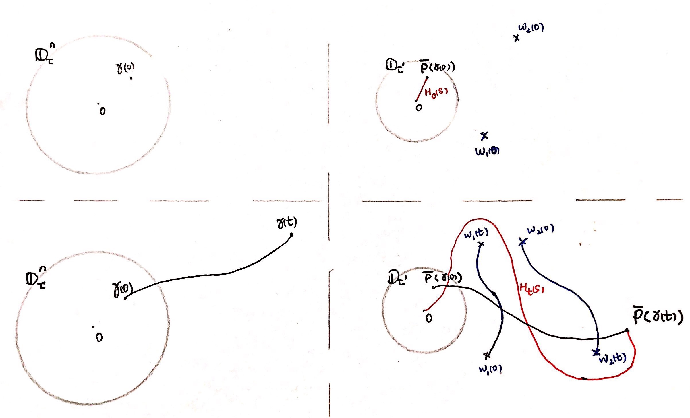
Figure 1: Upper-left: there exists some $\tau$ s.t. $f$ holomorphic in $\mathbb{D}_{\tau}^{n}$ and $f$ continued analytically start at $\gamma(0)$. Upper-right: Integrate $F$ over a line segment $H_{0}(s)$ contained in $\mathbb{D}_{\tau^{\prime}}$. And when $f$ continued analytically along $\gamma(t)$ in the lower-left picture, the corresponding homotopy $H_{t}(s)$(red curve in lower-right) always exists cause the conditions (5.11).

To find the $\gamma$-homotopy is sufficient to find the injective maps $\Psi_{t}:\mathbb{C}\times\mathbb{R}\rightarrow\mathbb{C}\times\mathbb{R}$ satisfies the following conditions: 

$$\begin{split}&(1^{\circ}):\Psi_{0}=id;\\ &(2^{\circ}):\Psi_{t}(0,0)=(0,0);\\ &(3^{\circ}):\Psi_{t}(\omega_{0}(0),0)=(\omega_{0}(t),\mathfrak{L}_{\omega_{0}(t)}),\text{ where }\mathfrak{L}_{\omega_{0}(t)}:=\int_{0}^{t}|\omega_{0}^{\prime}(s)|ds.\\ &(4^{\circ}):\Psi_{t}(\omega_{i}(0),\lambda)=(\omega_{i}(t),\lambda+\mathfrak{L}_{\omega_{i}(t)}),\text{ for }i=1,\cdots,M.\end{split}$$ (5.12)

Indeed, the maps $\Psi_{t}$ will be generated by the flow of a non-autonomous vector field $(X(\xi,\lambda,t),|X(\xi,\lambda,t)|)$ defined as follows:

$$X(\xi,\lambda,t)=\sum\limits_{i=0}^{N}\frac{N_{i}(\xi,\lambda,t)}{N_{i}(\xi,\lambda,t)+\eta_{i}(\xi,\lambda,t)}(\omega_{i}^{\prime}(t),|\omega_{i}^{\prime}(t)|),$$

where

$$\begin{split}&N_{0}(\xi,\lambda,t):=dist((\xi,\lambda),(S(t),\mathbb{R})\cup\{(0,0)\});\\ &N_{i}(\xi,\lambda,t):=dist((\xi,\lambda),(S_{i}(t),\mathbb{R})\cup\{(0,0)\}\cup\{(\omega_{0}(t),\mathfrak{L}_{\omega_{0}(t)})\})\ \text{for}\ i=1,\cdots,N;\\ &\eta_{0}(\xi,\lambda,t):=dist((\xi,\lambda),(\omega_{0}(t),\mathfrak{L}_{\omega_{0}(t)}));\\ &\eta_{i}(\xi,\lambda,t):=|\xi-\omega_{i}(t)|,\ \text{for}\ i=1,\cdots,N;\\ &S(t):=\{\omega_{1}(t),\cdots,\omega_{n}(t)\};\\ &S_{i}(t):=S(t)-\{\omega_{i}(t)\}.\end{split}$$

One can check $N_{i}+\eta_{i}\neq 0$ for $i=1,\cdots,N$. The Cauchy-Lipschitz theorem on the existence and uniqueness of solutions to differential equations applies to $\frac{(d\xi,d\lambda)}{dt}=(X(\xi,\lambda,t),|X(\xi,\lambda,t)|)$: for every $(\xi,\lambda)\in\mathbb{C}\times\mathbb{R}$ and $t_{0}\in[0,1]$ there is a unique solution $t\mapsto\Psi^{t_{0},t}(\xi,\lambda)$ such that $\Psi^{t_{0},t_{0}}=id$. 
Let us set $t_{0}=0$ and $\Psi_{t}:=\Psi^{0,t}$ for $t\in[0,1]$. It is easy to see that this family of maps are injective and satisfy the conditions(5.12) of $\Psi$. We conclude the proof of lemma 5.2 in case 1.  

Here are two simple examples in case 1.

Example 5.6.

$f(z,z_{2}):=\int_{0}^{z}\frac{1}{z_{2}z_{1}+1}dz_{1}=\frac{1}{z_{2}}log(z_{2}z+1)$. One can find multi-path in $\mathbb{C}^{2}$ to prove that the singular set of $f$ is $\{(z,z_{2})\mid z_{2}(z_{2}z+1)=0\}$. And $\{z_{2}=0\}$ is actually the first condition in (5.6), $\{z_{2}z+1=0\}$ is the fourth condition.

Example 5.7.

$f(z,z_{2}):=\int_{0}^{z}\frac{1}{(z_{1}+1)(z_{1}+z_{2}+1)}dz_{1}=\frac{1}{z_{2}}(log(z+1)-log(z+z_{2}+1)+log(z_{2}+1))$. The singular set of $f$ is $\{(z,z_{2})\mid z_{2}(z+1)(z+z_{2}+1)(z_{2}+1)=0\}$. $\{z_{2}=0\}$ is actually the third condition in (5.6), $\{(z+1)(z+z_{2}+1)=0\}$ is the fourth condition, And $\{z_{2}+1=0\}$ is the second condition.

Remark 5.8.

Although the definition $V_{f}^{J}$ gives the possibly singular set, which means that maybe a subset of $V_{f}^{J}$ is regular, from these two simple examples, one can observe that all the conditions in (5.6) make sense.

Now we discuss the lemma 5.2 in case 2. The following example helps us to understand how case 2 happens.

Example 5.9.

If

$$f(z,z_{2}):=\int_{0}^{z_{2}}\frac{1}{z_{2}-z_{1}}log(1-(z_{2}-z_{1}))dz_{1},$$

we know $F(z_{1},z_{2}):=\frac{1}{z_{2}-z_{1}}log(1-(z_{2}-z_{1}))$ is holomorphic at $(0,0)$ and it has singular set $V_{f}=\{(z_{1},z_{2})\mid(z_{1}-z_{2})(z_{1}-(z_{2}-1))=0\}$. Thus $\omega_{1}=z_{2}=\overline{P}$, $\omega_{2}=z_{2}-1$. After change the variable $u=z_{2}-z_{1}$, we have

$$f(z,z_{2})=\int_{0}^{z_{2}}\frac{1}{u}log(1-u)du=-\operatorname{Li}_{2}(z_{2}).$$ (5.13)

It is obvious that the singular set of $f$ is $\{z_{2}=0,1\}$ if we compute partial derivative $\frac{\partial f}{\partial z_{2}}$.

We will use the following homotopy in case 2:

Definition 5.10.

For a multi-path $\gamma(t):=(\gamma_{z}(t),\gamma_{z_{2}}(t),\cdots,\gamma_{z_{n}}(t))\in\mathbb{C}^{n}$, a continuous map $H:[0,1]\times[0,1]\rightarrow\mathbb{C},(t,s)\mapsto H_{t}(s):=H(t,s)$ is called a $\gamma^{\prime}$-homotopy if for any $t\in[0,1]$,

$$\begin{split}&H_{t}(0)=0;\quad H_{0}(s)=s\cdot\overline{P}(\gamma(0))\ \forall s\in[0,1];\quad H_{t}(1)=\overline{P}(\gamma(t));\\ &P_{F}^{J}(H_{t}(s),\gamma_{z_{2}}(t),\cdots,\gamma_{z_{n}}(t))\neq 0\ \forall s\in[0,1).\end{split}$$ (5.14)

In order to prove lemma 5.2, we will use the same procedure as in case 1. We shall use the same formula (5.9) to write down the analytic continuation of $f$ along $\gamma(t)$. The only difference between $\gamma^{\prime}$-homotopy and $\gamma$-homotopy is the ending points (when $s=1$) of the fourth condition in (5.8) and (5.14). Thus we shall prove the germs

$$\left(cont_{(H|_{t}(1),\gamma_{z_{2}}|_{t},\cdots,\gamma_{z_{n}}|_{t})}F\right)(z_{1},\cdots,z_{n})$$

inside integral representation (5.9) are well-defined.

Let $\omega_{i}(t):=\omega_{i}(\gamma_{z_{2}}(t),\cdots,\gamma_{z_{n}}(t))\in\mathbb{C},\ \text{for }i=1,\cdots,M\text{ and }\overline{P}(\gamma(t))=\omega_{1}(t).$

Actually, $\omega_{1}(t)$ is not a singular point for $\gamma^{\prime}$-homotopy because variable ($z_{1}-\overline{P}$) always lies in the principle sheet when we move along $\gamma$. It will be clear after we change the variable:

$$f(z,z_{2},\cdots,z_{n})=\overline{P}(z,z_{2},\cdots,z_{n})\int_{-1}^{0}G(\zeta,z_{2},\cdots,z_{n})d\zeta$$

with $G(\zeta,z_{2},\cdots,z_{n}):=F\left(\overline{P}(z,z_{2},\cdots,z_{n})(1+\zeta),z_{2},\cdots,z_{n}\right)$. We can find sufficient small $R>0$ s.t.

$$G(\zeta,z_{2},\cdots,z_{n})=\frac{1}{2\pi i}\oint_{\partial\mathbb{D}_{R}}\frac{G(\xi,z_{2},\cdots,z_{n})}{\xi-\zeta}d\xi.$$

Indeed, the set (5.5) which $\gamma(t)$ should avoid implies that the moving singular points of $G$

$$\eta_{i}(t):=\frac{\omega_{i}(t)}{\omega_{1}(t)}-1,\quad\text{for}\ i=2,\cdots,M$$

never touch $0$. This allows us to choose sufficient small $R$ s.t. $\eta_{i}(t)$ always lie outside $\mathbb{D}_{R}$. One can prove that such $G$ always holomorphic at $(0,\gamma_{z_{2}}(t),\cdots,\gamma_{z_{n}}(t))$. We conclude the proof of lemma 5.2 in case 2. 

Proof of lemma 3.5.

Given $\overline{P}(z_{2},\cdots,z_{n})\in\mathbb{C}[z_{2},\cdots,z_{n}]$, we may apply lemma 3.4 treating $\overline{P}$ as an element of $\mathbb{C}[z_{1},\cdots,z_{n}]$: $f(z_{2},\cdots,z_{n})=g(z,z_{2},\cdots,z_{n})$ with $g\in\widehat{\mathcal{Q}}^{\mathcal{A}}_{n}$. We observe that formulas (5.6) and (5.7) yield $V_{g}=\mathbb{C}\times V_{f}$, hence $f\in\widehat{\mathcal{Q}}^{\mathcal{A}}_{n-1}$. ∎

6 Hadamard Product

6.1 Introduction to Hadamard product on $\mathbb{C}$

In this section, we study the analytic continuation of the Hadamard product.

Definition 6.1.

Let $f(\xi),g(\xi)\in\mathbb{C}[[\xi]]$, $f(\xi)=\sum\limits_{n=0}^{\infty}a_{n}\xi^{n}$, $g(\xi)=\sum\limits_{m=0}^{\infty}b_{m}\xi^{m}$, we define Hadamard product:

$$f\odot g(\xi)=\sum\limits_{n=0}^{\infty}a_{n}b_{n}\xi^{n}.$$

A fact is that if $f,g\in\mathbb{C}\{\xi\}$, i.e. $f$ and $g$ have positive radius of convergence $R_{f}$ and $R_{g}$ correspondingly, then $f\odot g\in\mathbb{C}\{\xi\}$ and $R_{f\odot g}\leq R_{f}R_{g}$. The following theorem is related to the classical “Hadamard multiplication theorem”, and is in fact a weaker version of a theorem proved in [LSS20].

Theorem E.

If $f,g\in\widehat{\mathcal{Q}}^{\mathcal{A}}_{1}$, which means, $f,g\in\mathbb{C}\{\xi\}$ and they admit analytic continuation along any path which avoids finite points sets $S_{f}$ and $S_{g}$ correspondingly, then $f\odot g\in\widehat{\mathcal{Q}}^{\mathcal{A}}_{1}$ and it admits analytic continuation along any path which starts near origin and avoids $\{0\}\cup S_{f}\cdot S_{g}$.

We may give a sketch of our proof. Choose $\xi$ inside $\mathbb{D}(R_{f}R_{g}):=\{z\in\mathbb{C}\mid|z|<R_{f}R_{g}\}$ and choose $c>0$ s.t.

$$\frac{|\xi|}{\delta_{g}}<c<\delta_{f},$$

we have the integration representation of Hadamard product:

$$f\odot g(\xi)=\frac{1}{2\pi i}\oint_{C}f(z)g(\frac{\xi}{z})\frac{dz}{z},$$ (6.1)

where $C$ is a circle which can be parametrized by $ce^{is},0\leqslant s\leqslant 2\pi.$ 

Example 6.2.

If $f(\xi)=log(1-\xi)$, then one can compute

$$\frac{d}{d\xi}(f\odot f)(\xi)=-\frac{1}{\xi}log(1-\xi),$$

which means the singular points of $f\odot f$ are $0$ and $1$. In fact $f\odot f=\operatorname{Li}_{2}$ as in (2.10).

In order to prove the theorem E, we shall use the following homotopy:

Definition 6.3.

$\gamma^{C}$-homotopy for $1$ dimension case is a continuous map $H:(t,s)\in[0,1]\times[0,2\pi]\rightarrow H_{t}(s)\in\mathbb{C}$ such that:

$$H_{0}(s)=ce^{is},\ \ H_{t}(s)\neq 0,\ \ H_{t}(s)\cap S_{f}=\emptyset,\ \ \frac{\gamma(t)}{H_{t}(s)}\cap S_{g}=\emptyset.$$

Claim 6.4.

If there exists a $\gamma^{C}$-homotopy, then we can do analytic continuation in the following way:

$$(cont_{\gamma|_{t}}f\odot g)(\xi)=\frac{1}{2\pi i}\oint_{H_{t}}(cont_{H_{|t}(s)}f)(z)(cont_{\frac{\gamma|_{t}}{H_{|t}(s)}}g)({\frac{\xi}{z}})\frac{dz}{z}.$$ (6.2)

Proof.

Similar to the proof of claim 5.4. ∎

Claim 6.5.

If $\gamma$ starts near origin and it avoids $\{0\}\cup S_{f}\cdot S_{g}$, then there exists $\gamma^{C}$-homotopy.

Proof.

Suppose $S_{f}=\{f_{1},\cdots,f_{s}\}$, $S_{g}=\{g_{1},\cdots,g_{r}\}$. Without loss of generality, we assume $g_{i}\neq 0$ for all $i=1,\cdots,r$. Indeed, if $g_{1}=0$, it has no influence on the $\gamma^{C}$-homotopy because $\gamma(t)$ never touch $0$. Let

$$\omega_{i}(t)=\frac{\gamma(t)}{g_{i}},\indent i=1,\cdots,r,$$

be the moving singular points of homotopy. By the assumption, $\gamma(t)\neq 0$ implies that $\omega_{i}(t)\neq\omega_{j}(t)$ for $i\neq j$ and $\omega_{i}(t)\neq 0$, $\gamma(t)\neq S_{f}\cdot S_{g}$ implies that $\omega_{j}(t)\neq f_{i}$.  

To find the homotopy is sufficient to find the flow $\Psi_{t}:\mathbb{C}\rightarrow\mathbb{C}$ which satisfies: 

$$\begin{split}&\Psi_{0}=id,\\ &\Psi_{t}(0)=0,\\ &\Psi_{t}(f_{i})=f_{i}\text{\indent for }i=1,\cdots,s,\\ &\Psi_{t}(\omega_{j}(0))=\omega_{j}(t)\text{\indent for }j=1,\cdots,r.\end{split}$$

See the picture below.

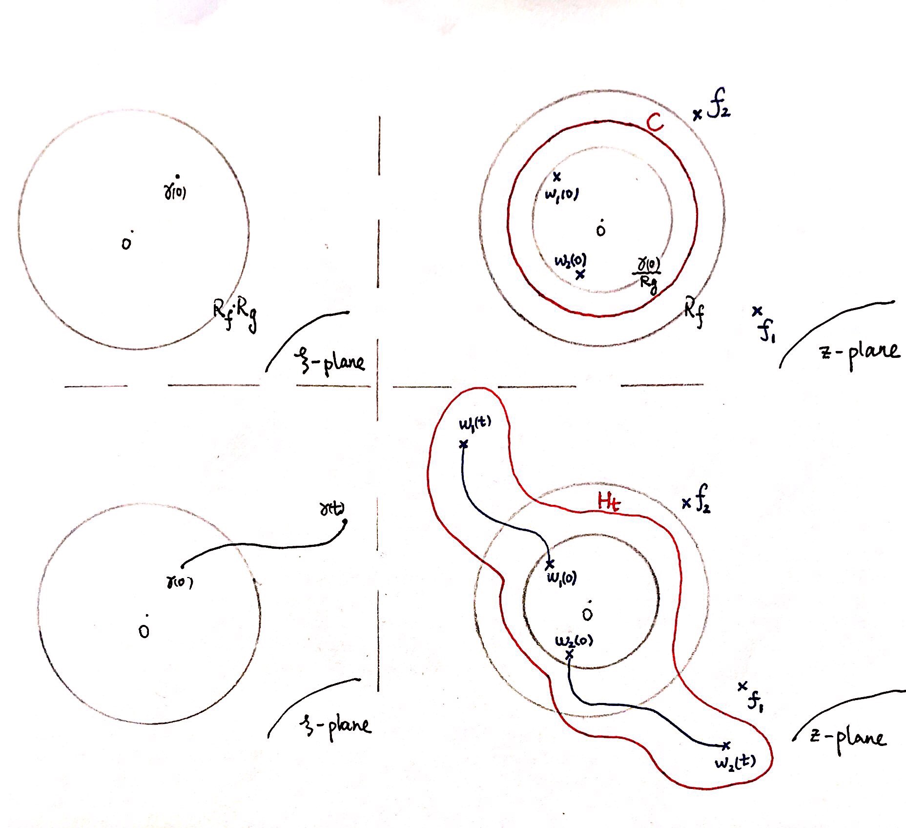
Figure 2: Upper-left: $f\odot g$ is holomorphic in $\mathbb{D}_{R_{f}\cdot R_{g}}$ and $f$ continued analytically start at $\gamma(0)\in\mathbb{D}_{R_{f}\cdot R_{g}}$. Upper-right: Using $C$ to be the integral curve when $t=0$, we notice that the singular points of $f$ are outside $\mathbb{D}_{R_{f}\cdot R_{g}}$ and the “moving singular points” of the homotopy are inside $\mathbb{D}_{R_{f}\cdot R_{g}}$. And when $f\odot g$ continued analytically along $\gamma(t)$ in the lower-left picture, the corresponding homotopy $H_{t}(s)$(red curve in lower-right) always exists cause the conditions of $\omega(t)$’s.

Then we shall use the non-autonomous vector field:

$$X(\xi,t)=\sum\limits_{i=1}^{r}\frac{\eta_{i}(\xi,t)}{\eta_{i}(\xi,t)+\tau_{i}(\xi,t)}\omega_{i}^{\prime}(t)$$

$$\text{with}\quad\eta_{i}(\xi,t):=dist\left(\xi,\{0\}\cup S_{f}\cup\bigcup\limits_{i\neq j}\omega_{j}(t)\right)\quad\text{and}\quad\tau_{i}(\xi,t):=dist(\xi,\omega_{i}(t)).$$

The Cauchy-Lipschitz theorem on the existence and uniqueness of solutions to differential equations applies to $\frac{d\xi}{dt}=X(\xi,t)$: for every $\xi\in\mathbb{C}$ and $t_{0}\in[0,1]$ there is a unique solution $t\rightarrow\Phi^{t_{0},t}(\xi)$ such that $\Phi^{t_{0},t_{0}}(\xi)=\xi$. Then we shall define our flow $\Psi_{t}=\Phi^{0,t}$ for $t\in[0,1]$ and the $\gamma^{C}$-homotopy $H_{t}(s):=\Phi_{t}(H_{0}(s))$. ∎

6.2 Proof of lemma 3.3

Suppose $\hat{f}(\xi,q,p),\hat{g}(\xi,q,p)\in\widehat{\mathcal{Q}}^{\mathcal{A}}_{3}$, which means $\hat{f},\hat{g}$ holomorphic at $\mathbb{D}^{3}(\tau,0)$ and the avoidant algebraic sets are

$$\begin{split}V_{f}:=\bigcap\limits_{J=1}^{R}V_{f}^{J},&\quad V_{f}^{J}:=\{(\xi,q,p)\in\mathbb{C}^{3}\mid P_{f}^{J}(\xi,q,p)=0\},\text{ for }J=1,\cdots,R,\\ V_{g}:=\bigcap\limits_{K=1}^{S}V_{g}^{K},&\quad V_{g}^{K}:=\{(\xi,q,p)\in\mathbb{C}^{3}\mid Q_{g}^{K}(\xi,q,p)=0\},\text{ for }K=1,\cdots,S,\end{split}$$

correspondingly, with $P_{f}^{J}$’s are $p$-simple polynomials and $Q_{g}^{K}$’s are $q$-simple polynomials.  

For each $J=1,\cdots,R,K=1,\cdots,S$, we shall construct algebraic variety $V_{F}^{JK}$, s.t. if $f$ avoids the set $\{x\in\mathbb{C}^{n}\mid x\in{(P_{f}^{J})}^{-1}(0)\}$, and $g$ avoids the set $\{x\in\mathbb{C}^{n}\mid x\in{(Q_{g}^{K})}^{-1}(0)\}$, then $F$ admits analytic continuation along any $\gamma$ which avoids the set $V_{F}^{JK}$. Thus finally, the avoidant set of $F$ is an algebraic variety

$$V_{F}=\bigcap\limits_{J,K}V_{F}^{JK}.$$

For simplifying the notation, let

$$\begin{split}&P_{f}^{J}(\xi,q,p)=a_{M}(\xi,q)\prod\limits_{\alpha=1}^{M}\big{(}p-\widetilde{\omega}_{\alpha}(\xi,q)\big{)},\\ &Q_{g}^{K}(\xi,q,p)=b_{N}(\xi,p)\prod\limits_{\beta=1}^{N}\big{(}q-\widetilde{\Omega}_{\beta}(\xi,p)\big{)},\end{split}$$ (6.3)

with $a_{M},b_{N}\neq 0$, $\widetilde{\omega}_{\alpha_{1}}\neq\widetilde{\omega}_{\alpha_{2}}$ if $1\leq\alpha_{1}<\alpha_{2}\leq M$, $\widetilde{\Omega}_{\beta_{1}}\neq\widetilde{\Omega}_{\beta_{2}}$ if $1\leq\beta_{1}<\beta_{2}\leq N$, just like what we do in section 5. We shall keep in mind that the notations $a_{M}$, $M$, and $\widetilde{\omega}_{\alpha}$’s are depend on $J$, and $b_{N}$, $N$, and $\widetilde{\Omega}_{\beta}$’s are depend on $K$.

By the formula (3.4), one can easily prove that $F$ is holomorphic inside $\mathbb{D}(\tau)\times\mathbb{D}(\tau)\times\mathbb{D}(\frac{\tau^{2}}{4})\times\mathbb{D}(\frac{\tau}{2})\times\mathbb{D}(\frac{\tau}{2})$. We shall choose a point $(\xi_{1},\xi_{2},\xi_{3},q,p)$ in this polydisc, then there exists $c>0$, s.t.

$$\frac{|\xi_{3}|}{\frac{\tau}{2}}<c<\frac{\tau}{2}.$$

The formula (3.4) is equivalent to

$$F(\xi_{1},\xi_{2},\xi_{3},q,p)=\frac{1}{2\pi i}\oint_{C}f(\xi_{1},q,p+z)g(\xi_{2},q+\frac{\xi_{3}}{z},p)\frac{dz}{z}$$ (6.4)

where $C$ is a circle radius $c$, center at origin. 
Let us consider the polynomials

$$\begin{split}&P_{f}^{J}(\xi_{1},q,p+z):=a_{M}(\xi_{1},q)\prod\limits_{\alpha=1}^{M}(z-\omega_{\alpha}(\xi_{1},q,p))\in\mathbb{C}[\xi_{1},q,p,z],\\ &Q_{g}^{K}(\xi_{2},q+z,p):=b_{N}(\xi_{2},p)\prod\limits_{\beta=1}^{N}(z-\Omega_{\beta}(\xi_{2},q,p))\in\mathbb{C}[\xi_{2},q,p,z].\end{split}$$ (6.5)

From the lemma 4.3, we know that these two polynomials are both $z$-simple polynomials, which means that we have

$$\begin{split}&a_{M}\neq 0,\quad\omega_{\alpha_{1}}\neq\omega_{\alpha_{2}}\text{ if }1\leq\alpha_{1}<\alpha_{2}\leq M,\\ &b_{N}\neq 0,\quad\Omega_{\beta_{1}}\neq\Omega_{\beta_{2}}\text{ if }1\leq\beta_{1}<\beta_{2}\leq N.\end{split}$$ (6.6)

We shall define the avoidant set of $F$ in $\mathbb{C}^{5}$ by using the notations above. One may notice that it is a ‘symmetry’ condition:  

Definition 6.6.

$$V_{F}^{JK}:=\mathbb{C}^{5}-\left\{(\xi_{1},\xi_{2},\xi_{3},q,p)\in\mathbb{C}^{5}\left|\begin{split}&\mathfrak{P}_{\xi_{1},q,p}(z)\text{ has }M\text{ distinct non-zero roots,\ and}\\ &\mathfrak{Q}_{\xi_{2},q,p}(z)\text{ has }N\text{ distinct non-zero roots,\ and}\\ &\xi_{3}\notin\{\omega_{\alpha}\Omega_{\beta}\}\cup\{0\}\end{split}\right.\right\},$$

where $\mathfrak{P}_{\xi_{1},q,p}(z):=P_{f}^{J}(\xi_{1},q,p+z)$ is treated as a polynomial of one variable $z$ with the coefficients in $\mathbb{C}[\xi_{1},q,p]$ and $\mathfrak{Q}_{\xi_{2},q,p}(z):=Q_{g}^{K}(\xi_{2},q+z,p)$ is treated as a polynomial of one variable $z$ with the coefficients in $\mathbb{C}[\xi_{2},q,p]$.

Remark 6.7.

In fact, $V_{F}^{JK}$ will be simplified to one sentence:

$$V_{F}^{JK}=\mathbb{C}^{5}-\left\{(\xi_{1},\xi_{2},\xi_{3},q,p)\in\mathbb{C}^{5}\left|z^{N}\mathfrak{P}_{\xi_{1},q,p}(z)\mathfrak{Q}_{\xi_{2},q,p}(\frac{\xi_{3}}{z})\text{ has $M+N$ distinct non-zero roots}\right.\right\}.$$ (6.7)

By the lemma 4.4, we know $V_{F}^{JK}$ is an algebraic variety.

From the discussion above, to prove the lemma 3.3 is sufficient to prove the following claim:

Claim 6.8.

If $f$ and $g$ admit analytic continuation along any path which avoid $V_{f}^{J}$ and $V_{g}^{K}$ respectively, then $F$ defined by formula (6.4) admits analytic continuation along any path $\gamma$ which avoids $V_{F}^{JK}$ defined above.

By using following seven conditions, we explain $V_{F}^{JK}$ more precisely,

$$V_{F}^{JK}=\left\{(\xi_{1},\xi_{2},\xi_{3},q,p)\in\mathbb{C}^{5}\left|\begin{split}&a_{M}(\xi_{1},q)=0&\text{ or }&\\ &b_{N}(\xi_{2},p)=0&\text{ or }&\\ &\omega_{\alpha_{1}}(\xi_{1},q,p)=\omega_{\alpha_{2}}(\xi_{1},q,p)\text{ for }\alpha_{1}\neq\alpha_{2}&\text{ or }&\\ &\Omega_{\beta_{1}}(\xi_{2},q,p)=\Omega_{\beta_{2}}(\xi_{2},q,p)\text{ for }\beta_{1}\neq\beta_{2}&\text{ or }&\\ &\omega_{\alpha}(\xi_{1},q,p)=\frac{\xi_{3}}{\Omega_{\beta}(\xi_{2},q,p)}&\text{ or }&\\ &\omega_{\alpha}(\xi_{1},q,p)=0&\text{ or }&\\ &\xi_{3}=0\end{split}\right.\right\}$$ (6.8)

where $\alpha,\alpha_{1},\alpha_{2}=1,\cdots,M$ and $\beta,\beta_{1},\beta_{2}=1,\cdots,N$.

We assume $\gamma:[0,1]\rightarrow\mathbb{C}^{5}$ starting near $0\in\mathbb{C}^{5}$, denoted by $\gamma(t)=(\gamma_{\xi_{1}}(t),\gamma_{\xi_{2}}(t),\gamma_{\xi_{3}}(t),\gamma_{q}(t),\gamma_{p}(t))$. We shall use the following homotopy to do analytic continuation:

Definition 6.9.

With a little abuse of name, a $\gamma^{C}$-homotopy for high dimension is a continuous map $H:(t,s)\in[0,1]\times[0,2\pi]\rightarrow H_{t}(s)\in\mathbb{C}$ s.t. for any $t,s,\alpha,\beta$:

$$H_{0}(s)=ce^{is},\quad H_{t}(s)\neq 0,\quad H_{t}(s)\neq\omega_{\alpha}(\xi_{1},q,p),\quad H_{t}(s)\neq\frac{\xi_{3}}{\Omega_{\beta}(\xi_{2},q,p)}.$$

One shall prove that if there exists such $\gamma^{C}$-homotopy, then

$$\begin{split}(cont_{\gamma|_{t}}F)(\xi_{1},\xi_{2},\xi_{3},q,p)=\frac{1}{2\pi i}\oint_{H_{t}}\left(cont_{(\gamma_{\xi}|_{t},\gamma_{q}|_{t},\gamma_{p}|_{t}+H|_{t}(s))}\hat{f}\right)(\xi_{1},q,p+z)\\ \cdot\left(cont_{(\gamma_{\xi_{2}}|_{t},\gamma_{q}|_{t}+\frac{\gamma_{\xi_{3}}|_{t}}{H|_{t}(s)},\gamma_{p}|_{t})}\hat{g}\right)(\xi_{2},q+\frac{\xi_{3}}{z},p)\frac{dz}{z},\end{split}$$

which means $F$ admits analytic continuation along $\gamma$ (see the proof of claim 5.4 for details). 

Now we assume $\gamma$ avoids $V_{F}^{JK}$, to find the homotopy is sufficient to find the flow $\Psi_{t}:\mathbb{C}\rightarrow\mathbb{C}$ which satisfies: 

$$\begin{split}&\Psi_{0}=id,\\ &\Psi_{t}(0)=0,\\ &\Psi_{t}(\omega_{i})=\omega_{i}(t)\text{\indent for }i=1,\cdots,N+M,\end{split}$$

where $\omega_{N+j}(t):=\frac{\xi_{3}}{\Omega_{j}(t)}$, $j=1,\cdots,M$. Here we use $\omega_{\alpha}(t)$ and $\Omega_{\beta}(t)$ to simplify the notation $\omega_{\alpha}(\gamma_{\xi_{1}}(t),\gamma_{q}(t),\gamma_{p}(t))$ and $\Omega_{\beta}(\gamma_{\xi_{2}}(t),\gamma_{q}(t),\gamma_{p}(t))$ respectively.  

From the third condition to last condition in definition (6.8), we know that if $\gamma$ avoids $V_{F}^{JK}$, then $\omega_{i}(t)\neq\omega_{j}(t)$ and $\omega_{i}(t)\neq 0$ for $1\leq i\neq j\leq M+N$. The first two conditions in definition (6.8) provide that no moving singular points goes to infinity.

Thus we could use the non-autonomous vector field:

$$X(\xi,t)=\sum\limits_{i=1}^{r}\frac{\eta_{i}(\xi,t)}{\eta_{i}(\xi,t)+\tau_{i}(\xi,t)}\omega_{i}^{\prime}(t)$$

where $\eta_{i}(\xi,t):=dist(\xi,\{0\}\cup\bigcup\limits_{j\neq i}\omega_{j}(t))$ and $\tau_{i}(\xi,t):=dist(\xi,\omega_{i}(t))$. The Cauchy-Lipschitz theorem on the existence and uniqueness of solutions to differential equations applies to $\frac{d\xi}{dt}=X(\xi,t)$: for every $\xi\in\mathbb{C}$ and $t_{0}\in[0,1]$ there is a unique solution $t\rightarrow\Phi^{t_{0},t}(\xi)$ such that $\Phi^{t_{0},t_{0}}(\xi)=\xi$. Then we shall define our flow $\Psi_{t}=\Phi^{0,t}$ for $t\in[0,1]$ and the desired $\gamma^{C}$-homotopy $H_{t}(s):=\Psi_{t}(ce^{is})$. We conclude the proof of claim 6.8. 

Example 6.10.

Let $f(\xi,q,p)=log(3-\xi-q-p)$ and $g(\xi,q,p)=\frac{1}{3-\xi-q-p}\cdot\frac{1}{4-\xi-2q-p}$, thus $f$ and $g$ holomorphic in $\mathbb{D}(1)\times\mathbb{D}(1)\times\mathbb{D}(1)$. From the discussion above, we know $F$ holomorphic in $\mathbb{D}(1)\times\mathbb{D}(1)\times\mathbb{D}(\frac{1}{4})\times\mathbb{D}(\frac{1}{2})\times\mathbb{D}(\frac{1}{2})$. 
We choose $\gamma_{\xi_{3}}(0)=\frac{1}{8}$, then there exists $c>0$ (we may choose $c=\frac{3}{8}$) s.t. $\frac{\frac{1}{8}}{\frac{1}{2}}<c<\frac{1}{2}$. From the formula (6.4), we compute

$$\begin{split}F(\xi_{1},\xi_{2},\xi_{3},q,p)&=\frac{1}{2\pi i}\oint_{C}log(3-\xi_{1}-q-p-z)\cdot\frac{1}{3-\xi_{2}-q-\frac{\xi_{3}}{z}-p}\cdot\frac{1}{4-\xi_{2}-2q-\frac{2\xi_{3}}{z}-p}\frac{dz}{z}\\ &=\frac{1}{A}\frac{1}{B}\frac{1}{2\pi i}\oint_{C}\frac{1}{z-\frac{\xi_{3}}{A}}\cdot\frac{1}{z-\frac{2\xi_{3}}{B}}\cdot zdz\\ &=\left[log(3-\xi_{1}-q-p-\frac{\xi_{3}}{A})\cdot\frac{\xi_{3}}{A}-log(3-\xi_{1}-q-p-\frac{2\xi_{3}}{B})\cdot\frac{2\xi_{3}}{B}\right]\cdot\frac{1}{\xi_{3}(B-2A)}\\ &=\frac{1}{\xi_{2}+p-2}\cdot\Big{[}log(3-\xi_{1}-q-p-\frac{\xi_{3}}{A})\cdot\frac{1}{A}-log(3-\xi_{1}-q-p-\frac{2\xi_{3}}{B})\cdot\frac{2}{B}\Big{]},\end{split}$$

where $A:=3-\xi_{2}-q-p$ and $B:=4-\xi_{2}-2q-p$. Here we know $P_{f}(\xi_{1},q,p)=1$, $P_{g}(\xi_{2},\xi_{3},q,p)=AB$, $\omega_{1}=3-\xi_{1}-q-p$, $\Omega_{1}=\frac{\xi_{3}}{A}$, $\Omega_{2}=\frac{2\xi_{3}}{B}$. Thus we can easily observe that $F$ has singular set when $A=0,B=0,\omega_{1}=\Omega_{1},\omega_{1}=\Omega_{2},\Omega_{1}=\Omega_{2}$. In fact, for the case $\Omega_{1}=\Omega_{2}$, which means $\xi_{2}+p-2=0$, is not singular set at principle sheet of germ $F$, but it may be singular set in some other sheet.  

Remark 6.11.

The above computation gives an example for the second, fourth and fifth condition in definition (6.8). One may find examples for other conditions.

7 Conclusion of the proof for an arbitrary number of degrees of fredom

Now we assume $q=(q_{1},\cdots,q_{r})$ and $p=(p_{1},\cdots,p_{r})$. Recall the integral formula (2.20):

$$\begin{split}\hat{f}\ast\hat{g}(\xi,q,p)=&\frac{d^{r+2}}{d\xi^{r+2}}\int^{\xi}_{0}d\xi_{1}\int^{\xi-\xi_{1}}_{0}d\xi_{2}\cdots\int_{0}^{\xi-\xi_{1}-\cdots-\xi_{r+1}}d\xi_{r+2}\big{(}\frac{1}{2\pi}\big{)}^{r}\overbrace{\int_{0}^{2\pi}\cdots\int_{0}^{2\pi}}^{r}d\theta_{1}\cdots d\theta_{r}\\ &\hat{f}(\xi_{r+1},q_{1},\cdots,q_{r},p_{1}+\sqrt{\xi_{1}}e^{-i\theta_{1}},\cdots,p_{r}+\sqrt{\xi_{r}}e^{-i\theta_{r}})\\ &\hat{g}(\xi_{r+2},q_{1}+\sqrt{\xi_{1}}e^{i\theta_{1}},\cdots,q_{r}+\sqrt{\xi_{r}}e^{i\theta_{r}},p_{1},\cdots,p_{r}).\end{split}$$

We want to prove Theorem B, i.e. that $\hat{f},\hat{g}\in\mathcal{Q}^{\mathcal{A}}_{2r+1}\enspace\Longrightarrow\enspace\hat{f}\ast\hat{g}\in\mathcal{Q}^{\mathcal{A}}_{2r+1}$.

Then, by using our lemmas on convolution product and Hadamard product, we will be able to deduce the same result for $*_{M}$, i.e. Theorem A, because

$$\hat{f}\in\widehat{\mathcal{Q}}^{\mathcal{A}}_{2r+1}\enspace\Longrightarrow\enspace\widehat{T}\hat{f}\in\widehat{\mathcal{Q}}^{\mathcal{A}}_{2r+1}$$ (7.1)

by the same arguments as below.

The following definition is useful.

Definition 7.1.

For $n\geq 2$, $i\leq j\leq n$,

$$F(z_{1},\cdots,z_{n})\in\mathbb{C}\{z_{1},\cdots,z_{n}\}\mapsto(\odot_{ij}F)(\xi,z_{1},\cdots,z_{n})\in\mathbb{C}\{\xi,z_{1},\cdots,z_{n}\},$$

where

$$(\odot_{ij}F)(\xi,z_{1},\cdots,z_{n}):=\int_{0}^{2\pi}F(z_{1},\cdots,z_{i-1},z_{i}+\sqrt{\xi}e^{-i\theta},z_{i+1},\cdots,z_{j-1},z_{j}+\sqrt{\xi}e^{i\theta},z_{j+1},\cdots,z_{n})\frac{d\theta}{2\pi}.$$

By using this definition, we may understand the formula (2.20) as

$$\hat{f}\ast\hat{g}(\xi,q,p)=\frac{d^{r+2}}{d\xi^{r+2}}\int^{\xi}_{0}d\xi_{1}\int^{\xi-\xi_{1}}_{0}d\xi_{2}\cdots\int_{0}^{\xi-\xi_{1}-\cdots-\xi_{r+1}}d\xi_{r+2}G(\xi_{1},\cdots,\xi_{r+2},q,p),$$ (7.2)

where $G$ is obtained by $\odot^{r}_{2r+1,3r+2}(F)$,

$$F(\xi_{1},z_{1},\cdots,z_{2r},\xi_{2},z_{2r+1},\cdots,z_{4r}):=\hat{f}(\xi_{1},z_{1},\cdots,z_{2r})\hat{g}(\xi_{2},z_{2r+1},\cdots,z_{4r})$$

and let $z_{i}=z_{2r+i}=q_{i}$ and $z_{r+j}=z_{3r+j}=p_{j}$ for $i,j=1,\cdots,r$.  

By lemma 3.4 and lemma 3.5, to prove $\hat{f}\ast\hat{g}\in\mathcal{Q}^{\mathcal{A}}_{2r+1}$ is sufficient to prove the following lemma:

Lemma 7.2.

If $F(z_{1},\cdots,z_{n})\in\mathcal{Q}^{\mathcal{A}}_{n}$ then $(\odot_{ij}F)(\xi,z_{1},\cdots,z_{n})\in\mathcal{Q}^{\mathcal{A}}_{n+1}$.

Proof.

We assume $\{(z_{1},\cdots,z_{n})\mid P_{F}(z_{1},\cdots,z_{n})=0\}$ is the avoidant set of $F$. Consider $Q(z,\xi,z_{1},\cdots,z_{n}):=z^{N}P_{F}(z_{1},\cdots,z_{i}+{z},\cdots,z_{j}+\frac{\xi}{z},\cdots,z_{n})$, where $N$ is the smallest number such that $Q$ is a polynomial in the variables $z,\xi,z_{1},\cdots,z_{n}$. We treat $Q_{\xi,z_{1},\cdots,z_{n}}(z):=Q(z,\xi,z_{1},\cdots,z_{n})$ as the polynomial in one variable $z$, order $M$, with coefficient in $\mathbb{C}[\xi,z_{1},\cdots,z_{n}]$. One may prove that, $\odot_{ij}F$ admits analytic continuation along any path which contained in the following set

$$\left\{(\xi,z_{1},\cdots,z_{n})\in\mathbb{C}^{n+1}\left|Q_{\xi,z_{1},\cdots,z_{n}}(z)\text{ has $M$ distinct non-zero roots}\right.\right\}.$$ (7.3)

∎

Acknowledgements

The first and the third authors aknowledge support from NSFC (No.11771303).

The second author thanks Capital Normal University for their hospitality during the period September 2019–February 2020.

The third author is partially supported by NSFC (No.s 11771303, 11911530092, 11871045).

This paper is partly a result of the ERC-SyG project, Recursive and Exact New Quantum Theory (ReNewQuantum) which received funding from the European Research Council (ERC) under the European Union’s Horizon 2020 research and innovation programme under grant agreement No 810573.

References

- [BPP20] P. Banks, E. Panzer and B. Pym, “Multiple zeta values in deformation quantization”, Invent. Math. 222 (2020), no. 1, 79–159.
- [BFFL78] F. Bayen, M. Flato, C. Fronsdal, A. Lichnerowicz and D. Sternheimer, Deformation theory and quantization I, II, Ann. Phys. (NY) 111 (1978) 61–110, 111–151.
- [CNP93] B. Candelpergher, J.-C. Nosmas, and F. Pham. Approche de la résurgence. Actualités Mathématiques. [Current Mathematical Topics]. Hermann, Paris, 1993.
- [DWL83] M. De Wilde and P. Lecomte, “Existence of star-products and of formal deformations of the Poisson Lie algebra of arbitrary symplectic manifolds”, Lett. Math. Phys. 7 (1983), no. 6, 487–496.
- [Dys52] F. J. Dyson, “Divergence of perturbation theory in quantum electrodynamics”, Phys. Rev. 85 (1952) 631–632.
- [Eca81] J. Écalle, Les fonctions résurgentes, Vol. 1. Publ. Math. d’Orsay 81-05, 1981.
- [Eca84] J. Écalle, Cinq applications des fonctions resurgentes, prepublications, Université de Paris-Sud, Orsay, Tome 62, 1984
- [Eca85] J. Écalle, Les fonctions résurgentes, Vol. 3. Publ. Math. d’Orsay 85-05, 1985.
- [Fed85] B. V. Fedosov, Formal quantization. “Some problems in modern mathematics and their applications to problems in mathematical physics” (Russian), 129–136, vi, Moskov. Fiz.-Tekhn. Inst., Moscow, 1985.
- [Fed94] B. V. Fedosov, A simple geometrical construction of deformation quantization, J. Diff. Geom., 40 (1994) 213–238.
- [GGS14] M. Garay, A. de Goursac and D. van Straten, “Resurgent deformation quantisation”, Ann. Physics 342 (2014), 83–102.
- [GKZ94] I. M. Gelfand, M. M. Kapranov and A.V. Zelevinsky, Discriminants, resultants, and multidimensional determinants, Boston: Birkhäuser, 1994, ISBN 978-0-8176-3660-9
- [Kon03] M. Kontsevich, Deformation quantization of Poisson manifolds, q-alg/9709040, Lett. Math. Phys. 66 (2003), no. 3, 157–216.
- [LSS20] Y. Li, D. Sauzin and S. Sun, “Hadamard Product and Resurgence Theory”, preprint 2020, 10 p. [arXiv:2012.14175]
- [Moy49] J. E. Moyal, Quamtum mechanics as a statistical theory, Proc. Cambridge Phil. Soc. 45 (1949), 99–124.
- [Oes98] J. Oesterlé, Quantification formelle des variétés de Poisson, d’aprè M. Kontsevich, Séminaire Bourbaki, 50ème année, 1997–98, n∘ 843.
- [PM20a] R. Pérez-Marco, “Monodromies of singularities of the Hadamard and eñe product” [arXiv:2009.14099v3], 23 p., 2020
-
[PM20b]
R. Pérez-Marco, “Local monodromy formula of
Hadamard products”
[arXiv:2011.10497v1], 18 p., 2020 - [Pha88] F. Pham, Resurgence, quantized canonical transformations, and multi-instanton expansions, Algebraic Analysis (papers dedicated to M. Sato), Vol. II, Academic Press, Boston MA, (1988) 699–726
- [Sau09] D. Sauzin, Mould expansions for the saddle-node and resurgence monomials, in Renormalization and Galois theories, A. Connes, F. Fauvet, J.-P. Ramis (eds.), IRMA Lectures in Mathematics and Theoretical Physics 15, Zürich: European Mathematical Society, 83–163 (2009).
- [Sau13] D. Sauzin, “On the stability under convolution of resurgent functions”, Funkcialaj Ekvacioj Serio Internacia 56, 3 (2013), 397–413. [hal-00656739]
- [Sau15] D. Sauzin, “Nonlinear analysis with resurgent functions”, Annales scientifiques de l’École Normale Supérieure 48, 3 (2015), 667–702. [hal-00766749]
- [MS16] C. Mitschi and D. Sauzin, Divergent Series, Summability and Resurgence. Volume 1: Monodromy and Resurgence. Lecture Notes in Mathematics 2153, Springer, Heidelberg, 2016.
- [Vor83] A. Voros, The return of the quartic oscillator. The complex WKB method, Ann. de l’Institute H. Poincaré, A 39(1983), 211–338
- [Wal00] M. Waldschmidt, “Valeurs zêta multiples. Une introduction”, J. Théor. Nombres Bordeaux 12 (2000), 581–595.
- [Wei94] A. Weinstein, Deformation quantization, Séminaire Bourbaki, exposé no. 789 (juin 1994), Astérique 227, 389–409
- [ZJ83] J. Zinn-Justin, Multi-instanton contributions in quantum mechanics (II), Nuclear Physics B218(1983), 333–348