Towards Colour Flow Evolution at Two Loops

Abstract

We calculate the two-loop and one-loop/one-emission contributions required for soft gluon evolution at the next-to-leading order. The colour structures are expressed in the colour flow basis, and the kinematic dependence and loop integrals are expressed in terms of multiple cuts and phase-space-like integrals. This directly allows to use them in the resummation of non-global observables and improved parton shower algorithms beyond the leading order and beyond the leading colour limit. Within the colour flow basis it becomes apparent that correlations beyond a dipole picture emerge even in colour-diagonal elements of the virtual corrections.

1 Introduction

Precise predictions for collider physics experiments require to include QCD corrections both at fixed-order and within resummed perturbation theory. While fixed-order calculations reliably predict inclusive quantities and the coarse spectra of jets at high transverse momenta, infrared sensitive observables require resummed perturbation theory in order to capture the dominant, logarithmic contributions appearing at each order in the perturbative series. A complementary approach is the use of multi-purpose Monte Carlo event generators, which provide very detailed simulation of realistic final states, including phenomenological models of how a high-multiplicity partonic final state with small inter-parton scales converts into the observed hadrons. The component central to event generators is the parton shower algorithm which describes the evolution from large to small momentum transfers and also facilitates the resummation of large logarithmic contributions.

The resummation of non-global observables Dasgupta:2001sh ; Banfi:2002hw requires a framework of parton evolution at the amplitude level Becher:2016mmh ; Caron-Huot:2015bja ; Martinez:2018ffw , and such a formalism is very promising in providing a theoretical framework which allows to systematically construct parton shower algorithms beyond the currently adopted approximations Nagy:2014mqa ; Forshaw:2019ver , and with the highest level of control over their accuracy. Such a formalism has recently been adopted to make decisive statements about the accuracy of parton showers Forshaw:2020wrq ; Holguin:2020joq ; Dasgupta:2020fwr ; Hamilton:2020rcu ; Nagy:2020rmk . Solving the evolution equations which do resum non-global logarithms requires Monte Carlo methods Balsiger:2018ezi and has recently been extended beyond the leading-$N$ limit Platzer:2013fha ; DeAngelis:2020rvq , addressing a dedicated resummation algorithm before aiming at a more versatile simulation within an event generator. The same formalism also allows to analyze approaches to improve existing parton showers beyond the leading-$N$ limit Platzer:2012np ; Platzer:2018pmd ; Hoeche:2020nsx in order to show which colour suppressed contributions are actually taken into account Holguin:2020oui , highlighting the fact that amplitude level evolution will go beyond a probabilistic approach in the sense that unitarity cannot be naively employed anymore. A connection to colour reconnection models has recently been highlighted, as well Gieseke:2018gff .

In the present work we address key ingredients of extending the amplitude level evolution beyond the leading order, and towards including soft gluon effects at second order in the strong coupling, within the double-soft limit. The evolution at this order will require two-loop, one-loop one-emission and double-emission diagrams to be available in a form appropriate to be handled by a numerical code. This will provide the entry point to include triple-collinear and soft-collinear configurations, and serves the purpose of clarifying the structure of the evolution in colour space similarly to the one-loop anomalous dimension analyzed in Platzer:2013fha . We also establish methodology in order to systematically obtain the virtual corrections required at this order in a representation of phase-space type integrals, which is complementary to approaches which perform the actual integrals and make the divergencies explicit in terms of poles of the dimensional regularisation parameter $\epsilon$, see e.g. results on one-, two- and three-loop divergencies Catani:1996vz ; Catani:1998bh ; Becher:2009cu , as well as the one-loop corrections to the emission of a soft gluon Catani:2000pi . The resulting anomalous dimensions for soft gluon exchange have been discussed in more detail in Aybat:2006wq ; Almelid:2015jia , and their role in resummation of soft gluon effects in hadronic $2\to 2$ scatterings has been pioneered in Kidonakis:1998nf ; Contopanagos:1996nh ; Dokshitzer:2005ig and recently summarised e.g. in Kidonakis:2020gxo . The resummation of soft gluon corrections has also been considered for a larger class than $2\to 2$ scatterings Sjodahl:2008fz , and general algorithms for dealing with the colour structure are available in Sjodahl:2009wx . Our approach focuses on a general algorithm using the colour flow basis, and a formulation appropriate for an arbitrary number of coloured legs. Within our formalism we are also in the position to isolate the imaginary parts of the virtual corrections (which we leave in explicit and detailed form for a future publication), as well as the possibility to straightforwardly implement subtractions, and the evaluation of virtual corrections in a manner inherent to parton branching algorithms based on (weighted) Sudakov veto algorithms Platzer:2011dq ; Bellm:2016voq ; Olsson:2019wvr .

The present work is structured as follows: In Sec. 2 we will first review basic principles of soft gluon evolution in colour space, and in particular at the leading order using one-loop soft exchanges and single emission Eikonal currents. We will also review that the colour structures obtained at this level give rise to a systematic expansion around the leading-$N$ limit. In Sec. 3 we will then perform a detailed analysis of the colour structures encountered in the two-loop, and the one-loop one-emission cases using the colour flow basis which has proven to be computationally advantageous; it also closely connects to the language actual parton shower algorithms are formulated in. In Sec. 4 we will then outline our approach to the virtual contributions, and in particular we will detail the algorithmic way of casting the virtual corrections into phase-space-type integrals by means of the Feynman tree theorem Feynman:1963ax ; Catani:2008xa , which we generalise to account for Eikonal propagators, as well as complications appearing at two loops such as propagators raised to higher powers. Detailed formulae of our results are collected in several appendices and will serve as input to future work which we discuss in a summary and outlook in Sec. 5.

2 Soft gluon evolution and the colour flow basis

Amplitude evolution algorithms like the approach outlined in Forshaw:2019ver , and the resummation of non-global logarithms Becher:2016mmh , proceed through evolution equations in colour space which govern the contribution to the cross section originating from $n$ hard partons. They generically are expected to be of the form

$$E\frac{\partial}{\partial E}{\mathbf{A}}_{n}(E)={\mathbf{\Gamma}}_{n}(E){\mathbf{A}}_{n}(E)+{\mathbf{A}}_{n}(E){\mathbf{\Gamma}}^{\dagger}_{n}(E)-\sum_{k}{\mathbf{R}}_{n}^{(k)}(E){\mathbf{A}}_{n-k}(E){\mathbf{R}}_{n}^{(k),\dagger}(E)\ ,$$ (1)

while the final cross section is a trace over the hard function ${\mathbf{A}}_{n}$ and a soft function ${\mathbf{S}}_{n}$, which determine the final state configurations on which the observable can then be evaluated,

$$\sigma[u]=\sum_{n}\int{\rm Tr}\left[{\mathbf{A}}_{n}{\mathbf{S}}_{n}\right]u(q_{1},...,q_{n}){\rm d}\phi(q_{1},...,q_{n}|Q)\ .$$ (2)

Here $q_{1},...,q_{n}$ denote the final state particles and ${\rm d}\phi$ is the associated phase space measure which can be approximated for soft emissions for which momentum conservation is a sub-leading effect. The evolution equation (1) comprises the soft anomalous dimension matrices ${\mathbf{\Gamma}}_{n}$ as well as emission operators ${\mathbf{R}}_{n}^{(k)}$ which describe how $k$ partons are emitted from an $n-k$ parton state. Both ${\mathbf{\Gamma}}$ and ${\mathbf{R}}$ have perturbative expansions and originate after diagrammatic recursions in the soft limit have appropriately been subtracted and renormalised. Upon taking matrix elements in between different colour flows $\tau,\sigma$ Platzer:2013fha ; Martinez:2018ffw , the virtual corrections can be expressed as an expansion in the ’t Hooft coupling

$$[\tau|{\mathbf{\Gamma}}|\sigma\rangle=(\alpha_{s}N)[\tau|{\mathbf{\Gamma}}^{(1)}|\sigma\rangle+(\alpha_{s}N)^{2}[\tau|{\mathbf{\Gamma}}^{(2)}|\sigma\rangle+...\ .$$ (3)

For a jet cross section at leading order ${\mathbf{S}}_{n}$ is the identity operator in colour space, and the evolution of ${\mathbf{A}}_{n}$ is driven by iterating single, soft emissions and the one-loop soft anomalous dimension, which results from a combination of the real emission and virtual contributions subject to the resolution scale $E$. To be more precise, we allow to emit gluons above the evolution scale $E$, and combine the contribution from lower energies to cancel the infrared divergencies in the one-loop integral. The remaining (artificial) ultraviolet divergences in the one-loop and one-emission cross section stemming from the soft gluon approximation are then absorbed to all orders into a renormalisation of the hard and soft functions, giving rise to the evolution equation stated in Eq. (1). More details of such an approach will be discussed in upcoming work.

The purpose of the present work is to investigate in detail the structure of the Feynman diagrams contributing to the evolution at the next-to-leading order in colour space, as well as to explore strategies how these contributions can be manipulated to allow for the appropriate subtractions at the level of phase-space-type integrals. This will enable us to address the observable dependence in a most differential way. The basis-independent colour space formalism Catani:1996vz is very well suited for general investigations of the colour structure of soft gluon contributions, however in a practical implementation one has to choose a basis and express the amplitudes and colour space operators as complex vectors and matrices with respect to the basis chosen.

As the dimensionality of the colour space grows asymptotically as a factorial with the number of external legs, the handling of these objects soon becomes intractable and a numerical solver of evolution equations of the type of Eq. (1) can only proceed by using Monte Carlo methods to sample over the different colour structures involved, possibly paired with approximation methods to keep track of certain classes of $1/N$ suppressed contributions to the cross section Platzer:2013fha ; Martinez:2018ffw . From a computational point of view, the colour flow basis has proven to be useful in such an approach, and a practical code has been based on it DeAngelis:2020rvq . In order to be able to solve the evolution equations in this approach at the next order, we choose to express the anomalous dimension and emission matrices not only in the basis independent notation, but also in the colour flow basis. To make the connection between the two clear we will review the one-loop case in the next section, and we will then outline our approach to the loop integrals involved.

2.1 Leading-order Evolution

In the leading order evolution, the one-loop contribution takes the form

$$\mathbb{\Gamma}^{(1)}=\frac{1}{2}\sum_{i,j}\Omega^{(1)}_{ij}\ \frac{1}{N}\mathbb{T}_{i}\cdot\mathbb{T}_{j}\ ,$$ (4)

where the individual coefficients $\Omega^{(1)}_{ij}$ can be deduced by casting the loop integral corresponding to an Eikonal exchange of a gluon in between two (in this case, outgoing) external lines $i$ and $j$ into the form

$$\Omega^{(1)}_{ij}\ =i\mu^{2\epsilon}\int\frac{{\rm d\bar{}\hskip 1.00006pt}^{d}k}{i\pi^{d/2}}\frac{p_{i}\cdot p_{j}}{(k^{2}+i0)(p_{i}\cdot k+i0)(p_{j}\cdot k-i0)}=\int_{0}^{\infty}\frac{{\rm d}E}{E}\left(\frac{\mu^{2}}{E^{2}}\right)^{\epsilon}\omega^{(ij)}\ ,$$ (5)

where we have defined $\frac{\mathrm{d\bar{}\hskip 0.70004pt}^{d}k}{i\pi^{d/2}}\equiv 4\pi\frac{\mathrm{d}^{d}k}{(2\pi)^{d}}$. After combining the virtual contributions with the real emission the soft singularity $E\to 0$ will cancel and we are left with an ultraviolet divergence in $E$ only (collinear divergences in $\omega^{(ij)}$ will cancel with the real emission when calculating a full cross section). At leading order, $\omega^{(ij)}$ is independent of the scales $\mu$ and $E$, and only depends on the hard parton’s directions of motion rather than their energies. We find in the case of two outgoing or two incoming lines that

$$\omega^{(ij)}=\frac{(2\pi)^{2\epsilon}}{\pi}\left[\int\frac{{\rm d}\Omega^{(d-2)}}{4\pi}\frac{n_{i}\cdot n_{j}}{n_{i}\cdot n\ n\cdot n_{j}}-i\pi\int\frac{{\rm d}\Omega^{(d-3)}}{2\pi}\right]\ .$$ (6)

In this case, we have assumed an ordering in energy, though other ordering variables are possible and will give rise to different forms of the anomalous dimension; we therefore discuss the loop integrals without making a reference to a particular ordering variable or observable. Explicit results for energy and $p_{\perp}$ ordering will be presented in an upcoming publication.

In the colour flow basis, the same quantity takes the form

$$[\tau|{\mathbf{\Gamma}}^{(1)}|\sigma\rangle=\left(\Gamma_{\sigma}^{(1)}+\frac{1}{N^{2}}\rho^{(1)}\right)\delta_{\sigma\tau}+\frac{1}{N}\Sigma_{\sigma\tau}^{(1)}\ ,$$ (7)

which is readily verified by using the decomposition of the colour charge correlators in the colour flow basis

$$\begin{split}[\tau|\mathbb{T}_{i}\cdot\mathbb{T}_{j}|\sigma\rangle=-N\delta_{\tau\sigma}\left[\lambda_{i}\bar{\lambda}_{j}\delta_{c_{i},\sigma^{-1}(\bar{c}_{j})}+\bar{\lambda}_{i}\lambda_{j}\delta_{c_{j},\sigma^{-1}(\bar{c}_{i})}+\frac{1}{N^{2}}(\lambda_{i}-\bar{\lambda}_{i})(\lambda_{j}-\bar{\lambda}_{j})\right]\\ +\sum_{(ab)}\delta_{\tau_{(ab)},\sigma}\left(\lambda_{i}\lambda_{j}\delta_{(ab),(c_{i}c_{j})}+\bar{\lambda}_{i}\bar{\lambda}_{j}\delta_{(ab),(\sigma^{-1}(\bar{c}_{i})\sigma^{-1}(\bar{c}_{j}))}\right.\\ \left.-\lambda_{i}\bar{\lambda}_{j}\delta_{(ab),(c_{i}\sigma^{-1}(\bar{c}_{j}))}-\bar{\lambda}_{i}\lambda_{j}\delta_{(ab),(c_{j}\sigma^{-1}(\bar{c}_{i}))}\right)\ .\end{split}$$ (8)

In fact, we define the coefficients $\Gamma_{\sigma}^{(1)}$, $\rho^{(1)}$ and $\Sigma_{\tau\sigma}^{(1)}$ through this relation; implementations performing this calculation are available from the authors. We shall obtain similar identities for the colour structures required for the evolution in the next order. At this point it is important to remark that we can explicitly identify what the leading, colour diagonal contributions are, and how the very sparse elements in the off-diagonal part of the anomalous dimension matrix can be addressed efficiently. This knowledge allows for an efficient Monte Carlo in colour space as well as a systematic expansion around the large-$N$ limit mentioned earlier.

While, in a perturbative expansion, one would treat the diagonal, $1/N^{2}$ suppressed bit as a correction this turns out not to be a viable approach in the presence of collinear contributions: in this case, dropping the $1/N^{2}$ contribution amounts to effectively replacing $C_{F}$ by $C_{A}/2$ in the quark splitting function, which would thus not properly take into account logarithmic contributions of soft- and hard-collinear origin. For this reason we stress that an appropriate expansion around the large-$N$ limit would actually need to be seen as an expansion around the colour diagonal part (also referred to as $d^{\prime}$ approximations in DeAngelis:2020rvq ), something which will be of great importance when discussing the colour structures appearing the two-loop case. Also note that the $1/N^{2}$ suppression in the one-loop anomalous dimension might possibly be overcome since $\rho$ contains a sum over all pairs of quarks and antiquarks, not only colour connected dipoles.

3 Colour structures at next-to-leading order

In order to facilitate the evolution at the next order, several ingredients are required. In this paper we concentrate on the evolution of the hard function ${\mathbf{A}}_{n}$, for which we require knowledge of the two-loop, one-loop and one emission, and two-emission soft gluon contributions to a general hard process characterised by outgoing momenta $p_{i}$. In this section we will discuss the colour structures of the two loop virtual corrections, as well as the one-loop/one-emission corrections, and how they translate into the colour flow basis. The actual kinematic dependence and loop integrals will be discussed in the next section, and we are not limiting ourselves to the case of the soft limit only, such that our analysis of the colour structures can be readily carried on towards the inclusion of collinear effects as well as possibly massive external partons, see e.g. Balsiger:2020ogy for a recent development.

3.1 Two-loop contributions

Starting from the individual diagrams, in the basis independent notation the two-loop soft anomalous dimension takes the form

$$\begin{split}N^{2}\mathbb{\Gamma}^{(2)}&=\sum_{i,j}\left[\frac{1}{2}(\mathbb{T}_{i}\cdot\mathbb{T}_{j})(\mathbb{T}_{i}\cdot\mathbb{T}_{j})\Omega^{(2)}_{ij}+\frac{1}{2}\mathbb{T}^{b}_{i}\mathbb{T}^{a}_{i}\mathbb{T}^{a}_{j}\mathbb{T}^{b}_{j}\tilde{\Omega}^{(2)}_{ij}+\mathbb{T}_{i}^{b}\mathbb{T}_{i}^{a}\mathbb{T}_{i}^{b}\mathbb{T}_{j}^{a}\hat{\Omega}^{(2)}_{ij}\right]\\ &+\sum_{i,j,l}\left[(\mathbb{T}_{i}\cdot\mathbb{T}_{l})(\mathbb{T}_{i}\cdot\mathbb{T}_{j})\Omega^{(2)}_{ijl}+\frac{1}{2}f^{abc}\mathbb{T}^{a}_{i}\mathbb{T}^{b}_{j}\mathbb{T}^{c}_{l}\hat{\Omega}^{(2)}_{ijl}\right]\\ &+\sum_{i,j}T_{R}\,(\mathbb{T}_{i}\cdot\mathbb{T}_{j})\left[\frac{1}{2}\Omega^{(2)}_{ij,\,\mathrm{self-en.}}+\Omega^{(2)}_{ij,\,\mathrm{vertex-corr.}}\right]\ ,\end{split}$$ (9)

For the self-energy and the vertex-correction we have chosen to write the colour factor as $T_{R}(\mathbb{T}_{i}\cdot\mathbb{T}_{j})$. The Casimir invariant $C_{A}$ of the gluon-bubble and the vertex-correction is understood to be absorbed into the kinematical factor, in the same way the number of flavours $n_{f}$ of the fermion-bubble is part of its kinematical factor. In this way we can conveniently write a global colour structure for these types of diagrams, where we choose the normalisation $T_{R}=1/2$ (the colour structure for the gluon-bubble and the vertex-correction can be written as $C_{A}/2=T_{R}\,C_{A}$ in our convention). Table 1 gives an overview of the diagrams we consider and the colour structures we are extracting in the basis independent notation.

Coefficient	Diagram	Colour-factor
$\Omega^{(2)}_{ij}$		$(\mathbf{T}_{i}\cdot\mathbf{T}_{j})(\mathbf{T}_{i}\cdot\mathbf{T}_{j})$
$\tilde{\Omega}^{(2)}_{ij}$		$\mathbf{T}_{i}^{a}\mathbf{T}_{i}^{b}\mathbf{T}_{j}^{b}\mathbf{T}_{j}^{a}$
$\Omega^{(2)}_{ijl}$		$(\mathbf{T}_{i}\cdot\mathbf{T}_{l})(\mathbf{T}_{i}\cdot\mathbf{T}_{j})$
$\hat{\Omega}^{(2)}_{ijl}$		$if^{abc}\mathbf{T}_{i}^{a}\mathbf{T}_{j}^{b}\mathbf{T}_{l}^{c}$
$\Omega^{(2)}_{ij,\mathrm{self-en.}}$		$T_{R}(\mathbf{T}_{i}\cdot\mathbf{T}_{j})$
$\Omega^{(2)}_{ij,\mathrm{vertex-corr.}}$		$T_{R}(\mathbf{T}_{i}\cdot\mathbf{T}_{j})$
$\hat{\Omega}^{(2)}_{ij}$		$\mathbb{T}_{i}^{b}\mathbb{T}_{i}^{a}\mathbb{T}_{i}^{b}\mathbb{T}_{j}^{a}$

Table 1: Two-loop diagrams contributing to the anomalous dimension, and the colour structures we extract in order to define the coefficients of the basis independent notation. See text for more details.

Not all colour structures in this expression will in general be independent as we can use colour conservation to appropriately simplify the individual contributions, however Eq. (9) makes direct connection to the structures encountered in individual Feynman diagrams. In fact, using some colour algebra, we can write

$$\begin{split}N^{2}\mathbb{\Gamma}^{(2)}&=\sum_{i,j}\frac{1}{2}(\mathbb{T}_{i}\cdot\mathbb{T}_{j})(\mathbb{T}_{i}\cdot\mathbb{T}_{j})\left[\Omega^{(2)}_{ij}+\tilde{\Omega}^{(2)}_{ij}\right]\\ &+\sum_{i,j,l}\left[(\mathbb{T}_{i}\cdot\mathbb{T}_{l})(\mathbb{T}_{i}\cdot\mathbb{T}_{j})\Omega^{(2)}_{ijl}+\frac{1}{2}if^{abc}\mathbb{T}_{i}^{a}\mathbb{T}_{j}^{b}\mathbb{T}_{l}^{c}\hat{\Omega}^{(2)}_{ijl}\right]\\ &+\sum_{i,j}T_{R}\,(\mathbb{T}_{i}\cdot\mathbb{T}_{j})\left[\frac{1}{2}\Omega^{(2)}_{ij,\,\mathrm{self-en.}}+\Omega^{(2)}_{ij,\,\mathrm{vertex-corr.}}+\frac{1}{2}\tilde{\Omega}^{(2)}_{ij}+\hat{\Omega}^{(2)}_{ij}\right]\ ,\end{split}$$ (10)

where we have considered unordered sums of the hard lines. As a result we need to include factors of $1/2$ for some of the diagrams in order to avoid overcounting. Using an unordered colour sum is convenient in this case, since we always want to define one direction as the emitter. Furthermore, the cutting prescription used for the loop integrals does not necessarily show a dipole symmetry (cf. section 4). In the soft limit in Feynman gauge we can further assume that $i\neq j$, as well as $i\neq j\neq l$ for the colour sums, since at the two-loop level all of the diagrams involving only one hard line are either sub-leading or vanish due to the on-shellness of the hard lines. We point out that the part of the colour structure pertaining to the coefficient $\hat{\Omega}_{ij}^{(2)}$ which is of the form of the one-loop level structure after performing the colour algebra is not anymore explicitly included in Eq. (10).
In view of a numerical implementation, it is much more instructive to consider the structure of the same quantity in a concrete basis like the colour flow basis, and to evaluate what patterns of $1/N$ suppression arise, specifically in a counting where the anomalous dimension loop expansion is an expansion in the ’t Hooft coupling $\alpha_{s}N$ (see Eq. (3)), where each coefficient now admits an expansion in $1/N$ and the different transitions the terms mediate between colour states organised by the number of transpositions or swaps (we refer the reader to Platzer:2013fha ; Martinez:2018ffw for more details).

In App. A we detail how the colour correlators appearing in the expression above can be translated into the colour flow basis, which then gives rise to the structure

$$\begin{split}[\tau|{\mathbf{\Gamma}}^{(2)}|\sigma\rangle=&\left(\Gamma_{\sigma}^{(2)}+\frac{1}{N^{2}}\left(\rho_{\sigma}+\tilde{\rho}\right)+\frac{1}{N^{4}}\rho^{(2)}\right)\delta_{\sigma\tau}\\ &+\frac{1}{N}\left(\Sigma_{\sigma\tau}^{(2)}+\hat{\Sigma}^{(2)}_{\sigma\tau}\right)+\frac{1}{N^{3}}\tilde{\Sigma}^{(2)}_{\sigma\tau}+\frac{1}{N^{2}}\left(\Sigma^{\prime(2)}_{\sigma\tau}+\Sigma^{\prime\prime(2)}_{\sigma\tau}\right)\ ,\end{split}$$ (11)

where $\rho_{\sigma}$ and $\tilde{\rho}$ are additional diagonal parts, $\hat{\Sigma}^{(2)}_{\sigma\tau}$ denotes off-diagonal parts with single swaps, $\Sigma^{\prime(2)}_{\sigma\tau}$ and $\Sigma^{\prime\prime(2)}_{\sigma\tau}$ represent terms with double swaps of the form $(ab)(bc)$ and two independent single swaps $(ab)(cd)$, respectively (cf. App. A for our notation).

In the following we provide some examples of colour flows and identify to which of the coefficients in Eq. (11) they contribute. As with the one-loop case an implementation of this decomposition is available from the authors. The colour-flow diagrams are always depicted with the basis permutation $\sigma$ separated from the rest of the diagram by the dashed line and the (anti-)colour labels are explicitly written for the hard lines. The translation of the diagram to the Kronecker deltas which compare the permutations $\sigma$ and $\tau$, i.e. a translation to the corresponding parts of the matrix elements of the colour correlators, is given.

An example of a contribution to the matrix element $[\tau|(\mathbb{T}_{i}\cdot\mathbb{T}_{j})(\mathbb{T}_{i}\cdot\mathbb{T}_{j})|\sigma\rangle$ (cf. Eq. (45)) is given by the colour-flow diagram

$$\begin{gathered}\vspace{-0.2cm}\includegraphics[width=136.5733pt]{cf2loop_Gamma}\end{gathered}\rightarrow N^{2}\delta_{\sigma\tau}\delta_{c_{i}\sigma^{-1}(\overline{c}_{j})}\ ,$$ (13)

due to the colour connection in $\sigma$ this is enhanced by a factor of $N^{2}$. The diagonal structure $\rho_{\sigma}$ contains a three-parton correlation from the Feynman diagram involving three hard lines and a triple gluon vertex, it gives a colour flow of

$$\begin{gathered}\vspace{-0.2cm}\includegraphics[width=119.50148pt]{cf2loop_rhosigma}\end{gathered}\rightarrow\lambda_{i}\bar{\lambda}_{j}\lambda_{l}\delta_{\sigma\tau}\delta_{c_{i}\sigma^{-1}(\overline{c}_{j})}\ ,$$ (15)

and it is part of the matrix element $[\tau|\mathbb{T}_{g}\mathbb{T}_{i}\mathbb{T}_{j}\mathbb{T}_{l}|\sigma\rangle$ (cf. Eq. (47)). For the gluon vertex we have defined that $\mathbb{T}_{g}^{abc}\equiv if^{abc}$. For an example of the coefficient $\hat{\Sigma}^{(2)}_{\sigma\tau}$, which has a colour connection in $\sigma$ and where a single swap of colour labels has to be performed in order for the permutations $\sigma$ and $\tau$ to match, consider

$$\begin{gathered}\vspace{-0.2cm}\includegraphics[width=119.50148pt]{cf2loop_Sigmahat}\end{gathered}\rightarrow N\delta_{c_{j}\sigma^{-1}(\overline{c}_{i})}\delta_{\sigma\tau_{(a,b)}}\delta_{(a,b)(c_{j},c_{l})}\ ,$$ (17)

where this colour flow pertains to the matrix element $[\tau|\mathbb{T}_{g}\mathbb{T}_{i}\mathbb{T}_{j}\mathbb{T}_{l}|\sigma\rangle$ as well. The double swap coefficients $\Sigma^{\prime\prime(2)}_{\sigma\tau}$ can be exemplified by

$$\begin{gathered}\vspace{-0.2cm}\includegraphics[width=119.50148pt]{cf2loop_Sigmaprime}\end{gathered}\rightarrow\delta_{\sigma\tau_{(a,b)(b,c)}}\delta_{(a,b)(c_{i},\sigma^{-1}(\overline{c}_{j}))}\delta_{(b,c)(\sigma^{-1}(\overline{c}_{j}),\sigma^{-1}(\overline{c}_{l}))}\ ,$$ (19)

in this case a colour label has to be swapped twice such that the permutations $\sigma$ and $\tau$ match. This colour flow is part of the matrix element $[\tau|(\mathbb{T}_{i}\cdot\mathbb{T}_{l})(\mathbb{T}_{i}\cdot\mathbb{T}_{j})|\sigma\rangle$ (cf. Eq. (48)).

3.2 One-loop, one-emission contributions

Similarly to the two-loop contribution we can analyze the one-loop one emission contributions at the level of the amplitude. Notice that at the level of the cross section the structures we encounter will be similar to the two-loop contribution upon a fixed order expansion, however in a practical evolution at the amplitude level, the entire complexity of the one-loop correction to the emission operator needs to be taken into account separately. Table 2 summarises our conventions on extracting the colour structures from the one-loop/one-emission contributions, similarly to what we have been doing in the two-loop case.

Coefficient	Diagram	Colour-factor
$\Omega^{(1,1)}_{ij}$		$\mathbf{T}_{i}^{a}(\mathbf{T}_{i}\cdot\mathbf{T}_{j})$
$\tilde{\Omega}^{(1,1)}_{ij}$		$(\mathbf{T}_{i}\cdot\mathbf{T}_{j})\mathbf{T}_{i}^{a}$
$\overline{\Omega}^{(1,1)}_{ij}$		$if^{abc}\mathbf{T}_{i}^{b}\mathbf{T}_{j}^{c}$
$\Omega^{(1,1)}_{ijl}$		$\mathbf{T}_{l}^{a}(\mathbf{T}_{i}\cdot\mathbf{T}_{j})$
$\Omega^{(1,1)}_{i,\mathrm{self-en.}}$		$T_{R}\mathbf{T}_{i}^{a}$
$\Omega^{(1,1)}_{i,\mathrm{vertex-corr.}}$		$T_{R}\mathbf{T}_{i}^{a}$
$\hat{\Omega}^{(1,1)}_{ij}$		$\mathbb{T}_{i}^{b}\mathbb{T}_{i}^{a}\mathbb{T}_{i}^{b}$

Table 2: One-loop, one-emission diagram coefficients.

In the basis independent notation, the one-loop, one-emission contribution reads

$$\begin{split}N^{2}\mathbb{\Gamma}^{(1,1)}&=\sum_{i,j}\left[\mathbb{T}^{a}_{i}(\mathbb{T}_{i}\cdot\mathbb{T}_{j})\Omega^{(1,1)}_{ij}+(\mathbb{T}_{i}\cdot\mathbb{T}_{j})\mathbb{T}^{a}_{i}\tilde{\Omega}^{(1,1)}_{ij}+\frac{1}{2}if^{abc}\mathbb{T}^{b}_{i}\mathbb{T}^{c}_{j}\overline{\Omega}^{(1,1)}_{ij}\right]\\ &+\sum_{i,j,l}\frac{1}{2}\mathbb{T}^{a}_{l}(\mathbb{T}_{i}\cdot\mathbb{T}_{j})\Omega^{(1,1)}_{ijl}+\sum_{i}T_{R}\,\mathbb{T}^{a}_{i}\left[\Omega^{(1,1)}_{i,\mathrm{self-en.}}+\Omega^{(1,1)}_{i,\mathrm{vertex-corr.}}+\hat{\Omega}^{(1,1)}_{ij}\right],\end{split}$$ (20)

and in the colour-flow basis its action is encoded in

$$\begin{split}[\tau|{\mathbf{\Gamma}}^{(1,1)}|\sigma\rangle&=\left(\frac{1}{N^{2}}\rho_{\sigma\tau}+\frac{1}{N^{4}}\rho_{\tau}\right)\delta_{\sigma\tau\backslash n}\\ &+\frac{1}{N}\hat{\Sigma}^{(1,1)}_{\sigma\tau}+\frac{1}{N^{3}}\left(\tilde{\Sigma}^{(1,1)}_{\sigma\tau}+\hat{\tilde{\Sigma}}_{\sigma\tau}\right)+\frac{1}{N^{2}}\left(\Sigma^{\prime(1,1)}_{\sigma\tau}+\Sigma^{\prime\prime(1,1)}_{\sigma\tau}\right).\end{split}$$ (21)

In the one-loop, one-emission result the $\delta_{\sigma\tau\backslash n}$ indicates that the colour and anti-colour labels denoted by $(c_{n},\bar{c}_{n})$ of the emitted gluon are at first merged and then removed from the $\tau$-permutation such that a comparison to the $\sigma$-permutation is possible.
The $\rho$-coefficients again denote colour flows which are suppressed in the number of colours. The structure $\rho_{\tau}$ contains colour flows with a $1/N^{2}$ suppression, whereas $\rho_{\sigma\tau}$ stands for terms with only a $1/N$ suppression and a colour connection in $\sigma$. For instance consider

$$\begin{gathered}\vspace{-0.2cm}\includegraphics[width=130.88284pt]{cf1l1e_rhosigmatau}\end{gathered}\rightarrow\delta_{\sigma\tau\backslash n}\delta_{c_{n}\tau^{-1}(\overline{c}_{n})}\delta_{c_{i}\sigma^{-1}(\overline{c}_{j})}\ ,$$ (23)

which is part of the matrix element $[\tau|\mathbb{T}_{g}\mathbb{T}_{i}\mathbb{T}_{j}|\sigma\rangle$ (cf. Eq. (42)), as an example of a contribution to $\rho_{\sigma\tau}$. All of the $\Sigma$-coefficients denote the various different structures which require swaps of colour labels to achieve matching permutations. The coefficient $\hat{\Sigma}_{\sigma\tau}^{(1,1)}$ includes single swaps with a colour connection in $\sigma$, $\tilde{\Sigma}_{\sigma\tau}^{(1,1)}$ represents colour flows with single swaps and a $1/N$ suppression due to U(1)-gluon exchange, while the suppression for the $\hat{\tilde{\Sigma}}_{\sigma\tau}^{(1,1)}$ contributions occurs due to U(1)-gluon emission. The latter can be exemplified by

$$\begin{gathered}\vspace{-0.2cm}\includegraphics[width=130.88284pt]{cf1l1e_Sigmahattilde}\end{gathered}\rightarrow\frac{1}{N}\delta_{c_{n}\tau^{-1}(\overline{c}_{n})}\delta_{\sigma\tau_{(a,b)}\backslash n}\delta_{(a,b)(c_{i},c_{j})}\ .$$ (25)

This colour flow belongs to the matrix element $[\tau|(\mathbb{T}_{i}\cdot\mathbb{T}_{j})\mathbb{T}_{l}|\sigma\rangle$ (cf. Eq. (44)). Just like at two-loop order, the coefficients $\Sigma^{\prime(1,1)}_{\sigma\tau}$ and $\Sigma^{\prime\prime(1,1)}_{\sigma\tau}$ denote double swaps of a single (anti-) colour label and swaps of four distinct (anti-)colour labels respectively. As an example for a contribution to $\Sigma^{\prime\prime(1,1)}_{\sigma\tau}$ consider

$$\begin{gathered}\vspace{-0.2cm}\includegraphics[width=119.50148pt]{cf1l1e_Sigmadoubleprime}\end{gathered}\rightarrow\delta_{\sigma\tau_{(a,b)(c,d)}\backslash n}\delta_{(a,b)(\sigma^{-1}(\overline{c}_{l}),c_{n})}\delta_{(c,d)(c_{i}\sigma^{-1}(\overline{c}_{j}))}\ ,$$ (27)

which pertains to the matrix element $[\tau|(\mathbb{T}_{i}\cdot\mathbb{T}_{j})\mathbb{T}_{l}|\sigma\rangle$ (cf. Eq. (43)). The results of the colour structures can be used for the algorithm presented in DeAngelis:2020rvq to generalise the sampling of emission flows including the one-loop corrections.

4 Kinematic dependence and loop integrals

As we aim at an evolution algorithm which is able to treat a large class of observables differentially, we chose to relate the virtual corrections systematically to phase space integrals, or integrals which we can effectively treat as such. The advantage of this procedure is that from these integrals we can single out an evolution variable as appropriate to the observable we consider, and we can devise local subtractions which make the cancellation of infrared divergencies explicit. Exposing the remaining singularities leads to an identification of the anomalous dimension by means of a counter term required to obtain an overall finite cross section. In particular, the anomalous dimension will be expressed in terms of variables which can be linked to the real emission contributions. Such a form is then very well suited for a Monte Carlo evolution algorithm like the one outlined in DeAngelis:2020rvq , and further development thereof. The approach exploited here then also allows to properly subtract collinear divergencies, and to make use of colour conservation in order to factorise soft-collinear from (colour) non-trivial soft, large-angle physics, see the discussion on collinear subtractions and the ordering variable in Forshaw:2019ver .

In the present work we solely consider soft gluon contributions and use the Eikonal approximation throughout, though our approach will be more generally applicable both to singular limits in the full QCD, as well as to the Eikonal propagators encountered in the context of e.g. SCET Becher:2016mmh . We also envisage that a generalisation to the inclusion of collinear singularities will be possible, however they are beyond the scope of the current work. In the soft limit, for which we scale all of the real emission and virtual gluon momenta by a common factor $\lambda$, we only keep the leading singular term in an expansion around $\lambda\to 0$. We also neglect the contribution of a soft $q\bar{q}$ pair, which in principle needs to be taken into account and can easily be included using the results we have presented here. We stress that this procedure naturally guarantees that there will not be any approximation applied in the case that soft gluons only couple via the three- and four-gluon vertex, see also Angeles-Martinez:2015rna ; Angeles-Martinez:2016dph .

4.1 Cutting rules

For the case of the single gluon exchange, the relevant one-loop integral can be performed using a contour integration, however in the case of higher orders a more algorithmic treatment is desirable, specifically if we aim for yet higher orders. To this extent we use the Feynman tree theorem Feynman:1963ax ; Catani:2008xa , which we extend to apply to the two-loop case, and to Eikonal propagators. Our starting point is the relation between advanced and Feynman propagators,

$$\frac{1}{\left[q^{2}-i0(T\cdot q)|T\cdot q|\right]}=\frac{1}{[q^{2}+i0(T\cdot q)^{2}]}+2\pi i\delta(q^{2})\theta(T\cdot q)\ ,$$ (28)

which is a modification of expressing the imaginary part of the Feynman propagator via

$$\frac{1}{[q^{2}-i0(T\cdot q)^{2}]}=\frac{1}{[q^{2}+i0(T\cdot q)^{2}]}+2\pi i\delta(q^{2})\ .$$ (29)

It is noteworthy that, depending on the momentum routing of the Feynman diagram, different cuts will appear when applying the Feynman tree theorem which lead to different imaginary parts per cut contribution, see Catani:2008xa for instructive examples. However, by combining the individual contributions the results for the imaginary part will coincide regardless of the chosen momentum routing. We have also highlighted the fact that the Feynman $i0$ does need to carry mass dimensions, and that any projection onto a time-like component of the loop momentum (one can choose $T^{2}=2$ for convenience) is sufficient to guarantee the right deformation of the integration contour around the poles in the complex $T\cdot k$ plane.

Eq. (28) is at the heart of the Feynman tree theorem, which uses the fact that an integral consisting of advanced propagators only is bound to vanish as all propagator poles reside in the upper half plane of the $T\cdot k$ plane. The full integral is then expressed as a sum over cut diagrams containing any possible configuration of (multiple) cut propagators. We will generalise this method to the case of Eikonal propagators, for which we note that

$$\frac{1}{2p_{i}\cdot k-i0(T\cdot p_{i})^{2}}=\frac{1}{2p_{i}\cdot k+i0(T\cdot p_{i})^{2}}+2\pi i\ \delta(2p_{i}\cdot k)$$ (30)

can be applied as cutting rule for an Eikonal propagator (with $p_{i}>0$, which we should always assume here), for which the left hand side does in fact admit a pole in the upper half plane. Cuts through lines which have the soft gluon momentum running in the other direction though, $1/(-2p_{i}\cdot k+i0(T\cdot p_{i})^{2})$ will not be cut, since the propagator in the integral of interest has its pole already in the upper half plane.

Since we are focusing purely on soft effects, we will exemplify the application of our method in a covariant gauge. In this case, self-energy type diagrams are suppressed in the soft limit, and we will only need to consider gluon exchange diagrams. Since we will perform the analysis at the level of physical amplitudes, ghosts do not appear as external lines, and diagrams with ghost exchanges with a hard line are soft sub-leading owing to the momentum structure of the ghost-gluon vertex. A notable exception is the gluon self energy, for which ghost contributions need to be included, since those will contribute in the double soft limit; on a similar note the three-gluon vertex will not be approximated by taking the double soft limit, which has already been noted in Angeles-Martinez:2016dph . We depict some diagrams with ghost contributions in Fig. 1.

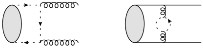
Figure 1: Examples of possible ghost contributions to the virtual corrections; due to the nature of the ghost coupling the diagram on the left hand side does not contribute in the soft limit. On the right hand side the ghost contribution for the gluon self energy is depicted, which needs to be included since it has the same momentum scaling as the three gluon vertex when all attached lines become soft.

We do however point out that when one wants to include collinear singular contributions a physical gauge is more advantageous. In this case we further face poles stemming from the propagator term involving the gauge vector $n$; in order to obtain the full $n$ (in)dependence it is vital to also consider the linear propagator terms introduced in the gluon propagator. If we limit our consideration to the light-cone gauge we can use the prescription Leibbrandt:Book

$$\frac{1}{n\cdot k}\to\frac{1}{n\cdot k+i0\ n^{*}\cdot k}\ ,$$ (31)

where $n^{*}=(n^{0},-\vec{n})$ for $n=(n^{0},\vec{n})$. This denominator implementing the Mandelstam/Leibbrandt prescription has a pole in the upper half-plane, if the spatial part of the loop momentum is anti-parallel to $\vec{n}$, and in the lower half-plane otherwise. The cutting rule is to assign a cut contribution $2\pi i\delta(n\cdot k)\theta(\vec{n}\cdot\vec{k})$ to such a gauge denominator, and accordingly we can build derivatives for higher powers.

4.2 Application to Two-Loop Integrals

The application of the Feynman tree theorem in the two-loop case is not unique as compared to the one-loop case. However, we can apply it to one of the one-loop sub-integrals, and then find a shift of the loop momenta such that the second loop momentum after the transformation is not affected by constraints of cuts from the previous application. If this is not possible, we terminate the algorithm. In this way we maximise the number of contributions of the two-loop integral which can directly be cast into a form of a double-emission phase space-type integral. After having cut in a first loop integration $k$ we determine, for each term in the sum over cuts, if we can shift the loop momenta $k,q\to k^{\prime},q^{\prime}$ in such a way that one loop integration, say $q^{\prime}$, only involves propagators and that no $\delta$ or $\theta$-function involves $q^{\prime}$. Then the $q^{\prime}$ integration can again be treated with the Feynman tree theorem. If this is not possible to perform such a momentum shift and both loop momenta are constrained by the $\delta$-functions already after the first application, or if the transformation $k,q\to k^{\prime},q^{\prime}$ would enforce a negative-energy $\theta$-function which has originated from the previous cut, the procedure terminates. The algorithm we outline here has been automated and we have used it to process all integrals required to calculate the two-loop soft integrals. We also exemplify the procedure in Fig. 2, which shows a detailed workflow for one of the topologies we have considered.

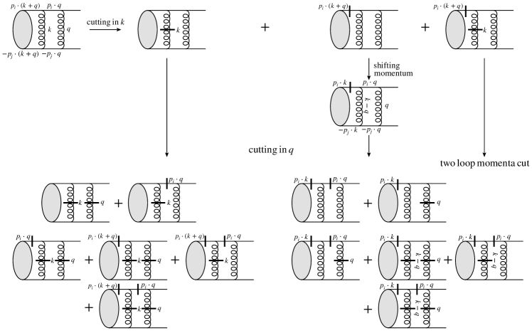
Figure 2: Illustration of the workflow when applying the Feynman tree theorem at the two-loop level. The short black lines symbolise cuts of the corresponding propagators.

Starting from the results for the two-loop integrals we then can choose an explicit parametrisation of the loop momentum in order to make contact with the phase space integrals over the real emission, and the resolution scale of the observable. At this stage, however, we only quote the (non-vanishing) cut contributions, including those which give rise to imaginary parts and will address a more concrete parametrisation tailored for specific observables in a future work. All of the relevant integrals in the two-loop, soft gluon case, are listed in Appendix C. The loop integrals which correspond to the $\Omega^{(2)}$-coefficients involving two hard lines are given by

$$\Omega^{(2)}_{ij}=-(p_{i}\cdot p_{j})(p_{i}\cdot p_{j})\,I^{(ij)}_{1}\ ,$$

$$\tilde{\Omega}^{(2)}_{ij}=-(p_{i}\cdot p_{j})(p_{i}\cdot p_{j})\,I^{(ij)}_{2}\ ,$$

$$\Omega^{(2)}_{ij,\mathrm{vertex-corr.}}=C_{A}\,(p_{i}\cdot p_{j})\left[2I^{(ij)}_{3}-I^{(ij)}_{4}\right]\ ,$$ (32)

$$\Omega^{(2)}_{ij,\mathrm{self-en.|gluon+ghost}}=2C_{A}\left[(4-2d)\,I^{(ij)}_{5}-2(p_{i}\cdot p_{j})\,I^{(ij)}_{3}-(p_{i}\cdot p_{j})\,I^{(ij)}_{6}\right]$$

$$\Omega^{(2)}_{ij,\mathrm{self-en.|fermion}}=4n_{f}\left[2I^{(ij)}_{5}-\frac{1}{2}(p_{i}\cdot p_{j})I^{(ij)}_{3}-(p_{i}\cdot p_{j})I^{(ij)}_{6}\right]\ ,$$

and involving three hard lines we find

$$\Omega^{(2)}_{ijl}=-(p_{i}\cdot p_{l})(p_{i}\cdot p_{j})\,I^{(ijl)}_{1}\ ,$$ (33)

$$\hat{\Omega}^{(2)}_{ijl}=2\left[(p_{j}\cdot p_{l})\,I^{(ijl)}_{2}-(p_{i}\cdot p_{j})\,I^{(ijl)}_{3}-(p_{i}\cdot p_{l})\,I^{(ijl)}_{4}\right]\ .$$

4.3 Application to Higher Propagator Powers

In the two-loop case we will also need to consider propagators at higher powers, in particular when a self-energy correction is inserted on an exchanged gluon. In order to find an analogous rule for treating propagators of higher powers, we consider the derivative of equation (29) with respect to the momentum $q^{\mu}$

$$\frac{q^{\mu}-i0T^{\mu}(T\cdot q)}{[q^{2}-i0(T\cdot q)^{2}]^{2}}-\frac{q^{\mu}+i0T^{\mu}(T\cdot q)}{[q^{2}+i0(T\cdot q)^{2}]^{2}}=-i\pi\frac{\partial}{\partial q^{\mu}}\delta(q^{2})\ .$$ (34)

The derivative of the $\delta$-function with respect to a momentum component can be left as a formal object until we can simplify this later by means of integration by parts. An alternative which we consider is to eliminate the $T$-dependent term in the numerator, contract with some vector $S^{\mu}$, which has the property $S\cdot T=0$, i.e. $S^{\mu}$ is space-like ($S^{2}<0$) to obtain

$$\begin{split}\frac{1}{[q^{2}-i0(T\cdot q)^{2}]^{2}}-\frac{1}{[q^{2}+i0(T\cdot q)^{2}]^{2}}&=-i\pi\frac{S_{\mu}}{S\cdot q}\frac{\partial}{\partial q^{\mu}}\delta(q^{2})\\ &=-2i\pi\delta^{\prime}(q^{2})\ ,\end{split}$$ (35)

where we define $\delta^{\prime}(q^{2})\equiv\frac{\partial}{\partial q^{2}}\delta(q^{2})$. This identity can then be supplemented by placing the double pole again in the upper half plane and we effectively use

$$\frac{1}{[q^{2}-i0(T\cdot q)|T\cdot q|]^{2}}-\frac{1}{[q^{2}+i0(T\cdot q)^{2}]^{2}}=-2i\pi\theta(T\cdot q)\delta^{\prime}(q^{2})\ .$$ (36)

Clearly this procedure can continue to even higher powers of propagators. In our case we require to apply Eq. (36) when considering a self-energy insertion on an exchanged gluon line. We note that, if we have not expressed the self energy in its integrated form but do want to apply our cutting procedure, then we will face $\delta^{\prime}$-distributions possibly in both loop integrations. We can ultimately only resolve these constraints using integration by parts once we have expressed the loop momenta in a certain parametrisation. An example of this procedure is to write

$$q^{\mu}=q_{+}\overline{n}^{\mu}+\frac{q^{2}-q_{\perp}^{2}}{2q_{+}(n\cdot\overline{n})}n^{\mu}+q_{\perp}^{\mu}\ ,$$ (37)

as this leads to the following expression for the derivative with respect to $q^{2}$

$$\frac{\partial q^{\mu}}{\partial q^{2}}=\frac{n^{\mu}}{2q_{+}(n\cdot\overline{n})}=\frac{n^{\mu}}{2(n\cdot q)}\ ,$$ (38)

with $q_{+}=\frac{n\cdot q}{n\cdot\overline{n}}$. No reference then needs to be made to the additional vectors $T^{\mu}$ and $S^{\mu}$ which we have been resorting to in setting up the derivative rule. In App. B we give expressions for the relevant integrals using this procedure.

4.4 One-loop, one-emission contributions

The integrands of the one-loop, one-emission diagrams have been treated with the modified Feynman tree theorem for Eikonal propagators. To ensure the applicability of the FTT we checked for each of the diagrams that the degrees of the polynomial in the loop-momentum of the propagators is bigger or equal to the polynomial of the numerator structure plus two. For the diagram involving the triple gluon vertex a tensor reduction can be performed prior to the application of the FTT. The cut-contributions which are obtained through this procedure for the one-loop, one-emission diagrams are listed in Appendix C.1. The coefficients $\Omega^{(1,1)}$ for two hard lines are given by

$$\Omega^{(1,1)}_{ij}=(-i)\frac{(p_{i}\cdot p_{j})}{p_{i}\cdot q}(p_{i}\cdot\varepsilon^{*}(q))\,I^{(ij)}_{7}\ ,$$

$$\tilde{\Omega}^{(1,1)}_{ij}=(-i)(p_{i}\cdot p_{j})(p_{i}\cdot\varepsilon^{*}(q))\,I^{(ij)}_{8}\ ,$$ (39)

$$\overline{\Omega}^{(1,1)}_{ij}=i\Bigg{\{}(p_{j}\cdot q)(p_{i}\cdot\varepsilon^{*}(q))\,I^{(ij)}_{9}-\frac{p_{i}\cdot q}{p_{j}\cdot q}(p_{j}\cdot\varepsilon^{*}(q))\,I^{(ij)}_{10}$$

$$\hskip 28.45274pt-\frac{p_{i}\cdot p_{j}}{2}\left[\frac{(p_{i}\cdot\varepsilon^{*}(q))}{p_{i}\cdot q}+\frac{(p_{j}\cdot\varepsilon^{*}(q))}{p_{j}\cdot q}\right]I^{(ij)}_{7}\Bigg{\}}\ ,$$

$$\Omega^{(1,1)}_{ij,\mathrm{vertex-corr.}}=C_{A}(p_{i}\cdot\varepsilon^{*}(q))\left[I^{(ij)}_{10}-\frac{2}{p_{i}\cdot q}I_{0}^{(ij)}\right]\ ,$$

where the loop integral described by $I^{(ij)}_{0}$ is scale-less and if the FTT is used one finds that it vanishes exactly for $p_{i}^{0}>0$ and on-shell external momenta. For the one-loop/one-emission contribution with three hard lines one gets the one-loop integral $\Omega^{(1)}_{il}$ (cf. Eq. (5))

$$\Omega^{(1,1)}_{ijl}=\frac{p_{i}\cdot p_{l}}{p_{j}\cdot q}(p_{j}\cdot\varepsilon^{*}(q))\,\Omega^{(1)}_{il}\ .$$ (40)

5 Conclusion and Outlook

In this paper we have been providing the basic ingredients to formulate soft gluon evolution at the next-to-leading order, using the colour flow basis, as well as the Feynman tree theorem, to express the relevant one-loop, one-emission and two-loop diagrams.

This will allow to perform the resummation of non-global observables at the next-to-leading logarithmic order, and provides crucial insight to the design of amplitude evolution algorithms and parton showers beyond the currently adopted approximations. In particular we have taken an entirely new approach towards virtual corrections, being able to cast them into a form in which we can make the cancellation of infrared divergencies explicit and determine the imaginary parts of the loop integrals in a way that we control the kinematic regions from which they originate. Results on this, assuming certain orderings, will be published elsewhere, while we have here presented the virtual corrections in a generic manner using a new method of applying the FTT to the two-loop case and to Eikonal propagators. All of our results are carried out in dimensional regularisation such that upon performing the actual integrals one could recover the poles in an expansion in $\epsilon\to 0$.

The analysis of the colour structure allows us to adopt a perturbative treatment of the amplitude evolution operators, or to explore more sophisticated Monte Carlo methods in colour space. Our analysis definitely highlights that a dipole-type picture is not anymore sufficient provided one concentrates not only on the strict leading colour approximation, but requires to include all colour diagonal contributions, an approximation which has turned out to be crucial within the leading-order context already, and certainly if one attempts to include collinear physics which probes such effects effectively as the difference between $C_{A}/2$ and $C_{F}$.

Appendix A Details on colour structures

In this appendix we quote the main results on the decomposition of the colour structures in the one-loop, one-emission as well as two loop cases, translating the colour structures into the colour flow basis and quoting the final result in terms of swaps and colour flows added after the emission. We quote those per diagram, as we have extracted them to separate the colour structures from the kinematic dependence.

A.1 One-loop, one-emission colour structures

• Gluon emission after the exchange:

$$\begin{split}[\tau|\mathbb{T}_{i}(\mathbb{T}_{i}\cdot\mathbb{T}_{j})|\sigma\rangle&=N^{2}\delta_{\sigma\tau\backslash n}\\ &\left[\frac{1}{N^{2}}(\lambda_{i}-\bar{\lambda}_{i})\left(\lambda_{i}\bar{\lambda}_{j}\delta_{c_{i}\sigma^{-1}(\overline{c}_{j})}\delta_{c_{n}\tau^{-1}(\overline{c}_{n})}+\bar{\lambda}_{i}\lambda_{j}\delta_{c_{j}\sigma^{-1}(\overline{c}_{i})}\delta_{c_{n}\tau^{-1}(\overline{c}_{n})}\right)\right.\\ &\left.+\frac{1}{N^{4}}(\lambda_{i}-\bar{\lambda}_{i})^{2}(\lambda_{j}-\bar{\lambda}_{j})\delta_{c_{n}\tau^{-1}(\overline{c}_{n})}\right]\\ &+\sum_{(a,b)}\delta_{\sigma\tau_{(a,b)}\backslash n}\\ &\bigg{[}N\left(\bar{\lambda}_{i}^{2}\lambda_{j}\delta_{c_{j}\sigma^{-1}(\overline{c}_{i})}\delta_{(a,b)(c_{j},c_{n})}-\lambda_{i}^{2}\bar{\lambda}_{j}\delta_{c_{i}\sigma^{-1}(\overline{c}_{j})}\delta_{(a,b)(c_{i},c_{n})}\right.\\ &\left.+\lambda_{i}\bar{\lambda}_{i}\lambda_{j}\delta_{c_{i}\sigma^{-1}(\overline{c}_{j})}\delta_{(a,b)(\sigma^{-1}(\overline{c}_{i}),c_{n})}-\lambda_{i}\bar{\lambda}_{i}\lambda_{j}\delta_{c_{j}\sigma^{-1}(\overline{c}_{i})}\delta_{(a,b)(c_{i},c_{n})}\right)\\ &+\frac{1}{N}\delta_{c_{n}\tau^{-1}(\overline{c}_{n})}(\lambda_{i}-\bar{\lambda}_{i})\left(\lambda_{i}\bar{\lambda}_{j}\delta_{(a,b)(c_{i},\sigma^{-1}(\overline{c}_{j}))}+\bar{\lambda}_{i}\lambda_{j}\delta_{(a,b)(c_{j},\sigma^{-1}(\overline{c}_{i}))}\right.\\ &\left.-\lambda_{i}\lambda_{j}\delta_{(a,b)(c_{i},c_{j})}-\bar{\lambda}_{i}\bar{\lambda}_{j}\delta_{(a,b)(\sigma^{-1}(\overline{c}_{j}),\sigma^{-1}(\overline{c}_{i}))}\right)\\ &-\frac{1}{N}(\lambda_{i}-\bar{\lambda}_{i})(\lambda_{j}-\bar{\lambda}_{j})\left(\lambda_{i}\delta_{(a,b)(c_{i},c_{n})}-\bar{\lambda}_{i}\delta_{(a,b)(\sigma^{-1}(\overline{c}_{i}),c_{n})}\right)\bigg{]}\\ &+\sum_{(a,b)}\sum_{(b,c)}\delta_{\sigma\tau_{(a,b)(b,c)}\backslash n}\\ &\left[\lambda_{i}^{2}\lambda_{j}\delta_{(a,b)(c_{n},c_{i})}\delta_{(b,c)(c_{i},c_{j})}+\bar{\lambda}_{i}^{2}\lambda_{j}\delta_{(a,b)(c_{n},c_{j})}\delta_{(b,c)(c_{j},\sigma^{-1}(\overline{c}_{i}))}\right.\\ &\left.-\lambda_{i}^{2}\bar{\lambda}_{j}\delta_{(a,b)(c_{n},c_{i})}\delta_{(b,c)(c_{i},\sigma^{-1}(\overline{c}_{j}))}-\bar{\lambda}_{i}^{2}\bar{\lambda}_{j}\delta_{(a,b)(c_{n},\sigma^{-1}(\overline{c}_{j}))}\delta_{(b,c)(\sigma^{-1}(\overline{c}_{j}),\sigma^{-1}(\overline{c}_{i}))}\right]\\ &+\sum_{(a,b)}\sum_{(c,d)}\delta_{\sigma\tau_{(a,b)(c,d)}\backslash n}\lambda_{i}\bar{\lambda}_{i}\\ &\left[\delta_{(a,b)(\sigma^{-1}(\overline{c}_{i}),c_{n})}\left(\bar{\lambda}_{j}\delta_{(c,d)(c_{i},\sigma^{-1}(\overline{c}_{j}))}-\lambda_{j}\delta_{(c,d)(c_{i},c_{j})}\right)\right.\\ &\left.+\delta_{(a,b)(c_{i},c_{n})}\left(\bar{\lambda}_{j}\delta_{(c,d)(\sigma^{-1}(\overline{c}_{i}),\sigma^{-1}(\overline{c}_{j}))}-\lambda_{j}\delta_{(c,d)(c_{j},\sigma^{-1}(\overline{c}_{i}))}\right)\right]\end{split}$$ (41)

• Triple gluon vertex:

$$\begin{split}[\tau|\mathbb{T}_{g}\mathbb{T}_{i}\mathbb{T}_{j}|\sigma\rangle&=\sqrt{T_{R}}\left\{\delta_{\sigma\tau\backslash n}\delta_{c_{n}\tau^{-1}(\overline{c}_{n})}\left[-\lambda_{i}\bar{\lambda}_{j}\delta_{c_{i}\sigma^{-1}(\overline{c}_{j})}+\bar{\lambda}_{i}\lambda_{j}\delta_{c_{j}\sigma^{-1}(\overline{c}_{i})}\right]\right.\\ &\left.+N\sum_{(a,b)}\delta_{\sigma\tau_{(a,b)}\backslash n}\left[\lambda_{i}\bar{\lambda}_{j}\delta_{c_{i}\sigma^{-1}(\overline{c}_{j})}\delta_{(a,b)(c_{i},c_{n})}-\bar{\lambda}_{i}\lambda_{j}\delta_{c_{j}\sigma^{-1}(\overline{c}_{i})}\delta_{(a,b)(c_{j},c_{n})}\right]\right.\\ &\left.+\sum_{(a,b)}\sum_{(b,c)}\delta_{\sigma\tau_{(a,b)(b,c)}\backslash n}\right.\\ &\left.\left[\lambda_{i}\bar{\lambda}_{j}\left(\delta_{(a,b)(c_{n},c_{i})}\delta_{(b,c)(c_{i},\sigma^{-1}(\overline{c}_{j}))}-\delta_{(a,b)(c_{n},\sigma^{-1}(\overline{c}_{j}))}\delta_{(b,c)(\sigma^{-1}(\overline{c}_{j}),c_{i})}\right)\right.\right.\\ &\left.\left.+\bar{\lambda}_{i}\lambda_{j}\left(\delta_{(a,b)(c_{n},\sigma^{-1}(\overline{c}_{i}))}\delta_{(b,c)(\sigma^{-1}(\overline{c}_{i}),c_{j})}-\delta_{(a,b)(c_{n},c_{j})}\delta_{(b,c)(c_{j},\sigma^{-1}(\overline{c}_{i}))}\right)\right.\right.\\ &\left.\left.+\lambda_{i}\lambda_{j}\left(\delta_{(a,b)(c_{n},c_{j})}\delta_{(b,c)(c_{j},c_{i})}-\delta_{(a,b)(c_{n},c_{i})}\delta_{(b,c)(c_{i},c_{j})}\right)\right.\right.\\ &\left.\left.+\bar{\lambda}_{i}\bar{\lambda}_{j}\left(\delta_{(a,b)(c_{n},\sigma^{-1}(\overline{c}_{j}))}\delta_{(b,c)(\sigma^{-1}(\overline{c}_{j}),\sigma^{-1}(\overline{c}_{i}))}\right.\right.\right.\\ &\left.\left.\left.-\delta_{(a,b)(c_{n},\sigma^{-1}(\overline{c}_{i}))}\delta_{(b,c)(\sigma^{-1}(\overline{c}_{i}),\sigma^{-1}(\overline{c}_{j}))}\right)\right]\right\}\end{split}$$ (42)

• Gluon emission and exchange involving three hard lines:

$$\begin{split}[\tau|(\mathbb{T}_{i}\cdot\mathbb{T}_{j})\mathbb{T}_{l}|\sigma\rangle=&N^{2}\delta_{\sigma\tau\backslash n}\delta_{c_{n}\tau^{-1}(\overline{c}_{n})}\left[\frac{1}{N^{4}}(\lambda_{i}-\bar{\lambda}_{i})(\lambda_{j}-\bar{\lambda}_{j})(\lambda_{l}-\bar{\lambda}_{l})\right.\\ &\left.+\frac{1}{N^{2}}\left(\bar{\lambda}_{i}\lambda_{j}(\lambda_{l}-\bar{\lambda}_{l})\delta_{c_{j}\sigma^{-1}(\overline{c}_{i})}+\lambda_{i}\bar{\lambda}_{j}(\lambda_{l}-\bar{\lambda}_{l})\delta_{c_{i}\sigma^{-1}(\overline{c}_{j})}\right)\right]\\ &+\sum_{(a,b)}\delta_{\sigma\tau_{(a,b)}\backslash n}\left[N\delta_{(a,b)(\sigma^{-1}(\overline{c}_{l}),c_{n})}\left(\lambda_{i}\bar{\lambda}_{j}\bar{\lambda}_{l}\delta_{c_{i}\sigma^{-1}(\overline{c}_{j})}+\bar{\lambda}_{i}\lambda_{j}\bar{\lambda}_{l}\delta_{c_{j}\sigma^{-1}(\overline{c}_{i}})\right)\right.\\ &\left.-N\delta_{(a,b)(c_{l},c_{n})}\left(\lambda_{i}\bar{\lambda}_{j}\lambda_{l}\delta_{c_{i}\sigma^{-1}(\overline{c}_{j})}+\bar{\lambda}_{i}\lambda_{j}\lambda_{l}\delta_{c_{j}\sigma^{-1}(\overline{c}_{i})}\right)\right.\\ &\left.+\frac{1}{N}(\lambda_{i}-\bar{\lambda}_{i})(\lambda_{j}-\bar{\lambda}_{j})\left(\bar{\lambda}_{l}\delta_{(a,b)(\sigma^{-1}(\overline{c}_{l}),c_{n})}-\lambda_{l}\delta_{(a,b)(c_{l},c_{n})}\right)\right.\\ &\left.+\frac{1}{N}\delta_{c_{n}\tau^{-1}(\overline{c}_{n})}(\lambda_{l}-\bar{\lambda}_{l})\left(\lambda_{i}\bar{\lambda}_{j}\delta_{(a,b)(c_{i},\sigma^{-1}(\overline{c}_{j}))}+\bar{\lambda}_{i}\lambda_{j}\delta_{(a,b)(\sigma^{-1}(\overline{c}_{i}),c_{j})}\right.\right.\\ &\left.\left.-\lambda_{i}\lambda_{j}\delta_{(a,b)(c_{i},c_{j})}-\bar{\lambda}_{i}\bar{\lambda}_{j}\delta_{(a,b)(\sigma^{-1}(\overline{c}_{i}),\sigma^{-1}(\overline{c}_{j}))}\right)\right]\\ &+\sum_{(a,b)}\sum_{(c,d)}\delta_{\sigma\tau_{(a,b)(c,d)}\backslash n}\\ &\left[-\lambda_{i}\bar{\lambda}_{l}\delta_{(a,b)(\sigma^{-1}(\overline{c}_{l}),c_{n})}\left(\lambda_{j}\delta_{(c,d)(c_{i},c_{j})}-\bar{\lambda}_{j}\delta_{(c,d)(c_{i},\sigma^{-1}(\overline{c}_{j}))}\right)\right.\\ &\left.+\bar{\lambda}_{i}\bar{\lambda}_{l}\delta_{(a,b)(\sigma^{-1}(\overline{c}_{l}),c_{n})}\left(\lambda_{j}\delta_{(c,d)(\sigma^{-1}(\overline{c}_{i}),c_{j}))}-\bar{\lambda}_{j}\delta_{(c,d)(\sigma^{-1}(\overline{c}_{i}),\sigma^{-1}(\overline{c}_{j}))}\right)\right.\\ &\left.+\lambda_{i}\lambda_{l}\delta_{(a,b)(c_{l},c_{n})}\left(\lambda_{j}\delta_{(c,d)(c_{i},c_{j})}-\bar{\lambda}_{j}\delta_{(c,d)(c_{i},\sigma^{-1}(\overline{c}_{j}))}\right)\right.\\ &\left.-\bar{\lambda}_{i}\lambda_{l}\delta_{(a,b)(c_{l},c_{n})}\left(\lambda_{j}\delta_{(c,d)(\sigma^{-1}(\overline{c}_{i}),c_{j})}-\bar{\lambda}_{j}\delta_{(c,d)(\sigma^{-1}(\overline{c}_{i}),\sigma^{-1}(\overline{c}_{j}))}\right)\right]\end{split}$$ (43)

• Gluon emission prior to exchange:

$$\begin{split}[\tau|(\mathbb{T}_{i}\cdot\mathbb{T}_{j})\mathbb{T}_{i}|\sigma\rangle&=N^{2}\delta_{\sigma\tau\backslash n}\delta_{c_{n}\tau^{-1}(\overline{c}_{n})}\left[\frac{1}{N^{2}}\left(\lambda_{i}\bar{\lambda}_{i}\lambda_{j}\delta_{c_{j}\sigma^{-1}(\overline{c}_{i})}-\lambda_{i}\bar{\lambda}_{i}\bar{\lambda}_{j}\delta_{c_{i}\sigma^{-1}(\overline{c}_{j})}\right)\right.\\ &\left.+\frac{1}{N^{4}}(\lambda_{i}-\bar{\lambda}_{i})^{2}(\lambda_{j}-\bar{\lambda}_{j})\right]\\ &+\sum_{(a,b)}\delta_{\sigma\tau_{(a,b)}\backslash n}\\ &\left[N\lambda_{i}\bar{\lambda}_{i}\left(\bar{\lambda}_{j}\delta_{c_{i}\sigma^{-1}(\overline{c}_{j})}\delta_{(a,b)(\sigma^{-1}(\overline{c}_{i}),c_{n})}-\lambda_{j}\delta_{c_{j}\sigma^{-1}(\overline{c}_{i})}\delta_{(a,b)(c_{i},c_{n})}\right)\right.\\ &\left.+\frac{1}{N}\delta_{c_{n}\tau^{-1}(\overline{c}_{n})}(\lambda_{i}-\bar{\lambda}_{i})\left(\bar{\lambda}_{j}\lambda_{i}\delta_{(a,b)(c_{i},\sigma^{-1}(\overline{c}_{j}))}+\bar{\lambda}_{i}\lambda_{j}\delta_{(a,b)(\sigma^{-1}(\overline{c}_{i}),c_{j})}\right.\right.\\ &\left.\left.-\lambda_{i}\lambda_{j}\delta_{(a,b)(c_{i},c_{j})}-\bar{\lambda}_{i}\bar{\lambda}_{j}\delta_{(a,b)(\sigma^{-1}(\overline{c}_{i}),\sigma^{-1}(\overline{c}_{j}))}\right)\right.\\ &\left.-\frac{1}{N}\lambda_{i}(\lambda_{i}-\bar{\lambda}_{i})(\lambda_{j}-\bar{\lambda}_{j})\delta_{(a,b)(c_{i},c_{n})}\right.\\ &\left.+\frac{1}{N}\bar{\lambda}_{i}(\lambda_{i}-\bar{\lambda}_{i})(\lambda_{j}-\bar{\lambda}_{j})\delta_{(a,b)(\sigma^{-1}(\overline{c}_{i}),c_{n})}\right]\\ &+\sum_{(a,b)}\sum_{(b,c)}\delta_{\sigma\tau_{(a,b)(b,c)}\backslash n}\\ &\left[\lambda_{i}^{2}\lambda_{j}\delta_{(a,b)(c_{n},c_{j})}\delta_{(b,c)(c_{j},c_{i})}+\bar{\lambda}_{i}^{2}\lambda_{j}\delta_{(a,b)(c_{n},\sigma^{-1}(\overline{c}_{i}))}\delta_{(b,c)(\sigma^{-1}(\overline{c}_{i}),c_{j})}\right.\\ &\left.-\lambda_{i}^{2}\bar{\lambda}_{j}\delta_{(a,b)(c_{n},\sigma^{-1}(\overline{c}_{j}))}\delta_{(b,c)(\sigma^{-1}(\overline{c}_{j}),c_{i})}\right.\\ &\left.-\bar{\lambda}_{i}^{2}\bar{\lambda}_{j}\delta_{(a,b)(c_{n},\sigma^{-1}(\overline{c}_{i}))}\delta_{(b,c)(\sigma^{-1}(\overline{c}_{i}),\sigma^{-1}(\overline{c}_{j}))}\right.\\ &\left.-\lambda_{i}\bar{\lambda}_{i}\lambda_{j}\delta_{c_{j}\sigma^{-1}(\overline{c}_{i})}\delta_{(a,b)(c_{n},c_{i})}\delta_{(b,c)(c_{i},c_{j})}\right.\\ &\left.+\lambda_{i}\bar{\lambda}_{i}\bar{\lambda}_{j}\delta_{c_{i}\sigma^{-1}(\overline{c}_{j})}\delta_{(a,b)(c_{n},c_{i})}\delta_{(b,c)(c_{i},\sigma^{-1}(\overline{c}_{i}))}\right]\\ &+\sum_{(a,b)}\sum_{(c,d)}\delta_{\sigma\tau_{(a,b)(c,d)}\backslash n}\lambda_{i}\bar{\lambda}_{i}\\ &\left[\bar{\lambda}_{j}\left(\delta_{(a,b)(\sigma^{-1}(\overline{c}_{i}),c_{n})}\delta_{(c,d)(c_{i},\sigma^{-1}(\overline{c}_{j}))}-\delta_{(a,b)(c_{i},c_{n})}\delta_{(c,d)(\sigma^{-1}(\overline{c}_{i}),\sigma^{-1}(\overline{c}_{j}))}\right)\right.\\ &\left.-\lambda_{j}\left(\delta_{(a,b)(\sigma^{-1}(\overline{c}_{i}),c_{n})}\delta_{(c,d)(c_{i},c_{j})}+\delta_{(a,b)(c_{i},c_{n})}\delta_{(c,d)(\sigma^{-1}(\overline{c}_{i}),c_{j})}\right)\right]\end{split}$$ (44)

A.2 Two-loop structures

• Double gluon exchange:

$$\begin{split}[\tau|(\mathbb{T}_{i}\cdot\mathbb{T}_{j})(\mathbb{T}_{i}\cdot\mathbb{T}_{j})|\sigma\rangle&=N^{2}\delta_{\sigma\tau}\\ &\bigg{[}\lambda_{i}^{2}\bar{\lambda}_{j}^{2}\delta_{c_{i}\sigma^{-1}(\overline{c}_{j})}+\bar{\lambda}_{i}^{2}\lambda_{j}^{2}\delta_{c_{j}\sigma^{-1}(\overline{c}_{i})}+2\lambda_{i}\bar{\lambda}_{i}\lambda_{j}\bar{\lambda}_{j}\delta_{c_{i}\sigma^{-1}(\overline{c}_{j})}\delta_{c_{j}\sigma^{-1}(\overline{c}_{i})}\\ &+\frac{2}{N^{2}}(\lambda_{i}-\bar{\lambda}_{i})(\lambda_{j}-\bar{\lambda}_{j})\left(\bar{\lambda}_{i}\lambda_{j}\delta_{c_{j}\sigma^{-1}(\overline{c}_{i})}+\lambda_{i}\bar{\lambda}_{j}\delta_{c_{i}\sigma^{-1}(\overline{c}_{j})}\right)\\ &+\frac{1}{N^{2}}\left(\lambda_{i}^{2}\lambda_{j}^{2}+\bar{\lambda}_{i}^{2}\bar{\lambda}_{j}^{2}\right)+\frac{1}{N^{4}}(\lambda_{i}-\bar{\lambda}_{i})^{2}(\lambda_{j}-\bar{\lambda}_{j})^{2}\bigg{]}\\ &+N\sum_{(a,b)}\delta_{\sigma\tau_{(a,b)}}\left[\lambda_{i}^{2}\bar{\lambda}_{j}^{2}\delta_{(a,b)(c_{i},\sigma^{-1}(\overline{c}_{j}))}+\bar{\lambda}_{i}^{2}\lambda_{j}^{2}\delta_{(a,b)(\sigma^{-1}(\overline{c}_{i}),c_{j})}\right.\\ &\left.+\frac{2}{N^{2}}(\lambda_{i}-\bar{\lambda}_{i})(\lambda_{j}-\bar{\lambda}_{j})\left(\lambda_{i}\bar{\lambda}_{j}\delta_{(a,b)(c_{i},\sigma^{-1}(\overline{c}_{j}))}+\bar{\lambda}_{i}\lambda_{j}\delta_{(a,b)(\sigma^{-1}(\overline{c}_{i}),c_{j})}\right.\right.\\ &\left.\left.-\lambda_{i}\lambda_{j}\delta_{(a,b)(c_{i},c_{j})}-\bar{\lambda}_{i}\bar{\lambda}_{j}\delta_{(a,b)(\sigma^{-1}(\overline{c}_{i}),\sigma^{-1}(\overline{c}_{j}))}\right)\right.\\ &\left.-\lambda_{i}\bar{\lambda}_{i}\left(\lambda_{j}^{2}\delta_{(a,b)(c_{i},c_{j})}\delta_{c_{j}\sigma^{-1}(\overline{c}_{i})}+\bar{\lambda}_{j}^{2}\delta_{(a,b)(c_{i},\sigma^{-1}(\overline{c}_{i}))}\delta_{c_{i}\sigma^{-1}(\overline{c}_{j})}\right)\right.\\ &\left.-\lambda_{j}\bar{\lambda}_{j}\left(\lambda_{i}^{2}\delta_{(a,b)(c_{i},c_{j})}\delta_{c_{i}\sigma^{-1}(\overline{c}_{j})}+\bar{\lambda}_{i}^{2}\delta_{(a,b)(c_{j},\sigma^{-1}(\overline{c}_{j}))}\delta_{c_{j}\sigma^{-1}(\overline{c}_{i})}\right)\right.\\ &\left.+2\lambda_{i}\bar{\lambda}_{i}\lambda_{j}\bar{\lambda}_{j}\left(\delta_{(a,b)(\sigma^{-1}(\overline{c}_{i}),c_{j})}\delta_{c_{i}\sigma^{-1}(\overline{c}_{j})}+\delta_{(a,b)(c_{i},\sigma^{-1}(\overline{c}_{j}))}\delta_{c_{j}\sigma^{-1}(\overline{c}_{i})}\right)\right]\\ &-\sum_{(a,b)}\sum_{(b,c)}\delta_{\sigma\tau_{(a,b)(b,c)}}\\ &\left[\lambda_{i}\bar{\lambda}_{i}\lambda_{j}^{2}\left(\delta_{(a,b)(c_{i},\sigma^{-1}(\overline{c}_{i}))}\delta_{(b,c)(\sigma^{-1}(\overline{c}_{i}),c_{j})}+\delta_{(a,b)(c_{i},c_{j})}\delta_{(b,c)(c_{j},\sigma^{-1}(\overline{c}_{i}))}\right)\right.\\ &\left.+\lambda_{j}\bar{\lambda}_{j}\lambda_{i}^{2}\left(\delta_{(a,b)(c_{i},\sigma^{-1}(\overline{c}_{j}))}\delta_{(b,c)(\sigma^{-1}(\overline{c}_{j}),c_{j}))}+\delta_{(a,b)(c_{i},c_{j})}\delta_{(b,c)(c_{j},\sigma^{-1}(\overline{c}_{j}))}\right)\right.\\ &\left.+\lambda_{i}\bar{\lambda}_{i}\bar{\lambda}_{j}^{2}\left(\delta_{(a,b)(c_{i},\sigma^{-1}(\overline{c}_{i}))}\delta_{(b,c)(\sigma^{-1}(\overline{c}_{i}),\sigma^{-1}(\overline{c}_{j}))}\right.\right.\\ &\left.\left.+\delta_{(a,b)(c_{i},\sigma^{-1}(\overline{c}_{j}))}\delta_{(b,c)(\sigma^{-1}(\overline{c}_{j}),\sigma^{-1}(\overline{c}_{i}))}\right)\right.\\ &\left.+\lambda_{j}\bar{\lambda}_{j}\bar{\lambda}_{i}^{2}\left(\delta_{(a,b)(\sigma^{-1}(\overline{c}_{i}),\sigma^{-1}(\overline{c}_{j}))}\delta_{(b,c)(\sigma^{-1}(\overline{c}_{j}),c_{j})}\right.\right.\\ &\left.\left.+\delta_{(a,b)(\sigma^{-1}(\overline{c}_{i}),c_{j})}\delta_{(b,c)(c_{j},\sigma^{-1}(\overline{c}_{j}))}\right)\right]\\ &+2\sum_{(a,b)}\sum_{(c,d)}\delta_{\sigma\tau_{(a,b)(c,d)}}\lambda_{i}\bar{\lambda}_{i}\lambda_{j}\bar{\lambda}_{j}\\ &\left[\delta_{(a,b)(c_{i},\sigma^{-1}(\overline{c}_{j}))}\delta_{(c,d)(\sigma^{-1}(\overline{c}_{i}),c_{j})}+\delta_{(a,b)(c_{i},c_{j})}\delta_{(c,d)(\sigma^{-1}(\overline{c}_{i}),\sigma^{-1}(\overline{c}_{j}))}\right]\end{split}$$ (45)

• Crossed double exchange:

$$\begin{split}[\tau|\mathbb{T}_{i}\mathbb{T}_{i}\mathbb{T}_{j}\mathbb{T}_{j}|\sigma\rangle&=N^{2}\delta_{\sigma\tau}\bigg{[}2\lambda_{i}\bar{\lambda}_{i}\lambda_{j}\bar{\lambda}_{j}\delta_{c_{i}\sigma^{-1}(\overline{c}_{j})}\delta_{c_{j}\sigma^{-1}(\overline{c}_{i})}\\ &+\frac{2}{N^{2}}(\lambda_{i}-\bar{\lambda}_{i})(\lambda_{j}-\bar{\lambda}_{j})(\lambda_{i}\bar{\lambda}_{j}\delta_{c_{i}\sigma^{-1}(\overline{c}_{j})}+\bar{\lambda}_{i}\lambda_{j}\delta_{c_{j}\sigma^{-1}(\overline{c}_{i})})\\ &+\frac{1}{N^{2}}\left(\lambda_{i}^{2}\bar{\lambda}_{j}^{2}+\bar{\lambda}_{i}^{2}\lambda_{j}^{2}\right)+\frac{1}{N^{4}}(\lambda_{i}-\bar{\lambda}_{i})^{2}(\lambda_{j}-\bar{\lambda}_{j})^{2}\bigg{]}\\ &+\sum_{(a,b)}\delta_{\sigma\tau_{(a,b)}}\left[N\lambda_{i}^{2}\lambda_{j}^{2}\delta_{(a,b)(c_{i},c_{j})}+N\bar{\lambda}_{i}^{2}\bar{\lambda}_{j}^{2}\delta_{(a,b)(\sigma^{-1}(\overline{c}_{i}),\sigma^{-1}(\overline{c}_{j}))}\right.\\ &\left.+2N\lambda_{i}\bar{\lambda}_{i}\lambda_{j}\bar{\lambda}_{j}\left(\delta_{c_{i}\sigma^{-1}(\overline{c}_{j})}\delta_{(a,b)(\sigma^{-1}(\overline{c}_{i}),c_{j})}+\delta_{c_{j}\sigma^{-1}(\overline{c}_{i})}\delta_{(a,b)(c_{i},\sigma^{-1}(\overline{c}_{j}))}\right)\right.\\ &\left.+\frac{2}{N}(\lambda_{i}-\bar{\lambda}_{i})(\lambda_{j}-\bar{\lambda}_{j})\left(\lambda_{i}\bar{\lambda}_{j}\delta_{(a,b)(c_{i},\sigma^{-1}(\overline{c}_{j}))}+\bar{\lambda}_{i}\lambda_{j}\delta_{(a,b)(c_{j},\sigma^{-1}(\overline{c}_{i}))}\right.\right.\\ &\left.\left.-\lambda_{i}\lambda_{j}\delta_{(a,b)(c_{i},c_{j})}-\bar{\lambda}_{i}\bar{\lambda}_{j}\delta_{(a,b)(\sigma^{-1}(\overline{c}_{i}),\sigma^{-1}(\overline{c}_{j}))}\right)\right]\\ &-\sum_{(a,b)}\sum_{(b,c)}\delta_{\sigma\tau_{(a,b)(b,c)}}\\ &\left[\lambda_{j}^{2}\lambda_{i}\bar{\lambda}_{i}\left(\delta_{(a,b)(c_{i},c_{j})}\delta_{(b,c)(c_{j},\sigma^{-1}(\overline{c}_{i})))}+\delta_{(a,b)(c_{i},\sigma^{-1}(\overline{c}_{i}))}\delta_{(b,c)(\sigma^{-1}(\overline{c}_{i}),c_{j})}\right)\right.\\ &\left.+\bar{\lambda}_{j}^{2}\lambda_{i}\bar{\lambda}_{i}\left(\delta_{(a,b)(c_{i},\sigma^{-1}(\overline{c}_{i}))}\delta_{(b,c)(\sigma^{-1}(\overline{c}_{i}),\sigma^{-1}(\overline{c}_{j}))}\right.\right.\\ &\left.\left.\hskip 45.52458pt+\delta_{(a,b)(c_{i},\sigma^{-1}(\overline{c}_{j}))}\delta_{(b,c)(\sigma^{-1}(\overline{c}_{j}),\sigma^{-1}(\overline{c}_{i}))}\right)\right.\\ &\left.+\bar{\lambda}_{i}^{2}\lambda_{j}\bar{\lambda}_{j}\left(\delta_{(a,b)(\sigma^{-1}(\overline{c}_{i}),c_{j})}\delta_{(b,c)(c_{j},\sigma^{-1}(\overline{c}_{j}))}\right.\right.\\ &\left.\left.\hskip 45.52458pt+\delta_{(a,b)(\sigma^{-1}(\overline{c}_{i}),\sigma^{-1}(\overline{c}_{j}))}\delta_{(b,c)(\sigma^{-1}(\overline{c}_{j}),c_{j})}\right)\right.\\ &\left.+\lambda_{i}^{2}\lambda_{j}\bar{\lambda}_{j}\left(\delta_{(a,b)(c_{i},\sigma^{-1}(\overline{c}_{j}))}\delta_{(b,c)(\sigma^{-1}(\overline{c}_{j}),c_{j})}+\delta_{(a,b)(c_{i},c_{j})}\delta_{(b,c)(c_{j},\sigma^{-1}(\overline{c}_{j}))}\right)\right]\\ &+2\sum_{(a,b)}\sum_{(c,d)}\delta_{\sigma\tau_{(a,b)(c,d)}}\lambda_{i}\bar{\lambda}_{i}\lambda_{j}\bar{\lambda}_{j}\left[\delta_{(a,b)(c_{i},\sigma^{-1}(\overline{c}_{j}))}\delta_{(c,d)(c_{j},\sigma^{-1}(\overline{c}_{i}))}\right.\\ &\left.+\delta_{(a,b)(c_{i},c_{j})}\delta_{(c,d)(\sigma^{-1}(\overline{c}_{i}),\sigma^{-1}(\overline{c}_{j}))}\right]\end{split}$$ (46)

• Triple gluon vertex connecting three hard lines:

$$\begin{split}[\tau|\mathbb{T}_{g}\mathbb{T}_{l}\mathbb{T}_{i}\mathbb{T}_{j}|\sigma\rangle&=\sqrt{T_{R}}N^{2}\delta_{\sigma\tau}\bigg{[}\frac{1}{N^{2}}\left((\lambda_{l}-\bar{\lambda}_{l})\left(\lambda_{i}\bar{\lambda}_{j}\delta_{c_{i}\sigma^{-1}(\overline{c}_{j})}-\lambda_{j}\bar{\lambda}_{i}\delta_{c_{j}\sigma^{-1}(\overline{c}_{i})}\right)\right.\\ &\left.+(\lambda_{j}-\bar{\lambda}_{j})\left(\bar{\lambda}_{i}\lambda_{l}\delta_{c_{l}\sigma^{-1}(\overline{c}_{i})}-\lambda_{i}\bar{\lambda}_{l}\delta_{c_{i}\sigma^{-1}(\overline{c}_{l})}\right)\right.\\ &\left.+(\lambda_{i}-\bar{\lambda}_{i})\left(\bar{\lambda}_{l}\lambda_{j}\delta_{c_{j}\sigma^{-1}(\overline{c}_{l})}-\bar{\lambda}_{j}\lambda_{l}\delta_{c_{l}\sigma^{-1}(\overline{c}_{j})}\right)\right)\bigg{]}\\ &+\sum_{(a,b)}\delta_{\sigma\tau_{(a,b)}}N\sqrt{T_{R}}\left[\lambda_{i}\bar{\lambda}_{j}\lambda_{l}\delta_{(a,b)(c_{i},c_{l})}\left(\delta_{c_{l}\sigma^{-1}(\overline{c}_{j})}-\delta_{c_{i}\sigma^{-1}(\overline{c}_{j})}\right)\right.\\ &\left.+\bar{\lambda}_{i}\lambda_{j}\lambda_{l}\delta_{(a,b)(c_{j},c_{l})}\left(\delta_{c_{j}\sigma^{-1}(\overline{c}_{i})}-\delta_{c_{l}\sigma^{-1}(\overline{c}_{i})}\right)\right.\\ &\left.+\lambda_{i}\lambda_{j}\bar{\lambda}_{l}\delta_{(a,b)(c_{i},c_{j})}\left(\delta_{c_{i}\sigma^{-1}(\overline{c}_{l})}-\delta_{c_{j}\sigma^{-1}(\overline{c}_{l})}\right)\right.\\ &\left.+\lambda_{i}\bar{\lambda}_{j}\bar{\lambda}_{l}\left(\delta_{(a,b)(c_{i},\sigma^{-1}(\overline{c}_{l}))}\delta_{c_{i}\sigma^{-1}(\overline{c}_{j})}-\delta_{(a,b)(c_{i},\sigma^{-1}(\overline{c}_{j}))}\delta_{c_{i}\sigma^{-1}(\overline{c}_{l})}\right)\right.\\ &\left.+\bar{\lambda}_{i}\lambda_{j}\bar{\lambda}_{l}\left(\delta_{(a,b)(\sigma^{-1}(\overline{c}_{i}),c_{j})}\delta_{c_{j}\sigma^{-1}(\overline{c}_{l})}-\delta_{(a,b)(c_{j},\sigma^{-1}(\overline{c}_{l}))}\delta_{c_{j}\sigma^{-1}(\overline{c}_{i})}\right)\right.\\ &\left.+\bar{\lambda}_{i}\bar{\lambda}_{j}\lambda_{l}\left(\delta_{(a,b)(\sigma^{-1}(\overline{c}_{j}),c_{l})}\delta_{c_{l}\sigma^{-1}(\overline{c}_{i})}-\delta_{(a,b)(\sigma^{-1}(\overline{c}_{i}),c_{l})}\delta_{c_{l}\sigma^{-1}(\overline{c}_{j})}\right)\right]\\ &+\sum_{(a,b)}\sum_{(b,c)}\delta_{\sigma\tau_{(a,b)(b,c)}}\sqrt{T_{R}}\left[\lambda_{i}\lambda_{j}\delta_{(a,b)(c_{i},c_{j})}\left(\lambda_{l}\delta_{(b,c)(c_{j},c_{l})}-\bar{\lambda}_{l}\delta_{(b,c)(c_{j},\sigma^{-1}(\overline{c}_{l}))}\right)\right.\\ &\left.-\lambda_{i}\lambda_{l}\delta_{(a,b)(c_{i},c_{l})}\left(\lambda_{j}\delta_{(b,c)(c_{l},c_{j})}-\bar{\lambda}_{j}\delta_{(b,c)(c_{l},\sigma^{-1}(\overline{c}_{j}))}\right)\right.\\ &\left.-\lambda_{i}\bar{\lambda}_{j}\delta_{(a,b)(c_{i},\sigma^{-1}(\overline{c}_{j}))}\left(\lambda_{l}\delta_{(b,c)(\sigma^{-1}(\overline{c}_{j}),c_{l})}-\bar{\lambda}_{l}\delta_{(b,c)(\sigma^{-1}(\overline{c}_{j}),\sigma^{-1}(\overline{c}_{l}))}\right)\right.\\ &\left.+\bar{\lambda}_{i}\lambda_{l}\delta_{(a,b)(\sigma^{-1}(\overline{c}_{i}),c_{l})}\left(\lambda_{j}\delta_{(b,c)(c_{l},c_{j})}-\bar{\lambda}_{j}\delta_{(b,c)(c_{l},\sigma^{-1}(\overline{c}_{j}))}\right)\right.\\ &\left.-\bar{\lambda}_{i}\lambda_{j}\delta_{(a,b)(\sigma^{-1}(\overline{c}_{i}),c_{j})}\left(\lambda_{l}\delta_{(b,c)(c_{j},c_{l})}-\bar{\lambda}_{l}\delta_{(b,c)(c_{j},\sigma^{-1}(\overline{c}_{l}))}\right)\right.\\ &\left.-\bar{\lambda}_{i}\bar{\lambda}_{l}\delta_{(a,b)(\sigma^{-1}(\overline{c}_{i}),\sigma^{-1}(\overline{c}_{l}))}\left(\lambda_{j}\delta_{(b,c)(\sigma^{-1}(\overline{c}_{l}),c_{j})}-\bar{\lambda}_{j}\delta_{(b,c)(\sigma^{-1}(\overline{c}_{l}),\sigma^{-1}(\overline{c}_{j}))}\right)\right.\\ &\left.+\lambda_{i}\bar{\lambda}_{l}\delta_{(a,b)(c_{i},\sigma^{-1}(\overline{c}_{l}))}\left(\lambda_{j}\delta_{(b,c)(\sigma^{-1}(\overline{c}_{l}),c_{j})}-\bar{\lambda}_{j}\delta_{(b,c)(\sigma^{-1}(\overline{c}_{l}),\sigma^{-1}(\overline{c}_{j}))}\right)\right.\\ &\left.+\bar{\lambda}_{i}\bar{\lambda}_{j}\delta_{(a,b)(\sigma^{-1}(\overline{c}_{i}),\sigma^{-1}(\overline{c}_{j}))}\left(\lambda_{l}\delta_{(b,c)(\sigma^{-1}(\overline{c}_{j}),c_{l})}-\bar{\lambda}_{l}\delta_{(b,c)(\sigma^{-1}(\overline{c}_{j}),\sigma^{-1}(\overline{c}_{l}))}\right)\right]\end{split}$$ (47)

• Double gluon exchange between three hard lines:

$$\begin{split}[\tau|(\mathbb{T}_{i}\cdot\mathbb{T}_{l})(\mathbb{T}_{i}\cdot\mathbb{T}_{j})|\sigma\rangle&=N^{2}\delta_{\sigma\tau}\\ &\bigg{[}-\lambda_{i}\bar{\lambda}_{i}\left(\lambda_{j}\bar{\lambda}_{l}\delta_{c_{i}\sigma^{-1}(\overline{c}_{l})}\delta_{c_{j}\sigma^{-1}(\overline{c}_{i})}+\bar{\lambda}_{j}\lambda_{l}\delta_{c_{i}\sigma^{-1}(\overline{c}_{j})}\delta_{c_{l}\sigma^{-1}(\overline{c}_{i})}\right)\\ &+\frac{1}{N^{2}}(\lambda_{i}-\bar{\lambda}_{i})(\lambda_{l}-\bar{\lambda}_{l})\left(\lambda_{i}\bar{\lambda}_{j}\delta_{c_{i}\sigma^{-1}(\overline{c}_{j})}+\bar{\lambda}_{i}\lambda_{j}\delta_{c_{j}\sigma^{-1}(\overline{c}_{i})}\right)\\ &-\frac{1}{N^{2}}\left(\lambda_{i}^{2}\bar{\lambda}_{j}\lambda_{l}\delta_{c_{l}\sigma^{-1}(\overline{c}_{j})}+\bar{\lambda}_{i}^{2}\lambda_{j}\bar{\lambda}_{l}\delta_{c_{j}\sigma^{-1}(\overline{c}_{l})}\right)\\ &+\frac{1}{N^{2}}\lambda_{i}\bar{\lambda}_{i}(\lambda_{j}-\bar{\lambda}_{j})\left(\bar{\lambda}_{l}\delta_{c_{i}\sigma^{-1}(\overline{c}_{l})}-\lambda_{l}\delta_{c_{l}\sigma^{-1}(\overline{c}_{i})}\right)\\ &+\frac{1}{N^{4}}(\lambda_{i}-\bar{\lambda}_{i})^{2}(\lambda_{j}-\bar{\lambda}_{j})(\lambda_{l}-\bar{\lambda}_{l})\bigg{]}\\ &+\sum_{(ab)}\delta_{\sigma\tau_{(a,b)}}\\ &\left\{N\lambda_{i}\bar{\lambda}_{i}\left[\lambda_{j}\delta_{c_{j}\sigma^{-1}(\overline{c}_{i})}\left(\lambda_{l}\delta_{(a,b)(c_{i},c_{l})}-\bar{\lambda}_{l}\delta_{(a,b)(c_{i},\sigma^{-1}(\overline{c}_{l}))}\right)\right.\right.\\ &\left.\left.+\lambda_{l}\delta_{c_{l}\sigma^{-1}(\overline{c}_{i})}\left(\lambda_{j}\delta_{(a,b)(c_{i},c_{j})}-\bar{\lambda}_{j}\delta_{(a,b)(c_{i},\sigma^{-1}(\overline{c}_{j}))}\right)\right.\right.\\ &\left.\left.-\bar{\lambda}_{l}\delta_{c_{i}\sigma^{-1}(\overline{c}_{l})}\left(\lambda_{j}\delta_{(a,b)(\sigma^{-1}(\overline{c}_{i}),c_{j})}-\bar{\lambda}_{j}\delta_{(a,b)(\sigma^{-1}(\overline{c}_{i}),\sigma^{-1}(\overline{c}_{j}))}\right)\right.\right.\\ &\left.\left.-\bar{\lambda}_{j}\delta_{c_{i}\sigma^{-1}(\overline{c}_{j})}\left(\lambda_{l}\delta_{(a,b)(\sigma^{-1}(\overline{c}_{i}),c_{l})}-\bar{\lambda}_{l}\delta_{(a,b)(\sigma^{-1}(\overline{c}_{i}),\sigma^{-1}(\overline{c}_{l}))}\right)\right]\right.\\ &\left.+N\left[-\lambda_{i}^{2}\bar{\lambda}_{j}\delta_{c_{i}\sigma^{-1}(\overline{c}_{j})}\left(\lambda_{l}\delta_{(a,b)(c_{i},c_{l})}-\bar{\lambda}_{l}\delta_{(a,b)(c_{i},\sigma^{-1}(\overline{c}_{l}))}\right)\right.\right.\\ &\left.\left.+\bar{\lambda}_{i}^{2}\lambda_{j}\delta_{c_{j}\sigma^{-1}(\overline{c}_{i})}\left(\lambda_{l}\delta_{(a,b)(c_{j},c_{l})}-\bar{\lambda}_{l}\delta_{(a,b)(c_{j},\sigma^{-1}(\overline{c}_{l}))}\right)\right.\right.\\ &\left.\left.-\bar{\lambda}_{i}^{2}\bar{\lambda}_{j}\lambda_{l}\delta_{c_{l}\sigma^{-1}(\overline{c}_{j})}\delta_{(a,b)(\sigma^{-1}(\overline{c}_{i}),c_{l})}-\lambda_{i}^{2}\lambda_{j}\bar{\lambda}_{l}\delta_{c_{j}\sigma^{-1}(\overline{c}_{i})}\delta_{(a,b)(c_{i},c_{j})}\right]\right.\\ &\left.+\frac{1}{N}(\lambda_{i}-\bar{\lambda}_{i})\Big{[}(\lambda_{j}-\bar{\lambda}_{j})\left(\lambda_{i}\bar{\lambda}_{l}\delta_{(a,b)(c_{i},\sigma^{-1}(\overline{c}_{l}))}-\lambda_{i}\lambda_{l}\delta_{(a,b)(c_{i},c_{l})}\right.\right.\\ &\left.\left.+\bar{\lambda}_{i}\lambda_{l}\delta_{(a,b)(\sigma^{-1}(\overline{c}_{i}),c_{l})}-\bar{\lambda}_{i}\bar{\lambda}_{l}\delta_{(a,b)(\sigma^{-1}(\overline{c}_{i}),\sigma^{-1}(\overline{c}_{l}))}\right)\right.\\ &\left.+(\lambda_{l}-\bar{\lambda}_{l})\left(\lambda_{i}\bar{\lambda}_{j}\delta_{(a,b)(c_{i},\sigma^{-1}(\overline{c}_{j}))}+\bar{\lambda}_{i}\lambda_{j}\delta_{(a,b)(\sigma^{-1}(\overline{c}_{i}),c_{j})}\right.\right.\\ &\left.\left.-\lambda_{i}\lambda_{j}\delta_{(a,b)(c_{i},c_{j})}-\bar{\lambda}_{i}\bar{\lambda}_{j}\delta_{(a,b)(\sigma^{-1}(\overline{c}_{i}),\sigma^{-1}(\overline{c}_{j}))}\right)\Big{]}\right\}\\ &+\sum_{(a,b)}\sum_{(b,c)}\delta_{\sigma\tau_{(a,b)(b,c)}}\\ &\left\{\lambda_{i}^{2}\lambda_{j}\delta_{(a,b)(c_{i},c_{j})}\left(\lambda_{l}\delta_{(b,c)(c_{j},c_{l})}-\bar{\lambda}_{l}\delta_{(b,c)(c_{j},\sigma^{-1}(\overline{c}_{l}))}\right)\right.\\ &\left.+\bar{\lambda}_{i}^{2}\lambda_{l}\delta_{(a,b)(\sigma^{-1}(\overline{c}_{i}),c_{l})}\left(\lambda_{j}\delta_{(b,c)(c_{l},c_{j})}-\bar{\lambda}_{j}\delta_{(b,c)(c_{l},\sigma^{-1}(\overline{c}_{j}))}\right)\right.\\ &\left.-\bar{\lambda}_{i}^{2}\bar{\lambda}_{l}\delta_{(a,b)(\sigma^{-1}(\overline{c}_{i}),\sigma^{-1}(\overline{c}_{l}))}\left(\lambda_{j}\delta_{(b,c)(\sigma^{-1}(\overline{c}_{l}),c_{j})}-\bar{\lambda}_{j}\delta_{(b,c)(\sigma^{-1}(\overline{c}_{l}),\sigma^{-1}(\overline{c}_{j}))}\right)\right.\\ &\left.-\lambda_{i}^{2}\bar{\lambda}_{j}\delta_{(a,b)(c_{i},\sigma^{-1}(\overline{c}_{j}))}\left(\lambda_{l}\delta_{(b,c)(\sigma^{-1}(\overline{c}_{j}),c_{l})}-\bar{\lambda}_{l}\delta_{(b,c)(\sigma^{-1}(\overline{c}_{j}),\sigma^{-1}(\overline{c}_{l}))}\right)\right\}\\ &+\sum_{(a,b)}\sum_{(c,d)}\delta_{\sigma\tau_{(a,b)(c,d)}}\lambda_{i}\bar{\lambda}_{i}\\ &\left[\lambda_{j}\delta_{(a,b)(c_{i},c_{j})}\left(\lambda_{l}\delta_{(c,d)(\sigma^{-1}(\overline{c}_{i}),c_{l})}-\bar{\lambda}_{l}\delta_{(c,d)(\sigma^{-1}(\overline{c}_{i}),\sigma^{-1}(\overline{c}_{l}))}\right)\right.\\ &\left.-\bar{\lambda}_{j}\delta_{(a,b)(c_{i},\sigma^{-1}(\overline{c}_{j}))}\left(\lambda_{l}\delta_{(c,d)(\sigma^{-1}(\overline{c}_{i}),c_{l})}-\bar{\lambda}_{l}\delta_{(c,d)(\sigma^{-1}(\overline{c}_{i}),\sigma^{-1}(\overline{c}_{l}))}\right)\right.\\ &\left.+\lambda_{l}\delta_{(a,b)(c_{i},c_{l})}\left(\lambda_{j}\delta_{(c,d)(\sigma^{-1}(\overline{c}_{i}),c_{j})}-\bar{\lambda}_{j}\delta_{(c,d)(\sigma^{-1}(\overline{c}_{i}),\sigma^{-1}(\overline{c}_{j}))}\right)\right.\\ &\left.-\bar{\lambda}_{l}\delta_{(a,b)(c_{i},\sigma^{-1}(\overline{c}_{l}))}\left(\lambda_{j}\delta_{(c,d)(\sigma^{-1}(\overline{c}_{i}),c_{j})}-\bar{\lambda}_{j}\delta_{(c,d)(\sigma^{-1}(\overline{c}_{i}),\sigma^{-1}(\overline{c}_{j}))}\right)\right]\end{split}$$ (48)

Appendix B Diagrams involving the gluon self energy

The gluon self energy diagrams at two-loop level can be expressed in the following form after reduction (neglecting terms which vanish due to colour conservation)

$$\begin{split}\begin{gathered}\vspace{-0.2cm}\includegraphics[width=62.59596pt]{2loop_gluonbub}\end{gathered}+\begin{gathered}\vspace{-0.2cm}\includegraphics[width=61.17325pt]{2loop_ghostbub}\end{gathered}=&\frac{\alpha_{s}^{2}}{2}\sum_{i,j}T_{R}(\mathbb{T}_{i}\cdot\mathbb{T}_{j})\,2C_{A}\\ &\left[(4-2d)I_{5}^{(ij)}-2(p_{i}\cdot p_{j})I_{3}^{(ij)}-(p_{i}\cdot p_{j})I_{6}^{(ij)}\right]\ ,\end{split}$$ (49)

and

$$\begin{split}\begin{gathered}\vspace{-0.2cm}\includegraphics[width=62.59596pt]{2loop_fermionbub}\end{gathered}=&\frac{\alpha_{s}^{2}}{2}\sum_{i,j}4T_{R}(\mathbb{T}_{i}\cdot\mathbb{T}_{j})\,n_{f}\left[2I_{5}^{(ij)}-\frac{1}{2}(p_{i}\cdot p_{j})I_{3}^{(ij)}-(p_{i}\cdot p_{j})I_{6}^{(ij)}\right]\ .\end{split}$$ (50)

Again, we have used unordered colour sums. This requires the inclusion of a factor of $1/2$ in order to avoid overcounting for the bubble diagrams.
The loop integrals pertaining to the diagrams above are given by

$$\begin{split}&I^{(ij)}_{5}=\mu^{4\epsilon}\int_{k,q}\frac{(p_{i}\cdot k)(p_{j}\cdot k)}{[p_{i}\cdot q+i0][-p_{j}\cdot q+i0][k^{2}+i0][(q-k)^{2}+i0][q^{2}+i0]^{2}}\ ,\\ &I^{(ij)}_{6}=\mu^{4\epsilon}\int_{k,q}\frac{1}{[p_{i}\cdot q+i0][-p_{j}\cdot q+i0][k^{2}+i0][q^{2}+i0]^{2}}\ ,\\ &I^{(ij)}_{3}=\mu^{4\epsilon}\int_{k,q}\frac{1}{[p_{i}\cdot q+i0][-p_{j}\cdot q+i0][k^{2}+i0][(q-k)^{2}+i0][q^{2}+i0]}\ ,\end{split}$$ (51)

where we have used the short-hand notation $\int_{k,q}\equiv\int\frac{\mathrm{d\bar{}\hskip 0.70004pt}^{d}k}{i\pi^{d/2}}\int\frac{\mathrm{d\bar{}\hskip 0.70004pt}^{d}q}{i\pi^{d/2}}$. Furthermore note that according to our definition the $i0$-prescription of an Eikonal propagator with momentum $p_{i}$ is given by $i0(T\cdot p_{i})^{2}$ and for the soft gluon propagator of momentum $q$ we have $i0(T\cdot q)^{2}$. To avoid clutter we do not explicitly write these factors for the $i0$-prescription in the following. However, they can be easily reinstated with the rule above.
The contribution $I^{(ij)}_{3}$ does not contain a propagator to second power anymore. Due to its propagator structure this contribution is treated in App. C.2, Eq. (69). For the contributions with higher order propagators we find

$$\begin{split}I^{(ij)}_{5}=\mu^{4\epsilon}\int_{k,q}(p_{i}\cdot k)(p_{j}\cdot k)&\left\{-\frac{(2\pi i)^{2}\tilde{\delta}(q)\tilde{\delta}(k)}{[p_{i}\cdot(k+q)+i0][-p_{j}\cdot(k+q)+i0][(k+q)^{2}+i0]^{2}}\right.\\ &\left.+\frac{2(2\pi i)^{2}\tilde{\delta}(k)\delta(p_{i}\cdot q)}{[-p_{j}\cdot q+i0][(q-k)^{2}+i0][q^{2}+i0]^{2}}\right.\\ &\left.+\frac{2(2\pi i)^{2}(-\delta^{\prime}(q^{2})\theta(q^{0}))\tilde{\delta}(k)}{[p_{i}\cdot q+i0][-p_{j}\cdot q+i0][(q-k)^{2}+i0]}\right.\\ &\left.+\frac{2(2\pi i)^{3}\tilde{\delta}(k)\tilde{\delta}(q-k)\delta(p_{i}\cdot q)}{[-p_{j}\cdot q+i0][q^{2}+i0]^{2}}\right.\\ &\left.+\frac{2(2\pi i)^{3}(-\delta^{\prime}(q^{2})\theta(q^{0}))\tilde{\delta}(k)\delta(p_{i}\cdot q)}{[-p_{j}\cdot q+i0][(q-k)^{2}+i0]}\right.\\ &\left.+\frac{2(2\pi i)^{3}(-\delta^{\prime}(q^{2})\theta(q^{0}))\tilde{\delta}(k)\tilde{\delta}(q-k)}{[p_{i}\cdot q+i0][-p_{j}\cdot q+i0]}\right.\\ &\left.+\frac{2(2\pi i)^{4}(-\delta^{\prime}(q^{2})\theta(q^{0}))\tilde{\delta}(k)\tilde{\delta}(q-k)\delta(p_{i}\cdot q)}{[-p_{j}\cdot q+i0]}\right\}\ ,\end{split}$$ (52)

$$\begin{split}I^{(ij)}_{6}=\mu^{4\epsilon}\int_{k,q}&\left\{\frac{(2\pi i)^{2}\tilde{\delta}(k)\delta(p_{i}\cdot q)}{[-p_{j}\cdot q+i0][q^{2}+i0]^{2}}+\frac{(2\pi i)^{2}(-\delta^{\prime}(q^{2})\theta(q^{0}))\tilde{\delta}(k)}{[p_{i}\cdot q+i0][-p_{j}\cdot q+i0]}\right.\\ &\left.+\frac{(2\pi i)^{3}(-\delta^{\prime}(q^{2})\theta(q^{0}))\tilde{\delta}(k)\delta(p_{i}\cdot q)}{[-p_{j}\cdot q+i0]}\right\}\ .\end{split}$$ (53)

Appendix C List of integrals

C.1 One loop and one emission

Performing a Passarino-Veltman reduction one obtains the following contributions for the diagrams at one-loop, one-emission order

$$\begin{gathered}\hskip 5.69046pt\vspace{0.1cm}\includegraphics[width=62.59596pt]{singleline11_1}\end{gathered}=\alpha_{s}\,g\sum_{i,j}T_{R}\mathbb{T}_{i}^{a}C_{A}(p_{i}\cdot\varepsilon^{*}(q))\left[I_{10}^{(ij)}-\frac{2}{p_{i}\cdot q}I_{0}^{(ij)}\right]\ ,$$ (54)

$$\begin{gathered}\vspace{-0.2cm}\includegraphics[width=62.59596pt]{doubleline11_1}\end{gathered}=\alpha_{s}\,g\sum_{i,j}\mathbb{T}_{i}^{a}(\mathbb{T}_{i}\cdot\mathbb{T}_{j})(-i)\frac{p_{i}\cdot p_{j}}{p_{i}\cdot q}(p_{i}\cdot\varepsilon^{*}(q))I_{7}^{(ij)}\ ,$$ (55)

$$\begin{gathered}\hskip 2.84544pt\vspace{-0.2cm}\includegraphics[width=62.59596pt]{doubleline11_2}\end{gathered}=\alpha_{s}\,g\sum_{i,j}(\mathbb{T}_{i}\cdot\mathbb{T}_{j})\mathbb{T}_{i}^{a}(-i)(p_{i}\cdot p_{j})(p_{i}\cdot\varepsilon^{*}(q))I_{8}^{(ij)}\ ,$$ (56)

$$\begin{split}\begin{gathered}\vspace{-0.2cm}\includegraphics[width=62.59596pt]{doubleline11_3}\end{gathered}=&-\frac{\alpha_{s}\,g}{2}\sum_{i,j}f^{abc}\mathbb{T}_{i}^{b}\mathbb{T}_{j}^{c}\Bigg{\{}(p_{j}\cdot q)(p_{i}\cdot\varepsilon^{*}(q))I_{9}^{(ij)}\\ &-\frac{p_{i}\cdot q}{p_{j}\cdot q}(p_{j}\cdot\varepsilon^{*}(q))I_{10}^{(ij)}-\frac{p_{i}\cdot p_{j}}{2}\left[\frac{p_{i}\cdot\varepsilon^{*}(q)}{p_{i}\cdot q}+\frac{p_{j}\cdot\varepsilon^{*}(q)}{p_{j}\cdot q}\right]I_{7}^{(ij)}\Bigg{\}}\ ,\end{split}$$ (57)

The integrals in the equations above are given by

$$I^{(ij)}_{7}=\mu^{2\epsilon}\int_{k}\frac{1}{[p_{i}\cdot(k+q)+i0][-p_{j}\cdot k+i0][k^{2}+i0]},$$ (58)

$$I^{(ij)}_{8}=\mu^{2\epsilon}\int_{k}\frac{1}{[p_{i}\cdot(k+q)+i0][p_{i}\cdot k+i0][-p_{j}\cdot k+i0][k^{2}+i0]},$$

$$I^{(ij)}_{9}=\mu^{2\epsilon}\int_{k}\frac{1}{[p_{i}\cdot(k+q)+i0][-p_{j}\cdot k+i0][k^{2}+i0][(k+q)^{2}+i0]},$$

$$I^{(ij)}_{10}=\mu^{2\epsilon}\int_{k}\frac{1}{[-p_{i}\cdot k+i0][k^{2}+i0][(k+q)^{2}+i0]},$$

$$I^{(ij)}_{0}=\mu^{2\epsilon}\int_{k}\frac{1}{[(k+q)^{2}+i0][k^{2}+i0]}\ .$$

Using the Feynman tree theorem and filtering out contributions which give zero, such as $\tilde{\delta}(k)\delta(p_{i}\cdot(k+q))$ and $\tilde{\delta}(k)\delta(p_{i}\cdot(k+q))\delta(k\cdot q)$ - for $q$ being on-shell the conditions for $E_{k}$ lead to a contradiction - results in

$$\begin{split}I^{(ij)}_{7}=-\mu^{2\epsilon}\int_{k}&\left\{\frac{(2\pi i)\tilde{\delta}(k)}{[p_{i}\cdot(k+q)+i0][-p_{j}\cdot k+i0]}+\frac{(2\pi i)\delta(p_{i}\cdot k)}{[(k-q)^{2}+i0][p_{j}\cdot(q-k)+i0]}\right.\\ &\left.+\frac{(2\pi i)^{2}\tilde{\delta}(k)\delta(p_{i}\cdot(k+q))}{[-p_{j}\cdot k+i0]}\right\}\ ,\end{split}$$ (59)

$$\begin{split}I^{(ij)}_{8}=-\mu^{2\epsilon}\int_{k}&\left\{\frac{(2\pi i)\tilde{\delta}(k)}{[p_{i}\cdot(k+q)+i0][p_{i}\cdot k+i0][-p_{j}\cdot k+i0]}\right.\\ &\left.+\frac{(2\pi i)\delta(p_{i}\cdot k)}{[k^{2}+i0][p_{i}\cdot(k+q)+i0][-p_{j}\cdot k+i0]}+\frac{(2\pi i)^{2}\tilde{\delta}(k)\delta(p_{i}\cdot k)}{[p_{i}\cdot(k+q)+i0][-p_{j}\cdot k]}\right.\\ &\left.+\frac{(2\pi i)\delta(p_{i}\cdot k)}{[(k-q)^{2}+i0][p_{i}\cdot(k-q)+i0][p_{j}\cdot(q-k)+i0]}\right\}\ ,\end{split}$$ (60)

$$\begin{split}I^{(ij)}_{9}=-\mu^{2\epsilon}\int_{k}&\left\{\frac{(2\pi i)\tilde{\delta}(k)}{[(k+q)^{2}+i0][p_{i}\cdot(k+q)+i0][-p_{j}\cdot k+i0]}\right.\\ &\left.+\frac{(2\pi i)\tilde{\delta}(k)}{[(k-q)^{2}+i0][p_{i}\cdot k+i0][p_{j}\cdot(q-k)+i0]}\right.\\ &\left.+\frac{(2\pi i)\delta(p_{i}\cdot k)}{[(k-q)^{2}+i0][k^{2}+i0][p_{j}\cdot(q-k)+i0]}\right.\\ &\left.+\frac{(2\pi i)^{2}\tilde{\delta}(k)\tilde{\delta}(k+q)}{[p_{i}\cdot(k+q)+i0][-p_{j}\cdot k+i0]}+\frac{(2\pi i)^{2}\tilde{\delta}(k)\delta(p_{i}\cdot k)}{[(k-q)^{2}+i0][p_{j}\cdot(q-k)+i0]}\right\}\ ,\end{split}$$ (61)

$$\begin{split}I^{(ij)}_{10}=-\mu^{2\epsilon}\int_{k}&\left\{\frac{(2\pi i)\tilde{\delta}(k)}{[(k+q)^{2}+i0][-p_{i}\cdot k+i0]}+\frac{(2\pi i)\tilde{\delta}(k)}{[(k-q)^{2}+i0][p_{i}\cdot(q-k)+i0]}\right.\\ &\left.+\frac{(2\pi i)\tilde{\delta}(k)\tilde{\delta}(k+q)}{[-p_{i}\cdot k+i0]}\right\}\ ,\end{split}$$ (62)

C.2 Two loops

The amplitudes of the Feynman diagrams involving two hard lines at two-loop level are given by

$$\begin{gathered}\vspace{-0.2cm}\includegraphics[width=59.75095pt]{doubleline2_1}\end{gathered}=-\frac{\alpha_{s}^{2}}{2}\sum_{i,j}(\mathbb{T}_{i}\cdot\mathbb{T}_{j})(\mathbb{T}_{i}\cdot\mathbb{T}_{j})(p_{i}\cdot p_{j})^{2}\,I_{1}^{(ij)}\ ,$$ (63)

$$\begin{gathered}\vspace{-0.2cm}\includegraphics[width=62.59596pt]{doubleline2_2}\end{gathered}=-\frac{\alpha_{s}^{2}}{2}\sum_{i,j}\mathbb{T}_{i}^{b}\mathbb{T}_{i}^{a}\mathbb{T}_{j}^{a}\mathbb{T}_{j}^{b}(p_{i}\cdot p_{j})^{2}\,I_{2}^{(ij)}\ ,$$ (64)

$$\begin{gathered}\vspace{-0.2cm}\includegraphics[width=62.59596pt]{doubleline2_5}\end{gathered}=-\alpha_{s}^{2}\sum_{i,j}T_{R}(\mathbb{T}_{i}\cdot\mathbb{T}_{j})C_{A}(p_{i}\cdot p_{j})\left[I_{4}^{(ij)}-2I_{3}^{(ij)}\right]\ .$$ (65)

The two-loop integrals pertaining to the amplitudes above have the following form

$$I^{(ij)}_{1}=\mu^{4\epsilon}\int_{k,q}\frac{1}{[p_{i}\cdot(k+q)+i0][-p_{j}\cdot(k+q)+i0][k^{2}+i0][q^{2}+i0][p_{i}\cdot q+i0][-p_{j}\cdot q+i0]}$$ (66)

$$I^{(ij)}_{2}=\,\mu^{4\epsilon}\int_{k,q}\frac{1}{[p_{i}\cdot(k+q)+i0][-p_{j}\cdot(k+q)+i0][k^{2}+i0][q^{2}+i0][p_{i}\cdot q+i0][-p_{j}\cdot k+i0]}$$

$$I^{(ij)}_{3}=\mu^{4\epsilon}\int_{k,q}\frac{1}{[p_{i}\cdot k+i0][-p_{j}\cdot k+i0][k^{2}+i0][q^{2}+i0][(q-k)^{2}+i0]}$$

$$I^{(ij)}_{4}=\mu^{4\epsilon}\int_{k,q}\frac{1}{[p_{i}\cdot k+i0][-p_{j}\cdot(k+q)+i0][k^{2}+i0][q^{2}+i0][(k+q)^{2}+i0]}\ .$$

Applying the FTT to each integral of the equation above leads us to

$$\begin{split}I^{(ij)}_{1}=\mu^{4\epsilon}\int_{k,q}&\left\{\frac{(2\pi i)^{2}\tilde{\delta}(q)\tilde{\delta}(k)}{[p_{i}\cdot(k+q)+i0][-p_{j}\cdot(k+q)+i0][p_{i}\cdot q+i0][-p_{j}\cdot q+i0]}\right.\\ &\left.+\frac{(2\pi i)^{2}\tilde{\delta}(k)\delta(p_{i}\cdot q)}{[p_{i}\cdot(k+q)+i0][-p_{j}\cdot(k+q)+i0][q^{2}+i0][-p_{j}\cdot q+i0]}\right.\\ &\left.+\frac{(2\pi i)^{2}\delta(p_{i}\cdot k)\delta(p_{i}\cdot q)}{[-p_{j}\cdot k+i0][q^{2}+i0][(k-q)^{2}+i0][-p_{j}\cdot q+i0]}\right.\\ &\left.+\frac{(2\pi i)^{2}\tilde{\delta}(q)\delta(p_{i}\cdot k)}{[p_{i}\cdot q+i0][-p_{j}\cdot k+i0][(k-q)^{2}+i0][-p_{j}\cdot q+i0]}\right.\\ &\left.-\frac{(2\pi i)^{2}\tilde{\delta}(k)\delta(p_{i}\cdot q)}{[p_{i}\cdot(q-k)+i0][-p_{j}\cdot q+i0][(q-k)^{2}+i0][-p_{j}\cdot(q-k)+i0]}\right.\\ &\left.+\frac{(2\pi i)^{3}\tilde{\delta}(k-q)\delta(p_{i}\cdot k)\delta(p_{i}\cdot q)}{[q^{2}+i0][-p_{j}\cdot k+i0][-p_{j}\cdot q+i0]}\right.\\ &\left.+\frac{(2\pi i)^{3}\tilde{\delta}(q)\tilde{\delta}(k-q)\delta(p_{i}\cdot k)}{[p_{i}\cdot q+i0][-p_{j}\cdot q+i0][-p_{j}\cdot k+i0]}\right\}\ ,\end{split}$$ (67)

$$\begin{split}I^{(ij)}_{2}=\mu^{4\epsilon}\int_{k,q}&\left\{\frac{(2\pi i)^{2}\tilde{\delta}(k)\tilde{\delta}(q)}{[p_{i}\cdot(k+q)+i0][p_{i}\cdot q+i0][-p_{j}\cdot(k+q)+i0][-p_{j}\cdot k+i0]}\right.\\ &\left.+\frac{(2\pi i)^{2}\tilde{\delta}(k)\delta(p_{i}\cdot q)}{[p_{i}\cdot(k+q)+i0][q^{2}+i0][-p_{j}\cdot(k+q)+i0][-p_{j}\cdot k+i0]}\right.\\ &\left.+\frac{(2\pi i)^{2}\,\delta(p_{i}\cdot k)\delta(p_{i}\cdot q)}{[(k-q)^{2}+i0][q^{2}+i0][p_{j}\cdot(q-k)+i0][-p_{j}\cdot k+i0]}\right.\\ &\left.+\frac{(2\pi i)^{2}\tilde{\delta}(q)\delta(p_{i}\cdot k)}{[p_{i}\cdot q+i0][(k-q)^{2}+i0][p_{j}\cdot(q-k)+i0][-p_{j}\cdot k+i0]}\right.\\ &\left.+\frac{(2\pi i)^{2}\,\delta(p_{i}\cdot k)\delta(p_{j}\cdot q)}{[p_{i}\cdot(k+q)+i0][(k+q)^{2}+i0][q^{2}+i0][-p_{j}\cdot k+i0]}\right.\\ &\left.-\frac{(2\pi i)^{2}\tilde{\delta}(k)\delta(p_{i}\cdot q)}{[p_{i}\cdot(q-k)+i0][(q-k)^{2}+i0][-p_{j}\cdot q+i0][-p_{j}\cdot k+i0]}\right.\\ &\left.+\frac{(2\pi i)^{3}\,\delta(p_{i}\cdot k)\delta(p_{i}\cdot q)\delta(p_{j}\cdot(q-k))}{[(k-q)^{2}+i0][q^{2}+i0][-p_{j}\cdot k+i0]}\right.\\ &\left.+\frac{(2\pi i)^{3}\,\tilde{\delta}(q)\delta(p_{i}\cdot k)\delta(p_{j}\cdot(q-k))}{[p_{i}\cdot q+i0][(k-q)^{2}+i0][-p_{j}\cdot k+i0]}\right.\\ &\left.+\frac{(2\pi i)^{3}\tilde{\delta}(k-q)\delta(p_{i}\cdot k)\delta(p_{i}\cdot q)}{[q^{2}+i0][p_{j}\cdot(q-k)+i0][-p_{j}\cdot k+i0]}\right.\\ &\left.+\frac{(2\pi i)^{3}\tilde{\delta}(k-q)\delta(p_{j}\cdot(q-k))\delta(p_{i}\cdot k)}{[p_{i}\cdot q+i0][q^{2}+i0][-p_{j}\cdot k+i0]}\right.\\ &\left.+\frac{(2\pi i)^{3}\tilde{\delta}(q)\tilde{\delta}(k-q)\delta(p_{i}\cdot k)}{[p_{i}\cdot q+i0][p_{j}\cdot(q-k)+i0][-p_{j}\cdot k+i0]}\right.\\ &\left.+\frac{(2\pi i)^{4}\tilde{\delta}(k-q)\delta(p_{i}\cdot k)\delta(p_{i}\cdot q)\delta(p_{j}\cdot(q-k))}{[q^{2}+i0][-p_{j}\cdot k+i0]}\right\}\ ,\end{split}$$ (68)

$$\begin{split}I^{(ij)}_{3}=\mu^{4\epsilon}\int_{k,q}&\left\{\frac{(2\pi i)^{2}\tilde{\delta}(k)\tilde{\delta}(q)}{[p_{i}\cdot k+i0][(q-k)^{2}+i0][-p_{j}\cdot k+i0]}\right.\\ &\left.+\frac{(2\pi i)^{2}\tilde{\delta}(q)\delta(p_{i}\cdot k)}{[(q-k)^{2}+i0][k^{2}+i0][-p_{j}\cdot k+i0]}\right.\\ &\left.+\frac{(2\pi i)^{2}\tilde{\delta}(q)\tilde{\delta}(k)}{[p_{i}\cdot k+i0][(k+q)^{2}+i0][-p_{j}\cdot k+i0]}\right.\\ &\left.+\frac{(2\pi i)^{2}\tilde{\delta}(q)\delta(p_{i}\cdot k)}{[(k+q)^{2}+i0][k^{2}+i0][-p_{j}\cdot k+i0]}\right.\\ &\left.-\frac{(2\pi i)^{2}\tilde{\delta}(k)\tilde{\delta}(q)}{[p_{i}\cdot(q-k)+i0][(q-k)^{2}+i0][-p_{j}\cdot(q-k)+i0]}\right.\\ &\left.+\frac{(2\pi i)^{3}\tilde{\delta}(q)\tilde{\delta}(k)\tilde{\delta}(q-k)}{[p_{i}\cdot k+i0][-p_{j}\cdot k+i0]}+\frac{(2\pi i)^{3}\tilde{\delta}(q)\tilde{\delta}(q-k)\delta(p_{i}\cdot k)}{[k^{2}+i0][-p_{j}\cdot k+i0]}\right.\\ &\left.+\frac{(2\pi i)^{3}\tilde{\delta}(q)\tilde{\delta}(k)\tilde{\delta}(k+q)}{[p_{i}\cdot k+i0][-p_{j}\cdot k+i0]}+\frac{(2\pi i)^{3}\tilde{\delta}(q)\tilde{\delta}(k+q)\delta(p_{i}\cdot k)}{[k^{2}+i0][-p_{j}\cdot k+i0]}\right\}\ ,\end{split}$$ (69)

$$\begin{split}I^{(ij)}_{4}=\mu^{4\epsilon}\int_{k,q}&\left\{\frac{(2\pi i)^{2}\tilde{\delta}(k)\tilde{\delta}(q)}{[p_{i}\cdot k+i0][(k+q)^{2}+i0][-p_{j}\cdot(k+q)+i0]}\right.\\ &\left.+\frac{(2\pi i)^{2}\tilde{\delta}(q)\delta(p_{i}\cdot k)}{[k^{2}+i0][(k+q)^{2}+i0][-p_{j}\cdot(k+q)+i0]}\right.\\ &\left.+\frac{(2\pi i)^{2}\tilde{\delta}(k)\tilde{\delta}(q)}{[p_{i}\cdot k+i0][(q-k)^{2}+i0][-p_{j}\cdot q+i0]}\right.\\ &\left.+\frac{(2\pi i)^{2}\tilde{\delta}(q)\delta(p_{i}\cdot k)}{[k^{2}+i0][(q-k)^{2}+i0][-p_{j}\cdot q+i0]}\right.\\ &\left.-\frac{(2\pi i)^{2}\tilde{\delta}(q)\tilde{\delta}(k)}{[p_{i}\cdot(k-q)+i0][(k-q)^{2}+i0][-p_{j}\cdot k+i0]}\right.\\ &\left.+\frac{(2\pi i)^{3}\tilde{\delta}(k)\tilde{\delta}(q)\tilde{\delta}(k+q)}{[p_{i}\cdot k+i0][-p_{j}\cdot(k+q)+i0]}\right.\\ &\left.+\frac{(2\pi i)^{3}\tilde{\delta}(q)\tilde{\delta}(k+q)\delta(p_{i}\cdot k)}{[k^{2}+i0][-p_{j}\cdot(k+q)+i0]}+\frac{(2\pi i)^{3}\tilde{\delta}(q)\tilde{\delta}(k)\tilde{\delta}(q-k)}{[p_{i}\cdot k+i0][-p_{j}\cdot q+i0]}\right.\\ &\left.+\frac{(2\pi i)^{3}\tilde{\delta}(q-k)\tilde{\delta}(q)\delta(p_{i}\cdot k)}{[k^{2}+i0][-p_{j}\cdot q+i0]}\right\}\ .\end{split}$$ (70)

The amplitudes of the diagrams involving three hard lines can be expressed as

$$\begin{split}\begin{gathered}\vspace{-0.2cm}\includegraphics[width=62.59596pt]{doubleline2_3}\end{gathered}=-\alpha_{s}^{2}\sum_{i,j,l}(\mathbb{T}_{i}\cdot\mathbb{T}_{l})(\mathbb{T}_{i}\cdot\mathbb{T}_{l})(p_{i}\cdot p_{l})(p_{i}\cdot p_{j})\,I_{1}^{(ijl)}\ ,\end{split}$$ (71)

$$\begin{split}\begin{gathered}\vspace{-0.2cm}\includegraphics[width=62.59596pt]{doubleline2_7}\end{gathered}=\frac{\alpha_{s}^{2}}{2}\sum_{i,j,l}if^{abc}\mathbb{T}_{i}^{a}\mathbb{T}_{j}^{b}\mathbb{T}_{l}^{c}\,2\left[(p_{j}\cdot p_{l})I_{2}^{(ijl)}-(p_{i}\cdot p_{j})I_{3}^{(ijl)}-(p_{i}\cdot p_{l})I_{4}^{(ijl)}\right]\ .\end{split}$$ (72)

The two-loop integrals in the equations above are given by

$$I^{(ijl)}_{1}=\mu^{4\epsilon}\int_{k,q}\frac{1}{[p_{i}\cdot(k+q)+i0][p_{i}\cdot q+i0][k^{2}+i0][q^{2}+i0][-p_{j}\cdot k+i0][-p_{l}\cdot q+i0]}$$ (73)

$$I^{(ijl)}_{2}=\mu^{4\epsilon}\int_{k,q}\frac{p_{i}\cdot k}{[-p_{i}\cdot q+i0][k^{2}+i0][q^{2}+i0][(k+q)^{2}+i0][-p_{j}\cdot k+i0][p_{l}\cdot(k+q)+i0]}$$

$$I^{(ijl)}_{3}=\mu^{4\epsilon}\int_{k,q}\frac{p_{l}\cdot k}{[-p_{i}\cdot q+i0][k^{2}+i0][q^{2}+i0][(k+q)^{2}+i0][-p_{j}\cdot k+i0][p_{l}\cdot(k+q)+i0]}$$

$$I^{(ijl)}_{4}=\mu^{4\epsilon}\int_{k,q}\frac{p_{j}\cdot q}{[-p_{i}\cdot q+i0][k^{2}+i0][q^{2}+i0][(k+q)^{2}+i0][-p_{j}\cdot k+i0][p_{l}\cdot(k+q)+i0]}\ ,$$

where the non-abelian three-line diagram gives an irreducible contribution. In this case the denominator structure is the same for $I^{(ijl)}_{2},I^{(ijl)}_{3}$ and $I^{(ijl)}_{4}$, however, the numerator changes. This has to be taken into account when the shifts of the loop momenta are performed in the procedure of the Feynman tree theorem. In the following the FTT is applied to the integrals in Eq. (73):

$$\begin{split}I^{(ijl)}_{1}=\mu^{4\epsilon}\int_{k,q}&\left\{\frac{(2\pi i)^{2}\tilde{\delta}(k)\tilde{\delta}(q)}{[p_{i}\cdot(k+q)+i0][p_{i}\cdot q+i0][-p_{j}\cdot k+i0][-p_{l}\cdot q+i0]}\right.\\ &\left.+\frac{(2\pi i)^{2}\tilde{\delta}(k)\delta(p_{i}\cdot q)}{[p_{i}\cdot(k+q)+i0][q^{2}+i0][-p_{j}\cdot k+i0][-p_{l}\cdot q+i0]}\right.\\ &\left.+\frac{(2\pi i)^{2}\tilde{\delta}(q)\delta(p_{i}\cdot k)}{[p_{i}\cdot q+i0][(k-q)^{2}+i0][p_{j}\cdot(q-k)+i0][-p_{l}\cdot q+i0]}\right.\\ &\left.+\frac{(2\pi i)^{2}\delta(p_{i}\cdot k)\delta(p_{j}\cdot q)}{[p_{i}\cdot(k+q)+i0][(k+q)^{2}+i0][p_{j}\cdot q+i0][-p_{l}\cdot(k+q)+i0]}\right.\\ &\left.+\frac{(2\pi i)^{2}\delta(p_{i}\cdot k)\delta(p_{i}\cdot q)}{[q^{2}+i0][(k-q)^{2}+i0][p_{j}\cdot(q-k)+i0][-p_{l}\cdot q+i0]}\right.\\ &\left.-\frac{(2\pi i)^{2}\tilde{\delta(k)}\delta(p_{i}\cdot q)}{[p_{i}\cdot(q-k)+i0][(q-k)^{2}+i0][-p_{j}\cdot k+i0][p_{l}\cdot(k-q)+i0]}\right.\\ &\left.+\frac{(2\pi i)^{3}\tilde{\delta}(k-q)\delta(p_{i}\cdot k)\delta(p_{i}\cdot q)}{[q^{2}+i0][p_{j}\cdot(q-k)+i0][-p_{l}\cdot q+i0]}\right.\\ &\left.+\frac{(2\pi i)^{3}\tilde{\delta}(k-q)\delta(p_{i}\cdot k)\delta(p_{j}\cdot(q-k))}{[p_{i}\cdot q+i0][q^{2}+i0][-p_{l}\cdot q+i0]}\right.\\ &\left.+\frac{(2\pi i)^{3}\tilde{\delta}(q)\delta(p_{i}\cdot k)\delta(p_{j}\cdot(q-k))}{[p_{i}\cdot q+i0][(k-q)^{2}+i0][-p_{l}\cdot q+i0]}\right.\\ &\left.+\frac{(2\pi i)^{3}\delta(p_{i}\cdot k)\delta(p_{i}\cdot q)\delta(p_{j}\cdot(q-k))}{[q^{2}+i0][(k-q)^{2}+i0][-p_{l}\cdot q+i0]}\right.\\ &\left.+\frac{(2\pi i)^{3}\tilde{\delta}(q)\tilde{\delta}(k-q)\delta(p_{i}\cdot k)}{[p_{i}\cdot q+i0][p_{j}\cdot(q-k)+i0][-p_{l}\cdot q+i0]}\right.\\ &\left.+\frac{(2\pi i)^{4}\tilde{\delta}(k-q)\delta(p_{i}\cdot q)\delta(p_{i}\cdot k)\delta(p_{j}\cdot(q-k))}{[q^{2}+i0][-p_{l}\cdot q+i0]}\right\}\ .\end{split}$$ (74)

$$\begin{split}I^{(ijl)}_{2}=\mu^{4\epsilon}\int_{k,q}&\left\{-\frac{(2\pi i)^{2}(p_{i}\cdot k)\tilde{\delta}(q)\delta(p_{l}\cdot k)}{[-p_{i}\cdot q+i0][k^{2}+i0][(k-q)^{2}+i0][p_{j}\cdot(q-k)+i0]}\right.\\ &\left.-\frac{(2\pi i)^{2}(p_{i}\cdot k)\tilde{\delta}(k)\tilde{\delta}(q)}{[-p_{i}\cdot q+i0][(k-q)^{2}+i0][p_{j}\cdot(q-k)+i0][p_{l}\cdot k+i0]}\right.\\ &\left.+\frac{(2\pi i)^{2}(p_{i}\cdot k)\tilde{\delta}(q)\tilde{\delta}(k)}{[-p_{i}\cdot q+i0][(k+q)^{2}+i0][-p_{j}\cdot k+i0][p_{l}\cdot(k+q)+i0]}\right.\\ &\left.+\frac{(2\pi i)^{2}(p_{i}\cdot k)\tilde{\delta}(q)\tilde{\delta}(k)}{[p_{i}\cdot(k-q)+i0][(q-k)^{2}+i0][-p_{j}\cdot k+i0][p_{l}\cdot q+i0]}\right.\\ &\left.+\frac{(2\pi i)^{2}(p_{i}\cdot q)\tilde{\delta}(q)\delta(p_{i}\cdot k)}{[k^{2}+i0][(k+q)^{2}+i0][-p_{j}\cdot(k+q)+i0][p_{l}\cdot q+i0]}\right.\\ &\left.+\frac{(2\pi i)^{2}(p_{i}\cdot k)\tilde{\delta}(k)\delta(p_{l}\cdot q)}{[p_{i}\cdot(k-q)+i0][q^{2}+i0][(q-k)^{2}+i0][-p_{j}\cdot k+i0]}\right.\\ &\left.+\frac{(2\pi i)^{2}(p_{i}\cdot q)\delta(p_{i}\cdot k)\delta(p_{l}\cdot q)}{[q^{2}+i0][k^{2}+i0][(k+q)^{2}+i0][-p_{j}\cdot(k+q)+i0]}\right.\\ &\left.+\frac{(2\pi i)^{3}(p_{i}\cdot k)\tilde{\delta}(q)\tilde{\delta}(k)\tilde{\delta}(k+q)}{[-p_{i}\cdot q+i0][-p_{j}\cdot k+i0][p_{l}\cdot(k+q)+i0]}\right.\\ &\left.+\frac{(2\pi i)^{3}(p_{i}\cdot k)\tilde{\delta}(q)\tilde{\delta}(k)\delta(p_{l}\cdot(k+q))}{[-p_{i}\cdot q+i0][(k+q)^{2}+i0][-p_{j}\cdot k+i0]}\right.\\ &\left.+\frac{(2\pi i)^{3}(p_{i}\cdot k)\tilde{\delta}(q)\tilde{\delta}(k)\tilde{\delta}(q-k)}{[p_{i}\cdot(k-q)+i0][-p_{j}\cdot k+i0][p_{l}\cdot q+i0]}\right.\\ &\left.+\frac{(2\pi i)^{3}(p_{i}\cdot k)\tilde{\delta}(k)\tilde{\delta}(q)\delta(p_{i}\cdot(k-q))}{[(q-k)^{2}+i0][-p_{j}\cdot k+i0][p_{l}\cdot q+i0]}\right.\\ &\left.+\frac{(2\pi i)^{3}(p_{i}\cdot k)\tilde{\delta}(q)\tilde{\delta}(q-k)\delta(p_{i}\cdot(k-q))}{[k^{2}+i0][-p_{j}\cdot k+i0][p_{l}\cdot q+i0]}\right.\\ &\left.+\frac{(2\pi i)^{3}(p_{i}\cdot k)\tilde{\delta}(q-k)\delta(p_{l}\cdot q)\delta(p_{i}\cdot(k-q))}{[q^{2}+i0][k^{2}+i0][-p_{j}\cdot k+i0]}\right.\\ &\left.+\frac{(2\pi i)^{3}(p_{i}\cdot k)\tilde{\delta}(k)\delta(p_{l}\cdot q)\delta(p_{i}\cdot(k-q))}{[(q-k)^{2}+i0][q^{2}+i0][-p_{j}\cdot k+i0]}\right.\\ &\left.+\frac{(2\pi i)^{3}(p_{i}\cdot k)\tilde{\delta}(k)\tilde{\delta}(q-k)\delta(p_{l}\cdot q)}{[p_{i}\cdot(k-q)+i0][q^{2}+i0][-p_{j}\cdot k+i0]}\right\}\ ,\end{split}$$ (75)

$$\begin{split}I^{(ijl)}_{3}=\mu^{4\epsilon}\int_{k,q}&\left\{\frac{(2\pi i)^{2}(p_{l}\cdot q)\tilde{\delta}(q)\delta(p_{l}\cdot k)}{[-p_{i}\cdot q+i0][k^{2}+i0][(k-q)^{2}+i0][p_{j}\cdot(q-k)+i0]}\right.\\ &\left.+\frac{(2\pi i)^{2}(p_{l}\cdot q)\tilde{\delta}(k)\tilde{\delta}(q)}{[-p_{i}\cdot q+i0][(k-q)^{2}+i0][p_{j}\cdot(q-k)+i0][p_{l}\cdot k+i0]}\right.\\ &\left.+\frac{(2\pi i)^{2}(p_{l}\cdot k)\tilde{\delta}(q)\tilde{\delta}(k)}{[-p_{i}\cdot q+i0][(k+q)^{2}+i0][-p_{j}\cdot k+i0][p_{l}\cdot(k+q)+i0]}\right.\\ &\left.+\frac{(2\pi i)^{2}(p_{l}\cdot k)\tilde{\delta}(q)\tilde{\delta}(k)}{[p_{i}\cdot(k-q)+i0][(q-k)^{2}+i0][-p_{j}\cdot k+i0][p_{l}\cdot q+i0]}\right.\\ &\left.+\frac{(2\pi i)^{2}(p_{l}\cdot k)\tilde{\delta}(q)\delta(p_{i}\cdot k)}{[k^{2}+i0][(k+q)^{2}+i0][-p_{j}\cdot(k+q)+i0][p_{l}\cdot q+i0]}\right.\\ &\left.+\frac{(2\pi i)^{2}(p_{l}\cdot k)\tilde{\delta}(k)\delta(p_{l}\cdot q)}{[p_{i}\cdot(k-q)+i0][q^{2}+i0][(q-k)^{2}+i0][-p_{j}\cdot k+i0]}\right.\\ &\left.+\frac{(2\pi i)^{2}(p_{l}\cdot k)\delta(p_{i}\cdot k)\delta(p_{l}\cdot q)}{[q^{2}+i0][k^{2}+i0][(k+q)^{2}+i0][-p_{j}\cdot(k+q)+i0]}\right.\\ &\left.+\frac{(2\pi i)^{3}(p_{l}\cdot k)\tilde{\delta}(q)\tilde{\delta}(k)\tilde{\delta}(k+q)}{[-p_{i}\cdot q+i0][-p_{j}\cdot k+i0][p_{l}\cdot(k+q)+i0]}\right.\\ &\left.+\frac{(2\pi i)^{3}(p_{l}\cdot k)\tilde{\delta}(q)\tilde{\delta}(k)\delta(p_{l}\cdot(k+q))}{[-p_{i}\cdot q+i0][(k+q)^{2}+i0][-p_{j}\cdot k+i0]}\right.\\ &\left.+\frac{(2\pi i)^{3}(p_{l}\cdot k)\tilde{\delta}(q)\tilde{\delta}(k)\tilde{\delta}(q-k)}{[p_{i}\cdot(k-q)+i0][-p_{j}\cdot k+i0][p_{l}\cdot q+i0]}\right.\\ &\left.+\frac{(2\pi i)^{3}(p_{l}\cdot k)\tilde{\delta}(k)\tilde{\delta}(q)\delta(p_{i}\cdot(k-q))}{[(q-k)^{2}+i0][-p_{j}\cdot k+i0][p_{l}\cdot q+i0]}\right.\\ &\left.+\frac{(2\pi i)^{3}(p_{l}\cdot k)\tilde{\delta}(q)\tilde{\delta}(q-k)\delta(p_{i}\cdot(k-q))}{[k^{2}+i0][-p_{j}\cdot k+i0][p_{l}\cdot q+i0]}\right.\\ &\left.+\frac{(2\pi i)^{3}(p_{l}\cdot k)\tilde{\delta}(q-k)\delta(p_{l}\cdot q)\delta(p_{i}\cdot(k-q))}{[q^{2}+i0][k^{2}+i0][-p_{j}\cdot k+i0]}\right.\\ &\left.+\frac{(2\pi i)^{3}(p_{l}\cdot k)\tilde{\delta}(k)\delta(p_{l}\cdot q)\delta(p_{i}\cdot(k-q))}{[(q-k)^{2}+i0][q^{2}+i0][-p_{j}\cdot k+i0]}\right.\\ &\left.+\frac{(2\pi i)^{3}(p_{l}\cdot k)\tilde{\delta}(k)\tilde{\delta}(q-k)\delta(p_{l}\cdot q)}{[p_{i}\cdot(k-q)+i0][q^{2}+i0][-p_{j}\cdot k+i0]}\right\}\ ,\end{split}$$ (76)

$$\begin{split}I^{(ijl)}_{4}=\mu^{4\epsilon}\int_{k,q}&\left\{-\frac{(2\pi i)^{2}(p_{j}\cdot q)\tilde{\delta}(q)\delta(p_{l}\cdot k)}{[-p_{i}\cdot q+i0][k^{2}+i0][(k-q)^{2}+i0][p_{j}\cdot(q-k)+i0]}\right.\\ &\left.-\frac{(2\pi i)^{2}(p_{j}\cdot q)\tilde{\delta}(k)\tilde{\delta}(q)}{[-p_{i}\cdot q+i0][(k-q)^{2}+i0][p_{j}\cdot(q-k)+i0][p_{l}\cdot k+i0]}\right.\\ &\left.+\frac{(2\pi i)^{2}(p_{j}\cdot q)\tilde{\delta}(q)\tilde{\delta}(k)}{[-p_{i}\cdot q+i0][(k+q)^{2}+i0][-p_{j}\cdot k+i0][p_{l}\cdot(k+q)+i0]}\right.\\ &\left.+\frac{(2\pi i)^{2}(p_{j}\cdot q)\tilde{\delta}(q)\tilde{\delta}(k)}{[p_{i}\cdot(k-q)+i0][(q-k)^{2}+i0][-p_{j}\cdot k+i0][p_{l}\cdot q+i0]}\right.\\ &\left.-\frac{(2\pi i)^{2}(p_{j}\cdot k)\tilde{\delta}(q)\delta(p_{i}\cdot k)}{[k^{2}+i0][(k+q)^{2}+i0][-p_{j}\cdot(k+q)+i0][p_{l}\cdot q+i0]}\right.\\ &\left.+\frac{(2\pi i)^{2}(p_{j}\cdot q)\tilde{\delta}(k)\delta(p_{l}\cdot q)}{[p_{i}\cdot(k-q)+i0][q^{2}+i0][(q-k)^{2}+i0][-p_{j}\cdot k+i0]}\right.\\ &\left.-\frac{(2\pi i)^{2}(p_{j}\cdot k)\delta(p_{i}\cdot k)\delta(p_{l}\cdot q)}{[q^{2}+i0][k^{2}+i0][(k+q)^{2}+i0][-p_{j}\cdot(k+q)+i0]}\right.\\ &\left.+\frac{(2\pi i)^{3}(p_{j}\cdot q)\tilde{\delta}(q)\tilde{\delta}(k)\tilde{\delta}(k+q)}{[-p_{i}\cdot q+i0][-p_{j}\cdot k+i0][p_{l}\cdot(k+q)+i0]}\right.\\ &\left.+\frac{(2\pi i)^{3}(p_{j}\cdot q)\tilde{\delta}(q)\tilde{\delta}(k)\delta(p_{l}\cdot(k+q))}{[-p_{i}\cdot q+i0][(k+q)^{2}+i0][-p_{j}\cdot k+i0]}\right.\\ &\left.+\frac{(2\pi i)^{3}(p_{j}\cdot q)\tilde{\delta}(q)\tilde{\delta}(k)\tilde{\delta}(q-k)}{[p_{i}\cdot(k-q)+i0][-p_{j}\cdot k+i0][p_{l}\cdot q+i0]}\right.\\ &\left.+\frac{(2\pi i)^{3}(p_{j}\cdot q)\tilde{\delta}(k)\tilde{\delta}(q)\delta(p_{i}\cdot(k-q))}{[(q-k)^{2}+i0][-p_{j}\cdot k+i0][p_{l}\cdot q+i0]}\right.\\ &\left.+\frac{(2\pi i)^{3}(p_{j}\cdot q)\tilde{\delta}(q)\tilde{\delta}(q-k)\delta(p_{i}\cdot(k-q))}{[k^{2}+i0][-p_{j}\cdot k+i0][p_{l}\cdot q+i0]}\right.\\ &\left.+\frac{(2\pi i)^{3}(p_{j}\cdot q)\tilde{\delta}(q-k)\delta(p_{l}\cdot q)\delta(p_{i}\cdot(k-q))}{[q^{2}+i0][k^{2}+i0][-p_{j}\cdot k+i0]}\right.\\ &\left.+\frac{(2\pi i)^{3}(p_{j}\cdot q)\tilde{\delta}(k)\delta(p_{l}\cdot q)\delta(p_{i}\cdot(k-q))}{[(q-k)^{2}+i0][q^{2}+i0][-p_{j}\cdot k+i0]}\right.\\ &\left.+\frac{(2\pi i)^{3}(p_{j}\cdot q)\tilde{\delta}(k)\tilde{\delta}(q-k)\delta(p_{l}\cdot q)}{[p_{i}\cdot(k-q)+i0][q^{2}+i0][-p_{j}\cdot k+i0]}\right\}\ .\end{split}$$ (77)