Dissipative failure of adiabatic quantum transport as a dynamical phase transition

Abstract

Entanglement is the central resource in adiabatic quantum transport. Dephasing affects the availability of that resource by biasing trajectories, driving transitions between success and failure. This depletion of entanglement is important for the practical implementation of quantum technologies. We present a new perspective on the failure of adiabatic computation by understanding the failure of adiabatic transport as a dynamical phase transition. These ideas are demonstrated in a toy model of adiabatic quantum transport in a two spin system.

Adiabatic transport is a powerful way to prepare quantum states. A system in the groundstate of a simple Hamiltonian can be transformed to a more complicated state by slowly and continuously changing its Hamiltonian to one for which the desired state is the groundstate Born and Fock (1928). This approach is frequently used to prepare correlated states of cold atomic gases Bergmann et al. (1998). By encoding the result of a computation in the final state, it may also be used for quantum computation Kadowaki and Nishimori (1998); Brooke (1999); Farhi et al. (2001); Santoro et al. (2002).

Adiabatic quantum computation (AQC) has been demonstrated to be computationally equivalent to gate-based quantum computation Aharonov et al. (2008) and various works have aimed at delimiting the classes of problem for which AQC succeeds or fails  Altshuler et al. (2010); Jörg et al. (2010); Laumann et al. (2015). A practically pressing question is how coupling to the environment causes a computation that would succeed in a pure system to fail.

Several approaches have been developed to consider these environmental effects on AQC. Viewed in the computational basis, one may study tunnelling between computational states Denchev et al. (2016). An alternative — adopted here — is to determine the entanglement resources that can be maintained in the presence of the environment Crowley et al. (2014); Bauer et al. (2015). Similar effects can also be captured by environmental renormalisation of the system’s gap structure Wild et al. (2016).

Computation is a dynamical process. The transition between successful and unsuccessful computation is a transition in those dynamics, caused by a biasing of computational trajectories by environmental dephasing. In gate-based computation, there exist threshold strengths of dephasing that can be completely corrected for by suitable error correction Aharonov and Ben-Or (2008). Although error correction schemes have been proposed Jordan et al. (2006); Young et al. (2013) and demonstrated Pudenz et al. (2014) for AQC, no such thresholds are known and new perspectives are evidently required. We demonstrate that, for a simple model, the environment-induced failure of the adiabatic process can be understood as a dynamical phase transition using trajectory ensemble methods developed in the field of spin glasses.

A Simple Adiabatic Process:

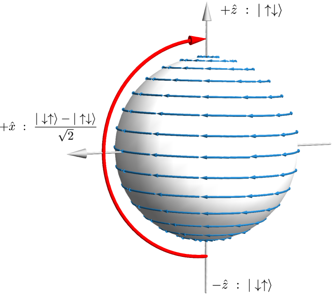
Figure 1: A simple adiabatic quantum transport: A subset of the entangled states of 2 spins form a Bloch sphere: $\cos(\theta/2)e^{i\varphi/2}\ket{\uparrow\downarrow}+\sin(\theta/2)e^{-i\varphi/2}\ket{\downarrow\uparrow}$ . The ground state of $\hat{H}=\frac{J}{2}\hat{\bm{\sigma}}_{1}\cdot\hat{\bm{\sigma}}_{2}+h(t)(\hat{\sigma}_{1}^{z}-\hat{\sigma}_{2}^{z})$ as $h(t)$ is scanned from $-\infty$ to $\infty$ follows the path shown here (red arrow), passing through a maximally entangled state. Flow fields of the $t=0$ hamiltonian are shown in blue.

The success of quantum adiabatic transport depends upon the dynamics of its entanglement resources. The simplest model of this is two coupled quantum spins-$\frac{1}{2}$. We study a simple adiabatic process of evolution under an antiferromagnetic Heisenberg model with staggered, time-dependent field:

$$H=\frac{J}{2}\bm{\hat{\sigma}}_{1}\cdot\bm{\hat{\sigma}}_{2}+h(t)(\hat{\sigma}_{1}^{z}-\hat{\sigma}_{2}^{z}).$$ (1)

The system is initialised in the state $|\uparrow\downarrow\rangle$ and the field swept from $h(0)=-\infty$ to $h(T)=\infty$. Our analysis is conveniently carried out in terms of the following parametrization of the two-spin Hilbert space:

$$\ket{\psi}=n_{1}\ket{\bm{l}_{1},\bm{l}_{2}}+n_{2}\ket{-\bm{l}_{1},-\bm{l}_{2}},$$ (2)

where the $\ket{\bm{l}_{i}}$ are spin coherent states, and $\ket{-\bm{l}_{i}}$ is the state such that $\innerproduct{\bm{l}_{i}}{-\bm{l}_{i}}=0$. The dynamics with this parametrization is particularly simple: the vectors $\bm{l}_{1}=-\bm{l}_{2}=\hat{\bm{z}}$ do not evolve and the state of the system becomes $\ket{\psi}=n_{1}\ket{\uparrow\downarrow}+n_{2}\ket{\downarrow\uparrow}\equiv\cos\theta/2\ket{\uparrow\downarrow}+e^{i\phi}\sin\theta/2\ket{\downarrow\uparrow}$, where we have represented the entanglement spinor $(n_{1},n_{2})$ as a point on a Bloch-like sphere following standard convention. In other words, the state evolves in a reduced two-dimensional subspace of the entire 4-dimensional Hilbert space – Fig. 1 shows the adiabatic path on this Bloch sphere. In the zero-magnetization subspace, the Schrödinger equation reduces to the classical equation of motion for the Bloch unit vector $\dot{\bm{n}}=\left[J\hat{x}+h(t)\hat{z}\right]\crossproduct\bm{n}.$ We can also identify a vector of operators

$$\hat{\bm{\tau}}=\begin{pmatrix}\hat{\tau_{x}}\\ \hat{\tau_{y}}\\ \hat{\tau_{z}}\end{pmatrix}=\begin{pmatrix}(\hat{\sigma}_{1}^{+}\hat{\sigma}_{2}^{-}+\hat{\sigma}_{1}^{-}\hat{\sigma}_{2}^{+})\\ -i(\hat{\sigma}_{1}^{+}\hat{\sigma}_{2}^{-}-\hat{\sigma}_{1}^{-}\hat{\sigma}_{2}^{+})\\ \ifrac{(\hat{\sigma}_{2}^{z}-\hat{\sigma}_{1}^{z})}{2}\end{pmatrix},$$ (3)

that obey $su(2)$ commutation relations, in terms of which $\hat{H}=J\left(\hat{\tau}_{x}-\hat{\tau}_{z}^{2}+\frac{1}{2}\right)-2h(t)\hat{\tau}_{z}$. In our model of adiabatic transport, the ability to sustain entanglement at the instant when $h=0$ determines whether the trajectory is connected and so whether the process is successful. We therefore investigate dynamics directly at $h=0$, i.e. $\hat{H}=J\hat{\tau}_{x}$ (for pseudospin 1/2) henceforth.

Introducing Dissipation:

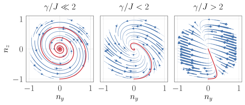
Figure 2: Flow fields and trajectories in the presence of dissipation: Blue lines show a cut through the flow fields for Eq. (5) along the $z$-$y$ plane for different dissipation strengths. Red curves indicate the fate of trajectories starting at $\ket{\uparrow\downarrow}$. $\gamma/J<2$ trajectories explore both hemispheres; $\gamma/J>2$ trajectories remain in the bottom hemisphere.

We model the environment using harmonic baths coupled locally to each spin. This assumption of locality — and the corollary that the number of dissipation channels is proportional only to the number of spins — is physically reasonable and underpins the possibility of performing quantum error correction. We consider random fields only along $\hat{z}$, motivated by systems in which different components of the qubit are of different physical origin, e.g. a flux qubit with noise arising from inductive coupling to circulating currents. If treated in a Keldysh formalism, the environment can be modelled by a random noise and a corresponding friction, resulting in a modified Schrödinger equation Crowley and Green (2016); Kamenev (2011):

$$i\partial_{t}\ket{\psi(t)} = \Big{[}\hat{H}+\sum_{i=1,2}\big{(}\eta_{i}^{z}(t)\hat{\sigma}_{i}^{z}$$

$$+\int_{0}^{t}\differential{t^{\prime}}\Gamma(t-t^{\prime})\dot{\expectationvalue{\sigma_{i}^{z}}}_{t^{\prime}}\hat{\sigma}_{i}^{z}\big{)}\Big{]}\ket{\psi(t)}.$$

Correlations in the noise fields $\eta^{z}_{i}(t)$ are related to the dissipation kernel $\Gamma(t-t^{\prime})$ by the fluctuation-dissipation relation. We study the Markovian limit $\Gamma(t-t^{\prime})=\Gamma\delta(t-t^{\prime})$. Starting from $\ket{\uparrow\downarrow}$, the $\bm{l}_{i}$ fields do not change even when coupled to the environment. The Schrödinger equation for the entanglement field reduces to

$$\dot{\bm{n}}=\left[J\hat{x}+(h(t)+\tilde{\eta}(t))\hat{z}-2\Gamma\dot{\bm{n}}\right]\crossproduct\bm{n},$$ (4)

for $\bm{n}=\langle\hat{\bm{\tau}}\rangle$. The effective noise field, $\tilde{\eta}=\eta_{1}-\eta_{2}$ has twice the variance of the local noises. Here, all stochastic differential equations should be understood as Stratonovich SDEs.

Fundamentally, it is dephasing that limits the availability of quantum resources. Friction can be systematically corrected for by applying appropriate drives or other compensating control to counter its effects. Dephasing cannot be corrected for in this way. Therefore, we will ignore the effect of friction. This amounts to a high temperature limit; $\Gamma\rightarrow 0$, $T\rightarrow\infty$, $\Gamma T\rightarrow\gamma$ finite.

The Effect of Local Dissipation:

Averaged Dynamics: The average over noise can be performed after converting Eq. (4) to an Ito SDE and allowing the state vector (now denoted $\bar{\bm{n}}$) to explore the interior of the Bloch sphere resulting in

$$\dot{\bar{\bm{n}}} =J\hat{x}\crossproduct\bar{\bm{n}}-\gamma\hat{z}\crossproduct(\bar{\bm{n}}\crossproduct\hat{z}).$$ (5)

This equation is equivalent to the Heisenberg picture Lindblad equation for the operators $\hat{\bm{\tau}}$ of Eq. (3). It has a single fixed point at the origin that is stable for all values of the coupling. This linear problem exhibits an “underdamped” to “overdamped” spectral transition in the dynamics near the fixed point at $\gamma/J=2$, as illustrated in Fig. 2. Overdamped dynamics is confined to the lower hemisphere.

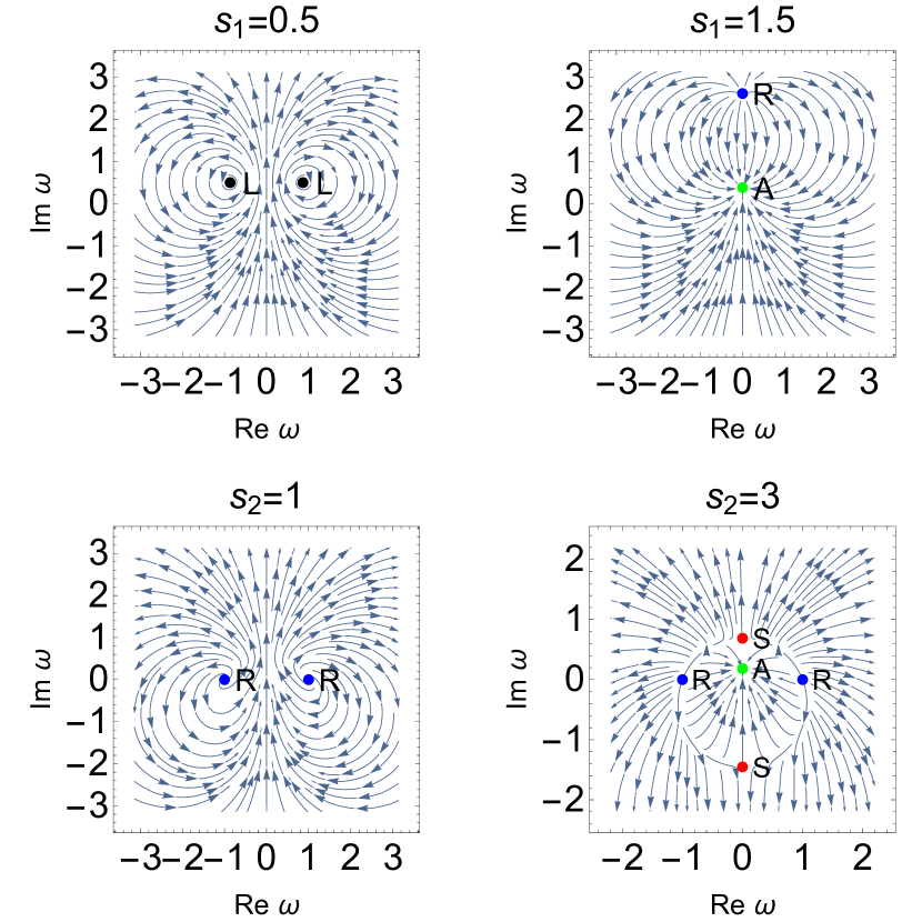
Figure 3: Environmentally induced phase space transitions – phase flows in the complex sterographic plane $w=(n_{x}+in_{y})/(1+n_{z})$
Bottom panel: Flow fields of Eq. 6 with $\gamma\to s_{2}$ (and equivalently, Eq. 15 with $s_{1}=0$) are shown in stereographic projection . For $\gamma/J<2$ there are two repulsive fixed points of this flow at $\bm{n}=\pm\hat{\bf x}$ (marked with “R” and blue color) . For $\gamma/J>2$, four new fixed points emerge, two saddles (marked with “S” and red color) and two attractors (marked with “A” and green color, the bottom one being out of field of view). The great circle through the R and S fixed points splits the Bloch sphere of Fig. 1 into two mutually inaccessible hemispheres, hence the trajectory connecting the two poles is disconnected.
Top panel: Another disconnection transition, predicted from Eq. 15 with $s_{2}=0$ – see discussion in main text for the physical realization of this transition. Formally, the similarities are due to presence/absence of the trajectory connecting the poles of the Bloch sphere on either side of the critical coupling $s_{1}/J=1$. There are, however differences in the details. In particular, instead of repulsive fixed points we find a family of periodic orbits and a pair of non-dynamical “limit” points (marked with “L”) in the small $s_{1}/J<1$ regime and only a single attractive/repulsive pair of fixed points for $s_{1}/J>1$.

Mapping to pure state dynamics: Remarkably, Eq. 5 decouples completely into radial ($d$) and angular components ($|\bm{n}|=1$), with $\bar{\bm{n}}=d\bm{n}$ and corresponding density matrix evolution

$$\dot{\bm{n}} =J\hat{x}\crossproduct\bm{n}-\gamma n_{z}\bm{n}\crossproduct\left(\hat{z}\crossproduct\bm{n}\right)$$

$$=J\hat{x}\crossproduct\bm{n}+\gamma n_{z}(\hat{\bm{z}}-n_{z}\bm{n)}$$ (6)

$$\dot{d} =-\gamma(1-n_{z}^{2}),$$ (7)

$$\hat{\rho}(t) ={\bf\hat{1}}\sqrt{1-d^{2}}+d\ \bm{n}\cdot\hat{\bm{\tau}}$$ (8)

While the radial component of the dynamics quantifies the degree of thermalization of the pseudospin $\hat{\bm{\tau}}$, angular dynamics may be thought of as describing a (non-linear) deterministic evolution of a pure state that encodes the structure of the remaining entanglement in the dimer. The spectral transition in the linear representation of the problem (Fig. 2 and Eq. 5) manifests itself in a more dramatic transition of the fixed point structure of the angular dynamics of $\bm{n}$, whose properties and physical interpretation we focus on in the remainder of this paper.

For the case considered thus far (see bottom panel of Fig. 3, with identification $\gamma\to s_{2}$) there are only two unstable (repulsive) fixed points on the underdamped side ($0<\gamma<2J$) at $\bm{n}=\pm\hat{\bf x}$. Here the trajectory of interest (see Fig.1) is the late time limiting orbit that connects the infinity ($\ket{\downarrow\uparrow}$) to the origin ($\ket{\uparrow\downarrow}$). There are six fixed points on the overdamped side ($\gamma>2J$): in addition to the (still unstable) two at $\pm\hat{\bf x}$, there are two that are stable (attractive) and two are saddles, posessing one unstable and one stable direction each. The latter four new fixed points appear in the $yz$-plane at polar angle $\theta=1/2\arcsin(-2J/\gamma)$; near $2J/\gamma=1$, they emerge at $\phi=\pi,\theta=\pi/4\pm(1-2J/\gamma)$ and $\phi=0,\theta=3\pi/4\pm(1-2J/\gamma)$. Importantly, separatracies passing from unstable points ($\pm x$) to saddles form a circular phase boundary demarkating two mutually disconnected regions of phase space as shown in Fig. 3. Hence, the trajectory starting at $\ket{\uparrow\downarrow}$ never crosses this phase boundary and rather ends up in its own attractive fixed point, i.e. it becomes “disconnected” from $\ket{\downarrow\uparrow}$ at $\gamma\geq 2J$. Top panel of Fig. 3 shows another such disconnection transition suggested by the statistical formalism we develop next.

Failure of Adiabatic Transport as a Dynamical Phase Transition:

Biased Trajectory Ensembles: in classical glasses, transitions associated with dynamical properties have been analysed in terms of ensembles of trajectories. When extended to open Hickey et al. (2012) and closed quantum systems Hickey et al. (2013), it amounts to an interpretation of the full counting statistics. The dynamical phase transition occurs as a non-analyticity in the generating function of some time-extensive order parameter. We now provide a general self-contained derivation of the large deviation formulation for our problem and demonstrate that the failure of this adiabatic process can be understood as such a transition. As a byproduct of this derivation we will also be able to identify different types of such dynamical transitions.

Consider a general initial pure state $|0\rangle$ evolving under a Hamiltonian ${\hat{H}}$ and a “biasing” perturbation ${\hat{O}}$ of strength $s$

$$\partial_{t}\ket{\psi}=\left[\hat{H}-is\hat{O}\right]\ket{\psi}.$$ (9)

We shall return to explain (below) how $\hat{O}$ (which may be generally state-dependent, i.e. nonlinear) is determined by post-selection of external measurements. Importantly, such evolution induces the loss of norm, with certain trajectories playing an amplified role compared to pure unitary evolution, hence the term biasing. One natural object to quantify this process is the conventional partition function associated with the time-evolved density matrix

$$Z_{s}(t)\equiv Tr|t\rangle\langle t|$$ (10)

$$=\langle 0|{\mathcal{T}}e^{+i\int_{0}^{t}(\hat{H}+i\frac{s}{2}\hat{O})dt^{\prime}}{\mathcal{T}}e^{-i\int_{0}^{t}(\hat{H}-i\frac{s}{2}\hat{O})dt^{\prime}}|0\rangle.$$ (11)

From here it is relatively straightforward to see that

$$\log Z_{s}(t)=-s\int_{0}^{t}\frac{\langle t^{\prime}|\hat{O}|t^{\prime}\rangle}{\langle t^{\prime}|t^{\prime}\rangle}\to-st\langle\overline{\infty}|\hat{O}|\overline{\infty}\rangle,$$ (12)

where the notation $|\bar{t}\rangle$ is used to denote a properly normalized counterpart to the time evolved state $\ket{t}$, $|\bar{t}\rangle\equiv|t\rangle/\sqrt{\langle t|t\rangle}$ with corresponding (in general nonlinear) Schrödinger equation $i\partial_{t}\ket{\bar{t}}=\left[\hat{H}-is(\hat{O}-\langle\hat{O}\rangle)\right]\ket{\bar{t}}$. We may define the dynamic quasi-free-energy functional as

$$\varphi(s)=\lim_{t\rightarrow\infty}\frac{1}{t}\ln\expectationvalue{Z_{z}(t)}\to-s\langle\hat{O}\rangle.$$ (13)

Note that we tacitly assume the existence of the (unique) steady state dominating late-time averaging in both Eqs. (12) and (13) - more on this below. The dynamics of observables can be obtained straightforwardly

$$\dot{\bm{n}}=i\langle[\hat{H}_{0},\hat{\bm{\tau}}]\rangle-\frac{s}{2}\langle\{\hat{O},\hat{\bm{\tau}}\}\rangle+s\langle\hat{O}\rangle\langle\hat{\bm{\tau}}\rangle.$$ (14)

Dephasing as Entanglement Bias:

Motivated by the observed dissipation-induced suppression of entanglement above we now consider candidate biasing operators $\hat{O}$ that may encode such an effect. Although in general the entanglement is not related to simple observables, here the pseudospin $\hat{\tau}_{z}$ is related to two standard measures of entanglement: i.  The expectation $n_{z}=\expectationvalue{\hat{\tau}_{z}}=\absolutevalue{n_{1}}^{2}-\absolutevalue{n_{2}}^{2}=\lambda_{1}^{2}-\lambda_{2}^{2}$ is the difference between the two Schmidt coefficients for the cut across the dimer; ii. The variance $\expectationvalue{\delta\hat{\tau}_{z}^{2}}\equiv\expectationvalue{(\hat{\tau}_{z}-\expectationvalue{\tau_{z}})^{2}}=1-n_{z}^{2}=2(1-\tr\rho_{A}^{2})=4\lambda_{1}^{2}\lambda_{2}^{2}$ is the concurrence Hill and Wootters (1997): a lower bound to the von Neumann entanglement entropy and an entanglement monotone ($\rho_{A}$ is the reduced density for one spin in a dimer)

We may now introduce both into Eq. 14 and find

$$\dot{\bm{n}}=J\hat{x}\crossproduct\bm{n}-s_{1}n_{z}\hat{z}\crossproduct(\hat{z}\crossproduct\bm{n})-s_{2}n_{z}\bm{n}\crossproduct(\hat{z}\crossproduct\bm{n}),$$ (15)

which is identical to Eq. (6) with $s_{1}=0$ and $s_{2}=\gamma$. We may also consider the other extreme case of $s_{2}=0$ and finite $s_{1}$ which is equivalent to the much studied non-Hermitian quantum mechanics problem Hickey et al. (2013) and to postselecting trajectories for measurements of staggered magnetization. Both of these cases can be analysed along the same lines of fixed point structure (as was already done above for the variance biased case) and dynamical free energy computed, as shown in Figs. 3 and 4. One should note that the behavior observed here is decidedely unconventional, e.g. we observe a “zeroth order transition” in the variance biased case. Importantly, late time averages necessary to compute $\varphi$ are not straightforward. The underdamped regime does not possess an attractive fixed point so $n_{z}=0$ results from integrating over a persistent oscillation. In the overdamped regime of the variance biased case, there are two attractors (bistability). The attractor reached from the South pole of Fig. 1 (located below the field of view displayed in the bottom-right panel of Fig. 3) is of interest here, resulting in the discontinuous behavior of $\varphi$ in Fig. 4.

a)                                  b)                            

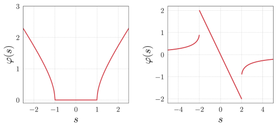
Figure 4: Dynamical free energy with entanglement bias (J=1): The dynamical free energy for the Heisenberg model a) with linear bias corresponding to $s_{1}=s$ and $s_{2}=0$ in Eq. (15), and b) with variance bias corresponding to $s_{1}=0$ and $s_{2}=s$ in Eq. (15). The variance-biased cumulant generating function b) exhibits a dynamical phase transition at $\ifrac{s}{J}=2$, signifying the failure of the adiabatic process. The linear biased cumulant generating function a) exhibits a non-analyticity at $s/J=1$, another signature of this failure.

Conclusion:

Dephasing biases quantum trajectories and restricts the accessible regions of Hilbert space to those with low entanglement. This can induce the failure of adiabatic quantum computation — where intermediate states in the computation are typically highly entangled — and of quantum control. It is mirrored in recent studies of restriction of entanglement growth in random circuits with weak or projective measurement Li et al. (2018); Skinner et al. (2019); Chan et al. (2019). We have given a concrete demonstration that — for a simple adiabatic process in a system of two quantum spins — this failure of adiabatic transport is a dynamical phase transition. Within a trajectory ensemble treatment, the transition is accompanied by a discontinuity in the scaled cumulant generating function associated with a time extensive order parameter. The order parameter is related to the entanglement structure of the system.

Our model can be realised directly in coupled flux qubits. The environmental noise in such a system is often dominated by flux noise that corresponds to effective noise fields in the z-direction only Crowley and Green (2016). An intriguing alternative is to realise the non-linear Schrödinger evolution of Eq. (9) using a post-selection scheme You et al. (2020a). The situation that we have described effectively biases the qubit dynamics with the variance of an operator rather than simply an operator as in the usual linear bias cases. This necessitates a greater degree of post-selection corresponding to the additional tomography required to find the variance of the operator at each time-step or the image of this in measurements carried out on the bath Hickey et al. (2013).

Can this analysis can be extended to many spins and to true adiabatic quantum computation? Quantum advantage requires as many as fifty coherent spins, and a useful paradigm for understanding computational failure must generalise to such systems. There are some hints that the ideas presented here can be extended successfully. Recent analysis of sweeps through a topological phase transition in the presence of an external bath reveal the same equations as Eq. (6) albeit in a system of non-interacting particles You et al. (2020b). It is also possible to extend the Langevin approach used here to study more profoundly entangled many body systems Morley-Wilkinson (2019) within a matrix product state Langevin description. A typical adiabatic computation undergoes several avoided crossings of low-lying levels. The states at the avoided crossings are often highly entangled. Environmental depletion of entanglement can thus prevent the avoided crossing and cause a failure of the computation. Thresholds for error correction in gate based models of quantum computation do not currently have an analogue in adiabatic computation. Our hope is that mapping the failure of adiabatic transport to a dynamical phase transition will prove useful in this search.

Acknowledgements: We thank S. Gopalakrishnan and E. Kapit for useful discussions of ideas explored in this work. VO acknowledges support from the NSF DMR Grant No. 1508538. AGG and FB acknowledge support from the EPSRC.

References

- Born and Fock (1928) M. Born and V. Fock, Zeitschrift für Physik 51, 165 (1928), ISSN 0044-3328, URL https://doi.org/10.1007/BF01343193.
- Bergmann et al. (1998) K. Bergmann, H. Theuer, and B. W. Shore, Rev. Mod. Phys. 70, 1003 (1998), URL https://link.aps.org/doi/10.1103/RevModPhys.70.1003.
- Kadowaki and Nishimori (1998) T. Kadowaki and H. Nishimori, Physical Review E 58, 5355 (1998).
- Brooke (1999) J. Brooke, Science 284, 779 (1999).
- Farhi et al. (2001) E. Farhi, J. Goldstone, S. Gutmann, J. Lapan, A. Lundgren, and D. Preda, Science 292, 472 (2001).
- Santoro et al. (2002) G. E. Santoro, R. Martoňák, E. Tosatti, and R. Car, Science 295, 2427 (2002).
- Aharonov et al. (2008) D. Aharonov, W. Van Dam, J. Kempe, Z. Landau, S. Lloyd, and O. Regev, SIAM review 50, 755 (2008).
- Altshuler et al. (2010) B. Altshuler, H. Krovi, and J. Roland, Proceedings of the National Academy of Sciences 107, 12446 (2010), ISSN 0027-8424, URL http://www.pnas.org/content/107/28/12446.
- Jörg et al. (2010) T. Jörg, F. Krzakala, G. Semerjian, and F. Zamponi, Phys. Rev. Lett. 104, 207206 (2010), URL https://link.aps.org/doi/10.1103/PhysRevLett.104.207206.
- Laumann et al. (2015) C. R. Laumann, R. Moessner, A. Scardicchio, and S. Sondhi, The European Physical Journal Special Topics 224, 75 (2015).
- Denchev et al. (2016) V. S. Denchev, S. Boixo, S. V. Isakov, N. Ding, R. Babbush, V. Smelyanskiy, J. Martinis, and H. Neven, Physical Review X 6, 1 (2016), ISSN 21603308, eprint 1512.02206.
- Crowley et al. (2014) P. J. D. Crowley, T. Duric, W. Vinci, P. A. Warburton, and A. G. Green, Physical Review A 042317, 1 (2014).
- Bauer et al. (2015) B. Bauer, L. Wang, I. Pižorn, and M. Troyer (2015), URL https://www.microsoft.com/en-us/research/publication/entanglement-resource-adiabatic-quantum-optimization/.
- Wild et al. (2016) D. S. Wild, S. Gopalakrishnan, M. Knap, N. Y. Yao, and M. D. Lukin, Physical review letters 117, 150501 (2016).
- Aharonov and Ben-Or (2008) D. Aharonov and M. Ben-Or, SIAM Journal on Computing 38, 1207 (2008), URL https://doi.org/10.1137/S0097539799359385.
- Jordan et al. (2006) S. P. Jordan, E. Farhi, and P. W. Shor, Physical Review A 74, 052322 (2006).
- Young et al. (2013) K. C. Young, M. Sarovar, and R. Blume-Kohout, Physical Review X 3, 041013 (2013).
- Pudenz et al. (2014) K. L. Pudenz, T. Albash, and D. A. Lidar, Nature communications 5, 1 (2014).
- Crowley and Green (2016) P. J. D. Crowley and A. G. Green, Physical Review A 94, 1 (2016), ISSN 24699934.
- Kamenev (2011) A. Kamenev, Field theory of non-equilibrium systems (Cambridge University Press, 2011).
- Hickey et al. (2012) J. M. Hickey, S. Genway, I. Lesanovsky, and J. P. Garrahan, Physical Review A - Atomic, Molecular, and Optical Physics 063824, 1 (2012).
- Hickey et al. (2013) J. M. Hickey, S. Genway, I. Lesanovsky, and J. P. Garrahan, Physical Review B - Condensed Matter and Materials Physics 87, 1 (2013), ISSN 10980121, eprint 1211.4773.
- Hill and Wootters (1997) S. Hill and W. K. Wootters, Physical Review Letters 78, 5022 (1997), ISSN 10797114, eprint 9703041.
- Li et al. (2018) Y. Li, X. Chen, and M. P. Fisher, Physical Review B 98, 205136 (2018).
- Skinner et al. (2019) B. Skinner, J. Ruhman, and A. Nahum, Physical Review X 9, 031009 (2019).
- Chan et al. (2019) A. Chan, R. M. Nandkishore, M. Pretko, and G. Smith, Physical Review B 99, 224307 (2019).
- You et al. (2020a) Y.-Z. You, W.-T. Kuo, D. Arovas, and S. Vishveshwara, Perimeter Quantum Frontiers Seminar (2020a).
- You et al. (2020b) Y.-Z. You, W.-T. Kuo, D. Arovas, and S. Vishveshwara, Decoherent quench acros quantum phase transitions, http://pirsa.org/20110004 (2020b).
- Morley-Wilkinson (2019) J. G. Morley-Wilkinson, Ph.D. thesis, UCL (University College London) (2019).