Randomly repeated measurements on quantum systems:
Correlations and topological invariants of the quantum evolution
K. Ziegler1, E. Barkai2 and D. Kessler31Institut für Physik, Universität Augsburg, D-86135 Augsburg, Germany
2Department of Physics, Institute of Nanotechnology and Advanced Materials,
Bar-Ilan University, Ramat Gan 52900, Israel
3Department of Physics, Bar-Ilan University, Ramat Gan 52900, Israel
Abstract
Randomly repeated measurements during the evolution of a closed quantum system
create a sequence of probabilities for the first detection of a certain quantum state.
The related discrete monitored evolution for the return of the quantum system
to its initial state is investigated. We found that the mean number of measurements
until the first detection is an integer, namely the dimensionality of
the accessible Hilbert space. Moreover, the mean first detected return time is equal to
the average time step between successive measurements times the mean number of measurements.
Thus, the mean first detected return time scales linearly with the dimensionality of the
accessible Hilbert space. The main goal of this work is to explain the quantization
of the mean return time in terms of a quantized Berry phase.
I Introduction
The unitary evolution (UE) of a closed quantum system from the initial state to the state
on the time interval is defined by ,
where is the Hamiltonian of the system. The result of this
evolution is characterized by the overlap amplitude with respect to a given state .
Then is the probability that the evolution has reached the state ,
which obviously depends on the time .
In a single experiment the measurement time is fixed and, therefore, the UE
allows us to detect the state with probability only once.
The detection of this state at different times
would require the repetition of the experiment, prepared in the same initial state , for different values of
[1].
An alternative approach, which we call “monitored evolution (ME)” is to allow the system to evolve from the initial state
for the time
and then measure whether or not the system is in the state . If the answer is “yes”, we stop
the experiment, if the answer is “no” we allow the system to evolve further after the measurement [2]
and perform a second measurement at time . This procedure is repeated for times
, …, until the measurement detects the state for the first time.
We consider cases in which the state is detected with probability one. This is called a recurrent measurement process
[1].
If at time the outcome of the measurement is null this
can be associated with a projection of the quantum system with a
subsequent normalization of the resulting state [3], and similarly for etc.
And when the state is detected for the first time at time , the amplitude of the corresponding state is
and its probability is [4, 5].
For fixed time steps with the repeated measurement approach, also known as the stroboscopic protocol,
has been studied in great detail in Refs. [1] and
[6, 7, 8, 9, 10, 11, 4, 5, 12, 13, 3, 14, 15, 16, 17, 18, 19].
Two cases have been distinguished, the return
probability for and the transition probability for .
It was found that
(i) the return and the transition probabilities differ qualitatively,
(ii) the average first detected return time is quantized and given by the winding number of the Laplace transform of
the return amplitude [1],
(iii) near degeneracies of the spectrum of the evolution operator, the fluctuations become very large and diverge at the
degeneracies [11, 3, 18],
and (iv) the average first detected transition time also diverges at the degeneracies [20].
Our main intention is to present in this article a study of the effect of independent and identically
distributed random time steps on the ME. For this purpose we want to answer the following questions:
(1) Do we still obtain quantization of the number of attempts for the first successful measurement?
(2) Is the average mean time for the first detection also quantized, as found for stroboscopic measurements?
(3) How can dynamical quantization be related to topological invariants?
(4) Do random time steps affect the divergent fluctuations near resonances?
To answer these questions we will develop a theory of the first detection time under repeated random measurements.
Our work is based on the ideas presented by Grünbaum et al. [9] for fixed time steps and related
to a work by Varbanov et al. [21] on random time steps, who studied the conditions for the existence
of non-detectable dark states.
Random time measurements were discussed also for open quantum systems [22], while
for closed quantum systems they were recently studied by us in terms of average return and transition
probabilities [PhysRevA.103.022222]. The present work is an extension of the latter in which we explain in
detail the origin of the quantization of the mean return time. For this purpose we compare the Berry phase
of the return amplitude, averaged with respect to the distribution of the measurement times. It will be
shown that the average Berry phase is equal to the average number of measurements for the first detected return
and equal to the dimensionality of the accessible Hilbert space. The average Berry phase is reminiscent of the quantized
winding number in case of stroboscopic measurements [9].
The structure of this article is as follows.
In Sect. II the definitions of the relevant quantities for the first detection under repeated
measurements are given.
Then a short summary of the main results are presented in Sect. III.
After a brief discussion of the ME for fixed time steps
in Sect. IV, we formulate the ME for random time steps in terms of random matrix products
in Sects. V-VI.2.1. This includes a description of the averaging procedure
(Sect. VI) and the introduction of a generating function for the average return
time and its higher moments (Sect. VI.1). The quantization of the mean number of measurements of the
first detected return by the dimensionality of the accessible Hilbert space is studied in Sects. VI.2
and VI.2.1.
Finally, in Sect. VII the example of a symmetric two-level system is analyzed, followed by a discussion of
all the results in Sect. VIII.
Details of the calculations are presented in Apps. A-F.
II Return amplitude of the monitored evolution
The return probability as a function of time, with or without intermediate measurements, provides a measure of how big the
accessible space is and how long it takes to return to the initial state. This is an important
quantity for classical random walks [23, 24] and plays also an important role
for characterizing localization in many-body quantum systems [25, 26].
We will investigate the return amplitude for the ME with measurements at time steps .
First, we will have need to refer to the return amplitude of the UE
(1)
for the state when we measure only once after the time ,
assuming that the UE is governed by the Hamiltonian .
Then we turn to the return amplitude for the ME [4, 13, 3]
(2)
which is the major objective of our inquiry.
This is the return amplitude at time , provided that we also measure at times
but detect the quantum state for the first time at with probability .
For the time of measurements we assume a distribution density of independent and identically
distributed time steps, such that .
This can be understood as the effect of an inaccurate clock.
This enables us to consider the average
with respect to the ensemble of random time steps. Here we do not specify the distribution.
For instance, can be a Dirac delta, which would recover the
stroboscopic ME [9, 13, 3, 18], it could be an exponential distribution
or any other distribution, which allows us to perform the average .
Besides the averaging with respect to times steps we also need to define the averages
(3)
Here it is assumed that , which is justified for a finite-dimensional Hilbert space
(cf. App. A). This equation means that the state is eventually detected [9].
Thus, the overline represents a double average, namely
an average with respect to the number of time steps with weight , followed by
the average .
For both expressions in Eq. (3) will be used to characterize the ME:
is the mean number of measurements for the first detected return (FDR) and is the mean FDR time.
Since both evolutions are defined on an -dimensional Hilbert space
by the Hamiltonian , we consider its eigenstates and its
corresponding eigenvalues .
Then the return amplitude of the ME can be expressed as a matrix product, which is efficiently
written in the energy representation as a sum over all energy levels as
(4)
In principle, there is the possibility of degenerate eigenvalues or of a vanishing overlap
, which must be treated with care [9].
To understand the effect of degenerate energy levels on we consider the levels , and
assume at first that they are not degenerate. Then we can write
where the second term on the right-hand side describes the evolution of the state
with the evolution operator
over the time period . The evolution creates a superposition of the states and ,
which changes in time due to the time dependent coefficients, provided that . On the other
hand, for the degenerate case , the superposition of and
is fixed during the time period :
and only the global phase changes. This reflects a dimensional reduction of the accessible Hilbert space by 1,
implying that we should use the replacement
and the simultaneous elimination of from the summation of in Eq. (4).
Another special case is a vanishing overlap .
Beginning with the initial state on the right-hand side of Eq. (4) we get
Next, in the summation with respect to the special value does not contribute again,
since gives
due to and due to .
Repeating this argument we find that the value drops out of all summations in Eq. (4),
reducing the accessible Hilbert space by 1 again.
With these arguments we have removed the degeneracy of the energy levels and the vanishing overlaps .
Therefore, the remaining return amplitude depends only non-degenerate energy levels and on overlaps with .
For the subsequent analysis we use the convention that is the dimensionality of the accessible Hilbert space.
For the subsequent calculations it is useful to introduce
two types of discrete Fourier transformations, where one is based on the phase factors
(5)
and the other is based on the random phase factors
(6)
provided that these series exist. Both and are still functions
of the random variables .
III Summary and Results
It will be shown that for a quantum system with energy levels and eigenstates of
a given Hamiltonian
the FDR probability in the case of a ME is determined by the random phase factors
and the overlaps alone. After averaging with
respect to the random measurements we get , which will turn out to be a function of
the parameters and of the parameters
. (Details are given in Sect. V.)
Using the Fourier transformations (5) and (6), we define the generating functions
and .
By differentation with respect to we get the mean number of measurements for the FDR and the mean
FDR time as
Then we will derive the relation , where
is the mean time interval between successive measurements.
Besides the average FDR probability we will also calculate the corresponding
expressions of the Fourier transform , namely .
This will turn out to be 1, as shown in Eq. (33), which is
essential for calculating the average Berry phase and the mean values of the FDR as
In this section we briefly recapitulate what is known about the FDR problem in the case of
non-random to set the stage for our investigation of random time steps .
Stroboscopic measurement with has been studied extensively in the
literature [9, 11, 13, 3, 14, 18].
Next we summarize relevant information from previous works, in particular,
some results of Ref. [18].
At fixed the Laplace transformation for the return amplitude of the ME reads
(8)
Due to the relation of Eq. (53) in App. B,
we obtain for the following identity
(9)
This identity is important because it allows us to represent the projector-dependent left-hand side
by the expression , which is diagonal in terms of the energy
eigenstates of and independent of the projector . A corresponding
identity exists in the case of random time steps, which will be central for our subsequent calculations.
With of Eq. (1) we can write
as the Laplace transform of : .
Then in Eq. (8), together with Eq. (9), becomes
(10)
By analytic continuation to the unit circle we get
and .
Since , the expression is unimodular:
(11)
such that we can write
(12)
This result for fixed time steps indicates that the UE and the ME have the same phase change with except for a
factor 2.
The winding number of around the unit circle (i.e. for ) is identical with
, and it is known that the winding number is equal to the dimensionality of the Hilbert space [9].
V Matrix products
Our goal is to calculate the probability
of the return amplitude of Eq. (4) for the general case of random time steps.
We would expect that the calculations of the previous section can be extended to this situation. As we will see though
it requires some additional steps to calculate quantities, such as the mean FDR time, that are averaged with respect to the
random time steps.
Our calculation starts with the matrix representation of the projector of Eq. (2) in terms of energy
eigenstates
(13)
since the eigenstates are orthonormal: .
This is automatically fulfilled for non-degenerate eigenvalues.
The above expression is inserted in Eq. (4) and yields for
the return amplitude a trace of a matrix product:
with the matrix , whose elements are all 1, and with the
diagonal matrices
and .
Now is the diagonal matrix , which enables us to rewrite as
(14)
since and as diagonal matrices commute.
This means that depends only on the spectral weights through and on the energy
levels through .
For the calculation of the return probability we need the product of two traces
(15)
In order to express this product it is convenient to use the notation of the Kronecker product of matrices
with the properties
(16)
The second identity, or trace “disentanglement” relation, is relevant for Eq. (15).
With the matrix
it gives us
(17)
with , and .
For the matrix elements we use the notation
(18)
VI Averaging over the distribution of random time steps
In the previous section we obtained a random distribution of return probabilities .
Here we are interested in the mean values ,
The subsequent calculation of the time average is based on the fact that the random
matrices are statistically independent and identically distributed. Thus, from
Eq. (17) we get
(19)
With the matrices
(20)
and
(21)
we obtain the compact expression
(22)
depends on the averaged product .
The latter cannot be expressed as a Kronecker product, which prevents us also from applying the trace
”disentanglement” relation of Eq. (16). This reflects a robust “entanglement” due to
. We will return to this fact in the next section.
VI.1 The generating functions
First, from Eq. (22) we obtain, after a discrete Fourier transformation, the generating functions
(23)
and
(24)
with
(25)
and
(26)
As shown in App. E, the matrix is analytic for .
This means that we should consider the discrete Fourier summation as an analytic continuation
from .
From and we can calculate moments of and with
respect to the weight and , respectively, as
(27)
The property , discussed in App. A, indicates a close relation between the
two generating functions. Then the dependence of the generating functions is through the fact that
(i) and depend on only through
and , respectively,
and (ii) the matrix is a function of .
It implies that we can replace a derivative with respect to by a derivative with respect to the difference of
energy levels if (). Since the latter is implicitly assumed here for all energy levels,
we can write for the first moment in Eq. (27)
with .
The first sum on the right-hand side vanishes due to and consequently ,
such that we obtain
(28)
The analog calculation is valid for and gives
(29)
Comparing the expressions in Eqs. (28) and (29) implies
for the first moments in Eq. (27) the relation
(30)
VI.2 Evaluation of
Next we will show that holds in general for any integer due to
(31)
where was defined in Sect. V.
To derive this property and to calculate the mean FDR time we use the matrix relations
(32)
where is the diagonal matrix , and
is a sequence of zeros. is the diagonal matrix with elements
of Eq. (31).
The contribution on the right-hand side disappears,
since .
The first relation of Eq. (32) is obtained from
by a direct inspection of the matrix elements:
and the second relation for from
Provided that the inverse of exists,
the second relation of Eq. (32) implies
, which
gives directly Eq. (31) and subsequently the normalization
(33)
according to Eq. (65) of App. D.
This result can be used to reduce the integral of the average winding number
(34)
which is discussed in more detail in Sect. VIII,
with the help of Eq. (33) to
(35)
In the next section we will see that is an integer, equal to the dimensionality of
the accessible Hilbert space.
VI.2.1 Mean FDR time
Now we return to the first moment in Eq. (27), using an extension of the previous calculation.
Starting with
(36)
we write for the matrix inside the trace
and apply the first relation of Eq. (32) to the first inverse matrix to obtain
(37)
where the last equation is due to .
This can be inserted into Eq. (36), and with the second relation of Eq. (32) we get
(38)
where the last two equations follow from Eq. (31) and the definition of .
This result gives us, together with Eqs. (30) and (38),
for the mean number of measurements (MNM) of the FDR and the mean FDR time
(39)
which presents an extension of a central result of the seminal work by Grünbaum et al. [9]
of stroboscopic measurements to random time measurements.
As already mentioned in the Introduction, higher order moments are not quantized but can be very sensitive to degeneracies
of the spectrum, at least for stroboscopic measurements[11, 3, 18].
In the case of random measurements this is also true near degeneracies of the energy levels when
() is close to 1.
This originates in the fact that for
small eigenvalues of can appear.
This can indeed happen when at least one is close to 1 or when one is
close to 0, as shown in App. E.
VII Example: symmetric two-level system
In the previous section we derived relations between the MNM of the FDR and the mean FDR time,
their relation with the average winding number of Eq. (34)
and with the dimensionality of the Hilbert space in Eq. (39).
These results are general and valid for any quantum system on an –dimensional Hilbert space. Besides these mean
values we obtained in Eq. (27) also higher moments of the number of measurements and the return time for the FDR.
For we have not found a simple expression but can obtain these moments only by calculating the
generating functions and directly. To determine these generating functions would require
the inversion of the matrix . This is a tedious task, which goes beyond the scope
of this paper. Therefore, we limit ourselves to and calculate the corresponding matrices
(cf. App. F). In particular,
we consider a symmetric two-level system (2LS) with energy levels and spectral weights
for random times. The Hilbert space is two-dimensional with two basis states, e.g.
and . If the measured state is , the projector reads .
Then we get and and the
return amplitude reads
(40)
The simplicity of the two-level system is manifested in the fact that is a scalar product
in contrast to the matrix product in Eq. (14) of the general case . This
simplifies calculations with respect to random substantially. For instance, we can easily
perform the summation with respect to to get
(41)
as a special case of the general equation (50).
After averaging with respect to , we get for the mean FDR time
(42)
which is in agreement with our general result in Eq. (39).
Moreover, the generating functions in Eq. (23) and
in Eq. (24) read
(43)
which gives for
(44)
where the first equation reflects the normalization, the second equation the quantization of the mean FDR time and the
last equation the FDR fluctuations. The latter only diverge for in the case of random times steps, but
in the case of a fixed time step it also diverges for () . For we get
(45)
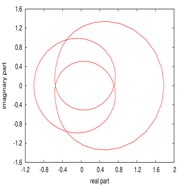
The two-level systems gives also a direct insight into the effect of random time steps
on the return amplitude before averaging, since we can calculate these amplitudes
from Eq. (40) for special realizations of . A few examples are visualized in Fig.
1, indicating that as well as the winding number vary from realization
to realization substantially.
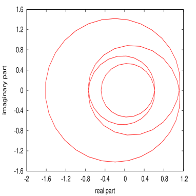
For fixed time steps, on the other hand, we have and the
winding number is 2 in Fig. 2, as predicted by the general theory of stroboscopic
measurements [9, 18].
Figure 1:
Symmetric two-level system:
The return amplitude
on the interval
with three randomly chosen realizations of performs a closed trajectory in the
complex plane. The winding numbers in these examples are , respectively.
Figure 2:
Symmetric two-level system:
The return amplitude
on the interval with fixed time step .
The winding number in this example is .
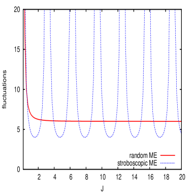
Figure 3:
Symmetric two-level system: Fluctuations of the FDR for stroboscopic ME and random time steps
from Eqs. (48) and (49).
VIII Discussion
The aim of our work has been to calculate the properties of the ME with random measurements through the return
amplitude .
For given eigenvalues and eigenstates of the Hamiltonian
the ME of the return to the initial state are characterized by the time averaged phase factors
, and by the spectral
weights . This allowed us to calculated the mean FDR times and the MNM of the FDR, using
the generating functions defined in Eqs. (23) and (24).
The surprising result in Eq. (39) is that the MNM of the FDR is just the dimensionality
of the accessible
Hilbert space and that the mean FDR time is , where
is the mean time between two successive measurements.
The same was previously observed for fixed time steps [9, 11, 18].
The robustness of the average winding number is remarkable, since the winding number of the return amplitude
fluctuates strongly from realization to realization of the random (cf. Fig. 1).
Other quantities, such as the correlation function
of the return amplitudes for different discrete times and in Eq. (57), can also be calculated.
An example is , which is 1
according to the calculation in App. D. This enabled us to determine the mean FDR time
in Eq. (39).
Its connection with the integral in Eq. (34) is a generalization of the quantized
winding number in the case of stroboscopic measurements by Grünbaum et al. [9, 18].
The latter is based on the fact that (cf. Eq.(12)). Then the winding number
simply reads for (cf. Ref. [3] and Sect. IV)
In the case of random time measurements , such that we must modify the definition
of the winding number by normalizing .
A further problem is that the winding number depends on the realization of the time steps , as we have
demonstrated in Fig. 1 for the symmetric two-level system. Therefore, we must also perform an average
with respect to the time steps. Then the definition of the winding number becomes Eq. (34),
which reads with as an average differential phase
change
(46)
Here we note that Eq. (34) is formally equivalent to the definition of the Berry phase [27]
when we replace by the spatial wave function and replace the
time average by the usual quantum average in space.
Averaging over random time steps is crucial to obtain a generic winding number.
That different special realizations of the random time steps lead to different winding numbers can be seen
when we assume a finite sequence of (). The latter is either the result of an
approximative truncation of the sequence or when the sequence terminates with in Eq. (50).
Then the Fourier transformed return amplitude in Eq. (5) becomes a finite sum
for which a winding number can be defined for (random) coefficients as
(47)
Then we rewrite the polynomial as the product
such that we get for the winding number
With this gives
where the Cauchy integral is performed over the unit circle and () is the number of
poles inside the unit circle. A simple example is with
where we get
A detailed calculation of several quantities was presented in Sect. VII for
the case of a symmetric two-level system with after averaging with respect to .
The fluctuations of the return time are finite
(48)
where the last expression is obtained from the Poisson distribution .
In the limit of a fixed measurement time the fluctuations
(49)
would diverge for ().
Thus, the random measurements wash out the divergences of the fluctuations. For most values of the level splitting
the fluctuations are stronger for the fixed time steps, as visualized in Fig. 3.
In this paper we have completely focused on the return of the quantum system to its initial state. A natural
extension would be a corresponding analysis of the transition from an initial to a different final state,
monitored by random projective measurements. We have addressed this topic in a separate article [PhysRevA.103.022222].
In conclusion, the mean FDR time of the ME for random time steps is equal to the dimensionality of the accessible
Hilbert space. This is very similar to the ME for fixed time steps.
On the other hand, the strong fluctuations of the FDR time, which appear for a small distance of eigenvalues
in the case of fixed time steps, are washed out by averaging with respect to the random time steps. This was
briefly discussed for a two-level system in this article and more general in Ref. [PhysRevA.103.022222].
SME
RME
probability
random
probability
winding number of
random
winding number of
mean number of measurements for FDR
mean FDR time
Table 1: Comparison between stroboscopic ME (SME) and random ME (RME) with the Hilbert space dimensionality .
The first detected return agrees for both approaches, provided that we average over the random measurements.
Acknowledgments:
The support of Israel Science Foundation’s Grant No. 1898/17 as well as the support by the Julian
Schwinger Foundation (K.Z.) are acknowledged.
Appendix A Normalization
The normalization of the vector with
in the limit is based on the normalization of
and will be derived by iteration:
For the evaluation of we consider the sequence of projection operators with
With and we can insert at
Next we replace in the second term by
to get
The replacement of the operator by
can be repeated for to obtain
where
Thus, we have
(50)
where the probability of not recording the state after attempts is
Provided the remainder vanishes in the limit , the wave function
is normalized in this limit: .
Although we do not have proof that always vanishes with , the latter is plausible
and is supported by the example of the symmetric two-level system in Eq. (41),
by stroboscopic measurements [9] and in the case of the time averaged sum
[PhysRevA.103.022222].
Appendix B Recursion
For an operator and the projector we assume that the
inverse exists. Then we get the relation
and
.
This allows us to write for the Fourier transform of Eq. (57)
(63)
with
(64)
These are analytic functions in and , respectively, and their special form implies .
For the normalization can be obtained
from Eq. (63) with the help of Eq. (31). This can be shown by the following reasoning.
From App. A we have . Then we can write with Eq. (63)
(65)
Inserting now from Eq. (31) and use
we obtain 1 for this expression.
Now we introduce the projector with . Then we can write
and since
(69)
The eigenvalues of might be complex. Therefore, it is better to calculate the
eigenvalues of the Hermitean matrix
whose determinant reads
(70)
A necessary condition for a quick decay of with is that
the product of is not small, while the sufficient condition
requires that also is not small.
To see the latter, we analyze the elements of the projected matrix
(71)
We only consider the projected matrix, which has the following matrix elements with
and :
and
For the special case of this gives a matrix:
whose determinant vanishes only for and/or .
Appendix F Symmetric two-level system
The matrix structure of the symmetric 2LS reads
and
Then we have
with . Moreover,
such that
with three vanishing eigenvalues and one eigenvalue .
With the help of Maxima we obtain with
Friedman et al. [2017]H. Friedman, D. A. Kessler, and E. Barkai, Quantum walks: The first
detected passage time problem, Phys. Rev. E 95, 032141 (2017).
Dhar et al. [2015a]S. Dhar, S. Dasgupta,
A. Dhar, and D. Sen, Detection of a quantum particle on a lattice under
repeated projective measurements, Phys. Rev. A 91, 062115 (2015a).
Krapivsky et al. [2014]P. Krapivsky, J. Luck, and K. Mallick, Survival of classical and quantum
particles in the presence of traps, J Stat Phys 154, 1430 (2014).
Sinkovicz et al. [2016]P. Sinkovicz, T. Kiss, and J. K. Asbóth, Generalized kac lemma for recurrence
time in iterated open quantum systems, Phys. Rev. A 93, 050101 (2016).
Thiel et al. [2018]F. Thiel, E. Barkai, and D. A. Kessler, First detected arrival of a quantum
walker on an infinite line, Phys. Rev. Lett. 120, 040502 (2018).
Lahiri and Dhar [2019]S. Lahiri and A. Dhar, Return to the origin problem for a
particle on a one-dimensional lattice with quasi-zeno dynamics, Phys. Rev. A 99, 012101 (2019).
Yin et al. [2019]R. Yin, K. Ziegler,
F. Thiel, and E. Barkai, Large fluctuations of the first detected quantum return
time, Phys. Rev. Research 1, 033086 (2019).
Dubey et al. [2020]V. Dubey, C. Bernardin, and A. Dhar, Quantum Dynamics under
continuous projective measurements: non-Hermitian description and the
continuous space space limit, arXiv e-prints , arXiv:2012.01196
(2020), arXiv:2012.01196 [quant-ph] .
Liu et al. [2020]Q. Liu, R. Yin, K. Ziegler, and E. Barkai, Quantum walks: The mean first detected transition time, Phys. Rev. Research 2, 033113 (2020).
Varbanov et al. [2008]M. Varbanov, H. Krovi, and T. A. Brun, Hitting time for the continuous
quantum walk, Phys. Rev. A 78, 022324 (2008).
Riera-Campeny et al. [2020]A. Riera-Campeny, J. Ollé, and A. Masó-Puigdellosas, Measurement-induced resetting in open quantum systems, arXiv e-prints , arXiv:2011.04403 (2020), arXiv:2011.04403 [quant-ph] .