Chiral separation effect catalyzed by heavy impurities

Abstract

We investigate the influence of Kondo effect, namely, the nonperturbative effect induced by heavy impurities, on the chiral separation effect (CSE) in quark matter. We employ a simple effective model incorporating the Kondo condensate made of a light quark and a heavy quark, and compute the response function of axial current to the magnetic field in static limit and dynamical limit. As a result, we find that the Kondo effect catalyzes the CSE in both the limits, and particularly the CSE in dynamical limit can be enhanced by a factor of approximately three. Our findings clearly show that the presence of heavy impurities in quark matter can play an important role in the transport phenomena of light quarks induced by a magnetic field.

I Introduction

Investigation of currents induced by an external magnetic field is one of the most important subjects in association with heavy-ion collision (HIC) and neutron star (NS) physics. For example, it was proposed that a magnetic field applied in chirality imbalanced matter gives rise to a vector current, which is called the chiral magnetic effect (CME) Kharzeev (2006); Kharzeev and Zhitnitsky (2007); Kharzeev et al. (2008); Fukushima et al. (2008) (see also Ref. Vilenkin (1980a); Nielsen and Ninomiya (1983) for earlier works). Another example is the chiral separation effect (CSE) Son and Zhitnitsky (2004); Metlitski and Zhitnitsky (2005); Newman and Son (2006) which refers to an axial current induced by a magnetic field in ordinary baryonic or quark matter. The CME has been mostly studied with respect to high-energy HICs in which a chirality imbalanced environment may be created by metastable states related to the $\theta$-vacua Kharzeev et al. (1998); Kharzeev and Pisarski (2000); Kharzeev et al. (2002). The CSE is expected to play an important role in low-energy HICs in which finite baryon density can be created, as well as in NSs.

In quark matter, in addition to light quarks ($u,d$) with the Fermi surface, heavy quarks ($c$) may exist as impurities. In such a situation, light quarks near the Fermi surface can be correlated with the heavy quarks in a nonperturbative way due to the non-Abelian interaction with $SU(N_{c})$ symmetry ($N_{c}$ is the number of colors) of quantum chromodynamics (QCD). As a result, a condensate made of a light quark and a heavy quark is created, which is the so-called Kondo condensate. The emergence of Kondo condensate and phenomena induced by the condensate are called Kondo effect. While the Kondo effect was originally found in metal including impurities in the context of condensed-matter physics Kondo (1964); Hewson (1993); Yosida (1996); Yamada (2004); Coleman (2015), it has been theoretically shown to emerge in quark matter Yasui and Sudoh (2013); Hattori et al. (2015) (See Refs. Ozaki et al. (2016); Yasui et al. (2019); Yasui (2017); Kanazawa and Uchino (2016); Kimura and Ozaki (2017); Yasui and Ozaki (2017); Suzuki et al. (2017); Yasui et al. (2017); Kimura and Ozaki (2019); Fariello et al. (2019); Hattori et al. (2019); Suenaga et al. (2020a, b); Kanazawa (2020); Araki et al. ; Araki et al. (2020); Kimura (2020) for related discussions).

The Kondo effect is known to change the transport phenomena characteristically. For example, this effect tends to suppress the electric conductivity of charged particles as we lower the temperature. Similarly, we expect that the Kondo effect also influences the transport phenomena induced by a magnetic field. Based on this expectation, in this paper we discuss modification of CSE due to the Kondo effect in quark matter, by focusing on the response function of the axial current to a magnetic field. In the ordinary quark matter where the Kondo condensate is absent, the magnitude of CSE was found to be slightly modified by perturbative corrections in quantum electrodynamics (QED) Gorbar et al. (2013). On the other hand, in this paper, we investigate modification of the CSE, not from perturbative effects of QED but from nonperturbative corrections of QCD driven by the Kondo effect. Hence we expect a significant modification of the CSE, and in fact this is the case as we will see later.

To focus on the impact of Kondo effect on the CSE, we employ a simple effective model which contains light quarks with a finite chemical potential and heavy quarks defined within the heavy quark effective theory (HQET) Eichten and Hill (1990); Georgi (1990); Neubert (1994); Manohar and Wise (2000), in the presence of Kondo condensate. For evaluation of the response function of CSE, we make use of the linear response theory Kapusta and Gale (2011). This method yields the CSE in two types of limits which are the so-called static limit and dynamical limit. The former (latter) describes an induced current under an external magnetic field whose time dependence is slower (faster) than the equilibration of the spatial part of the system, and in general these two limits give different values of induced current Kharzeev and Warringa (2009); Hou et al. (2011); Son and Yamamoto (2013); Landsteiner et al. (2014); Kharzeev et al. (2017). Thus, we investigate the response function of CSE in both the static limit and dynamical limit.

This paper is organized as follows. In Sec. II we present a model employed in our analysis and derive the Green’s function of fermions modified by the Kondo condensate. In Sec. III we explain briefly the linear response theory and show our strategy to evaluate the CSE. In Sec. IV, we present numerical results of response function of the CSE in both static limit and dynamical limit. In Sec. V we discuss gauge invariance of our computation, and in Sec. VI we conclude the present work.

II Model

Here, we introduce an effective Lagrangian toward the investigation of CSE in the presence of Kondo condensate. In the present work we are particularly interested in the response of axial current to an external magnetic field, so that we do not derive the Kondo condensate in a concrete model, such as the Nambu–Jona-Lasinio–type (NJL-type) model which is powerful for the study of phase structure as done in the literatures Yasui et al. (2019, 2017). Alternatively, we simply assume the presence of the Kondo condensate in a reasonable form, for the clarity of discussion.

The kinetic terms of massless light quarks at finite density and heavy quarks put as impurities are given by

$${\cal L}_{\rm kin}=\bar{\psi}(i{\ooalign{\hfil/\hfil\crcr$D$}}+\mu\gamma_{0})\psi+\Psi_{v}^{\dagger}iD_{0}\Psi_{v}\ .$$ (3)

In this Lagrangian, while the light quark field $\psi$ is given as an ordinary Dirac fermion, the heavy quark field $\Psi_{v}$ is given within the HQET Eichten and Hill (1990); Georgi (1990); Neubert (1994); Manohar and Wise (2000), i.e., $\Psi_{v}$ is related to the ordinary Dirac field $\Psi$ as $\Psi_{v}=\frac{1+\gamma_{0}}{2}{\rm e}^{iM_{Q}t}\Psi$ ($M_{Q}$ is the mass of $\Psi$ and $t$ describes the time of the system) in the rest frame of the heavy quark, which allows us to take into account only the particle component of the heavy quark together with the energy and momentum of order $\Lambda_{\rm QCD}$. $\mu$ is a chemical potential related to the density of light quarks.

In Eq. (3), we have introduced covariant derivatives for the quarks to incorporate a magnetic field as

$$D_{\mu}\psi = (\partial_{\mu}+ie_{q}A_{\mu})\psi\ ,$$

$$D_{0}\Psi_{v} = (\partial_{0}+ie_{Q}A_{0})\Psi_{v}\$$ (4)

[$A^{\mu}=(A_{0},{\bm{A}})$)]. In Eq. (4), $e_{q}$ and $e_{Q}$ are the electric charges of light and heavy quarks, respectively. We note that the magnetic coupling between the heavy quark and the gauge field is absent in the Lagrangian (3) because of the heavy-quark spin-symmetry of the HQET Eichten and Hill (1990); Georgi (1990); Neubert (1994); Manohar and Wise (2000). This is explicitly shown by the lack of spatial derivative of $\Psi_{v}$ in Eq. (3) in the rest frame. In other words, the heavy quark do not couple with the magnetic field directly.

Field-theoretically, the Kondo effect can be described by a condensate formed by a light quark and a heavy quark, referred to as the Kondo condensate, which is analogous to the diquark condensate for color superconductivity Alford et al. (1998); Rapp et al. (1998); Alford et al. (1999, 2008) or the chiral condensate for spontaneous chiral-symmetry breaking Nambu and Jona-Lasinio (1961). One of the most concise effective terms incorporating the Kondo condensate may be given as

$${\cal L}_{\Delta} = \Delta_{S}(\bar{\psi}\Psi_{v})+{\bm{\Delta}}_{V}\cdot(\bar{\psi}{\bm{\gamma}}\Psi_{v})+({\rm c.c.})\ .$$ (5)

Here we have included the vector condensate ${\bm{\Delta}}_{V}$ in addition to the scalar one $\Delta_{S}$ as naturally suggested by the chiral partner structure of HQET Bardeen and Hill (1994); Nowak et al. (1993). Namely, when the chiral symmetry is significantly restored at finite density, the masses of scalar and vector heavy-light modes tend to degenerate with the heavy-quark spin symmetry Suenaga et al. (2015); Harada et al. (2017); Suenaga et al. (2017), which suggests that those modes play comparable roles in quark matter. We note that pseudoscalar and axial-vector condensates could also be present in Eq. (5), but we have not included them due to the assumption of parity invariance of the ground state. According to Refs. Yasui et al. (2019, 2017) based on the NJL-type analysis, the condensates in momentum space may take the ansatz of

$$\Delta_{S}=\Delta\ ,$$

$${\bm{\Delta}}_{V}=\Delta\hat{\bm{p}}\ ,$$ (6)

($\hat{\bm{p}}={\bm{p}}/|{\bm{p}}|$) where $\Delta$ is a constant providing an order-parameter in the ground state. In particular, the second line in Eq. (6) is called the hedgehog ansatz.

In what follows, we assume that the light and heavy quarks carry the identical electric charge as

$$e\equiv e_{q}=e_{Q}\ ,$$ (7)

which allows us to avoid complexity caused by the spontaneous breakdown of the electromagnetic $U(1)_{\rm EM}$ symmetry and the appearance of the so-called Nambu-Goldstone (NG) mode. For example, if we regard the heavy quark as the charm quark, then the light quark is identified as the up quark, leading to $e\equiv e_{q}=e_{Q}=+\frac{2}{3}\hat{e}$, where $\hat{e}$ is the elementary charge. For the bottom quark and down quark, $e\equiv e_{q}=e_{Q}=-\frac{1}{3}\hat{e}$.

Next, we derive a Green’s function of the fermions incorporating $\Delta$ in the absence of the external gauge field ${\bm{A}}$. The effective Largangian employed in this study is given by the sum of Eqs. (3) and (5):

$${\cal L}={\cal L}_{\rm kin}+{\cal L}_{\Delta}\ .$$ (8)

Thus, by reading quadratic terms of the light and heavy quarks from the Lagrangian (8) without ${\bm{A}}$ in momentum space, we can easily get the Green’s function of the fermions as

$$\tilde{\cal G}_{0}(p_{0},{\bm{p}}) = \frac{i}{(p_{0}-E^{\rm a}_{\bm{p}})(p_{0}-E_{\bm{p}}^{+})(p_{0}-E_{\bm{p}}^{-})}$$ (12)

$$\times\left(\begin{array}[]{ccc}p_{0}(p_{0}+\mu)-|\Delta|^{2}&-\left(|{\bm{p}}|p_{0}+|\Delta|^{2}\right)\hat{\bm{p}}\cdot{\bm{\sigma}}&-\Delta^{*}(p_{0}+|{\bm{p}}|+\mu)\\ \left(|{\bm{p}}|p_{0}+|\Delta|^{2}\right)\hat{\bm{p}}\cdot{\bm{\sigma}}&-p_{0}(p_{0}+\mu)+|\Delta|^{2}&-\Delta^{*}(p_{0}+|{\bm{p}}|+\mu)\hat{\bm{p}}\cdot{\bm{\sigma}}\\ -\Delta(p_{0}+|{\bm{p}}|+\mu)&\Delta(p_{0}+|{\bm{p}}|+\mu)\hat{\bm{p}}\cdot{\bm{\sigma}}&(p_{0}-|{\bm{p}}|+\mu)(p_{0}+|{\bm{p}}|+\mu)\\ \end{array}\right)\ ,$$

in the Dirac representation, with the dispersion relations for the fermions

$$E_{\bm{p}}^{+} = \frac{1}{2}\left(|{\bm{p}}|-\mu+\sqrt{(|{\bm{p}}|-\mu)^{2}+8|\Delta|^{2}}\right)\ ,$$

$$E_{\bm{p}}^{-} = \frac{1}{2}\left(|{\bm{p}}|-\mu-\sqrt{(|{\bm{p}}|-\mu)^{2}+8|\Delta|^{2}}\right)\ ,$$

$$E^{\rm a}_{\bm{p}} = -|{\bm{p}}|-\mu\ .$$ (13)

We note that the inverse of the Green’s function is a $6\times 6$ matrix because the light quark field $\psi$ is a four-component Dirac spinor while the heavy quark field $\Psi_{v}$ is essentially two-component one carrying only its particle component. Throughout this paper, the modes carrying the dispersion of $E_{\bm{p}}^{+}$, $E_{\bm{p}}^{-}$ and $E_{\bm{p}}^{\rm a}$ are denoted by “q.p.” (Kondo quasiparticle), “q.h.” (Kondo quasihole) and “a.p.” (light antiparticle), respectively. For later use, we plot a schematic behavior of these dispersions in Fig. 1. In this figure, solid red, dashed blue, and dotted purple curves correspond to $p_{0}=E_{\bm{p}}^{+}$ (q.p.), $p_{0}=E_{\bm{p}}^{-}$ (q.h.), and $p_{0}=E_{\bm{p}}^{\rm a}$ (a.p.), respectively. The gray horizontal line indicates $p_{0}=0$ corresponding to the Fermi level. We find that $E_{\bm{p}}^{+}$ is always positive while $E_{\bm{p}}^{-}$ and $E_{\bm{p}}^{\rm a}$ are always negative as long as $\Delta$ is finite.

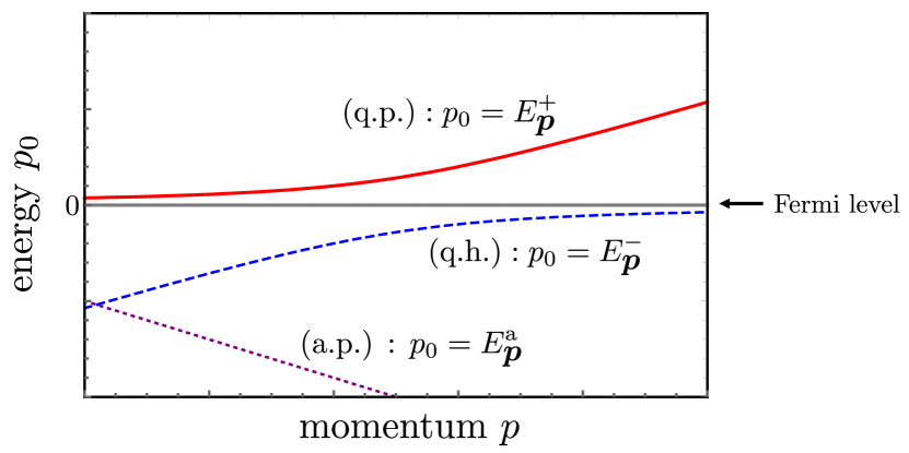
Figure 1: A schematic behavior of the dispersions in Eq. (13) ($p=|{\bm{p}}|$). Solid red, dashed blue, and dotted purple curves correspond to $p_{0}=E_{\bm{p}}^{+}$ (q.p.), $p_{0}=E_{\bm{p}}^{-}$ (q.h.), and $p_{0}=E_{\bm{p}}^{\rm a}$ (a.p.), respectively. The gray horizontal line indicates $p_{0}=0$ corresponding to the Fermi level.

Equation (12) is the Green’s function found in the previous works Yasui et al. (2019, 2017). In the present paper, we rewrite Eq. (12) into a more convenient form which shows its physical meaning manifestly. Namely, we transform Eq. (12) into the following form:

$$\tilde{\cal G}_{0}(p_{0},{\bm{p}})=\left(\begin{array}[]{cc}\tilde{\cal G}_{0}^{\bar{\psi}\psi}(p_{0},{\bm{p}})&\tilde{\cal G}_{0}^{\bar{\psi}\Psi_{v}}(p_{0},{\bm{p}})\\ \tilde{\cal G}_{0}^{{\Psi}_{v}^{\dagger}\psi}(p_{0},{\bm{p}})&\tilde{\cal G}_{0}^{{\Psi}_{v}^{\dagger}\Psi_{v}}(p_{0},{\bm{p}})\\ \end{array}\right)\ ,$$ (16)

where the elements are given as

$$\tilde{\cal G}_{0}^{\bar{\psi}\psi}(p_{0},{\bm{p}}) = i\left[\frac{U_{+}({\bm{p}})}{p_{0}-E_{\bm{p}}^{+}}+\frac{U_{-}({\bm{p}})}{p_{0}-E_{\bm{p}}^{-}}\right]\Lambda_{\rm p}$$

$$+i\frac{U_{\rm a}({\bm{p}})}{p_{0}-{E}_{\bm{p}}^{\rm a}}\Lambda_{\rm a}\,,$$

$$\tilde{\cal G}_{0}^{\bar{\psi}\Psi_{v}}(p_{0},{\bm{p}}) = i\left[\frac{V^{*}_{+}({\bm{p}})}{p_{0}-E_{\bm{p}}^{+}}+\frac{V^{*}_{-}({\bm{p}})}{p_{0}-E_{\bm{p}}^{-}}\right]\Lambda_{{\rm p}{\rm H}}\ ,$$

$$\tilde{\cal G}_{0}^{{\Psi}_{v}^{\dagger}\psi}(p_{0},{\bm{p}}) = i\left[\frac{V_{+}({\bm{p}})}{p_{0}-E_{\bm{p}}^{+}}+\frac{V_{-}({\bm{p}})}{p_{0}-E_{\bm{p}}^{-}}\right]\Lambda_{{\rm H}{\rm p}}\ ,$$

$$\tilde{\cal G}_{0}^{{\Psi}_{v}^{\dagger}\Psi_{v}}(p_{0},{\bm{p}}) = i\left[\frac{W_{+}({\bm{p}})}{p_{0}-E_{\bm{p}}^{+}}+\frac{W_{-}({\bm{p}})}{p_{0}-E_{\bm{p}}^{-}}\right]{\bm{1}}\ .$$ (17)

In these expressions, $\tilde{\cal G}_{0}^{\bar{\psi}\psi}$, $\tilde{\cal G}_{0}^{\bar{\psi}\Psi_{v}}$, $\tilde{\cal G}_{0}^{{\Psi}_{v}^{\dagger}\psi}$, and $\tilde{\cal G}_{0}^{{\Psi}_{v}^{\dagger}\Psi_{v}}$ are $4\times 4$, $4\times 2$, $2\times 4$, and $2\times 2$ matrices, respectively. Also,

$$\Lambda_{\rm p}\equiv\frac{1+\hat{\bm{p}}\cdot{\bm{\alpha}}}{2}\gamma_{0}\ ,\ \ \Lambda_{\rm a}\equiv\frac{1-\hat{\bm{p}}\cdot{\bm{\alpha}}}{2}\gamma_{0}$$ (18)

(${\bm{\alpha}}=\gamma_{0}{\bm{\gamma}}$) are the projection operators for positive- and negative-energy states of the light quark, respectively. Similarly

$$\Lambda_{{\rm p}{\rm H}}\equiv\left(\begin{array}[]{c}1\\ \hat{\bm{p}}\cdot{\bm{\sigma}}\\ \end{array}\right)\ ,\ \ \Lambda_{{\rm H}{\rm p}}\equiv\left(\begin{array}[]{cc}1&-\hat{\bm{p}}\cdot{\bm{\sigma}}\\ \end{array}\right)$$ (22)

are the operators mixing positive-energy states of the light quark and the heavy quark. ${\bm{1}}$ is a $2\times 2$ unit matrix. The weight factors $U({\bm{p}})$’s, $V({\bm{p}})$’s, and $W({\bm{p}})$’s in Eq. (17) are

$$U_{+}({\bm{p}})=\frac{2(|\Delta|^{2}+|{\bm{p}}|E_{\bm{p}}^{+})}{(E_{\bm{p}}^{-}-E_{\bm{p}}^{+})(E_{\bm{p}}^{\rm a}-E_{\bm{p}}^{+})}\ ,$$

$$U_{-}({\bm{p}})=\frac{2(|\Delta|^{2}+|{\bm{p}}|E_{\bm{p}}^{-})}{(E_{\bm{p}}^{+}-E_{\bm{p}}^{-})(E_{\bm{p}}^{\rm a}-E_{\bm{p}}^{-})}\ ,$$

$$U_{\rm a}({\bm{p}})=1\ ,$$

$$V_{+}({\bm{p}})=\frac{\Delta}{E_{\bm{p}}^{-}-E_{\bm{p}}^{+}}\ ,\ \ V_{-}({\bm{p}})=\frac{\Delta}{E_{\bm{p}}^{+}-E_{\bm{p}}^{-}}\ ,$$

$$W_{+}({\bm{p}})=\frac{E_{\bm{p}}^{+}-|{\bm{p}}|+\mu}{E_{\bm{p}}^{+}-E_{\bm{p}}^{-}}\ ,\ \ W_{-}({\bm{p}})=\frac{E_{\bm{p}}^{-}-|{\bm{p}}|+\mu}{E_{\bm{p}}^{-}-E_{\bm{p}}^{+}}\ .$$

(28)

Equations (17) and (28) clearly show that only positive-energy components of the light quark correlate with the heavy quark. Namely $U_{\rm a}({\bm{p}})$ in Eq. (28) is not changed from unity. In what follows we assume $\Delta$ to be real.

III Analysis

III.1 Linear response theory

In Sec. II we introduced an effective Lagrangian with an appropriate ansatz describing the Kondo condensate, and derived the Green’s function of fermions. Here, we show our strategy to investigate the CSE in the presence of Kondo condensate based on them. In the following calculation, we set $A_{0}=0$ since the magnetic field is not generated by $A_{0}$.

The axial current is defined by $j_{5}^{i}=\bar{\psi}\gamma^{i}\gamma_{5}\psi$ ($i=1,2,3$) including only the light-quark degrees of freedom. Its expectation value can be given by

$$\langle j_{5}^{i}(t,{\bm{x}})\rangle_{\beta}=\frac{1}{\Omega}\lim_{q_{0},{\bm{q}}\to 0}\langle\tilde{j}_{5}^{i}(q_{0},{\bm{q}})\rangle_{\beta}\ ,$$ (29)

where $\langle\cdots\rangle_{\beta}$ stands for a thermodynamic expectation value and $\Omega=\beta V$ ($\beta=1/T$ is the inverse of temperature, and $V$ is the three-dimensional volume), and $\tilde{j}_{5}^{i}(q_{0},{\bm{q}})$ is the Fourier transformation of $j_{5}^{i}(t,{\bm{x}})$. Thus, first we need to evaluate the expectation value of axial current in momentum space. In the present study, we are particularly interested in quark matter under a magnetic field with magnitude smaller than that of the Fermi energy: $\sqrt{eB}\ll\mu$. Therefore we can evaluate the CSE within the framework of the linear response theory Kapusta and Gale (2011). The linear response theory tells us that the response function to an external field takes the form of the retarded one. The retarded function could be given by an analytic continuation of the one computed within the imaginary-time formalism. Thus $\langle\tilde{j}_{5}^{i}(q_{0},{\bm{q}})\rangle_{\beta}$ in the right-hand side (RHS) of Eq. (29) is provided by

$$\langle\tilde{j}_{5}^{i}(q_{0},{\bm{q}})\rangle_{\beta}=\langle\tilde{j}_{5}^{i}(i\bar{\omega}_{n},{\bm{q}})\rangle_{\beta}|_{i\bar{\omega}_{n}\to q_{0}+i\eta}\ ,$$ (30)

with $\eta$ an infinitesimal positive number, in which $\langle\tilde{j}_{5}^{i}(i\bar{\omega}_{n},{\bm{q}})\rangle_{\beta}$ is given by

$$\langle\tilde{j}_{5}^{i}(i\bar{\omega}_{n},{\bm{q}})\rangle_{\beta}$$ (31)

$$\approx eN_{c}T\sum_{m}\int\frac{d^{3}p}{(2\pi)^{3}}{\rm tr}\Big{[}\Gamma^{i}\Gamma_{5}\tilde{\cal G}_{0}(i{\omega}_{m}+i\bar{\omega}_{n},{\bm{p}}+{\bm{q}})$$

$$\times\tilde{A}^{j}(i\bar{\omega}_{n},{\bm{q}})\Gamma^{j}\tilde{\cal G}_{0}(i{\omega}_{m},{\bm{p}})\Big{]}\ .$$

Here $6\times 6$ gamma matrices $\Gamma^{i}$ and $\Gamma_{5}$ are defined by

$$\Gamma^{i}=\left(\begin{array}[]{cc}\gamma^{i}&0\\ 0&0\\ \end{array}\right)=\left(\begin{array}[]{ccc}0&\sigma^{i}&0\\ -\sigma^{i}&0&0\\ 0&0&0\\ \end{array}\right)\ ,$$ (37)

$$\Gamma_{5}=\left(\begin{array}[]{cc}\gamma_{5}&0\\ 0&0\\ \end{array}\right)=\left(\begin{array}[]{ccc}0&1&0\\ 1&0&0\\ 0&0&0\\ \end{array}\right)\ ,$$ (43)

respectively, which act on only light quark components. Note that $\bar{\omega}_{n}=2\pi n/\beta$ is the Matsubara frequency for bosons which shows the periodic boundary condition for the imaginary-time direction, while ${\omega}_{n}=(2n+1)\pi/\beta$ is for fermions which shows the anti-periodic boundary condition. $N_{c}$ is the number of colors, and we set $N_{c}=3$ throughout this paper. $\tilde{\cal G}_{0}(i{\omega}_{m},{\bm{p}})$ in Eq. (31) can be obtained by simply replacing $p_{0}$ as $p_{0}\to i{\omega}_{m}$ in Eq. (16).

Before moving on to the detailed calculation of Eq. (31), we mention the zero-momentum limit in Eq. (29). In medium, due to the lack of Lorentz invariance, it is possible to take the following two types of zero momentum limits:

• static limit:          $\langle j_{5}^{i}\rangle^{\rm sta}_{\beta}\equiv\frac{1}{\Omega}\lim_{{\bm{q}}\to 0}\langle\tilde{j}_{5}^{i}(0,{\bm{q}})\rangle_{\beta}$ ,

• dynamical limit:  $\langle j_{5}^{i}\rangle^{\rm dyn}_{\beta}\equiv\frac{1}{\Omega}\lim_{q_{0}\to 0}\langle\tilde{j}_{5}^{i}(q_{0},{\bm{0}})\rangle_{\beta}$ .

The static limit (dynamical limit) describes the response to a magnetic field whose time dependence is slower (faster) than the equilibration of the spatial part of the system. These two limits yield different results in general Kharzeev and Warringa (2009); Hou et al. (2011); Son and Yamamoto (2013); Landsteiner et al. (2014); Kharzeev et al. (2017). Therefore in the following analysis, we will investigate the CSE in both the limits.

III.2 Calculation of $\langle\tilde{j}_{5}^{i}(i\bar{\omega}_{n},$$q$$)\rangle_{\beta}$

In Sec. III.1, we showed our strategy to evaluate the axial current $\langle j_{5}^{i}(t,{\bm{x}})\rangle_{\beta}$ within the framework of the linear response theory and presented a rather general expression of the axial current $\langle\tilde{j}_{5}^{i}(i\bar{\omega}_{n},{\bm{q}})\rangle_{\beta}$ in momentum space in Eq. (31) in the imaginary-time formalism. In this subsection, we further proceed the analytical evaluation of $\langle\tilde{j}_{5}^{i}(i\bar{\omega}_{n},{\bm{q}})\rangle_{\beta}$.

By inserting Eq. (16) into Eq. (31), the trace with respect to the Dirac indices in Eq. (43) is reduced to the one for the light quark as

$$\langle\tilde{j}_{5}^{i}(i\bar{\omega}_{n},{\bm{q}})\rangle_{\beta} = eN_{c}T\sum_{m}\int\frac{d^{3}p}{(2\pi)^{3}}{\rm tr}\Big{[}\gamma^{i}\gamma_{5}\tilde{\cal G}^{\bar{\psi}\psi}_{0}(i{\omega}_{m}^{\prime},{\bm{p}}^{\prime})$$ (44)

$$\times\tilde{A}^{j}(i\bar{\omega}_{n},{\bm{q}})\gamma^{j}\tilde{\cal G}^{\bar{\psi}\psi}_{0}(i{\omega}_{m},{\bm{p}})\Big{]}$$

(${\bm{p}}^{\prime}={\bm{p}}+{\bm{q}}$ and $i{\omega}_{m}^{\prime}=i{\omega}_{m}+i\bar{\omega}_{n}$). This reduction could be done because the axial current is defined with respect to only the light-quark degrees of freedom, and the magnetic field only couples with them now. Recalling the first line in Eq. (17), the trace calculation is straightforwardly carried out, which yields

$$\langle\tilde{j}_{5}^{i}(i\bar{\omega}_{n},{\bm{q}})\rangle_{\beta}$$

$$= -ieN_{c}\epsilon^{ijk}\tilde{A}^{k}(i\bar{\omega}_{n},{\bm{q}})T\sum_{m}\int\frac{d^{3}p}{(2\pi)^{3}}$$

$$\sum_{\zeta,\zeta^{\prime}=+,-,{\rm a}}(\epsilon_{\zeta^{\prime}}\hat{p}^{\prime j}-\epsilon_{\zeta}\hat{p}^{j})\frac{U_{\zeta^{\prime}}({\bm{p}}^{\prime})U_{\zeta}({\bm{p}})}{(i{\omega}_{m}^{\prime}-E_{{\bm{p}}^{\prime}}^{\zeta^{\prime}})(i{\omega}_{m}-E_{\bm{p}}^{\zeta})}\ .$$

In Eq. (LABEL:J5Zeta), the “sign function” $\epsilon_{\zeta}$ is defined by

$$\epsilon_{+}=\epsilon_{-}=+1\ ,$$ (46)

while

$$\epsilon_{\rm a}=-1\ ,$$ (47)

with the subscripts “$+$”, “$-$”, and “a” corresponding to the ones in Eq. (13). In deriving Eq. (LABEL:J5Zeta), we have used an identity

$${\rm tr}[\gamma^{i}\gamma_{5}\Lambda^{\prime}_{\xi^{\prime}}\gamma_{0}\gamma^{j}\Lambda_{\xi}\gamma_{0}]=-i\epsilon^{ijk}(\epsilon_{\xi^{\prime}}\hat{p}^{\prime k}-\epsilon_{\xi}\hat{p}^{k})\ ,$$ (48)

with the help of the formula ${\rm tr}[\gamma_{5}\gamma^{0}\gamma^{i}\gamma^{j}\gamma^{k}]=-4i\epsilon^{ijk}$, where $\xi,\xi^{\prime}={\rm p},{\rm a}$. In Eq. (48), the “sign function” is

$$\epsilon_{\rm p}=+1\ ,\epsilon_{\rm a}=-1\ ,$$ (49)

with the subscripts “p” and “a” corresponding to the ones in Eq. (18).

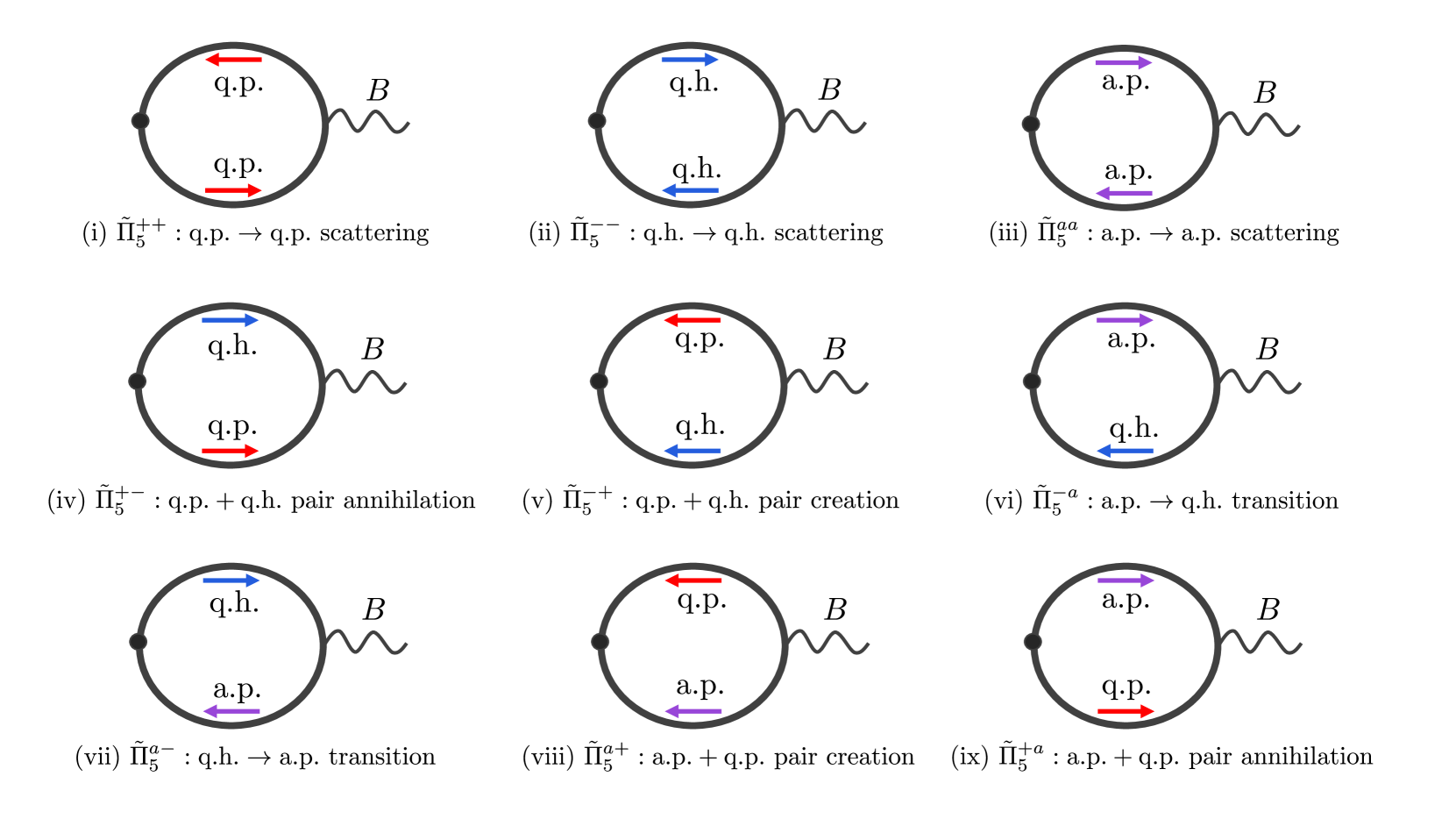
Figure 2: Diagrammatic interpretation of each term in Eq. (57). The arrows are put such that the corresponding modes carry their positive energies.

Equation (LABEL:J5Zeta) includes an infinite sum with respect to the Matsubara frequency. This summation can be done by transforming the infinite series into a contour integral in the complex plane. Namely, we make use of the Abel-Plana formula Kapusta and Gale (2011)

$$T\sum_{m}F(p_{0}=i{\omega}_{m})$$ (50)

$$= \frac{1}{2\pi i}\int_{-i\infty}^{i\infty}dp_{0}\frac{1}{2}\Big{[}F(p_{0})+F(-p_{0})\Big{]}$$

$$-\frac{1}{2\pi i}\int_{-i\infty+\eta}^{i\infty+\eta}dp_{0}\Big{[}F(p_{0})+F(-p_{0})\Big{]}f_{F}(p_{0})\ ,$$

where $F(p_{0})$ is an arbitrary function which is analytic on the imaginary axis, and $f_{F}(p_{0})=\frac{1}{{\rm e}^{\beta p_{0}}+1}$ is the Fermi-Dirac distribution function. The calculation can be carried out without difficulty by means of the Cauchy’s residue theorem, yielding

$$\langle\tilde{j}_{5}^{i}(i\bar{\omega}_{n},{\bm{q}})\rangle_{\beta}=ie\epsilon^{ijk}\tilde{A}^{k}(i\bar{\omega}_{n},{\bm{q}})\tilde{\Pi}_{5}^{j}(i\bar{\omega}_{n},{\bm{q}})\ ,$$ (51)

in which we have defined

$$\tilde{\Pi}_{5}^{j}(i\bar{\omega}_{n},{\bm{q}})\equiv-N_{c}\int\frac{d^{3}p}{(2\pi)^{3}}\sum_{\zeta,\zeta^{\prime}={+},{-},{\rm a}}(\epsilon_{\zeta^{\prime}}\hat{p}^{\prime j}-\epsilon_{\zeta}\hat{p}^{j})\frac{U_{\zeta^{\prime}}({\bm{p}}^{\prime})U_{\zeta}({\bm{p}})}{i\bar{\omega}_{n}-E_{{\bm{p}}^{\prime}}^{\zeta^{\prime}}+E_{\bm{p}}^{\zeta}}\left[f_{F}(E_{\bm{p}}^{\zeta})-f_{F}(E_{{\bm{p}}^{\prime}}^{\zeta^{\prime}})\right]\ .$$ (52)

In Eq. (51), $\tilde{\Pi}_{5}^{j}(i\bar{\omega}_{n},{\bm{q}})$ must be proportional to $q^{j}$ due to its Lorentz structure. Thus, by defining $\tilde{\Pi}_{5}(i\bar{\omega}_{n},{\bm{q}})$ in terms of

$$\tilde{\Pi}_{5}^{j}(i\bar{\omega}_{n},{\bm{q}})\equiv\tilde{\Pi}_{5}(i\bar{\omega}_{n},{\bm{q}})q^{j}\ ,$$ (53)

now Eq. (51) reads

$$\langle\tilde{j}_{5}^{i}(i\bar{\omega}_{n},{\bm{q}})\rangle_{\beta} = ie\epsilon^{ijk}q^{j}\tilde{A}^{k}(i\bar{\omega}_{n},{\bm{q}})\tilde{\Pi}_{5}(i\bar{\omega}_{n},{\bm{q}})$$ (54)

$$= e\tilde{B}(i\bar{\omega}_{n},{\bm{q}})\tilde{\Pi}_{5}(i\bar{\omega}_{n},{\bm{q}})\ .$$

In the second line of Eq. (54), we have made use of $\tilde{B}^{i}(i\bar{\omega}_{n},{\bm{q}})=i\epsilon^{ijk}q^{j}\tilde{A}^{k}(i\bar{\omega}_{n},{\bm{q}})$ [$\tilde{B}^{i}(q_{0},{\bm{q}})$ is defined by the Fourier transformation of $B^{i}(t,{\bm{x}})$]. We note that $\tilde{\Pi}_{5}(i\bar{\omega}_{n},{\bm{q}})$ can be “solved” as

$$\tilde{\Pi}_{5}(i\bar{\omega}_{n},{\bm{q}})=\frac{1}{|{\bm{q}}|^{2}}\tilde{\Pi}_{5}^{j}(i\bar{\omega}_{n},{\bm{q}})q^{j}$$ (55)

from Eq. (53).

Equation (54) shows that $\tilde{\Pi}_{5}(i\bar{\omega}_{n},{\bm{q}})$ is the response function of axial current to a magnetic field. Concretely, from Eqs. (52) and (55), the response function is expressed as

$$\tilde{\Pi}_{5}(i\bar{\omega}_{n},{\bm{q}})=\sum_{\zeta,\zeta^{\prime}=+,-,{\rm a}}\tilde{\Pi}^{\zeta^{\prime}\zeta}_{5}(i\bar{\omega}_{n},{\bm{q}})$$ (56)

with

$$\tilde{\Pi}^{\zeta^{\prime}\zeta}_{5}(i\bar{\omega}_{n},{\bm{q}})\equiv-\frac{N_{c}}{|{\bm{q}}|^{2}}\int\frac{d^{3}p}{(2\pi)^{3}}\Big{[}\epsilon_{\zeta^{\prime}}(\hat{\bm{p}}^{\prime}\cdot{\bm{q}})-\epsilon_{\zeta}(\hat{\bm{p}}\cdot{\bm{q}})\Big{]}\frac{U_{\zeta^{\prime}}({\bm{p}}^{\prime})U_{\zeta}({\bm{p}})}{i\bar{\omega}_{n}-E_{{\bm{p}}^{\prime}}^{\zeta^{\prime}}+E_{\bm{p}}^{\zeta}}\left(f_{F}(E_{\bm{p}}^{\zeta})-f_{F}(E_{{\bm{p}}^{\prime}}^{\zeta^{\prime}})\right)\ .$$ (57)

After performing the analytic continuation to the real-time formalism and taking zero limit of the external momentum ($q_{0},{\bm{q}}$) properly, static and dynamical limits for $\langle j_{5}^{i}\rangle_{\beta}$ can be evaluated from Eq. (54) as

$$\langle j_{5}^{i}(t,{\bm{x}})\rangle_{\beta}^{\rm sta}=eB\tilde{\Pi}_{5}^{\rm sta},$$

$$\langle j_{5}^{i}(t,{\bm{x}})\rangle_{\beta}^{\rm dyn}=eB\tilde{\Pi}_{5}^{\rm dyn}\ ,$$ (58)

respectively from Eqs. (29) and (30), with the definitions of

$$\tilde{\Pi}_{5}^{\rm sta}\equiv\lim_{{\bm{q}}\to{\bm{0}}}\tilde{\Pi}_{5}(0,{\bm{q}})\ ,$$

$$\tilde{\Pi}_{5}^{\rm dyn}\equiv\lim_{q_{0}\to 0}\tilde{\Pi}_{5}(q_{0},{\bm{0}})\ .$$ (59)

We also used $\tilde{B}(q_{0}=0,{\bm{q}}={\bm{0}})=\Omega B$. By carrying out the angular integral in Eq. (56) in two limits, the response function can be analytically obtained apart from the $|{\bm{p}}|$ integral. We note that a rather detailed discussion on the response function in static and dynamical limits is given in Appendix B.

At the end of this subsection, we explain the details of the nine contributions in Eq. (57) obtained by setting $\zeta,\zeta^{\prime}=+,-,{\rm a}$. Diagrammatically, these contributions can be understood as in Fig. 2. In this figure, the arrows are put in such a way that the corresponding modes carry their positive energies. We note that the momentum integrals of the loops in Fig. 2 do not include any ultraviolet divergences. According to Eqs. (187) and (188) in Appendix B, each contribution in Eq. (57) in static limit and dynamical limit after the analytic continuation is found to satisfy

$$\lim_{{\bm{q}}\to{\bm{0}}}\tilde{\Pi}_{5}^{\zeta\zeta}(0,{\bm{q}}) = -N_{c}\int\frac{d^{3}p}{(2\pi)^{3}}{\cal I}_{\zeta}({\bm{p}})\frac{\partial f_{F}(E_{\bm{p}}^{\zeta})}{\partial|{\bm{p}}|}\ ,$$

$$\lim_{q_{0}\to 0}\tilde{\Pi}_{5}^{\zeta\zeta}(q_{0},{\bm{0}}) = 0\ ,$$ (60)

[${\cal I}_{\zeta}({\bm{p}})$ is a function of ${\bm{p}}$ ] for $\tilde{\Pi}_{5}^{++}$, $\tilde{\Pi}_{5}^{--}$ and $\tilde{\Pi}_{5}^{\rm{aa}}$, while

$$\lim_{{\bm{q}}\to{\bm{0}}}\tilde{\Pi}_{5}^{\zeta^{\prime}\zeta}(0,{\bm{q}})=\lim_{q_{0}\to 0}\tilde{\Pi}_{5}^{\zeta^{\prime}\zeta}(q_{0},{\bm{0}})$$ (61)

for the remaining ones $(\zeta\neq\zeta^{\prime})$. In other words, only the diagrams of (i), (ii), and (iii) in Fig. 2, which correspond to the scattering processes of the identical particle by the magnetic field: ${\rm q.p.}\to{\rm q.p.}$, ${\rm q.h.}\to{\rm q.h.}$, and ${\rm a.p.}\to{\rm a.p.}$ (or intraband scattering processes in the terminology of condensed matter physics), can generate the difference between the results in static limit and dynamical limit. Such a difference between the static and dynamical limits was also found in Ref. Araki et al. (2020). In this reference, we investigated the spin-orbital crossed susceptibility, namely the response of spin polarization to a magnetic field, in which a relativistic (linear) band and a nonrelativistic band coexist.

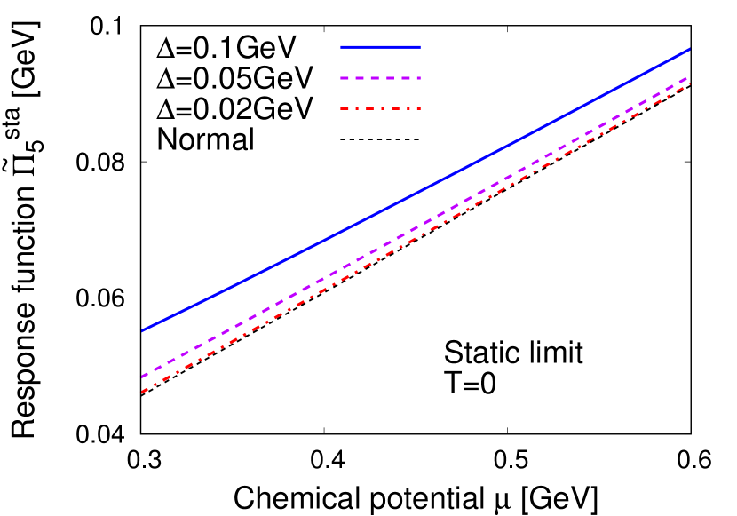
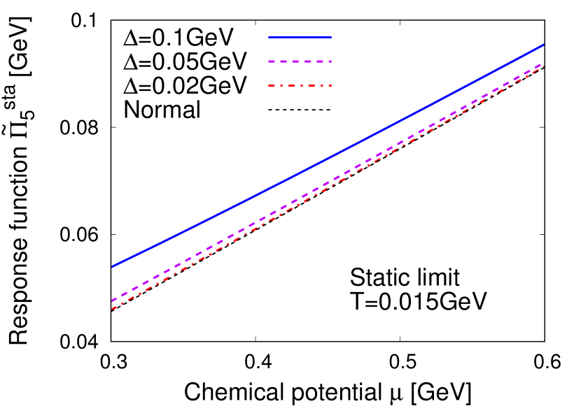
Figure 3: The $\mu$ dependence of response function in static limit ($\tilde{\Pi}_{5}^{\rm sta}$) with $\Delta=0.02$ GeV (red dashed-dotted), $\Delta=0.05$ GeV (purple dashed), and $\Delta=0.1$ GeV (blue solid). The black dashed curve indicates the response function in the normal matter given in Eq. (62).

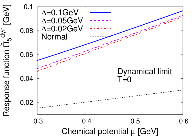
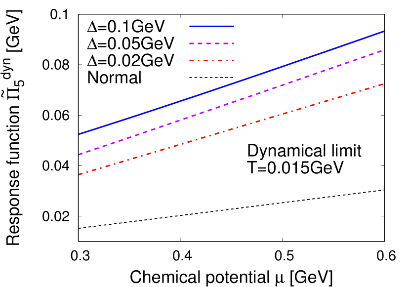
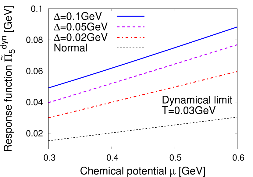
Figure 4: The $\mu$ dependence of response function in dynamical limit ($\tilde{\Pi}_{5}^{\rm dyn}$) with $\Delta=0.02$ GeV (red dashed-dotted), $\Delta=0.05$ GeV (purple dashed), and $\Delta=0.1$ GeV (blue solid). The black dashed curve indicates the response function in the normal matter given in Eq. (63).

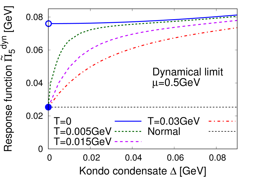
Figure 5: The gap dependence of response function in static limit ($\tilde{\Pi}_{5}^{\rm sta}$) (upper panel) and in dynamical limit ($\tilde{\Pi}_{5}^{\rm dyn}$) (lower panel) at $\mu=0.5$ GeV and at several temperatures. The black dashed line indicates the response function in the normal matter given in Eq. (62). Blue filled or open circle in dynamical limit mean the discontinuous behavior at $T=0$ (see the main text).

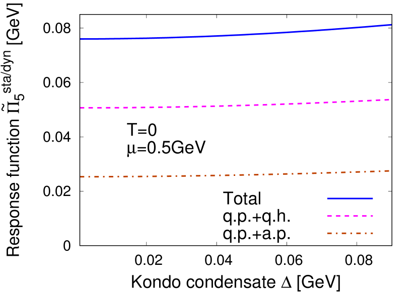
Figure 6: The $\mu$ dependence at $T=0$ and $\Delta=0.1$ GeV of each process contributing to the response function (upper panel), and the $\Delta$ dependence at $T=0$ and $\mu=0.5$ GeV of them (lower panel). We compare the total value of response function (blue solid), the sum of pair creation and pair annihilation processes of ${\rm q.p.}+{\rm q.h.}$ (magenta dashed), and the sum of pair creation and pair annihilation processes of ${\rm q.p.}+{\rm a.p.}$ (brown dashed-dotted).

IV Numerical results

In Sec. III we showed the detailed procedure to compute the axial current induced by a magnetic field in the presence of Kondo condensate in static and dynamical limits. In this section, we present numerical results of Eq. (59) and examine the impact of Kondo effect on CSE. For the sake of clarity, here we do not solve the gap equation to determine the magnitude, and its density dependence of $\Delta$ and simply regard it as a constant parameter.

IV.1 Density dependence of the CSE

First, we show the density dependence of the response function of CSE obtained in the present work.

In Fig. 3 and Fig 4, the $\mu$ dependences of response function $\tilde{\Pi}_{5}^{\rm sta}$ in static limit and $\tilde{\Pi}_{5}^{\rm dyn}$ in dynamical limit with $\Delta=0.02$ GeV (red), $\Delta=0.05$ GeV (purple), and $\Delta=0.1$ GeV (blue) are plotted, respectively. The black dashed line indicates the response function in the normal matter ($\Delta=0$), i.e.,

$$\tilde{\Pi}^{\rm sta}_{5}|_{\Delta=0} = \frac{N_{c}}{2\pi^{2}}\mu\ ,$$ (62)

$$\tilde{\Pi}^{\rm dyn}_{5}|_{\Delta=0} = \frac{N_{c}}{6\pi^{2}}\mu\ ,$$ (63)

at any temperatures. We have put this line so as to compare the results with and without Kondo effect more clearly. We have shown the results in the range of $0.3\,{\rm GeV}<\mu<0.6\,{\rm GeV}$ in which the Kondo condensate is expected to appear significantly within reasonable model parameters, as suggested by the previous works Yasui et al. (2019, 2017).

Figures 3 and 4 show that the Kondo effect enhances the CSE in both static limit and dynamical limit. In particular, the response function in dynamical limit can be enhanced by a factor of approximately three. Besides, those figures show that the results in static limit and dynamical limit at $T=0$ coincide with each other: $\tilde{\Pi}^{\rm sta}_{5}=\tilde{\Pi}^{\rm dyn}_{5}$. Note that the magnitude of $\Delta$ was found to be $\Delta\approx 0.085$ GeV at $\mu=0.5$ GeV in the previous work based on the NJL-type analysis Yasui et al. (2019, 2017). Therefore, we can conclude that the influence of Kondo effect on CSE with a reasonable value of $\Delta$ is significantly large, showing that the heavy impurities in quark matter is expected to play an important role in the transport phenomena induced by a magnetic field. The large enhancement of the response function in dynamical limit is consistent with the finding in Ref. Araki et al. (2020).

IV.2 $\Delta$ dependence of the CSE

Next, we study the $\Delta$ dependence of the CSE to examine the influence of Kondo condensate $\Delta$ on the CSE in more detail.

In Fig. 5 we display the $\Delta$ dependence of the response function in static limit (upper panel) and dynamical limit (lower panel) at $\mu=0.5$ GeV and at several temperatures. The black dashed line indicates the response function in the normal matter given in Eq. (62). The lower panel tells us that, $\tilde{\Pi}_{5}^{\rm dyn}$ for small $\Delta$ with $\Delta\neq 0$ is enhanced largely due to an effect generated by the Kondo condensate, although it converges on the result of normal matter in dynamical limit provided in Eq. (63) at $\Delta=0$. Such a sudden and large enhancement around $\Delta=0$ stems from the fact that the effect of $\Delta$ is nonperturbative around the Fermi level, which can be understood as follows. The CSE is mostly generated by the response of fermions in the vicinity of the Fermi level ($|{\bm{p}}|\approx\mu$) in the momentum integrals of the loops. However, the factor of $\sqrt{(|{\bm{p}}|-\mu)^{2}+8\Delta^{2}}$ appearing in $E_{\bm{p}}^{\pm}$ prohibits us from expanding $E_{\bm{p}}^{\pm}$ with respect to $\Delta$ around $|{\bm{p}}|=\mu$ now, because the magnitudes of $(|{\bm{p}}|-\mu)^{2}$ and $8\Delta^{2}$ are comparable order in this case. As a result, the Taylor expansion of the response function with respect to $\Delta$ should fail, and hence the modification of $\tilde{\Pi}_{5}^{\rm dyn}$ at small $\Delta$ is significant.

The signature of the nonperturbative effect by $\Delta$ can be seen prominently at $T=0$ in the lower panel of Fig. 5. Namely, at $T=0$, $\tilde{\Pi}_{5}^{\rm dyn}$ at $\Delta\neq 0$ varies continuously, but only at $\Delta=0$ it jumps to the result of normal matter in dynamical limit discontinuously. Here, we provide some mathematical explanations for the origin of the discontinuity. As shown in Eqs. (60) and (61), the difference between the results in static and dynamical limits originates from the scattering process of the identical particles, i.e., from the diagrams (i), (ii), and (iii) in Fig. 2. Below we focus on the diagram (i). At zero temperature, from Eq. (60), the response functions from the diagram (i) in static and dynamical limits are of the forms

$$\lim_{{\bm{q}}\to{\bm{0}}}\tilde{\Pi}_{5}^{++}(0,{\bm{q}})\overset{T=0}{=}-N_{c}\int\frac{d^{3}p}{(2\pi)^{3}}{\cal I}_{+}({\bm{p}})\frac{E_{\bm{p}}^{+}}{E_{\bm{p}}^{+}-E_{\bm{p}}^{-}}\delta(E_{\bm{p}}^{+})\ ,$$

$$\lim_{q_{0}\to 0}\tilde{\Pi}_{5}^{++}(q_{0},{\bm{0}})\overset{T=0}{=}0\ ,$$ (64)

respectively. These results coincide with each other, even when $\Delta$ is infinitesimally small, since $E_{\bm{p}}^{+}$ and $E_{\bm{p}}^{+}-E_{\bm{p}}^{-}$ are always positive in this case, resulting in

$$\lim_{{\bm{q}}\to{\bm{0}}}\tilde{\Pi}_{5}^{++}(0,{\bm{q}})\overset{T=0}{=}0\ .$$ (65)

Hence, $\tilde{\Pi}^{\rm sta}_{5}=\tilde{\Pi}^{\rm dyn}_{5}$ holds for $\Delta\neq 0$. On the other hand, when $\Delta$ is exactly zero, the upper equation of Eq. (64) is no longer zero because $E_{\bm{p}}^{+}|_{\Delta=0}=\theta(|{\bm{p}}|-\mu)(|{\bm{p}}|-\mu)$ and $E_{\bm{p}}^{-}|_{\Delta=0}=\theta(\mu-|{\bm{p}}|)(|{\bm{p}}|-\mu)$ can reach zero, yielding $\tilde{\Pi}^{\rm sta}_{5}\neq\tilde{\Pi}^{\rm dyn}_{5}$. As a result, the discontinuous behavior of the blue curve of lower panel in Fig. 5 at $\Delta\to 0$ emerges. The similar explanation can be also applied to (ii) and (iii). The discontinuity at $\Delta=0$, however, should not be taken too seriously, because in realistic measurements, this discontinuity would be smeared by the finite relaxation time.

In association with the sudden and large enhancement at $T\neq 0$ (and the discontinuity at $T=0$) in dynamical limit, in Ref. Satow and Yee (2014), it was found that, in the normal matter the damping rate of free quark enhances the CSE in dynamical limit to coincide with the one in static limit. Thus, by focusing on the fact that nonzero $\Delta$ causes the sudden and large enhancement of the response function in dynamical limit resulting in the similar behavior to static limit, as shown in Fig. 5, we speculate that there would be an analogy between the inclusion of damping rate in the normal matter and the presence of Kondo condensate $\Delta$. A detailed comparison between the present analysis and the one in Ref. Satow and Yee (2014) is left for future study.

IV.3 Separate contributions to the CSE

Finally, we give a physical interpretation of how the each diagram in Fig. 2 contributes to the response function.

Again for the sake of clarity, we restrict ourselves to vanishing temperature. At $T=0$, the Pauli principle forces the intermediate states of the loops to excite above the Fermi level, i.e., at least one of the modes inside the loop must be ${\rm q.p.}$ because only this mode lies above the Fermi level as shown in Fig. 1. In fact we can confirm that only the diagrams (iv) and (v) for ${\rm q.p.}+{\rm q.h.}$ and (viii) and (ix) for ${\rm q.p.}+{\rm a.p.}$ in Fig. 2 contribute to the CSE through the pair creation and pair annihilation processes. We note that the contribution from the diagram (i) vanishes at zero temperature as explained around Eqs. (64) and (65) in detail.

In Fig. 6 we show the $\mu$ dependence of each process contributing to the response function at $T=0$ and $\Delta=0.1$ GeV (upper panel), and the $\Delta$ dependence of them at $T=0$ and $\mu=0.5$ GeV (lower panel). We note that the point for $\Delta=0$ is excluded in the lower panel to avoid the discontinuity explained in Sec. IV.2. In Fig. 6, the blue curve indicates the total value of response function, while the magenta curve corresponds to the sum of ${\rm q.p.}+{\rm q.h.}$ pair creation and pair annihilation, and the brown one corresponds to the sum of ${\rm q.p.}+{\rm a.p.}$ pair creation and pair annihilation. Only these processes contribute to the response function due to the reason stated above. Note that at zero temperature the response functions in static and dynamical limits coincide: $\tilde{\Pi}_{5}^{\rm sta}=\tilde{\Pi}_{5}^{\rm dyn}$ as found in Sec. IV.1. Figure 6 shows that the contribution from ${\rm q.p.}+{\rm q.h.}$ process and that of ${\rm q.p.}+{\rm a.p.}$ are approximately in the ratio of $2:1$ for any values of $\mu$ or $\Delta$. This ratio is easily understood because the former process includes two modes (both ${\rm q.p.}$ and ${\rm q.h.}$) lying in the vicinity of the Fermi level while the latter includes only one mode (only ${\rm q.p.}$) there.

At finite temperature, the above picture does not change significantly as long as the temperature is smaller than the chemical potential $\mu$. In fact this is the case in the present work so that the contributions from diagrams (i), (ii), (iii), (vi), and (vii) in Fig. 2 remain small.

V Gauge invariance

Here we discuss the gauge invariance in our calculations. If we assume a charged Kondo condensate with $e_{q}\neq e_{Q}$, then the condensate carries an electric charge and leads to the spontaneous breakdown of the electromagnetic $U(1)_{\rm EM}$ invariance. In this case, we have to correct the vertex for the coupling between the quarks and the magnetic field in order to recover the gauge invariance, leading to the appearance of the NG mode. This treatment is an analogue of the derivation of NG mode appearing in the theory of superconductivity Schrieffer (1999), or that of pion in chiral symmetry breaking Cheng and Li (1994). On the other hand, even when we assume the charge-neutral Kondo condensate as in the present study [recall Eq. (5)], the nontrivial structure of the hedgehog ansatz (6) still requires to correct the vertex for the gauge invariance. In actuality, such a vertex correction is found not to affect our results considerably as it will be explained later. Rigorous arguments on the gauge invariance are, however, important and useful in the study of response to the external gauge field.

The underlying theory of the effective model (8), i.e., QCD and QED, must possess the electromagnetic $U(1)_{\rm EM}$ gauge invariance. Thus the Ward-Takahashi identity together with the Dyson-Schwinger equation with respect to vector-axialvector current correlator tells us that the vertex $\Gamma^{\mu}$ between the gauge field and the quarks must obey the following identity Nambu (1960)

$$q_{\mu}\Gamma^{\mu}=-i{\cal G}^{-1}(p_{0}^{\prime},{\bm{p}}^{\prime})Q+Qi{\cal G}^{-1}(p_{0},{\bm{p}})$$ (66)

($p^{\prime}=p+q$), where $\Gamma^{\mu}$ is the $6\times 6$ vertex matrix

$$\Gamma^{\mu}\equiv\left(\begin{array}[]{cc}\Gamma^{\mu}_{A\bar{\psi}\psi}&\Gamma^{\mu}_{A\bar{\psi}\Psi_{v}}\\ \Gamma^{\mu}_{A\Psi_{v}^{\dagger}\psi}&\Gamma^{\mu}_{A\Psi_{v}^{\dagger}\Psi_{v}}\\ \end{array}\right).$$ (69)

Here, for example, the subscript of $\Gamma^{\mu}_{A\bar{\psi}\psi}$ represents the type of gauge interaction such as $A^{\mu}\bar{\psi}\psi$. $Q$ is a charge matrix

$$Q=\left(\begin{array}[]{ccc}e_{q}&0\\ 0&e_{Q}\\ \end{array}\right)\ ,$$ (72)

where we have assumed the electric charges of light and heavy quarks are not identical for a general discussion. $i{\cal G}^{-1}(p_{0},{\bm{p}})$ is the inverse of the full Green’s function in general. Within the present work, it can be read by the Lagrangian (8) [where we do not necessarily assume Eq. (7)]:

$$i{\cal G}^{-1}(p_{0},{\bm{p}})=\left(\begin{array}[]{cc}i{\cal G}_{\bar{\psi}\psi}^{-1}(p_{0},{\bm{p}})&i{\cal G}_{\bar{\psi}\Psi_{v}}^{-1}(p_{0},{\bm{p}})\\ i{\cal G}_{\Psi_{v}^{\dagger}\psi}^{-1}(p_{0},{\bm{p}})&i{\cal G}_{\Psi_{v}^{\dagger}\Psi_{v}}^{-1}(p_{0},{\bm{p}})\\ \end{array}\right)$$ (75)

with

$$i{\cal G}_{\bar{\psi}\psi}^{-1}(p_{0},{\bm{p}}) = {\ooalign{\hfil/\hfil\crcr$p$}}+\mu\gamma_{0}\ ,$$ (78)

$$i{\cal G}_{\bar{\psi}\Psi_{v}}^{-1}(p_{0},{\bm{p}}) = \Delta\left(\begin{array}[]{c}1\\ -\hat{\bm{p}}\cdot{\bm{\sigma}}\\ \end{array}\right)\ ,$$ (81)

$$i{\cal G}_{\Psi_{v}^{\dagger}\psi}^{-1}(p_{0},{\bm{p}}) = \Delta\left(\begin{array}[]{cc}1&\hat{\bm{p}}\cdot{\bm{\sigma}}\\ \end{array}\right)\ ,$$ (83)

$$i{\cal G}_{\Psi_{v}^{\dagger}\Psi_{v}}^{-1}(p_{0},{\bm{p}}) = p_{0}{\bm{1}}\ .$$ (84)

Thus, each component of the Ward-Takahashi identity in Eq. (66) reads

$$q_{\mu}\Gamma^{\mu}_{A\bar{\psi}\psi} = -e_{q}{\ooalign{\hfil/\hfil\crcr$q$}}\ ,$$ (87)

$$q_{\mu}\Gamma^{\mu}_{A\bar{\psi}\Psi_{v}} = \Delta\left(\begin{array}[]{c}e_{q}-e_{Q}\\ e_{Q}\hat{\bm{p}}^{\prime}\cdot{\bm{\sigma}}-e_{q}\hat{\bm{p}}\cdot{\bm{\sigma}}\\ \end{array}\right)\ ,$$ (90)

$$q_{\mu}\Gamma^{\mu}_{A\Psi_{v}^{\dagger}\psi} = \Delta\left(\begin{array}[]{cc}e_{Q}-e_{q}&-e_{q}\hat{\bm{p}}^{\prime}\cdot{\bm{\sigma}}+e_{Q}\hat{\bm{p}}\cdot{\bm{\sigma}}\\ \end{array}\right)\ ,$$ (92)

$$q_{\mu}\Gamma^{\mu}_{A\Psi_{v}^{\dagger}\Psi_{v}} = -e_{Q}q_{0}{\bm{1}}\ .$$ (93)

For the diagonal components, $A^{\mu}\bar{\psi}\psi$ and $A^{\mu}\Psi_{v}^{\dagger}\Psi_{v}$, we can safely use their bare vertices:

$$\Gamma^{\mu}_{A\bar{\psi}\psi}=-e_{q}\gamma^{\mu}\ ,\ \ \Gamma^{\mu}_{A\Psi_{v}^{\dagger}\Psi_{v}}=-e_{Q}\delta^{\mu 0}{\bm{1}}\ .$$ (94)

On the other hand, for the off-diagonal components, $A^{\mu}\bar{\psi}\Psi_{v}$ and $A^{\mu}\Psi_{v}^{\dagger}\psi$, we cannot use their bare vertices, and they need to be corrected in such a way that they satisfy the identities in Eq. (93).

When $e_{q}\neq e_{Q}$, the second and third identities in Eq. (93) suggest an existence of collective mode (NG mode) coupling with the vertex, because the RHS in the limit of $q_{0},{\bm{q}}\to 0$ does not vanish in this case Nambu (1960). The appearance of NG mode can be also understood by the fact that $\Delta\sim\langle\Psi_{v}^{\dagger}\psi\rangle$ with $e_{q}\neq e_{Q}$ carries its nonzero electric charge leading to the spontaneous breakdown of $U(1)_{\rm EM}$ symmetry. This collective mode (NG mode) is analogous to the one in the theory of superconductivity Schrieffer (1999).

On the other hand, when $e\equiv e_{q}=e_{Q}$ as we have assumed in the present study, the NG mode related to the spontaneous breakdown of $U(1)_{\rm EM}$ symmetry does not appear. However, modifications of the vertices are still required, as seen by the RHS of second and third identities in Eq. (93):

$$q_{\mu}\Gamma^{\mu}_{A\bar{\psi}\Psi_{v}} = e\Delta\left(\begin{array}[]{c}0\\ (\hat{\bm{p}}^{\prime}-\hat{\bm{p}})\cdot{\bm{\sigma}}\\ \end{array}\right)\ ,$$ (97)

$$q_{\mu}\Gamma^{\mu}_{A\Psi_{v}^{\dagger}\psi} = e\Delta\left(\begin{array}[]{cc}0&-(\hat{\bm{p}}^{\prime}-\hat{\bm{p}})\cdot{\bm{\sigma}}\\ \end{array}\right)\ .$$ (99)

Obviously the modifications originate from the nontrivial momentum alignment caused by hedgehog ansatz (6). Equation (99) can be solved with respect to $\Gamma^{\mu}_{A\bar{\psi}\Psi_{v}}$ and $\Gamma^{\mu}_{A\Psi_{v}^{\dagger}\psi}$ by imposing some assumptions. For example, if we restrict ourselves to the vicinity of $q^{\mu}=0$, then the Ward-Takahashi identities for $\Gamma^{\mu}_{A\bar{\psi}\Psi_{v}}$ and $\Gamma^{\mu}_{A\Psi_{v}^{\dagger}\psi}$ are solved, and we obtain

$$\Gamma^{\mu}_{A\bar{\psi}\Psi_{v}} \approx -e\Delta\delta^{i\mu}\left(\begin{array}[]{c}0\\ \frac{\sigma^{i}-(\hat{\bm{p}}\cdot{\bm{\sigma}})\hat{p}^{i}}{|{\bm{p}}|}\\ \end{array}\right)\ ,$$ (102)

$$\Gamma^{\mu}_{A\Psi_{v}^{\dagger}\psi} \approx e\Delta\delta^{i\mu}\left(\begin{array}[]{cc}0&\frac{\sigma^{i}-(\hat{\bm{p}}\cdot{\bm{\sigma}})\hat{p}^{i}}{|{\bm{p}}|}\\ \end{array}\right)\ .$$ (104)

The vertex corrections in Eq. (104) can give rise to additional contributions to the axial current as

$$\langle\delta\tilde{j}_{5}^{i}(i\bar{\omega}_{n},{\bm{q}})\rangle_{\beta}$$ (107)

$$\approx -N_{c}T\sum_{m}\int\frac{d^{3}p}{(2\pi)^{3}}{\rm tr}\Big{[}\Gamma^{i}\Gamma_{5}\tilde{\cal G}_{0}(i{\omega}_{m}+i\bar{\omega}_{n},{\bm{p}}+{\bm{q}})$$

$$\times\tilde{A}^{j}(i\bar{\omega}_{n},{\bm{q}})\left(\begin{array}[]{cc}0&\Gamma_{A\bar{\psi}\Psi_{v}}^{j}\\ \Gamma_{A\Psi_{v}^{\dagger}\psi}^{j}&0\\ \end{array}\right)\tilde{\cal G}_{0}(i{\omega}_{m},{\bm{p}})\Big{]}\,,$$

[compare to Eq. (31)]. Here, we note that the RHS of Eq. (107) is proportional to $\Delta^{2}$, because Eq. (104) is proportional to $\Delta$ and computation of the trace in Eq. (107) picks up another $\Delta$ in $V_{+}({\bm{p}})$ or $V_{-}({\bm{p}})$ in Eq. (17). Namely the additional contributions from the vertex corrections may be small in a realistic situation where $\Delta$ is always smaller than $\mu$.

The above discussion suggests that, while the method in deriving the response functions in Sec. IV seem to violate the $U(1)_{\rm EM}$ gauge invariance due to lack of the vertex corrections, such a violation is expected to be relatively small and gives only a subleading effect on our findings as long as we assume $e\equiv e_{q}=e_{Q}$. On the other hand, when we take into account the difference between the electric charges of light and heavy quarks, the effects from the vertex correction would become rather important because of the appearance of NG mode Nambu (1960). Therefore, the study of CSE in the presence of Kondo condensate with other choices of electric charges would be of interest, and we leave such an examination for future publication.

VI Conclusions

In this paper we studied the axial current induced by a magnetic field, i.e., the chiral separation effect (CSE) with the Kondo effect. To demonstrate the impact of Kondo effect on the CSE in a transparent way, we employed a simple effective Lagrangian incorporating a condensate between a light quark and a heavy quark, which is the so-called Kondo condensate.

When we evaluate the CSE by means of the linear response theory, we can define the axial current in the two types of limits: static limit and dynamical limit. The former (latter) describes an induced current under an external magnetic field whose time dependence is slower (faster) than the equilibration of the spatial part of the system, and in general they yield different results. Thus we studied the response function of the axial current to the magnetic field in those two limits. We found that the Kondo effect enhances the CSE in both the static limit and dynamical limit, and particularly the CSE in dynamical limit can be increased by a factor of approximately three in the range of the reasonable value of Kondo condensate. Those results clearly show that the Kondo effect arising from heavy impurities in quark matter, can play an important role in the transport phenomena of light quarks induced by a magnetic field.

The results obtained in this paper are expected to contribute to a better understanding of transport phenomena induced by a magnetic field in quark matter with heavy impurities. In condensed matter physics, our findings are related to the electron spin polarization (spin magnetization) in the response to a magnetic field in Dirac/Weyl semimetals having a band structure including both relativistic and nonrelativistic degrees of freedom, since the spin polarization is related to axial current by spin-momentum locking Araki et al. (2020). In particular, the response function of the CSE to a magnetic field is equivalent to the so-called spin-orbital crossed susceptibility Tserkovnyak et al. (2015); Koshino and Hizbullah (2016); Nakai and Nomura (2016); Suzuura and Ando (2016); Ando and Suzuura (2017); Ominato et al. (2019) which constitutes a part of the magnetic susceptibility, as pointed out in Ref. Araki et al. (2020).

In what follows, we give discussions related to the present study. While we investigated the CSE with Kondo effect at vanishing frequency of magnetic field in this paper, our analysis can be applied to the one at finite frequency as in Refs. Kharzeev and Warringa (2009); Yee (2009); Landsteiner et al. (2014); Satow and Yee (2014); Kharzeev et al. (2017) for the CME and in Ref. Landsteiner et al. (2014) for the CSE. Such a study will be important for a more realistic situation such as (low-energy and peripheral) heavy-ion collisions where the strength of a magnetic field produced after a nucleus-nucleus collision evolves with time.

Moreover, our analysis can be easily applied to the study of the chiral magnetic effect (CME) Kharzeev (2006); Kharzeev and Zhitnitsky (2007); Kharzeev et al. (2008); Fukushima et al. (2008) and the chiral vortical effect (CVE) Vilenkin (1979, 1980b); Erdmenger et al. (2009); Banerjee et al. (2011); Son and Surowka (2009); Landsteiner et al. (2011); Stephanov and Yin (2012); Abramchuk et al. (2018) with the Kondo effect. The CME describes the vector current induced by a magnetic field in chirality imbalanced matter Kharzeev (2006); Kharzeev and Zhitnitsky (2007); Kharzeev et al. (2008); Fukushima et al. (2008), whereas the CVE describes the vector or axial current induced by a magnetic field with rotation in ordinary and/or chirality-imbalanced matter Vilenkin (1979, 1980b); Erdmenger et al. (2009); Banerjee et al. (2011); Son and Surowka (2009); Landsteiner et al. (2011); Stephanov and Yin (2012); Abramchuk et al. (2018), respectively. Without the Kondo effect, while the CSE and CVE were found to be affected by a quark mass Metlitski and Zhitnitsky (2005); Gorbar et al. (2013); Guo and Lin (2017); Flachi and Fukushima (2018); Lin and Yang (2018) or quantum corrections Gorbar et al. (2013), the CME may be protected by the axial anomaly. Thus, the study of CVE and CME in addition to CSE toward the comprehensive understanding of chiral transport phenomena with Kondo effect, particularly from the viewpoint of axial anomaly, would be also of great interest.

Appendix A Another derivation of CSE in static limit

Here, we show another derivation of CSE for $e=e_{q}=e_{Q}$ in the presence of Kondo condensate in static limit. It should be noted that the CSE calculated in this appendix does not include any vertex corrections.

A.1 Green’s function in a magnetic field

To show the CSE in static limit in an alternative way, we go back to the original Lagrangian (8):

$${\cal L} = \bar{\psi}(i{\ooalign{\hfil/\hfil\crcr$D$}}+\mu\gamma_{0})\psi+\Psi_{v}^{\dagger}iD_{0}\Psi_{v}$$ (110)

$$+ \Delta\left[\bar{\psi}(1-i{\bm{\gamma}}\cdot\hat{\bm{\nabla}})\Psi_{v}\right]+({\rm c.c.})\ ,$$ (111)

and derive the Green’s function of quasiparticle in a magnetic field by a different treatment from the one done in main text. In Eq. (111), $D_{\mu}\psi=(\partial_{\mu}+ieA_{\mu})\psi$ is a covariant derivative with respect to the magnetic field and the differential operator $-i\hat{\bm{\nabla}}\equiv(-i{\bm{\nabla}})/|-i{\bm{\nabla}}|$ corresponds to the hedgehog ansatz defined by the second line of Eq. (6). The presence of a magnetic field breaks the translational invariance perpendicular to the direction of magnetic field, which suggests that it is not straightforward to obtain the Green’s function in momentum space. For this reason, we first consider the Green’s function in coordinate space. In what follows, we choose $z$ direction as the direction of magnetic field.

The effective Lagrangian (111) can be written as

$${\cal L}=\big{(}\bar{\psi},\Psi_{v}^{\dagger}\big{)}i{\cal G}^{-1}\left(\begin{array}[]{c}\psi\\ \Psi_{v}\\ \end{array}\right)\ ,$$ (114)

where

$$i{\cal G}^{-1}=i{\cal G}_{0}^{-1}+{\cal V}$$ (115)

is the inverse of the Green’s function of the fermions (incorporating the gauge field) in coordinate space, with the free quasiparticle part

$$i{\cal G}_{0}^{-1}=\left(\begin{array}[]{ccc}i{\partial}_{0}+\mu&i{\bm{\nabla}}\cdot{\bm{\sigma}}&\Delta^{*}\\ -i{\bm{\nabla}}{\bm{\sigma}}&-i{\partial}_{0}-\mu&\Delta^{*}i\hat{{\bm{\nabla}}}\cdot{\bm{\sigma}}\\ \Delta&-\Delta i\hat{\bm{\nabla}}\cdot{\bm{\sigma}}&i{\partial}_{0}\\ \end{array}\right)$$ (119)

and the contributions from magnetic field

$${\cal V}=\left(\begin{array}[]{ccc}0&e{\bm{A}}\cdot{\bm{\sigma}}&0\\ -e{\bm{A}}\cdot{\bm{\sigma}}&0&0\\ 0&0&0\\ \end{array}\right).$$ (123)

Now the Landau gauge ${\bm{A}}=(-By,0,0)$ is taken. In this paper we assume the magnetic field is so weak that the inverse of the Green’s function (115) can be approximated up to the first order of $eB$ as

$${\cal G}=i\big{(}i{\cal G}_{0}^{-1}+{\cal V}\big{)}^{-1}\approx{\cal G}_{0}+{\cal G}_{1}\ ,$$ (124)

with ${\cal G}_{1}\equiv{\cal G}_{0}i{\cal V}{\cal G}_{0}$. In coordinate space, the free quasiparticle part ${\cal G}_{0}$ is straightforwardly expressed by means of the Fourier transformation thanks to the translational invariance as

$${\cal G}_{0}(r,r^{\prime})=\int\frac{d^{4}p}{(2\pi)^{4}}\tilde{\cal G}_{0}(p_{0},{\bm{p}}){\rm e}^{-ip\cdot(r-r^{\prime})}\ ,$$ (125)

where the one in momentum space is of the form

$$\tilde{\cal G}_{0}(p_{0},{\bm{p}}) = \frac{i}{(p_{0}-{E}^{\rm a}_{\bm{p}})(p_{0}-E_{\bm{p}}^{+})(p_{0}-E_{\bm{p}}^{-})}$$ (129)

$$\times\left(\begin{array}[]{ccc}p_{0}(p_{0}+\mu)-|\Delta|^{2}&-\left[|{\bm{p}}|p_{0}+|\Delta|^{2}\right]\hat{\bm{p}}\cdot{\bm{\sigma}}&-\Delta^{*}(p_{0}+|{\bm{p}}|+\mu)\\ \left[|{\bm{p}}|p_{0}+|\Delta|^{2}\right]\hat{\bm{p}}\cdot{\bm{\sigma}}&-p_{0}(p_{0}+\mu)+|\Delta|^{2}&-\Delta^{*}(p_{0}+|{\bm{p}}|+\mu)\hat{\bm{p}}\cdot{\bm{\sigma}}\\ -\Delta(p_{0}+|{\bm{p}}|+\mu)&\Delta(p_{0}+|{\bm{p}}|+\mu)\hat{\bm{p}}\cdot{\bm{\sigma}}&(p_{0}-|{\bm{p}}|+\mu)(p_{0}+|{\bm{p}}|+\mu)\\ \end{array}\right)\ ,$$

with the dispersion relations of the quasiparticles being

$$E_{\bm{p}}^{+} = \frac{1}{2}\left(|{\bm{p}}|-\mu+\sqrt{(|{\bm{p}}|-\mu)^{2}+8|\Delta|^{2}}\right)\ ,$$

$$E_{\bm{p}}^{-} = \frac{1}{2}\left(|{\bm{p}}|-\mu-\sqrt{(|{\bm{p}}|-\mu)^{2}+8|\Delta|^{2}}\right)\ ,$$

$$E^{\rm a}_{\bm{p}} = -|{\bm{p}}|-\mu\ .$$ (130)

These equations coincide with Eqs. (12) and (13). In what follows we assume $\Delta$ to be real.

Unlike ${\cal G}_{0}$, the ${\cal G}_{1}$ part in Eq. (124) is rather complicated due to the violation of the translational invariance. In fact, by defining a $6\times 6$ matrix

$${\mathscr{V}}=\left(\begin{array}[]{ccc}0&-\sigma^{1}&0\\ \sigma^{1}&0&0\\ 0&0&0\\ \end{array}\right)$$ (134)

for convenience, the ${\cal G}_{1}$ part in Eq. (124) can be evaluated as

$${\cal G}_{1}(r,r^{\prime}) = ieB\int d^{4}r^{\prime\prime}\int\frac{d^{4}p}{(2\pi)^{4}}\frac{d^{4}p^{\prime}}{(2\pi)^{4}}{\cal G}_{0}(p){\rm e}^{-ip\cdot(r-r^{\prime\prime})}{\mathscr{V}}{\cal G}_{0}(p^{\prime})y^{\prime\prime}{\rm e}^{-ip^{\prime}\cdot(r^{\prime\prime}-r^{\prime})}$$ (135)

$$= -eB\int d^{4}r^{\prime\prime}\int\frac{d^{4}p}{(2\pi)^{4}}\frac{d^{4}p^{\prime}}{(2\pi)^{4}}{\cal G}_{0}(p){\mathscr{V}}{\cal G}_{0}(p^{\prime})\left[\partial_{p_{y}-p^{\prime}_{y}}{\rm e}^{i(p-p^{\prime})\cdot r^{\prime\prime}}\right]{\rm e}^{-ip\cdot r+ip^{\prime}\cdot r^{\prime}}$$

$$= eB\int\frac{d^{4}p}{(2\pi)^{4}}\frac{d^{4}p^{\prime}}{(2\pi)^{4}}\partial_{p_{y}-p^{\prime}_{y}}\left[\frac{1}{{\cal G}_{0}(p)}{\mathscr{V}}\frac{1}{{\cal G}_{0}(p^{\prime})}{\rm e}^{-ip\cdot r+ip^{\prime}\cdot r^{\prime}}\right](2\pi)^{4}\delta^{4}(p-p^{\prime})$$

$$= \frac{eB}{2}\int\frac{d^{4}p}{(2\pi)^{4}}\Bigg{\{}\Big{[}\partial_{p_{y}}{\cal G}_{0}(p)\Big{]}{\mathscr{V}}{\cal G}_{0}(p)-{\cal G}_{0}(p){\mathscr{V}}\Big{[}\partial_{p_{y}}{\cal G}_{0}(p)\Big{]}+i(y+y^{\prime}){\cal G}_{0}(p){\mathscr{V}}{\cal G}_{0}\Bigg{\}}{\rm e}^{-ip\cdot(r-r^{\prime})}$$

with the help of Eq. (125). To obtain the third line in Eq. (135), we have made use of the integration by parts. The last term in the fourth line in Eq. (135), which is proportional to $y+y^{\prime}$, obviously breaks the translational invariance, which stems from the so-called Schwinger phase Schwinger (1951). Here we ignore such a term Gorbar et al. (2013); Miransky and Shovkovy (2015), and Eq. (135) takes the form of

$${\cal G}_{1}(r,r^{\prime})=\int\frac{d^{4}p}{(2\pi)^{4}}\tilde{\cal G}_{1}(p_{0},{\bm{p}}){\rm e}^{-ip\cdot(r-r^{\prime})}\ ,$$ (136)

where the counterpart in momentum space is given by

$$\tilde{\cal G}_{1}(p_{0},{\bm{p}}) = -\frac{eB}{2}\frac{{\cal I}}{|{\bm{p}}|^{3}(p_{0}-E^{\rm a}_{\bm{p}})^{2}(p_{0}-E_{\bm{p}}^{+})^{2}(p_{0}-E_{\bm{p}}^{-})^{2}}$$

with

$${\cal I}\equiv\left(\begin{array}[]{cccccc}{\cal I}_{1}&{\cal I}_{2}&{\cal I}_{3}&0&{\cal I}_{4}&{\cal I}_{5}\\ -{\cal I}_{2}&-{\cal I}_{1}&0&{\cal I}_{3}&-{\cal I}_{5}&{\cal I}_{4}^{*}\\ -{\cal I}_{3}&0&-{\cal I}_{1}&-{\cal I}_{2}&-i{\cal I}_{6}&{\cal I}_{7}\\ 0&-{\cal I}_{3}&{\cal I}_{2}&{\cal I}_{1}&{\cal I}_{7}^{*}&-i{\cal I}_{6}^{*}\\ -{\cal I}_{4}^{*}&{\cal I}_{5}&i{\cal I}_{6}^{*}&{\cal I}_{7}&{\cal I}_{8}&{\cal I}_{9}\\ -{\cal I}_{5}&-{\cal I}_{4}&{\cal I}_{7}^{*}&i{\cal I}_{6}&-{\cal I}_{9}&-{\cal I}_{8}\\ \end{array}\right)\ ,$$ (144)

and the matrix elements are

$${\cal I}_{1}=-2i\Big{[}\Delta^{2}-p_{0}(p_{0}+\mu)\Big{]}\Big{[}\Delta^{2}(p_{x}^{2}+p_{z}^{2})+|{\bm{p}}|^{3}p_{0}\Big{]}\ ,$$

$${\cal I}_{2}=-2p_{y}p_{z}\Delta^{2}\Big{[}\Delta^{2}-p_{0}(p_{0}+\mu)\Big{]}\ ,$$ (146)

$${\cal I}_{3}=-2ip_{z}|{\bm{p}}|(\Delta^{2}+|{\bm{p}}|p_{0})^{2}\ ,$$ (147)

$${\cal I}_{4} = -\Delta\Bigg{\{}|{\bm{p}}|p_{y}(2\Delta^{2}+p_{0}|{\bm{p}}|)(p_{x}-ip_{y})$$ (148)

$$+ip_{0}\Big{[}|{\bm{p}}|^{2}(p_{0}+|{\bm{p}}|+\mu)^{2}+ip_{y}(p_{0}+\mu)^{2}(p_{x}+ip_{y})\Big{]}$$

$$+2p_{x}p_{y}\Delta^{2}(p_{0}+\mu)\Bigg{\}}\ ,$$

$${\cal I}_{5}=-p_{y}p_{z}\Delta\Big{\{}2\Delta^{2}|{\bm{p}}|+p_{0}\big{[}(p_{0}+\mu)^{2}+|{\bm{p}}|^{2}\big{]}\Big{\}}\ ,$$

$${\cal I}_{6} = 2\Delta p_{z}\Big{\{}|{\bm{p}}|(p_{0}+|{\bm{p}}|+\mu)\big{(}\Delta^{2}+|{\bm{p}}|p_{0}\big{)}$$ (150)

$$-ip_{x}p_{y}\big{[}\Delta^{2}-p_{0}(p_{0}+\mu)\big{]}\Big{\}}\ ,$$

$${\cal I}_{7}=2\Delta p_{y}\Big{[}p_{z}^{2}+ip_{y}(p_{x}-ip_{y})\Big{]}\Big{[}\Delta^{2}-p_{0}(p_{0}+\mu)\Big{]}\ ,$$

$${\cal I}_{8}=2i\Delta^{2}(p_{x}^{2}+p_{z}^{2})(p_{0}+|{\bm{p}}|+\mu)^{2}\ ,$$ (152)

$${\cal I}_{9}=2\Delta^{2}p_{y}p_{z}(p_{0}+|{\bm{p}}|+\mu)^{2}\ .$$ (153)

Summarizing the above derivation, the Green’s function of the quasiparticle in a weak magnetic field in momentum space $\tilde{\cal G}(p_{0},{\bm{p}})$ can be written as

$$\tilde{\cal G}(p_{0},{\bm{p}})\approx\tilde{\cal G}_{0}(p_{0},{\bm{p}})+\tilde{\cal G}_{1}(p_{0},{\bm{p}})$$ (154)

with $\tilde{\cal G}_{0}(p_{0},{\bm{p}})$ and $\tilde{\cal G}_{1}(p_{0},{\bm{p}})$ being given by Eqs. (129) and (LABEL:G1Momentum), respectively, apart from the Schwinger phase.

Note that when the Kondo condensate is absent, i.e., when we take $\Delta=0$ in Eq. (154), the Green’s function is reduced to

$$\tilde{\cal G}(p_{0},{\bm{p}})\to\left(\begin{array}[]{cc}\tilde{\cal G}_{\psi}(p_{0},{\bm{p}})&0\\ 0&\tilde{\cal G}_{\Psi_{v}}(p_{0})\\ \end{array}\right)\ ,$$ (157)

with

$$\tilde{\cal G}_{\psi}(p_{0},{\bm{p}}) = \frac{i({\ooalign{\hfil/\hfil\crcr$p$}}+\mu\gamma^{0})}{(p_{0}+\mu)^{2}-|{\bm{p}}|^{2}}$$ (161)

$$+eB\gamma^{1}\gamma^{2}\frac{(p_{0}+\mu)\gamma^{0}-p_{z}\gamma^{3}}{\big{[}(p_{0}+\mu)^{2}-|{\bm{p}}|^{2}\big{]}^{2}}\ ,$$

$$\tilde{\cal G}_{\Psi_{v}}(p_{0}) = \frac{i}{p_{0}}\ .$$ (162)

Our result of Eq. (161) is consistent with the one found in Appendix A of Ref. Miransky and Shovkovy (2015).

A.2 Calculation of the axial current

In this subsection, we calculate the axial current by making use of the Green’s function obtained in Appendix A.1.

From Eq. (154), by employing the imaginary-time formalism the axial current is now given by

$$\langle j_{5}^{i}(t,{\bm{x}})\rangle=-iN_{c}T\sum_{m}\int\frac{d^{3}p}{(2\pi)^{3}}{\rm tr}\left[\Gamma^{i}\Gamma_{5}\tilde{\cal G}(i{\omega}_{m},{\bm{p}})\right]\ ,$$

[${\omega}_{m}=(2m+1)\pi T$] with

$$\Gamma^{i}=\left(\begin{array}[]{cc}\gamma^{i}&0\\ 0&0\\ \end{array}\right)=\left(\begin{array}[]{ccc}0&\sigma^{i}&0\\ -\sigma^{i}&0&0\\ 0&0&0\\ \end{array}\right)\ ,$$ (169)

$$\Gamma_{5}=\left(\begin{array}[]{cc}\gamma_{5}&0\\ 0&0\\ \end{array}\right)=\left(\begin{array}[]{ccc}0&1&0\\ 1&0&0\\ 0&0&0\\ \end{array}\right)\ .$$ (175)

Here the nonzero component is given only for $i=3$ which is of the form

$$\langle j_{5}^{i=3}\rangle = 4eN_{c}BT\sum_{m}\int\frac{d^{3}p}{(2\pi)^{3}}$$

$$\times \frac{\Big{[}\Delta^{2}-i{\omega}_{m}(i{\omega}_{m}+\mu)\Big{]}\Big{[}\frac{2}{3}\Delta^{2}|{\bm{p}}|^{2}+i{\omega}_{m}|{\bm{p}}|^{3}\Big{]}}{|{\bm{p}}|^{3}(i{\omega}_{m}-E^{\rm a}_{\bm{p}})^{2}(i{\omega}_{m}-E_{\bm{p}}^{+})^{2}(i{\omega}_{m}-E_{\bm{p}}^{-})^{2}}\ .$$

(176)

Therefore, the Abel-Plana formula (50) enables us to carry out the Matsubara summation straightforwardly. The resultant expression is lengthy and not illuminating so that we do not show explicitly here, but it was found to be the same as the one obtained in static limit within the procedure employed in the main text.

Appendix B General discussions on each contribution of response function in Eq. (57)

In this appendix, we give general discussions on each contribution of response function in Eq. (57) in more detail, and explain the difference between static limit and dynamical limit. For convenience, we again show Eq. (57) here:

$$\tilde{\Pi}^{\zeta^{\prime}\zeta}_{5}(i\bar{\omega}_{n},{\bm{q}}) = -\frac{N_{c}}{|{\bm{q}}|^{2}}\int\frac{d^{3}p}{(2\pi)^{3}}\Big{[}\epsilon_{\zeta^{\prime}}(\hat{\bm{p}}^{\prime}\cdot{\bm{q}})-\epsilon_{\zeta}(\hat{\bm{p}}\cdot{\bm{q}})\Big{]}$$

$$\times \frac{U_{\zeta^{\prime}}({\bm{p}}^{\prime})U_{\zeta}({\bm{p}})}{i\bar{\omega}_{n}-E_{{\bm{p}}^{\prime}}^{\zeta^{\prime}}+E_{\bm{p}}^{\zeta}}\left(f_{F}(E_{\bm{p}}^{\zeta})-f_{F}(E_{{\bm{p}}^{\prime}}^{\zeta^{\prime}})\right)$$

with $\zeta,\zeta^{\prime}=+,-,{\rm a}$.

With respect to Eq. (LABEL:Pi5EachApp), in order to evaluate the response function properly, we need to take $q_{0},{\bm{q}}\to 0$ limit after the analytic continuation as seen from Eq. (59) together with Eq. (56). Here, such a limit suggests that the nine contributions in Eq. (LABEL:Pi5EachApp) are mathematically classified into three cases of

(I)

$\zeta=\zeta^{\prime}$ case ($\tilde{\Pi}_{5}^{++}$, $\tilde{\Pi}_{5}^{--}$, $\tilde{\Pi}_{5}^{\rm aa}$),

(II)

$\zeta\neq\zeta^{\prime}$ and $\epsilon_{\zeta}=\epsilon_{\zeta^{\prime}}$ case ($\tilde{\Pi}_{5}^{+-}$, $\tilde{\Pi}_{5}^{-+}$),

(III)

$\zeta\neq\zeta^{\prime}$ and $\epsilon_{\zeta}\neq\epsilon_{\zeta^{\prime}}$ case ($\tilde{\Pi}_{5}^{+{\rm a}}$, $\tilde{\Pi}_{5}^{{\rm a}+}$, $\tilde{\Pi}_{5}^{-{\rm a}}$, $\tilde{\Pi}_{5}^{{\rm a}-}$).

Recall that the physical meaning of these processes is given in Fig. 2.

First, in the case (I), we find

$$\epsilon_{\zeta}(\hat{\bm{p}}^{\prime}\cdot{\bm{q}})-\epsilon_{\zeta}(\hat{\bm{p}}\cdot{\bm{q}})=C_{\zeta}^{(2)}|{\bm{q}}|^{2}+{\cal O}({\bm{q}}^{3})\ ,$$

$$q_{0}-E_{{\bm{p}}^{\prime}}^{\zeta}+E_{\bm{p}}^{\zeta}=q_{0}+D_{\zeta}^{(1)}|{\bm{q}}|+{\cal O}({\bm{q}}^{2})\ ,$$ (178)

where $C_{\zeta}^{(2)}$ and $D_{\zeta}^{(1)}$ are coefficients independent of ${\bm{q}}$ but dependent on ${\bm{p}}$ (the number in the parenthesis corresponds to the order of ${\bm{q}}$). In this appendix, we do not show the explicit expressions of coefficients, because they are not important, and it is enough to consider only the order of expansion with respect to ${\bm{q}}$.

From Eq. (178), the real part of $\tilde{\Pi}_{5}^{\zeta^{\prime}\zeta}$ at small $(q_{0},{\bm{q}})$ takes the form of

$$\tilde{\Pi}_{5}^{\zeta\zeta}(q_{0},{\bm{q}}) \approx -\frac{N_{c}}{|{\bm{q}}|^{2}}\int\frac{d^{3}p}{(2\pi)^{3}}C_{\zeta}^{(2)}|{\bm{q}}|^{2}\frac{U_{\zeta}({\bm{p}})U_{\zeta}({\bm{p}})}{q_{0}+D_{\zeta}^{(1)}|{\bm{q}}|}$$ (179)

$$\times \left[-(\hat{\bm{p}}\cdot{\bm{q}})\frac{\partial f_{F}(E_{\bm{p}}^{\zeta})}{\partial|{\bm{p}}|}\right]$$

$$= -N_{c}\int\frac{d^{3}p}{(2\pi)^{3}}\frac{N^{(1)}_{\zeta}|{\bm{q}}|}{q_{0}+D^{(1)}_{\zeta}|{\bm{q}}|}\frac{\partial f_{F}(E_{\bm{p}}^{\zeta})}{\partial|{\bm{p}}|}$$

by the Taylor expansion. In Eq. (179), we have defined $N_{\zeta}^{(1)}\equiv-(\hat{\bm{p}}\cdot\hat{\bm{q}})C_{\zeta}^{(2)}U_{\zeta}({\bm{p}})U_{\zeta}({\bm{p}})$ ($\hat{\bm{q}}\equiv{\bm{q}}/|{\bm{q}}|$). Therefore, Eq. (179) yields

$$\lim_{{\bm{q}}\to{\bm{0}}}\tilde{\Pi}_{5}^{\zeta\zeta}(0,{\bm{q}}) = -N_{c}\int\frac{d^{3}p}{(2\pi)^{3}}\frac{N^{(1)}_{\zeta}}{D^{(1)}_{\zeta}}\frac{\partial f_{F}(E_{\bm{p}}^{\zeta})}{\partial|{\bm{p}}|}$$

$$\lim_{q_{0}\to 0}\tilde{\Pi}_{5}^{\zeta\zeta}(q_{0},{\bm{0}}) = 0\ ,$$ (180)

which clearly shows that the results in static limit and dynamical limit differ due to a singularity caused by the factor $1/(q_{0}+D_{\zeta}^{(1)}|{\bm{q}}|)$ in the $q_{0},{\bm{q}}\to 0$ limit.

Next, in the case (II), we find

$$\epsilon_{\zeta^{\prime}}(\hat{\bm{p}}^{\prime}\cdot{\bm{q}})-\epsilon_{\zeta}(\hat{\bm{p}}\cdot{\bm{q}})=C^{(2)}_{\zeta^{\prime}\zeta}|{\bm{q}}|^{2}+{\cal O}({\bm{q}}^{3})\ ,$$

$$q_{0}-E_{{\bm{p}}^{\prime}}^{\zeta^{\prime}}+E_{\bm{p}}^{\zeta}=q_{0}+D_{\zeta^{\prime}\zeta}^{(0)}+{\cal O}({\bm{q}}^{1})\ ,$$ (181)

so that the same expansion as in Eq. (179) reads

$$\tilde{\Pi}_{5}^{\zeta^{\prime}\zeta}(q_{0},{\bm{q}}) \approx -\frac{N_{c}}{|{\bm{q}}|^{2}}\int\frac{d^{3}p}{(2\pi)^{3}}C^{(2)}_{\zeta^{\prime}\zeta}|{\bm{q}}|^{2}\frac{U_{\zeta^{\prime}}({\bm{p}})U_{\zeta}({\bm{p}})}{q_{0}+D_{\zeta^{\prime}\zeta}^{(0)}}$$ (182)

$$\times \left(f_{F}(E_{\bm{p}}^{\zeta})-f_{F}(E_{{\bm{p}}}^{\zeta^{\prime}})\right)$$

$$\equiv -N_{c}\int\frac{d^{3}p}{(2\pi)^{3}}\frac{N^{(0)}_{\zeta^{\prime}\zeta}}{q_{0}+D^{(0)}_{\zeta^{\prime}\zeta}}$$

$$\times \left(f_{F}(E_{\bm{p}}^{\zeta})-f_{F}(E_{{\bm{p}}}^{\zeta^{\prime}})\right)$$

[$N^{(0)}_{\zeta^{\prime}\zeta}\equiv C_{\zeta^{\prime}\zeta}^{(2)}U_{\zeta^{\prime}}({\bm{p}})U_{\zeta}({\bm{p}})$]. Namely, in this case $D^{(0)}_{\zeta^{\prime}\zeta}$ in the denominator acts as a regulator preventing us from getting the singularity, resulting in that there is no difference between static and dynamical limits:

$$\lim_{{\bm{q}}\to{\bm{0}}}\tilde{\Pi}_{5}^{\zeta^{\prime}\zeta}(0,{\bm{q}})=\lim_{q_{0}\to 0}\tilde{\Pi}_{5}^{\zeta^{\prime}\zeta}(q_{0},{\bm{0}})$$

$$=-N_{c}\int\frac{d^{3}p}{(2\pi)^{3}}\frac{C^{(0)}_{\zeta^{\prime}\zeta}}{D^{(0)}_{\zeta^{\prime}\zeta}}\left(f_{F}(E_{\bm{p}}^{\zeta})-f_{F}(E_{{\bm{p}}}^{\zeta^{\prime}})\right)\ .$$ (183)

Finally, in the case (III), we get

$$\epsilon_{\zeta^{\prime}}(\hat{\bm{p}}^{\prime}\cdot{\bm{q}})-\epsilon_{\zeta}(\hat{\bm{p}}\cdot{\bm{q}})=C_{\zeta^{\prime}\zeta}^{(1)}|{\bm{q}}|+C_{\zeta^{\prime}\zeta}^{(2)}|{\bm{q}}^{2}|+{\cal O}({\bm{q}}^{3})\ ,$$

$$q_{0}-E_{{\bm{p}}^{\prime}}^{\zeta^{\prime}}+E_{\bm{p}}^{\zeta}=q_{0}+D_{\zeta^{\prime}\zeta}^{(0)}+{\cal O}({\bm{q}}^{1})\ ,$$ (184)

so that the same expansion as in Eq. (179) leads to a slightly complicated form:

$$\tilde{\Pi}_{5}^{\zeta^{\prime}\zeta}(q_{0},{\bm{q}}) \approx -\frac{N_{c}}{|{\bm{q}}|^{2}}\int\frac{d^{3}p}{(2\pi)^{3}}\left(C_{\zeta^{\prime}\zeta}^{(1)}|{\bm{q}}|+C_{\zeta^{\prime}\zeta}^{(2)}|{\bm{q}}^{2}|\right)$$

$$\times \frac{\left[U_{\zeta^{\prime}}({\bm{p}})+(\hat{\bm{p}}\cdot{\bm{q}})\frac{\partial U_{\zeta^{\prime}}({\bm{p}})}{\partial|{\bm{p}}|}\right]U_{\zeta}({\bm{p}})}{q_{0}+D^{(0)}_{\zeta^{\prime}\zeta}}$$

$$\times \left[f_{F}(E_{\bm{p}}^{\zeta})-f_{F}(E_{{\bm{p}}}^{\zeta^{\prime}})-(\hat{\bm{p}}\cdot{\bm{q}})\frac{\partial f_{F}(E_{\bm{p}}^{\zeta^{\prime}})}{\partial|{\bm{p}}|}\right]$$

$$\approx -N_{c}\int\frac{d^{3}p}{(2\pi)^{3}}\frac{\frac{1}{|{\bm{q}}|}{N}_{\zeta^{\prime}\zeta}^{(-1)}+{N}^{(0)}_{\zeta^{\prime}\zeta}}{q_{0}+D^{(0)}_{\zeta^{\prime}\zeta}}$$

$$\times \left[f_{F}(E_{\bm{p}}^{\zeta})-f_{F}(E_{{\bm{p}}}^{\zeta^{\prime}})-(\hat{\bm{p}}\cdot{\bm{q}})\frac{\partial f_{F}(E_{\rm p}^{\zeta^{\prime}})}{\partial|{\bm{p}}|}\right]\ .$$

Here we have defined $N_{\zeta^{\prime}\zeta}^{(-1)}\equiv C_{\zeta^{\prime}\zeta}^{(1)}U_{\zeta^{\prime}}({\bm{p}})U_{\zeta}({\bm{p}})$ and $N_{\zeta^{\prime}\zeta}^{(0)}\equiv(\hat{\bm{p}}\cdot\hat{\bm{q}})C_{\zeta^{\prime}\zeta}^{(1)}\frac{\partial U_{\zeta^{\prime}}({\bm{p}})}{\partial|{\bm{p}}|}U_{\zeta}({\bm{p}})+C_{\zeta^{\prime}\zeta}^{(2)}U_{\zeta^{\prime}}({\bm{p}})U_{\zeta}({\bm{p}})$. Equation (LABEL:Pi5Genaral3) seemingly causes a divergence in the ${\bm{q}}\to 0$ limit due to the $1/|{\bm{q}}|$ in the numerator. However, such a problematic contribution will be removed after the angular integral. Namely in both static limit and dynamical limit, Eq. (LABEL:Pi5Genaral3) converges, leading to the same result as

$$\lim_{{\bm{q}}\to{\bm{0}}}\tilde{\Pi}_{5}^{\zeta^{\prime}\zeta}(0,{\bm{q}})=\lim_{q_{0}\to 0}\tilde{\Pi}_{5}^{\zeta^{\prime}\zeta}(q_{0},{\bm{0}})$$

$$=-N_{c}\int\frac{d^{3}p}{(2\pi)^{3}}\Bigg{\{}\frac{N^{(0)}_{\zeta^{\prime}\zeta}}{D^{(0)}_{\zeta^{\prime}\zeta}}\left(f_{F}(E_{\bm{p}}^{\zeta})-f_{F}(E_{{\bm{p}}}^{\zeta^{\prime}})\right)$$

$$-(\hat{\bm{p}}\cdot\hat{\bm{q}})\frac{N_{\zeta^{\prime}\zeta}^{(-1)}}{D^{(0)}_{\zeta^{\prime}\zeta}}\frac{\partial f_{F}(E_{\rm p}^{\zeta^{\prime}})}{\partial|{\bm{p}}|}\Bigg{\}}\ .$$ (186)

Summarizing the above discussions, we have confirmed that

$$\lim_{{\bm{q}}\to{\bm{0}}}\tilde{\Pi}_{5}^{\zeta\zeta}(0,{\bm{q}}) = -N_{c}\int\frac{d^{3}p}{(2\pi)^{3}}{\cal I}_{\zeta}({\bm{p}})\frac{\partial f_{F}(E_{\bm{p}}^{\zeta})}{\partial|{\bm{p}}|}$$

$$\lim_{q_{0}\to 0}\tilde{\Pi}_{5}^{\zeta\zeta}(q_{0},{\bm{0}}) = 0$$ (187)

for the case (I) from Eq. (180), while

$$\lim_{{\bm{q}}\to{\bm{0}}}\tilde{\Pi}_{5}^{\zeta^{\prime}\zeta}(0,{\bm{q}})=\lim_{q_{0}\to 0}\tilde{\Pi}_{5}^{\zeta^{\prime}\zeta}(q_{0},{\bm{0}})$$ (188)

for the case (II) and case (III) from Eqs. (183) and (186), respectively. In Eq. (187), we have defined ${\cal I}_{\zeta}({\bm{p}})\equiv N_{\zeta}^{(1)}/D_{\zeta}^{(1)}$ to simplify the expression. Equations (187) and (188) show that the difference between the response function in static limit and dynamical limit can be generated in only case (I) which corresponds to the scattering process of ${\rm q.p.}\to{\rm q.p.}$, ${\rm q.h.}\to{\rm q.h.}$ or ${\rm a.p.}\to{\rm a.p.}$.

References

- Kharzeev (2006) Dmitri Kharzeev, “Parity violation in hot QCD: Why it can happen, and how to look for it,” Phys. Lett. B 633, 260–264 (2006), arXiv:hep-ph/0406125 .
- Kharzeev and Zhitnitsky (2007) D. Kharzeev and A. Zhitnitsky, “Charge separation induced by P-odd bubbles in QCD matter,” Nucl. Phys. A 797, 67–79 (2007), arXiv:0706.1026 [hep-ph] .
- Kharzeev et al. (2008) Dmitri E. Kharzeev, Larry D. McLerran, and Harmen J. Warringa, “The Effects of topological charge change in heavy ion collisions: Event by event P and CP violation,” Nucl. Phys. A 803, 227–253 (2008), arXiv:0711.0950 [hep-ph] .
- Fukushima et al. (2008) Kenji Fukushima, Dmitri E. Kharzeev, and Harmen J. Warringa, “The Chiral Magnetic Effect,” Phys. Rev. D 78, 074033 (2008), arXiv:0808.3382 [hep-ph] .
- Vilenkin (1980a) A. Vilenkin, “Equilibrium parity-violating current in a magnetic field,” Phys. Rev. D 22, 3080 (1980a).
- Nielsen and Ninomiya (1983) Holger Bech Nielsen and Masao Ninomiya, “The Adler-Bell-Jackiw anomaly and Weyl fermions in a crystal,” Phys. Lett. B 130, 389–396 (1983).
- Son and Zhitnitsky (2004) D. T. Son and Ariel R. Zhitnitsky, “Quantum anomalies in dense matter,” Phys. Rev. D 70, 074018 (2004), arXiv:hep-ph/0405216 [hep-ph] .
- Metlitski and Zhitnitsky (2005) Max A. Metlitski and Ariel R. Zhitnitsky, “Anomalous axion interactions and topological currents in dense matter,” Phys. Rev. D 72, 045011 (2005), arXiv:hep-ph/0505072 [hep-ph] .
- Newman and Son (2006) G. M. Newman and D. T. Son, “Response of strongly-interacting matter to magnetic field: Some exact results,” Phys. Rev. D 73, 045006 (2006), arXiv:hep-ph/0510049 [hep-ph] .
- Kharzeev et al. (1998) Dmitri Kharzeev, R. D. Pisarski, and Michel H. G. Tytgat, “Possibility of Spontaneous Parity Violation in Hot QCD,” Phys. Rev. Lett. 81, 512–515 (1998), arXiv:hep-ph/9804221 [hep-ph] .
- Kharzeev and Pisarski (2000) Dmitri Kharzeev and Robert D. Pisarski, “Pionic measures of parity and CP violation in high-energy nuclear collisions,” Phys. Rev. D 61, 111901 (2000), arXiv:hep-ph/9906401 [hep-ph] .
- Kharzeev et al. (2002) D. Kharzeev, A. Krasnitz, and R. Venugopalan, “Anomalous chirality fluctuations in the initial stage of heavy ion collisions and parity odd bubbles,” Phys. Lett. B 545, 298–306 (2002), arXiv:hep-ph/0109253 [hep-ph] .
- Kondo (1964) J. Kondo, “Resistance Minimum in Dilute Magnetic Alloys,” Prog. Theor. Phys. 32, 37–49 (1964).
- Hewson (1993) A. C. Hewson, The Kondo Problem to Heavy Fermions (Cambridge University Press, 1993).
- Yosida (1996) K. Yosida, Theory of Magnetism (Springer-Verlag Berlin Heidelberg, 1996).
- Yamada (2004) K. Yamada, Electron Correlation in Metals (Cambridge University Press, 2004).
- Coleman (2015) Piers Coleman, Introduction to Many-Body Physics (Cambridge University Press, 2015).
- Yasui and Sudoh (2013) S. Yasui and K. Sudoh, “Heavy-quark dynamics for charm and bottom flavor on the Fermi surface at zero temperature,” Phys. Rev. C 88, 015201 (2013), arXiv:1301.6830 [hep-ph] .
- Hattori et al. (2015) Koichi Hattori, Kazunori Itakura, Sho Ozaki, and Shigehiro Yasui, “QCD Kondo effect: quark matter with heavy-flavor impurities,” Phys. Rev. D 92, 065003 (2015), arXiv:1504.07619 [hep-ph] .
- Ozaki et al. (2016) Sho Ozaki, Kazunori Itakura, and Yoshio Kuramoto, “Magnetically induced QCD Kondo effect,” Phys. Rev. D 94, 074013 (2016), arXiv:1509.06966 [hep-ph] .
- Yasui et al. (2019) Shigehiro Yasui, Kei Suzuki, and Kazunori Itakura, “Kondo phase diagram of quark matter,” Nucl. Phys. A 983, 90–102 (2019), arXiv:1604.07208 [hep-ph] .
- Yasui (2017) Shigehiro Yasui, “Kondo cloud of single heavy quark in cold and dense matter,” Phys. Lett. B 773, 428–434 (2017), arXiv:1608.06450 [hep-ph] .
- Kanazawa and Uchino (2016) Takuya Kanazawa and Shun Uchino, “Overscreened Kondo effect, (color) superconductivity and Shiba states in Dirac metals and quark matter,” Phys. Rev. D 94, 114005 (2016), arXiv:1609.00033 [cond-mat.str-el] .
- Kimura and Ozaki (2017) Taro Kimura and Sho Ozaki, “Fermi/non-Fermi mixing in SU() Kondo effect,” J. Phys. Soc. Jap. 86, 084703 (2017), arXiv:1611.07284 [cond-mat.str-el] .
- Yasui and Ozaki (2017) Shigehiro Yasui and Sho Ozaki, “Transport coefficients from the QCD Kondo effect,” Phys. Rev. D 96, 114027 (2017), arXiv:1710.03434 [hep-ph] .
- Suzuki et al. (2017) Kei Suzuki, Shigehiro Yasui, and Kazunori Itakura, “Interplay between chiral symmetry breaking and the QCD Kondo effect,” Phys. Rev. D 96, 114007 (2017), arXiv:1708.06930 [hep-ph] .
- Yasui et al. (2017) Shigehiro Yasui, Kei Suzuki, and Kazunori Itakura, “Topology and stability of the Kondo phase in quark matter,” Phys. Rev. D 96, 014016 (2017), arXiv:1703.04124 [hep-ph] .
- Kimura and Ozaki (2019) Taro Kimura and Sho Ozaki, “Conformal field theory analysis of the QCD Kondo effect,” Phys. Rev. D 99, 014040 (2019), arXiv:1806.06486 [hep-ph] .
- Fariello et al. (2019) R. Fariello, Juan C. Macías, and F.S. Navarra, “The QCD Kondo phase in quark stars,” (2019), arXiv:1901.01623 [nucl-th] .
- Hattori et al. (2019) Koichi Hattori, Xu-Guang Huang, and Robert D. Pisarski, “Emergent QCD Kondo effect in two-flavor color superconducting phase,” Phys. Rev. D 99, 094044 (2019), arXiv:1903.10953 [hep-ph] .
- Suenaga et al. (2020a) Daiki Suenaga, Kei Suzuki, and Shigehiro Yasui, “QCD Kondo excitons,” Phys. Rev. Research 2, 023066 (2020a), arXiv:1909.07573 [nucl-th] .
- Suenaga et al. (2020b) Daiki Suenaga, Kei Suzuki, Yasufumi Araki, and Shigehiro Yasui, “Kondo effect driven by chirality imbalance,” Phys. Rev. Research 2, 023312 (2020b), arXiv:1912.12669 [hep-ph] .
- Kanazawa (2020) Takuya Kanazawa, “Random matrix model for the QCD Kondo effect,” (2020), arXiv:2006.00200 [hep-th] .
- (34) Yasufumi Araki, Daiki Suenaga, Kei Suzuki, and Shigehiro Yasui, “Two relativistic Kondo effects from two HQETs,” arXiv:2008.08434 [hep-ph] .
- Araki et al. (2020) Yasufumi Araki, Daiki Suenaga, Kei Suzuki, and Shigehiro Yasui, “Spin-orbital magnetic response of relativistic fermions with band hybridization,” (2020), arXiv:2011.00882 [cond-mat.mes-hall] .
- Kimura (2020) Taro Kimura, “ABCD of Kondo effect,” (2020), arXiv:2011.08301 [cond-mat.str-el] .
- Yasui and Sudoh (2017) Shigehiro Yasui and Kazutaka Sudoh, “Kondo effect of and mesons in nuclear matter,” Phys. Rev. C 95, 035204 (2017), arXiv:1607.07948 [hep-ph] .
- Yasui (2016) Shigehiro Yasui, “Kondo effect in charm and bottom nuclei,” Phys. Rev. C 93, 065204 (2016), arXiv:1602.00227 [hep-ph] .
- Yasui and Miyamoto (2019) Shigehiro Yasui and Tomokazu Miyamoto, “Spin-isospin Kondo effects for and baryons and and mesons,” Phys. Rev. C 100, 045201 (2019), arXiv:1905.02478 [hep-ph] .
- Gorbar et al. (2013) E. V. Gorbar, V. A. Miransky, I. A. Shovkovy, and Xinyang Wang, “Radiative corrections to chiral separation effect in QED,” Phys. Rev. D 88, 025025 (2013), arXiv:1304.4606 [hep-ph] .
- Eichten and Hill (1990) Estia Eichten and Brian Russell Hill, “An Effective Field Theory for the Calculation of Matrix Elements Involving Heavy Quarks,” Phys. Lett. B 234, 511–516 (1990).
- Georgi (1990) Howard Georgi, “An effective field theory for heavy quarks at low energies,” Phys. Lett. B 240, 447–450 (1990).
- Neubert (1994) Matthias Neubert, “Heavy quark symmetry,” Phys. Rept. 245, 259–396 (1994), arXiv:hep-ph/9306320 [hep-ph] .
- Manohar and Wise (2000) Aneesh V. Manohar and Mark B. Wise, Heavy Quark Physics, Cambridge Monographs on Particle Physics, Nuclear Physics and Cosmology (Cambridge University Press, 2000).
- Kapusta and Gale (2011) Joseph I. Kapusta and Charles Gale, Finite-temperature field theory: Principles and applications, Cambridge Monographs on Mathematical Physics (Cambridge University Press, 2011).
- Kharzeev and Warringa (2009) Dmitri E. Kharzeev and Harmen J. Warringa, “Chiral Magnetic conductivity,” Phys. Rev. D 80, 034028 (2009), arXiv:0907.5007 [hep-ph] .
- Hou et al. (2011) Defu Hou, Hui Liu, and Hai-cang Ren, “Some Field Theoretic Issues Regarding the Chiral Magnetic Effect,” JHEP 05, 046 (2011), arXiv:1103.2035 [hep-ph] .
- Son and Yamamoto (2013) Dam Thanh Son and Naoki Yamamoto, “Kinetic theory with Berry curvature from quantum field theories,” Phys. Rev. D 87, 085016 (2013), arXiv:1210.8158 [hep-th] .
- Landsteiner et al. (2014) Karl Landsteiner, Eugenio Megias, and Francisco Pena-Benitez, “Frequency dependence of the Chiral Vortical Effect,” Phys. Rev. D 90, 065026 (2014), arXiv:1312.1204 [hep-ph] .
- Kharzeev et al. (2017) Dmitri E. Kharzeev, Mikhail A. Stephanov, and Ho-Ung Yee, “Anatomy of chiral magnetic effect in and out of equilibrium,” Phys. Rev. D 95, 051901 (2017), arXiv:1612.01674 [hep-ph] .
- Alford et al. (1998) Mark G. Alford, Krishna Rajagopal, and Frank Wilczek, “QCD at finite baryon density: Nucleon droplets and color superconductivity,” Phys. Lett. B 422, 247–256 (1998), arXiv:hep-ph/9711395 [hep-ph] .
- Rapp et al. (1998) R. Rapp, Thomas Schäfer, Edward V. Shuryak, and M. Velkovsky, “Diquark Bose Condensates in High Density Matter and Instantons,” Phys. Rev. Lett. 81, 53–56 (1998), arXiv:hep-ph/9711396 [hep-ph] .
- Alford et al. (1999) Mark G. Alford, Krishna Rajagopal, and Frank Wilczek, “Color flavor locking and chiral symmetry breaking in high density QCD,” Nucl. Phys. B 537, 443–458 (1999), arXiv:hep-ph/9804403 [hep-ph] .
- Alford et al. (2008) Mark G. Alford, Andreas Schmitt, Krishna Rajagopal, and Thomas Schäfer, “Color superconductivity in dense quark matter,” Rev. Mod. Phys. 80, 1455–1515 (2008), arXiv:0709.4635 [hep-ph] .
- Nambu and Jona-Lasinio (1961) Yoichiro Nambu and G. Jona-Lasinio, “Dynamical Model of Elementary Particles Based on an Analogy with Superconductivity. 1.” Phys. Rev. 122, 345–358 (1961).
- Bardeen and Hill (1994) William A. Bardeen and Christopher T. Hill, “Chiral dynamics and heavy quark symmetry in a solvable toy field theoretic model,” Phys. Rev. D 49, 409–425 (1994), arXiv:hep-ph/9304265 .
- Nowak et al. (1993) Maciej A. Nowak, Mannque Rho, and I. Zahed, “Chiral effective action with heavy quark symmetry,” Phys. Rev. D 48, 4370–4374 (1993), arXiv:hep-ph/9209272 .
- Suenaga et al. (2015) Daiki Suenaga, Bing-Ran He, Yong-Liang Ma, and Masayasu Harada, “Mass degeneracy of heavy-light mesons with chiral partner structure in the half-Skyrmion phase,” Phys. Rev. D 91, 036001 (2015), arXiv:1412.2462 [hep-ph] .
- Harada et al. (2017) Masayasu Harada, Yong-Liang Ma, Daiki Suenaga, and Yusuke Takeda, “Relation between the mass modification of heavy–light mesons and the chiral symmetry structure in dense matter,” PTEP 2017, 113D01 (2017), arXiv:1612.03496 [hep-ph] .
- Suenaga et al. (2017) Daiki Suenaga, Shigehiro Yasui, and Masayasu Harada, “Spectral functions for and mesons in nuclear matter with partial restoration of chiral symmetry,” Phys. Rev. C 96, 015204 (2017), arXiv:1703.02762 [nucl-th] .
- Satow and Yee (2014) Daisuke Satow and Ho-Ung Yee, “Chiral magnetic effect at weak coupling with relaxation dynamics,” Phys. Rev. D 90, 014027 (2014), arXiv:1406.1150 [hep-ph] .
- Schrieffer (1999) John R. Schrieffer, Theory Of Superconductivity, Advanced Books Classics (Avalon Publishing, 1999).
- Cheng and Li (1994) Ta P. Cheng and Ling F. Li, Gauge Theory of Elementary Particle Physics (Oxford University Press, 1994).
- Nambu (1960) Yoichiro Nambu, “Quasiparticles and Gauge Invariance in the Theory of Superconductivity,” Phys. Rev. 117, 648–663 (1960).
- Tserkovnyak et al. (2015) Yaroslav Tserkovnyak, D. A. Pesin, and Daniel Loss, “Spin and orbital magnetic response on the surface of a topological insulator,” Phys. Rev. B 91, 041121 (2015), arXiv:1411.2070 [cond-mat.mes-hall] .
- Koshino and Hizbullah (2016) Mikito Koshino and Intan Fatimah Hizbullah, “Magnetic susceptibility in three-dimensional nodal semimetals,” Phys. Rev. B 93, 045201 (2016), arXiv:1510.02191 [cond-mat.mes-hall] .
- Nakai and Nomura (2016) Ryota Nakai and Kentaro Nomura, “Crossed responses of spin and orbital magnetism in topological insulators,” Phys. Rev. B 93, 214434 (2016), arXiv:1604.04991 [cond-mat.mes-hall] .
- Suzuura and Ando (2016) Hidekatsu Suzuura and Tsuneya Ando, “Theory of magnetic response in two-dimensional giant rashba system,” Phys. Rev. B 94, 085303 (2016).
- Ando and Suzuura (2017) Tsuneya Ando and Hidekatsu Suzuura, “Note on formula of weak-field hall conductivity: Singular behavior for long-range scatterers,” J. Phys. Soc. Jpn. 86, 014709 (2017).
- Ominato et al. (2019) Yuya Ominato, Shuta Tatsumi, and Kentaro Nomura, “Spin-orbit crossed susceptibility in topological dirac semimetals,” Phys. Rev. B 99, 085205 (2019), arXiv:1809.10852 [cond-mat.mes-hall] .
- Yee (2009) Ho-Ung Yee, “Holographic Chiral Magnetic Conductivity,” JHEP 11, 085 (2009), arXiv:0908.4189 [hep-th] .
- Vilenkin (1979) A. Vilenkin, “Macroscopic parity-violating effects: Neutrino fluxes from rotating black holes and in rotating thermal radiation,” Phys. Rev. D 20, 1807 (1979).
- Vilenkin (1980b) A. Vilenkin, “Quantum field theory at finite temperature in a rotating system,” Phys. Rev. D 21, 2260 (1980b).
- Erdmenger et al. (2009) Johanna Erdmenger, Michael Haack, Matthias Kaminski, and Amos Yarom, “Fluid dynamics of R-charged black holes,” JHEP 01, 055 (2009), arXiv:0809.2488 [hep-th] .
- Banerjee et al. (2011) Nabamita Banerjee, Jyotirmoy Bhattacharya, Sayantani Bhattacharyya, Suvankar Dutta, R. Loganayagam, and P. Surowka, “Hydrodynamics from charged black branes,” JHEP 01, 094 (2011), arXiv:0809.2596 [hep-th] .
- Son and Surowka (2009) Dam T. Son and Piotr Surowka, “Hydrodynamics with Triangle Anomalies,” Phys. Rev. Lett. 103, 191601 (2009), arXiv:0906.5044 [hep-th] .
- Landsteiner et al. (2011) Karl Landsteiner, Eugenio Megías, and Francisco Pena-Benitez, “Gravitational Anomaly and Transport,” Phys. Rev. Lett. 107, 021601 (2011), arXiv:1103.5006 [hep-ph] .
- Stephanov and Yin (2012) M.A. Stephanov and Y. Yin, “Chiral Kinetic Theory,” Phys. Rev. Lett. 109, 162001 (2012), arXiv:1207.0747 [hep-th] .
- Abramchuk et al. (2018) Ruslan Abramchuk, Z.V. Khaidukov, and M.A. Zubkov, “Anatomy of the chiral vortical effect,” Phys. Rev. D 98, 076013 (2018), arXiv:1806.02605 [hep-ph] .
- Guo and Lin (2017) Er-dong Guo and Shu Lin, “Quark mass correction to chiral separation effect and pseudoscalar condensate,” JHEP 01, 111 (2017), arXiv:1610.05886 [hep-th] .
- Flachi and Fukushima (2018) Antonino Flachi and Kenji Fukushima, “Chiral vortical effect with finite rotation, temperature, and curvature,” Phys. Rev. D 98, 096011 (2018), arXiv:1702.04753 [hep-th] .
- Lin and Yang (2018) Shu Lin and Lixin Yang, “Mass correction to chiral vortical effect and chiral separation effect,” Phys. Rev. D 98, 114022 (2018), arXiv:1810.02979 [nucl-th] .
- Schwinger (1951) Julian S. Schwinger, “On gauge invariance and vacuum polarization,” Phys. Rev. 82, 664–679 (1951).
- Miransky and Shovkovy (2015) Vladimir A. Miransky and Igor A. Shovkovy, “Quantum field theory in a magnetic field: From quantum chromodynamics to graphene and Dirac semimetals,” Phys. Rept. 576, 1–209 (2015), arXiv:1503.00732 [hep-ph] .