Perspective: A Phase Diagram for Deep Learning unifying Jamming, Feature Learning and Lazy Training

Abstract

Deep learning algorithms are responsible for a technological revolution in a variety of tasks including image recognition or Go playing. Yet, why they work is not understood. Ultimately, they manage to classify data lying in high dimension – a feat generically impossible due to the geometry of high dimensional space and the associated curse of dimensionality. Understanding what kind of structure, symmetry or invariance makes data such as images learnable is a fundamental challenge. Other puzzles include that (i) learning corresponds to minimizing a loss in high dimension, which is in general not convex and could well get stuck bad minima. (ii) Deep learning predicting power increases with the number of fitting parameters, even in a regime where data are perfectly fitted. In this manuscript, we review recent results elucidating (i,ii) and the perspective they offer on the (still unexplained) curse of dimensionality paradox. We base our theoretical discussion on the $(h,\alpha)$ plane where $h$ is the network width and $\alpha$ the scale of the output of the network at initialization, and provide new systematic measures of performance in that plane for MNIST and CIFAR 10. We argue that different learning regimes can be organized into a phase diagram. A line of critical points sharply delimits an under-parametrised phase from an over-parametrized one. In over-parametrized nets, learning can operate in two regimes separated by a smooth cross-over. At large initialization, it corresponds to a kernel method, whereas for small initializations features can be learnt, together with invariants in the data. We review the properties of these different phases, of the transition separating them and some open questions. Our treatment emphasizes analogies with physical systems, scaling arguments and the development of numerical observables to quantitatively test these results empirically. Practical implications are also discussed, including the benefit of averaging nets with distinct initial weights, or the choice of parameters $(h,\alpha)$ optimizing performance.

1 Introduction

One of the prerequisites of human or artificial intelligence is to make sense of data that often lie in large dimension. A classical case is computer vision, where one seeks to classify the content of a picture [1] whose dimension is the number of pixels. In the supervised setting considered in this review, algorithms are trained from known, labeled data. For example, one is given a training set of one million pictures of cats and dogs, and knows which is which. The goal is to build an algorithm that can learn a rule from these examples, and predict if a new picture presents a cat or a dog. After sixty years of rather moderate progress, machine learning is undergoing a revolution. Deep learning algorithms [2], which are inspired from the organisation of our visual cortex, are now remarkably successful at a wide range of tasks including speech [3] and text recognition [4], self-driving cars [5] and beating the best humans at Go [6] or video games [7]. Yet, there is very limited understanding as to why these algorithms work. As explained below, there are several reasons why deep learning in particular and supervised learning in general should not work. Most prominently, the curse of dimensionality associated with the geometry of space in large dimension prohibits learning in a generic setting. If high dimensional data can be learned, then there must have a lot of structure, invariances and symmetries. Understanding what is the nature of this structure and how it can be harvested by neural nets with suitable architectures is a challenge of our times.

In the part 1.1 of this introduction, we review the basic procedure of supervised learning with deep nets, together with the quantification of its success via a learning curve exponent. In part 1.2, we discuss several reasons making this success surprising. It includes the curse of dimensionality mentioned above, the putative presence of the bad minima in the loss landscape and the fact that deep learning typically works in an over-parametrized regime where the number of fitting parameters is much larger than the number of data. In part 1.3, we review two recent ideas seeking to address these paradoxes. First, in the limit where the network width (and thus the number of parameters) diverges, deep learning converges to two distinct, well-defined algorithms (lazy training and feature learning) depending on the scale of initialization. In each regime, a global minimum of the loss is found. Second, in the context of image classification it was hypothesized that deep learning efficiently deals with the curse of dimensionality because neural nets learn to become insensitive to smooth deformations of the image.

These two body of work raise various questions, detailed below. In a nutshell: (i) Is there a critical number of parameters where one enters in the over-parametrized regime and bad minima in the loss disappear? What is the nature of this transition, and the geometry of the loss-landscape in its vicinity? (ii) Why does performance tends to improve asymptotically with the number of parameters even past this transition? (iii) Once in the over-parametrized regime, where does the cross-over between lazy training and feature learning takes place? Which regime performs better, and how does it depend on the data structure and network architecture? (iv) How are simple invariants learnt in the feature learning regime, and how does it affect the learning curve exponent? The goal of this manuscript, laid out in the part 1.4 of this introduction, is both to review recent results addressing these questions in the context of classification in deep nets, as well as to provide new systematic empirical data unifying these results into a phase diagram.

1.1 Presentation of deep learning and quantification of its successes

Signal propagation in some architectures:

Deep learning is a fitting procedure, in which the functional form used to interpolate the data depends on many parameters, and can be represented iteratively. State-of-the-art (SOTA) architectures characterising this functional form can be extremely complex, here we restrict ourselves to essential properties. We denote by $\tilde{f}_{\bf\theta}(\mathbf{x})$ the output of a network corresponding to an input $\mathbf{x}$, parametrized by $\mathbf{\theta}$. We reserve the notation $f_{\bf\theta}(\mathbf{x})$ for the prediction model, the relation between the two will be defined in Eq.8.

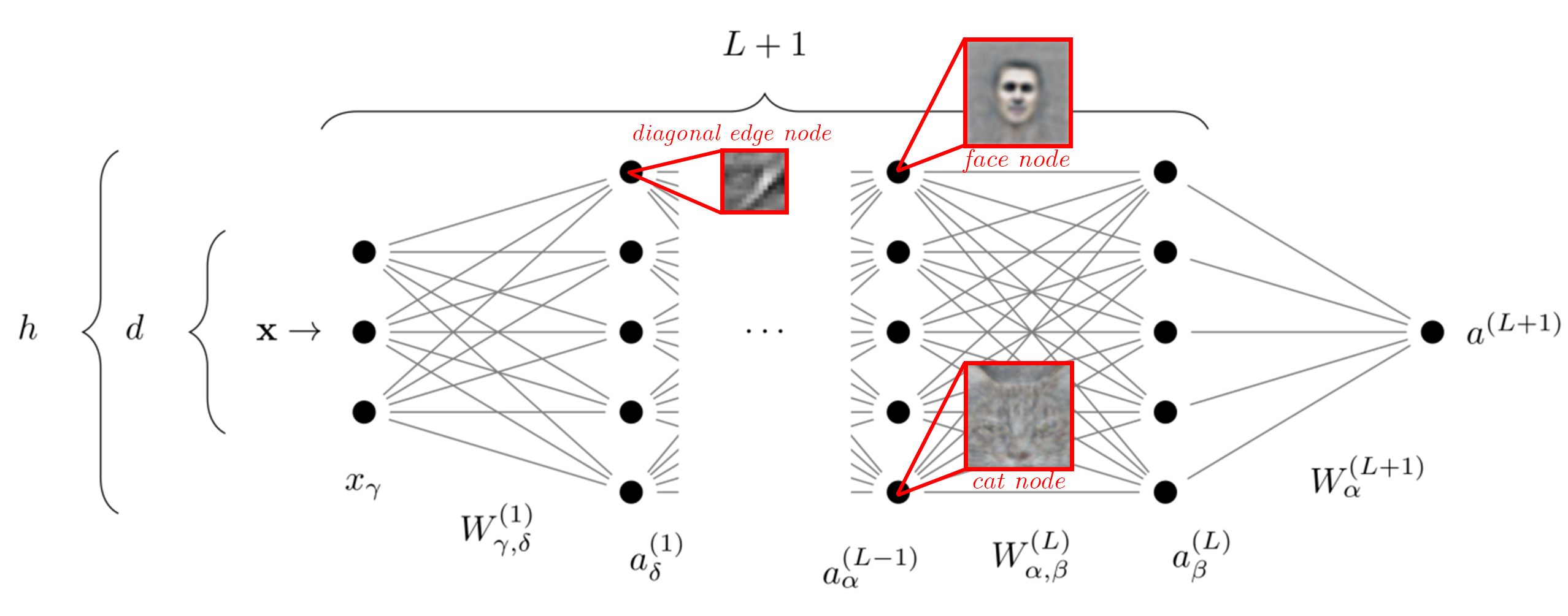
Figure 1: Architecture of a fully-connected network with $L$ hidden layers of neurons of constant size $h$. Points indicate neurons, connections between them are characterized by a weight. Biases are not represented here. The $W$’s are the weights, $\mathbf{x}$ is the input, and the $a$’s are the preactivations as defined in Equations (1-3). Taken from [8]. In red: Neural representation of the data at different depths (illustrative). Neurons in the first layers respond to local, simple features, such as edges. Deeper in the network, neurons respond to more and more high-level features such as cats or human faces. Adapted from [9].

For fully connected nets (FC) – which, from a theoretical point of view, are the most studied architectures – the output function can be written recursively as:

$$\tilde{f}_{\bf\theta}(\mathbf{x})\equiv a^{(L+1)},\vspace{0.5em}$$ (1)

$$a^{(i)}_{\beta}=\sum_{\alpha}\frac{1}{\sqrt{h}}W^{(i)}_{\alpha,\beta}\,\sigma\left(a^{(i-1)}_{\alpha}\right)+B^{(i)}_{\beta},$$ (2)

$$a^{(1)}_{\beta}=\sum_{\alpha}\frac{1}{\sqrt{d}}W^{(1)}_{\alpha,\beta}\,x_{\alpha}+B^{(1)}_{\beta},$$ (3)

where $a^{(i)}_{\alpha}$ is the preactivation of neuron $\alpha$, located at depth $i$ and $L$ the total number of layers. We consider networks with a fixed number of hidden layers $L$, each of size $h$. In the following, given that the total number of parameters follows $N\sim Lh^{2}$, we’ll use both $h$ and $N$ to refer to the network size. In our notation the set of parameters $\mathbf{\theta}$ includes both the weights $W^{(i)}_{\alpha,\beta}$ and the biases $B^{(i)}_{\alpha}$. $\sigma(z)$ is the non-linear activation function, e.g. the ReLU $\sigma(z)=\max(z,0)$. As is commonly done, we use the ”LeCun initialization” of the weights, for which they are scaled by a factor $1/\sqrt{h}$. It ensures that the limit of infinite width is not trivial, see e.g. discussions in [10]. We represent the network in Fig. 1.

Convolutional neural nets (CNNs), inspired from the primate brain, perform much better than FCs for a variety of tasks including image classification. Each hidden layer is composed of a number of channels, each representing the data as a feature map – itself an image. CNNs perform the same operations at distinct locations in the image, and enforce that these operations are local. CNNs are thus more constrained than FCs, and they can be obtained from the latter by imposing that some weights are identical (to enforce translational invariance) and others zero (to enforce locality).

Learning Dynamics

Weights are learnt by fitting the training set, which is done by minimising a loss or cost function ${\cal L}$. To simplify notations, we consider a binary classification problem, with a set of $P$ distinct training data denoted $\{(\mathbf{x}_{\mu},y_{\mu})\}_{\mu=1}^{P}$. The vector $\mathbf{x}_{\mu}$ is the input, which lives in a $d$-dimensional space, and $y_{\mu}=\pm 1$ is its label . ${\cal L}$ is a sum on all the training set of how each datum is well-fitted:

$$\mathcal{L}(\mathbf{\theta})=\frac{1}{P}\sum_{\mu=1}^{P}\ell(y_{\mu}f(\mathbf{x}_{\mu})),$$ (4)

where $f$ is a model and $\ell$ is a decreasing function of its argument. Popular choices include the linear ($\gamma=1$) or quadratic ($\gamma=2$) hinge loss $\ell(y_{\mu}f(\mathbf{x}_{\mu}))=\mathrm{max}\left(0,\Delta_{\mu}\right)^{\gamma}$ with $\Delta_{\mu}\equiv 1-y_{\mu}f(\mathbf{x}_{\mu})$, or the cross-entropy $\ell(y_{\mu}f(\mathbf{x}_{\mu}))=\log(1+\exp(-y_{\mu}f(\mathbf{x}_{\mu})))$. The hinge loss has the advantage that bringing the loss Eq.4 to zero is equivalent to satisfying a set of constraints $\Delta_{\mu}<0$, corresponding to fitting the data by a margin unity. This fact is the basis for the analogy with other satisfiability problems encountered in physics, as discussed below. This choice however does not influence significantly performance for SOTA architectures on usual benchmarks  [8].

Different procedures can then be used to minimise ${\cal L}$, starting from a random initialization of the weights (an important fact to keep in mind). In particular, gradient descent (GD) or stochastic gradient descent (SGD) are commonly used. For SGD, only a (changing) subset of the terms entering the sum of Eq.4 is considered at each minimisation time step. Various tricks can improve performance depending on the data considered, including early stopping (minimisation is stopped before the loss hits bottom) or weight decay (terms are then added to the loss to prevent weights to become too large).

Performance

Once learning is done, generalization performance can be estimated from a test set (data not used to train, but whose distribution is identical to the training set) by computing the probability to misclassify one new datum, the so-called test error $\epsilon$. How many data are needed to learn a task is characterized by the learning curve $\epsilon(P)\>$. Generally, it is observed that the test error is well described by a power law decay $P^{-\beta}$ in the range of training set size $P$ available with an exponent $\beta$ that depends jointly on the data and the algorithm chosen. In [11], $\beta$ is reported for SOTA architecture for several tasks: in neural-machine translation $\beta\approx 0.3$–$0.36$; in language modeling $\beta\approx 0.06$–$0.09$; in speech recognition $\beta\approx 0.3$ and in image classification (ImageNet) $\beta\approx 0.3$–$0.5$.

Deep nets learn a hierarchical representation of the data

Once learning took place, it is possible to analyse to which features in the data neurons respond mostly to [9, 12]. Strikingly, findings are very similar to what is found in the visual cortex of primates: neurons learn to respond to more and more abstract aspects of the data as the signal progresses through the network, as illustrated in Fig.1. This observation is believed to be an important aspect of why deep learning works, yet understanding how abstract features are learnt dynamically, and how much it contributes to performance, remains a challenge.

1.2 Why deep learning should not work

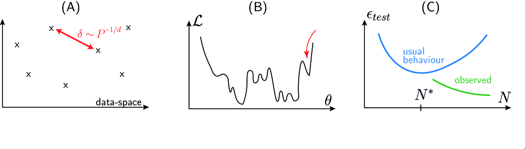
Figure 2: A: Curse of dimensionality. In high dimensions, every point lies far away from its neighbours, forbidding classification based on distances alone. B: Sketch of the loss landscape. Starting from a random initialization, the dynamics could get stuck in a bad minimum of the loss. C: Usual behaviour (blue line) of the test error as a function of the number of parameters, expected to be minimal when $N$ is of order of the smallest value $N^{*}$ where data can be fitted. Green: observations indicate that for deep learning, increasing the number of parameters generally improves behaviour, even in a regime where data are perfectly fitted.

Curse of dimensionality

General arguments suggest that $\beta$ should be extremely small — and learning thus essentially impossible — when the dimension $d$ of the data is large, which is generally the case in practice. For example in a regression task, if the only assumption on the target function is that it is Lipschitz continuous, then the test error cannot be guaranteed to decay faster than with an exponent $\beta\sim\nicefrac{{1}}{{d}}$ [13]. This curse of dimensionality [14] stems from the geometrical fact that the distance $\delta$ among nearest-neighbour data points decays extremely slowly in large $d$ as $\delta\sim P^{-\nicefrac{{1}}{{d}}}$, as depicted in the Fig.2.A. Thus, interpolation or classification methods based on distances are expected to be very imprecise for generic data.

Bad minima in the loss landscape

Another problem, which made deep learning less popular in the 90’s, concerns learning. The loss function has no guarantees to be convex, and the parameters space is high-dimensional. What prevents then the learning dynamics to get stuck in poorly performing minima with high loss, as sketched in Fig.2.B? In other words, under which conditions can one guarantee that training data are well fitted? Is the loss landscape similar to the energy landscape of glassy systems in physics, where the number of minima is exponential in the number of degrees of freedom [15, 16]?

Over-parametrization

Finally, neural nets are often trained in the over-parametrized regime, where the number of parameters $N$ is significantly larger than the number of data points $P$. In that regime, their capacity is very large: they can fit the training set even if labels are randomized [17]. Statistical learning theory then gives no guarantees that over-fitting does not occur, and that the model learnt has any predictive power. Indeed from statistics text books one expects a bell-shape learning curve relating the test error to the number of parameters of the model, as depicted in Fig.2.C. A very puzzling aspect of deep learning is that increasing $N$ passed the point where all data are perfectly fitted does not destroy predictive power, but instead improves it  [18, 19, 20, 21] as shown in Fig.2.

1.3 Current insights on these paradoxes

No bad minima in over-parametrized networks

Recently, it was realised that the landscape of deep learning is not glassy after all, if the number of parameters is sufficient. Theoretical works that focus on nets with a huge number of parameters (and one hidden layer), and empirical work with more realistic architectures  [22, 23, 24, 25], support that the loss function is characterized by a connected level set: any two points in parameter space with identical loss are connected by a path in which the loss is constant. Moreover, empirical studies of the curvature of the loss landscape (captured by the spectrum of the Hessian)  [26, 27, 28] and of SGD dynamics [29, 30] reveal that the landscape displays a large number of flat directions, even at its bottom. It is not the case for under-parametrized networks [30].

These observations raise key questions. Is there a phase transition in the landscape geometry as the number of parameters grows? If so, what is its universality class? How does it affect performance?

Implicit regularization and infinite width nets

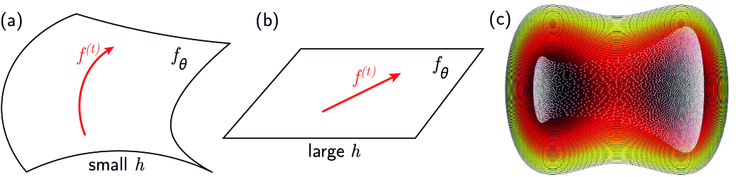
Figure 3: A: sketch of the dynamics in function space for a finite width net. As weights change the function evolves along the black manifold of expressible functions, which is curved. B: in the infinite width limit, this manifold becomes flat even though the function evolves by ${\cal O}(1)$: the relationship between function and weights became linear. C: interacting particles in a potential. When their number is large, describing their density instead of their individual motion becomes favorable (image graciously shared by Eric Vanden-Eijnden).

How can over-parametrized networks be predictive, if they can fit any data? It must imply that the GD or SGD dynamics lead to specific minima of the loss landscape where the function is more regular than for generic minima– a phenomenon coined implicit regularization [18, 19]. As sketched in Fig.2, performance is best as $N\rightarrow\infty$, triggering a huge interest in that limit. To which algorithms does GD correspond to in that case?

NTK: The propagation of the input signal through infinite-width FC nets at initialization is now well-understood. If the weights – defined in Eqs.3 – are initialized as i.i.d. random variables with zero mean and variance one (a set-up we consider throughout this work), the output function $\tilde{f}(x)$ is a Gaussian random process. Its covariance can be computed recursively [31, 32, 33, 34, 35, 36].

Very recently it was realised that the learning dynamics also simplifies in this limit  [10, 37, 38, 39, 40, 41]. The key insight of [10] is that the output becomes a linear function of the weights then, as sketched in Fig.3 A,B. Physically, very tiny changes of weights can interfere positively and change the output by ${\cal O}(1)$ which is sufficient to learn, but is not sufficient to change the gradient $\nabla_{\theta}\tilde{f}$.

More formally, the gradient flow dynamics at finite time can always be described by the neural tangent kernel (NTK) defined as:

$$\Theta(\theta,x,y)=\nabla_{\theta}\tilde{f}_{\theta}(x)\cdot\nabla_{\theta}\tilde{f}_{\theta}(y),$$ (5)

where $x,y$ are two inputs and $\nabla_{\theta}$ is the gradient with respect to the parameters $\theta$. Specifically, $\partial\tilde{f}(x)/\partial t$ can be expressed as a linear combination of the $\Theta(\theta,x,x_{i})$; i.e. $\tilde{f}$ evolves within a space of dimension $P$. In general, $\Theta$ depends on $\theta$ and thus on time and on the randomness of the initialization. Yet as $h\to\infty$, $\Theta(\theta,x,y)$ converges to a well-defined limit independent of initialization, and does not vary in time: deep learning in that limit is thus essentially a kernel method [10].

Feature learning (hydrodynamic) regime: The infinite width limit can be taken differently by adding a factor $1/\sqrt{h}$ in the definition of the output. Then the weights must change significantly for the output to become ${\cal O}(1)$ and fit the data. This recently discovered limit is called “mean field”, “rich” but also “feature learning regime” in the literature, because the neurons learn how to respond to different aspects of the input data, as in Fig.1 – whereas, in the NTK limit, the neuron’s response evolves infinitesimally. This regime has been studied in several works focusing mostly on one-hidden layer networks [42, 43, 44, 45, 46, 47, 48], with recent development for deeper nets, see e.g. [49]. In this setting the output function for a one hidden layer reads:

$$\tilde{f}_{\theta}(x)=\frac{1}{h}\sum_{i=1}^{h}W^{(2)}_{i}\sigma(\frac{1}{\sqrt{d}}W^{(1)}_{i}\cdot x+B_{i}),$$ (6)

The law of large number can then be invoked to replace Eq.6 by an integral:

$$\tilde{f}_{\theta}(x)\to\int\mathrm{d}W^{(2)}\mathrm{d}W^{(1)}\mathrm{d}B\,\rho(W^{(2)},W^{(1)},B)\;W^{(2)}\sigma(\frac{1}{\sqrt{d}}W^{(1)}\cdot x+B)$$ (7)

where $\rho$ is the density of parameters. It is then straightforward to show that gradient flow leads to a dynamics on $\rho$ of the usual type for conserved quantities: it is the divergence of a flux $\partial\rho/\partial t=-\nabla\cdot J$. Here the divergence is computed with respect to the set of weights associated with a single neuron, and the flux follows $J=\rho\Psi(W^{(2)},W^{(1)},B;\rho_{t})$ where $\Psi$ is some function that can be expressed in terms of the loss  [42]. This formulation is equivalent to the hydrodynamics description of interacting particles in some external potential. Fig.3.C illustrates that when the number of particles (or neurons) is large, $\rho$ is a more appropriate description than keeping track of all the particle positions (the weights in that case).

Lazy training: The fact that deep learning converges to well-defined algorithms as $h$ diverges, explains why performance converges to a well-defined value in that limit (which will depend on the limit considered), as sketched in Fig.2. Yet, this distinction between a regime where the NTK does not change, and one where it evolves and features are learnt can be made at finite $h$. Chizat and Bach proposed a model of the form [50]:

$$f_{\theta}(x)\equiv\alpha\left[\tilde{f}_{\theta}(x)-\tilde{f}_{\theta(t=0)}(x)\right],$$ (8)

$\alpha={\cal O}(1)$ corresponds to the NTK initialization and $\alpha={\cal O}(h^{-\nicefrac{{1}}{{2}}})$ to the mean-field limit. In the over-parametrised regime (our work below defines it sharply) where data are fitted, infinitesimal changes of weights are sufficient to learn when $\alpha\rightarrow\infty$ at finite $h$, and the NTK does not evolve in time (but has fluctuations at initialization). This regime is sometimes referred to as lazy training, in our context we will interchangeably denote it the NTK regime.

Overall, these findings are recent breakthrough in our understanding of neural nets. Yet they ask many questions that are central to this review. If two limits exist, which one best characterises neural networks that are used in practice? Which limit leads to a better performance? How does it depend on the architecture and data structure? Which effect causes the improvement of performance as $h$ increases?

Curse and invariance toward diffeomorphisms

Mallat and Bruna [51, 52] proposed that invariance toward smooth deformations of the image, i.e. diffeomorphisms, may allow deep nets to beat the curse of dimensionality. Specifically, consider the case where the input vector $x$ is an image. It can be thought as a function $x(s)$ describing intensity in position $s$, where $s\in[0,1]^{2}$ . A diffeomorphism is a bijective deformation that changes the location $s$ of the pixels to $s^{\prime}=\tau(s)$. In our review below, it will be useful to introduce the pixel displacement field $\xi(s)=\tau(s)-s$, analogous to the displacement field central to elasticity. We denote by $T_{\tau}[x]$ the image deformed by $\tau$, i.e. $T_{\tau}[x](s)=x(\tau^{-1}(s))$. One expects that smooth diffeomorphisms do not affect the label of an image: $Prob(y(x)\neq y(T_{\tau}[x]))\ll 1$ if $\|\nabla_{s}\xi\|\ll 1$.

Mallat and Bruna could handcraft CNNs, the ”scattering transform”, that are insensitive to smooth diffeomorphisms and perform well:

$$|f(x)-f(T_{\tau}[x])|\leq C_{0}\|\nabla_{s}\xi\|.$$ (9)

They hypothesised that during training, CNNs learn to satisfy Eq.9. In this view, by becoming insensitive to many aspects of the data irrelevant for the task, CNNs effectively reduce the data dimension and make the problem tractable.

A limitation of this framework is that it says little about how invariants are learnt dynamically. Yet, it is the center of the problem. FC nets are more expressive than CNNs, and nothing a priori prevents them from learning these invariants – yet, they presumably don’t, since their performance do not compare with CNNs. Along this route, an interesting question is how to develop observables to characterise empirically the dynamical emergence of invariants. Attempts have been made using mutual information approaches [53] which display problems in such a deterministic setting [54]; or measures based on the effective dimension of the neural representation of the data [55, 56] which are informative but can sometimes lead to counter-intuitive results . In Section 5 we discuss other observables based on kernel PCA of the NTK.

Figure 4: Phase diagram for the performance of deep learning in the width $h$ v.s. rescaled initialization magnitude $\tilde{\alpha}=\sqrt{h}\alpha$ plane, where $\alpha$ is defined in Eq.8. The architecture corresponds to a fully-connected neural network with two hidden layers trained with gradient descent [57]. Binary classification was performed for Left MNIST binary (odd/even) and Right CIFAR10 binary (classes have been regrouped in two sets). The training sets have been reduced to 5000 samples. These data sets were first projected on 10 and 30 PCAs, respectively. This dimensionality reduction of the problem is useful to study the jamming transitionbut not necessary to investigate the over-parametrized regime [57]. This choice does not affect qualitatively the geometry of the diagram however. The colormap shows the generalization of the ensemble average over 15 samples. The full black line indicates the cross-over from feature to lazy training. It is defined as the location for which the change of the NTK after training $\Delta\Theta=\Theta(t=\infty)-\Theta(0)$ is equal in norm to its magnitude at initialization, i.e. $\|\Delta\Theta\|/\|\Theta(0)\|=1$. Choosing other values for this ratio (see dashed lines) does not affect qualitatively the geometry of the cross-over line. The vertical color lines indicate the jamming transition where the training loss hits zero (in the black region the training loss does not reach zero). Its precise position depends on the time the simulation is allowed to run [8], as indicated in legend (using a GPU V100 and the gradient flow algorithm of [57] (gradient descent with adaptive learning rate)). It is expected and corresponds to the usual critical slowing down occurring near phase transitions. Horizontal dashed lines correspond to the measures done in Fig.5. The code used to generate these data is available at https://doi.org/10.5281/zenodo.4322828.

1.4 Organization of the manuscript

To think about the results above and the questions they raise in a unified manner, it is useful to consider Fig.7. It shows novel empirical data for the performance of neural nets in the plane $(h,\tilde{\alpha})$ where $h$ is the width and $\tilde{\alpha}$ the rescaled initialization amplitude $\tilde{\alpha}=\sqrt{h}\alpha$. Specifically, the ensemble test error of fully-connected nets learning MNIST (a data set of images of digits [58]) and CIFAR10 (images of planes, dogs, etc…) respectively with gradient descent is shown. This ensemble test error is computed by preparing, for each point in the phase diagram, $M=15$ nets with different initialization. The test error of the mean predictor $\langle f\rangle$ over the 15 trained nets is then shown. The black region corresponds to the under-parametrized regime where the loss of individual nets does not converge to zero after learning. As discussed below, its boundary corresponds to a line of critical points corresponding to a ”jamming transition” where the system stops displaying a rough landscape. In the colored over-parametrized regime, the black line indicates a cross-over separating the lazy training regime (where the total change of the NTK of individual nets during learning is small in relative terms) from a feature learning regime (where the NTK evolves significantly).

Fig.5 shows the curves for the test error and the ensemble test error for three values of $\tilde{\alpha}$, as $h$ varies. At the jamming transition, the test error displays a peak as observed in [59]. A similar peak occurs in regression problems [21], where it has a simpler origin and occurs when the number of parameters matches the number of data. This shape for the test error has since then been coined double-descent [60]. Interestingly, as shown in Fig.5 this phenomenon occurs independently of the value of $\tilde{\alpha}$ (and thus of the over-parametrized regime one enters into passed jamming) and vanishes when the ensemble average is taken, as observed in [61] and recently confirmed in [62].

Our goal is to review, in non-technical terms, concepts and arguments justifying such a phase diagram and discuss the learning of invariants in this context. In section 2, we will argue that the boundary of the black region in Fig.7 is a line of critical point, analogous to the jamming transition occurring in repulsive particles with finite-range interactions. For wider nets, the landscape is not glassy and displays many flat directions. We will provide a simple geometric argument justifying why this transition in deep nets fall into the universality classes of ellipsoid (rather than spherical) particles, which fixes the properties of the landscape (such as the spectrum of the Hessian) near the transition. We will mention an argument à la Landau justifying the cusp in the test error at that point. In Section 3, we will provide a quantitative explanation as to why the test error keeps improving as the width increases passed this transition. Increasing width turns out to eliminate the noise due to the random initialization of the weights, eventually leading to the well-defined algorithms introduced above. Ensemble averaging at finite width efficiently eliminates this source of noise as well as the double descent, as shown in Fig.5. In Section 4, we will explain why the cross-over between the lazy and feature learning regimes corresponds asymptotically to a flat line in Fig.7. We will review observations that lazy training outperforms feature learning for standard data sets of images for fully connected architectures, but not for CNNs architectures, corresponding to a larger learning curve exponent $\beta$. In Section 5, we review arguably the simplest model in which a neural net learns invariants in the data structure, by considering that labels do not depend on some directions in input space. As observed in real data, two distinct training exponents $\beta$ in the lazy and feature learning can then be computed. We conclude by discussing open questions.

Figure 5: Comparison of the generalization error and the ensemble generalization error for the same data, architecture and learning dynamics used in Fig.7. Values of $\tilde{\alpha}$ used are indicated in legends, and corresponds to the colored horizontal dashed lines in Fig.7. The ensemble average is done over 20 samples. The vertical lines indicate the location, or interval of locations, where the jamming transition occurs. Note that ensemble averaging improves a lot performance at intermediate width, and eliminates the double descent both in the lazy or feature learning regime.

2 Loss landscape and Jamming transition

Minimizing a loss is very similar to minimizing an energy. Describing the energy landscape of physical systems is a much studied problem, especially in the context of glasses. Progress was made on this topic in the last fifteen years by considering finite range interactions, for which bringing the energy to zero is equivalent to satisfying a set of constraints. In that case, the landscape is controlled by a critical point [63, 64, 65], the so-called jamming transition. It occurs as the particle density $\phi$ increases. For $\phi>\phi_{c}$, a gradient descent from a random initial positions of the particles gets stuck in one – out of many – meta-stable states, corresponding to a glassy solid as depicted in Fig.6B,D. For lower densities, the gradient descent reaches zero energy, as sketched in Fig.6.E : particles can freely move without restoring forces, and the landscape has many flat directions. It corresponds to the situations depicted in Fig.6A,C.

Figure 6: Sketch of the jamming transition for repulsive spheres and ellipses. (a,b,c,d) Both systems transition from a fluid to a solid as the density passes some threshold, noted $\phi_{S}$ for spheres and $\phi_{E}$ for ellipses. (e) For denser packings, the potential energy ${\cal U}$ becomes finite. (f) The ratio $N_{\Delta}/N$ between the number of particles in contact $N_{\Delta}$ (corresponding to unsatisfied constraints) and the number of degrees of freedom $N$ jumps discontinuously to a finite value, which is unity for spheres but smaller for ellipses. (g,h) This difference has dramatic consequence on the energy landscape, in particular on the spectrum of the Hessian. In both cases, the spectrum becomes non-zero at jamming, but it displays a delta function with finite weight for ellipses (indicating strictly flat directions), followed by a gap with no eigenvalues, followed by a continuous spectrum (h, full line). For spheres, there is no delta function nor gap (g, full line). As one enters the jammed phase, in both cases a characteristic scale $\lambda\sim\sqrt{{\cal U}}$ appears in the spectrum (g and h, dotted lines). From [8].

Figure 7: A Phase diagram indicating where the hinge loss hits zero (in blue) or not (in white) at the end of training, as the number of parameters $N$ and training points $P$ vary, for the MNIST data set discussed above (binary classification, 10 PCAs) trained with a FC nets with 3 hidden layers. B Number of unsatisfied patterns $N_{\Delta}/N$ as a function of the loss at the end of training, following the arrow indicated in panel A. Here $N$ is fixed, and $P=1,\dots 70k$. C The spectrum of the dominant term in the Hessian near jamming $H_{0}$ (averaged over the run at jamming, in the rectangle of B) presents a delta function in zero and a gaped continuous spectrum at high frequencies, a generic feature of hypostatic jamming. D Fluctuations of the output function along the arrow shown in A, averaged over 20 initial conditions. It decays asymptotically as a power-law $N^{-1/4}$ for the MNIST data set. At jamming, these fluctuations explode, consistent with a quadratic singularity. From [8, 61].

There are two universality classes for jamming, leading to distinct properties for the curvature of the landscape (i.e. the spectrum of the Hessian) [66, 67, 68, 69, 70, 71], for the structure of the packing obtained [72, 73, 74, 75] and for the dynamical response to a perturbation [76, 77]. Spheres and ellipses fall in distinct classes as illustrated in Fig.6. More generally, the jamming transition occurs generically in satisfiability problems with continuous degrees of freedom (it can be defined with discrete degrees of freedom [78], but then differs qualitatively; in particular, the present discussion does not apply to the discrete case). It occurs in the perceptron [79, 80, 81] but also for deep nets [8, 59].

We will recall below a geometric argument introduced in [8] determining the universality class of the jamming transition. For deep nets, jamming belongs to the universality class of ellipses [8, 59]. The spectrum of the loss near the jamming transition displays zero modes, a gap and a continuous part, as measured in Fig7.C. Another implication of this analogy is the number $N_{\Delta}$ of data whose margin is smaller than unity after learning, which contribute to the loss. These data are conceptually similar to the support vectors central to SVM algorithms. For particles, $N_{\Delta}$ corresponds the number of pairs of particles still overlapping after energy minimization. As illustrated in Fig7.B, $N_{\Delta}/N$ jumps from zero to a value strictly smaller than one at jamming where the loss becomes positive, precisely as ellipses do.

Geometric argument fixing the universality class:

Here we seek to give a simple intuition of the result of [8] (a more rigorous argument can be found there). We consider continuous satisfiability problems where one seeks to minimize an energy or loss function of the type:

$${\cal U}=\sum_{\mu\in m}\frac{1}{2}\Delta_{\mu}^{2}.$$ (10)

where the sum is made on all constraints that are not satisfied, corresponding to $\Delta_{\mu}>0$. The quantities $\Delta_{\mu}$ can depend in general on the $N$ degrees of freedom of the system. For systems of particles, ${\cal U}$ is an energy and $\Delta_{\mu}$ is the overlap between a pair $\mu=(i,j)$ of particles $i$ and $j$. For spheres it reads $\Delta_{ij}=2R-r_{ij}$ where $R$ is the particle radius and $r_{ij}=|\!|{\bf r}_{i}-{\bf r}_{j}|\!|$ the distance between particles $i$ and $j$. In that case, $N$ is the number of particles times the spatial dimension. For the perceptron or deep nets, ${\cal U}$ corresponds to a quadratic hinge loss generally denoted ${\cal L}$ defined in Eq.4 (it is straightforward to extend these arguments to other hinge losses with $\gamma>1$ [8, 63], the case $\gamma=1$ of the linear hinge shares many similarities with those but also display interesting differences [82]). As defined in the introduction, in that case $\Delta_{\mu}=1-f({\bf x}_{\mu})y_{\mu}$.

As the jamming transition is a singular point, it is useful – but not strictly necessary – to think of approaching from the glassy (large density $\phi$ or under-parametrized) phase. It corresponds to ${\cal U}\rightarrow 0$ as sketched in Fig. 6 E,F, implying that $\Delta_{\mu}\rightarrow 0$ $\forall\mu\in m$. As argued in [83], for each $\mu\in m$ the constraint $\Delta_{\mu}=0$ defines a manifold of dimension $N-1$. Satisfying $N_{\Delta}$ such equations thus generically leads to a manifold of solutions of dimension $N-N_{\Delta}$. Imposing that solutions exist thus implies that, at jamming, one has:

$$N_{\Delta}\leq N\,.$$ (11)

Note that this argument implicitly assumes that the $N_{\Delta}$ constraints are independent, see [8] for more discussions.

An opposite bound can be obtained by considerations of stability, by imposing that in a stable minimum the Hessian must be positive definite [66]. The Hessian is an $N\times N$ matrix which can be written as:

$${\cal H}_{U}=\sum_{\mu\in m}\nabla\Delta_{\mu}\otimes\nabla\Delta_{\mu}+\sum_{\mu\in m}\Delta_{\mu}{\cal H}_{\Delta_{\mu}}\equiv{\cal H}_{0}+{\cal H}_{p}\,,$$ (12)

where ${\cal H}_{\Delta_{\mu}}$ is the Hessian of $\Delta_{\mu}$, and ${\cal H}_{0}$ and ${\cal H}_{p}$ correspond to the first and second sum, respectively. ${\cal H}_{0}$ is positive semi-definite, since it is the sum of $N_{\Delta}$ positive semi-definite matrices of rank unity; thus ${\rm rk}({\cal H}_{0})\leq N_{\Delta}$, implying that the null-space of ${\cal H}_{0}$ is at least of dimension $N-N_{\Delta}$. ${\cal H}_{p}$ becomes very small approaching jamming, since the $\Delta_{\mu}$’s vanish. Let us denote by $N^{-}$ the number of negative eigenvalues of ${\cal H}_{p}$. Requiring that ${\cal H}_{U}$ has no negative eigenvalues thus implies:

$$N_{\Delta}\geq N^{-}\,.$$ (13)

For spheres [64] (as well as for the perceptron if a negative margin is used while constraining the norm of the weight vector), ${\cal H}_{p}$ is negative definite and $N^{-}=N$. This results stems from the fact that ${\cal H}_{\Delta_{\mu}}$ is negative semi-definite. Indeed ${\cal H}_{\Delta_{\mu}}$ characterizes the second order change of overlap between particles, and is negative because the distance between spheres moving transversely to their relative direction always increase following Pythagoras theorem. In that case we thus have $N_{\Delta}\geq N$. Together with Eq. (11) that leads to $N_{\Delta}=N$: as spheres jam the number of degrees of freedom and the number of constraints (stemming from contacts) are equal, as empirically observed [63]. This property is often called isostaticity.

However, in other problems such as ellipses and deep nets, ${\cal H}_{\Delta_{\mu}}$ and thus ${\cal H}_{p}$ have positive eigenvalues. Indeed the overlap between two ellipses can increase if one of them rotates. Likewise, for a fully-connected Relu net and random data at initialization, ${\cal H}_{p}$ has a symmetric spectrum and $N^{-}\approx N/2$. Generically one expects then jamming to occur with $N_{\Delta}<N$ as sketched for ellipses in Fig.6 and shown empirically for neural nets learning MNIST in Fig.7. Jamming is then referred to as ”hypostatic”. The associated consequences on the spectrum of the hessian shown on the same figures are derived in specific cases in [84, 69, 68]: it always presents a delta function in zero and a gap at jamming.

Effect of the number of training data $P$

The location of the jamming transition $N^{*}(P)$ depends on $P$. This dependence is linear for random data but sub-linear for structured data [8], as exemplified in Fig.7.A. Denoting $N^{-}=C_{0}N$, and using Eq.13 together with $N_{\Delta}\leq P$, we obtain $N^{*}(P)\leq P/C_{0}$, guaranteeing convergence to a zero loss for a number of parameters linear in $P$ if $C_{0}>0$. We conjecture that $C_{0}$ to remain bounded by a strictly positive value for large $N$ for generic data and architectures used in practice . $C_{0}$ can be measured a posteriori, leading to the bound corresponds to the dotted line in Fig.7.A. $C_{0}$ a priori depends on the choice of architecture, dynamics and data set. Controlling its value a priori is yet out of reach , and would lead to a rather tight guarantee of convergence toward a global minimum of the loss.

Effect of the scale of initialization $\tilde{\alpha}$

It is apparent in Fig.7 that the location of the jamming transition depends on the scale of initialization $\tilde{\alpha}$. From this figure, we observe the following general trend: the jamming transition occurs with less parameters when the test error of the ensemble-averaged predictor is small. It follows the intuition that an easier rule to learn should correspond to less parameters to fit the data.

Effect of the Jamming transition on performance

As the jamming transition is approached, the norm $\|f_{N}\|$ of the predictor diverges [8], which is responsible in the cusp in the double descent displayed by the test error in Fig.5. This divergence was first pointed out for regression [21]. Yet for classification, the divergence defers quantitatively and is compatible with an inverse power-law, as illustrated in Fig.7.D. It can be understood using an argument à la Landau, inspired by results on the perceptron [79, 81]. The intuitive idea is that, by increasing the norm of the predictor, one reduces effectively the unit margin required by the hinge loss to fit the data. For $N<N^{*}$, data cannot be fitted even with a vanishing margin.

Specifically, consider that the norm of the predictor $\|f_{N}\|$ is fixed during training and denote by $N^{*}(\epsilon)$ the jamming transition as a function of the margin $\epsilon$. Assume (as occurs for the perceptron) that $N^{*}(\epsilon)$ is a smooth function of $\epsilon$, such that $N^{*}(\epsilon)\approx N^{*}(0)+N^{\prime*}(0)\epsilon$. For $N$ just above $N^{*}(0)$, margins of magnitude unity cannot be fitted for a fixed norm of the predictor, but they can if that norm is allowed to increase by a factor $N^{\prime*}(0)/(N-N^{*}(0))$. Indeed it effectively reduces the margin by that amount to some effective value $\tilde{\epsilon}\equiv\epsilon(N-N^{*}(0))/N^{\prime*}(0)$. By construction, $\tilde{\epsilon}$ satisfies $N^{*}(\tilde{\epsilon})=N$. This argument justifies the observed inverse power-law.

Note that any perturbation to gradient flow (such as early stopping, using stochastic gradient descent or weight decay) will destroy this divergence . Such regularizations are thus most efficient near jamming [59].

3 Double descent and the benefits of overparametrization

To avoid bad minima in the loss landscape, it is thus sufficient to crank up $N$ passed $N^{*}$. But then, one would naively expect to lower performance and overfit, as illustrated in the right panel of Fig.2. It is not the case for classification and deep nets, as illustrated in Fig.5: performance is very poor and displays a cusp right at the jamming transition point $N^{*}$, and then continuously improves as $N\rightarrow\infty$!

A scaling theory can be built to explain quantitatively why performance keeps improving with $N$ passed that point, and how fast the test error reaches its asymptotic behavior [61]. Essentially, at infinite width learning corresponds to well-defined algorithms as discussed in introduction, but these algorithms become noisier when the width is finite. Indeed as $N\sim h^{2}$ increases, the fluctuations on the learnt output function induced by the random initialization of the weights decrease [86]. It follows $\|f_{N}-\langle f_{N}\rangle\|\sim N^{-1/4}$ as shown in Fig.7.D, where $\langle f_{N}\rangle$ is obtained by ensemble-averaging outputs trained with different random initializations. This result is true both for the lazy training [61] and the feature learning [57] regime, as justified below. The associated increase in test error is quadratic in the fluctuations (it is obvious for a mean square error loss, but is also true for classification under reasonable assumptions [61]), leading to $\langle\epsilon(f_{N})\rangle-\epsilon(\langle f_{N}\rangle)\sim N^{-1/2}$ as observed [61]. This effect is responsible for the double descent, as can be directly checked by considering the training curve $\epsilon(\langle f_{N}\rangle)$ of the ensemble average function $\langle f_{N}\rangle$ in Fig.5 which does not display a second descent. More generally as apparent in Fig.7, at fixed $\tilde{\alpha}=\sqrt{h}\alpha$, the ensemble average test error weakly varies with $h$ once in the over-parametrized regime.

In the lazy training regime, the fluctuations $\langle\|f_{N}-\langle f_{N}\rangle\|\rangle\sim N^{-1/4}$ simply mirror the fluctuations of the NTK induced by initialization, argued to follow $\|\Theta_{N}-\langle\Theta_{N}\rangle\|\sim N^{-1/4}\sim h^{-1/2}$ in [61], as analytically confirmed since then [87, 88]. For simple losses and gradient descent, the predictor $f_{N}$ must acquire the same fluctuations [61], as observed.

Similar fluctuations induced by initial conditions $\langle\|f_{N}-\langle f_{N}\rangle\|\rangle\sim N^{-1/4}$ with identical consequences occur in the feature learning regimes in neural nets [57]. Such fluctuations are certainly expected at initialization for a one-hidden layer, since the density of neurons parameters $\rho$ introduced in Eq.7 must have finite sampling fluctuations of order $\delta\rho\sim 1/\sqrt{h}\sim N^{-1/4}$ as expected from the central limit theorem. Because in the asymptotic regime $N\rightarrow\infty$ the value of $\rho$ at initialization affects the learnt function, the magnitude of fluctuations $\delta\rho$ (and thus of the learnt function $f_{N}$) induced by the random initialization will still scale as $N^{-1/4}$ after learning, as rigorously proven for a one-hidden layer in [89].

Overall, this scaling theory supports that for generic data sets and deep architectures, the second descent results from the noise induced by finite $N$ effects and initialization on the limiting algorithms reached as $N\rightarrow\infty$. One interesting practical implication, apparent in Fig.7 and Fig.5, is that optimal performance is found by ensemble averaging nets of limited width passed their jamming transition.

Since these arguments were proposed, the double descent curve has been analytically computed in the simple case of linear data in the limit of infinite dimension and random features machines [46, 90], where it was also shown [91, 92] to result from the fluctuations of the kernel that vanish with increasing number of neurons, confirming the present explanation.

Figure 8: Left, Center: Ensemble-average test error vs. the scaling parameter $\tilde{\alpha}=\sqrt{h}\alpha$. It illustrates that the NTK regime (large $\sqrt{h}\alpha$) tends to outperform the feature learning regime (small $\sqrt{h}\alpha$) for FC architecture (Left) but not in CNNs (Center). In the latter case, the training curve exponent $\beta$ is larger in the feature learning (blue curve, $\beta\approx 1/2$) regime than in the NTK one (orange curve, $\beta\approx 1/3$). From [57].

4 Disentangling the NTK and feature learning regimes

As discussed in the previous section, wider nets are more predictive. A comparable gain of performance can however be obtained already at intermediate width, by ensemble averaging outputs over multiple initialization of the weights. As apparent in Fig.7, the rescaled magnitude of initialization $\tilde{\alpha}=\alpha\sqrt{h}$ which allows to cross-over between the lazy training and feature learning regimes does affect performance. Which regime best characterises deep nets used in practice? Which one performs better? Some predictions of the NTK regime appear to hold in realistic architectures  [39], and training nets in NTK limit can achieve good performance on real datasets [40, 93, 94]. Yet, in several cases the feature learning regime beats the NTK [95, 50], in line with the common idea that building an abstract representation of the data such as sketched in Fig.1 is useful. Several theoretical works show that NTK under-performs for specific, simple models of data [96, 97, 14, 98, 99].

In [57], this question was investigated systematically for deep nets in the $(\alpha,h)$ plane, where $\alpha$ is the scale of initialization introduced in [50] as defined in Eq.8. This study developed numerical methods of adaptive learning rates to follow gradient flow while changing $\alpha$ by ten decades. The main results are as follows:

(i) The cross-over between the two regimes occur when $\alpha\sqrt{h}=O(1)$ as apparent in Fig.7, extending the result of [50] limited to one hidden layer nets. For $\alpha\sqrt{h}\ll 1$, $\|\Delta\Theta\|/\|\Theta\|\gg 1$ while the opposite holds true when $\alpha\sqrt{h}\gg 1$. Here $\Delta\Theta=\Theta(t)-\Theta(t=0)$ characterises the evolution of the tangent kernel and $t$ is the learning time. It is convenient to divide the loss by $\alpha^{2}$ and consider $\tilde{\cal L}\equiv{\cal L}/\alpha^{2}$, which can be shown to ensure that the dynamics occurs on a time scale independent of $\alpha$ in the large $\alpha$ limit [50, 57]. This result holds true for the usual choices of loss (cross-entropy, hinge, etc…) at any finite time. It also holds true for $t\rightarrow\infty$ if the hinge loss is used, since in that case convergence to a zero loss occurs in finite time independently of $h$ and $\alpha$.

Here we provide a schematic argument justifying this result, see [57] for a more detailed analysis. The variation of the output $f$ with respect to the pre-activation $a$ (which are of order one at initialization) of a given neuron is of order $\partial f/\partial a\sim\alpha/\sqrt{h}$. This result is obvious for the last hidden layer (using that the last weights are of order $1/\sqrt{h}$), but can be justified recursively at all layers, as discussed in [57] and derived implicitly in the NTK study [10]. For gradient flow, the variation $\Delta a$ of pre-activation due to the evolution of the bias (considering the previous weights leads to a similar scaling) must be of order $\Delta a\sim t(\partial\tilde{\cal L}/\partial f)(\partial f/\partial a)\sim t/\alpha\sqrt{h}$ using that $\partial\tilde{\cal L}/\partial f\sim 1/\alpha^{2}$. Thus $\Delta a$ is of order $1/\alpha\sqrt{h}$ at the end of training (since a zero hinge loss is reached on a time scale $t=O(1)$). The NTK regime must thus break down when $\Delta a\sim 1$ when the relation between weights and output must become non-linear, corresponding to a cross-over for $\alpha^{*}\sim 1/\sqrt{h}$ for large $h$.

A similar line of thought can be used at intermediate width. When reducing $h$ so as to approach the jamming transition from the over-parametrized phase, the norm of the output – and therefore weights and pre-activations – explode as reviewed in Section 2. One is never then in the lazy training regime, and the relationship between the variation of weights and the output must become non-linear. Thus, in the vicinity of the jamming transition, the networks always lie in the feature learning regime. Consequently, the cross-over lines separating lazy and feature learning must bend up and never cross the jamming line in Fig.7. We do observe curves qualitatively bending up as expected (yet it is hard to make precise measurements very close to jamming).

(ii) For fully-connected nets and gradient descent, the NTK tends to outperform the feature learning regime, as exemplified in the Left panel of Fig.8. This result was found for a variety of data sets (MNIST, Fashion-MNIST, CIFAR10, etc…), except for MNIST 10 PCA. It is apparent in Fig.7, where the best performance for MNIST 10 PCA appears to occur the cross-over region $\tilde{\alpha}\sim 1$.

(iii) For CNN architectures, feature learning outperforms the NTK regime as shown in the central panel of Fig.8. It corresponds to a larger training curve exponent $\beta$, as appears in the right panel of Fig.8. (ii,iii) were recently confirmed by the Google team [62].

These observations raise various questions. What are the advantages and drawbacks of feature learning, and why are the latter more apparent in FC rather than CNN architectures? For modern CNN architectures, is the improvement of the learning curve exponent $\beta$ in the feature learning regime key to understand how the curse of dimensionality is beaten? Is it associated with learning invariants in the data? In our opinion, the answers to these questions are yet unknown. To start tackling these questions, in the next section we study a simple model of invariant data for which the improvement of the learning curve exponent $\beta$ in the feature learning regime can be computed.

5 Learning simple invariants by compressing irrelevant input dimensions

How can the curse of dimensionality be beaten?

A favorable aspect of various data sets such as images is that the data distribution $P(\bf x)$ is very anisotropic, consistent with the notion that the data lie in a manifold of lower dimension. In that case, the distance between neighboring data reduces faster with growing $P$, improving kernel methods [100]. The positive effect of a moderate anisotropy can also be shown for kernel classification [101] and regression [99, 102]. Yet, even in simple data sets like MNIST of CIFAR10, the intrinsic dimensions remain significant ($d_{int}\approx 14$ and $d_{int}\approx 30$ respectively [100]). This effect helps but cannot resolve the curse of dimensionality for complex data set: indeed using Laplace or Gaussian kernels (which are very similar to the NTK of fully connected nets) lead to $\beta\approx 0.4$ for MNIST (which is decent) but $\beta\approx 0.1$ for CIFAR10, which implies very slow learning as the number of data increases.

As discussed in the introduction, another popular idea is that data sets as images are learnable because they display many invariant transformations that leave the labels unchanged. By becoming insensitive to those, the network essentially reduces the dimension of the data. This view is consistent with the notion that deep learning leads to an abstract neural representation of the data sketched in Fig.1. This effect may be responsible for our observation in the right panel of Fig.8 that the training curve exponent $\beta$ is more favorable in the feature learning regime. However, understanding how invariants are built dynamically and how it affects performance and $\beta$ remains a challenge.

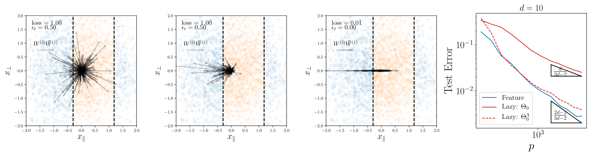
Figure 9: Left: Distribution of the weights vectors ${\vec{W}}^{(1)}$ pondered by the neuron second weight $W^{(2)}$ shown at different time points during the learning process (as characterised by the value of the loss in legend) for the stripe model. It reveals an alignment of the first layer of weight vectors in the informative direction. Training data points are also shown, and coloured depending on their labels. Right: Training curve $\epsilon(P)$ of a one hidden layer in the feature learning regime (blue), the NTK regime (red) and the NTK regime after compressing the data in the perpendicular direction by the factor $\Lambda$ (dashed red). Note the similarity between this curve and the blue one, supporting that the main effect of learning feature for these data is the geometric compression of uninformative directions in input space. From [103].

Specific models of data can be built [43, 104, 90, 99] in which lazy training does not learn at all, whereas neural nets trained in the feature learning regime succeed. These models however do not capture the two finite and distinct learning curve exponents $\beta$ observed in the two regimes.

The stripe model

In [96, 103, 101], a simple model of invariant is considered. The labels do not depend on $d_{\perp}=d-d_{\parallel}$ directions of input space, so that $y(x)=y(x_{\parallel})$ where $x=(x_{\perp},x_{\parallel})$. $x_{\bot}$ could correspond for example to uninformative pixels near the boundaries of pictures. For gradient descent, with the logistic loss, a one-hidden layer can be shown to correspond to a max-margin classifier in a certain non-Hilbertian space of functions [96]. Dimension-independent guarantees on performance can then be obtained if the data can be separated after projection in a low dimensional space. The analysis is rigorous and general, but requires to go to extremely long times not used in practice and does not predict values for $\beta$.

In [103, 101], the hinge loss is considered. In that case, the dynamics stops after a reasonable time. If the density of data points does not vanish at the interface between labels, and if the latter is sufficiently smooth (e.g. planar or cylindrical), it is found that the test error decays as a power law in both regimes. For the lazy training regime, scaling arguments inspired by electrostatics lead to $\beta_{Lazy}=d/(3d-2)$. Feature learning performs better, as one find $\beta_{Feature}=(d+\nicefrac{{d_{\perp}}}{{2}})/(3d-2)$. The key effect leading to an improvement of the feature learning regime is illustrated in Fig.9 for $d_{\parallel}=1$, called the stripe model: due to the absence of gradient in the orthogonal direction, the weights only grow along the $d_{\parallel}$ dimensions. Thus, for a infinitesimal initialization of the weights ($\alpha\rightarrow 0$), the neurons align along the informative coordinate in the data. Accordingly, in relative terms, they become less sensitive to $x_{\perp}$, which merely acts as a source of noise. This denoising is limited by the finite size of the training set. Specifically, it is found that $\Lambda\equiv W_{\parallel}/W_{\perp}\sim\sqrt{P}$ where $W_{\parallel}$ and $W_{\perp}$ are the characteristic scales of the first layer of weights in the informative and uninformative directions respectively. This effect is equivalent to a geometrical compression of magnitude $\Lambda$ of the input in the uninformative direction. Indeed performing this compression by considering the transformed data $(x_{\parallel},x_{\perp}/\Lambda)$, and learning these in the NTK regime gives very similar performance as learning the original data in the feature regime, see the right panel of Fig.9.

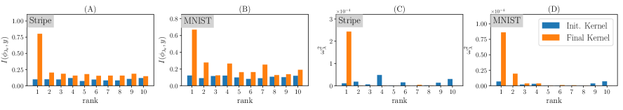
Figure 10: Relationship between the kernel PCA of the NTK (obtained both at initialization and after learning) and the labels. The mutual information (characterizing the amount of correlation) between the top eigenvectors of the Gram matrix and the labels (A, B) and their projection $\omega_{\lambda}$ (C, D) get large after learning for both the stripe model (learnt with a FC with one hidden-layer) and MNIST (learnt with a CNN). From [103].

Kernel PCA of the NTK reveals a geometric compression of invariants

The stripe models illustrates that neural nets in the feature learning regime can learn to become insensitive to transformations in the data that do not affect the labels. This insensitivity is limited by the sampling noise associated with a finite data set. Is this phenomenon also occurring for more modern architectures and more subtle invariants characterizing images? Measurements of the intrinsic dimension of the neural representation of data [55, 56] or mutual information estimates [53] suggest that it may be so, but as mentioned in introduction these observables have some limitations.

In the feature learning regime, the NTK evolves in time. This evolution leads to a better kernel for the task considered. Indeed, using a kernel method based on the NTK obtained at the end of training leads to essentially identical performance than the neural net itself [103]. This observation is consistent with previous ones showing that the NTK ”improves” in time [105, 106], in the following sense. For kernels we can always write $\Theta(x,y)=\psi(x)\cdot\psi(y)$, where $\psi(x)$ is a vector of features. In the case of the NTK, $\psi(x)$ can be chosen as the gradient of the output $f$ with respect to the weights – see Eq.5. Kernels tend to perform better [107] if the vector of labels $\{y(x_{i})\}_{i=1...P}$ has large coefficients along the first PCAs of the features vectors $\{\psi(x_{i})\}_{i=1...P}$ (an operation called kernel PCA [108]). Such an alignment between the first PCAs of the features vectors of the NTK and the vector of labels is observed during learning [105, 106].

Although there is no general theory as to why such an alignment occurs, the stripe model provides a plausible explanation for this effect. In that case, this improvement must occur because one evolves from an isotropic kernel to an anisotropic one with diminished sensitivity to uninformative directions $x_{\perp}$. As a result, the top kernel PCA becomes more informative on the label (Fig.10.A) on which they project more (Fig.10.C). The same result is observed for a CNN trained on MNIST as shown in Fig.10.B,D. Overall, this view support that the improvement of the NTK reveals the geometric compression of uninformative directions in the data.

6 Conclusion

Don’t be afraid of bad minima! Just crank-up the number of parameters until you pass a jamming transition. Beyond that point, bad minima are not encountered, and you can bring the loss to zero. Depending on the network width and on how you scale the value of your function at initialization, deep learning can then behave as a kernel method, or can alternatively learn features. Simple scaling arguments delimit the corresponding phase diagram, and appear to hold for benchmark data sets. Remarkably, these arguments depend very little on the specific data considered. Their practical implication is that ensemble averaging nets with different initialization past the jamming transition can be an effective procedure, as found by different groups [61, 57, 62].

Taking into account where you are in this phase diagram is arguably key to understand outstanding questions on deep learning. It is true for example for the role of stochasticity in the dynamics, which appears to improve performance. It is natural that using stochastic gradient descent instead of gradient flow will help near jamming, because the noise will regularize the divergence of the predictor norm – an effect that can already be obtained with early stopping [59]. Likewise, for repulsive particles temperature regularizes singularity near the jamming transition [109]. Yet, it would be useful to study its effect on performance for the distinct regions of the phase diagram. It would be particularly interesting to know if one of the main effects of stochasticity in the over-parametrized limit is to push upward the cross-over between the lazy and feature learning regime in Fig.7, thus improving performance in CNNs where feature learning outperforms lazy training.

Ultimately, the central question left to understand is performance, and how the curse of dimensionality is beaten in deep nets. Even at an empirical level, the idea that invariance toward diffeomorphisms is the central phenomenon behind this success is not established. At the theoretical level, this view as not been combined with the recent improvement of our understanding of learning, which as mostly focused on fully connected nets. In comparison, the effort to model how CNNs learn features is more modest, despite that only those architectures tend to work well in practice. Such studies would arguably require to design simple canonical models of data presenting complex invariants, which are currently scarce.

Acknowledgments

We acknowledge G. Biroli, S. d’Ascoli, F. Cagnetta, A. Favero, F. Gabriel, C. Hongler, A. Jacot, J. Paccolat, L. Pillaud-Vivien, S. Spigler, L. Sagun, U. Tomasini, K. Tyloo and all members of the PCSL group for discussions. This work was partially supported by the grant from the Simons Foundation (#454953 Matthieu Wyart). M.W. thanks the Swiss National Science Foundation for support under Grant No. 200021-165509.

References

- [1] David Marr and Tomaso Poggio. A computational theory of human stereo vision. Proceedings of the Royal Society of London. Series B. Biological Sciences, 204(1156):301–328, 1979.
- [2] Yann LeCun, Yoshua Bengio, and Geoffrey Hinton. Deep learning. Nature, 521(7553):436, 2015.
- [3] Dario Amodei, Sundaram Ananthanarayanan, Rishita Anubhai, Jingliang Bai, Eric Battenberg, Carl Case, Jared Casper, Bryan Catanzaro, Qiang Cheng, Guoliang Chen, et al. Deep speech 2: End-to-end speech recognition in english and mandarin. In International conference on machine learning, pages 173–182, 2016.
- [4] Baoguang Shi, Xiang Bai, and Cong Yao. An end-to-end trainable neural network for image-based sequence recognition and its application to scene text recognition. IEEE transactions on pattern analysis and machine intelligence, 39(11):2298–2304, 2016.
- [5] Brody Huval, Tao Wang, Sameep Tandon, Jeff Kiske, Will Song, Joel Pazhayampallil, Mykhaylo Andriluka, Pranav Rajpurkar, Toki Migimatsu, Royce Cheng-Yue, et al. An empirical evaluation of deep learning on highway driving. arXiv preprint arXiv:1504.01716, 2015.
- [6] David Silver, Julian Schrittwieser, Karen Simonyan, Ioannis Antonoglou, Aja Huang, Arthur Guez, Thomas Hubert, Lucas Baker, Matthew Lai, Adrian Bolton, et al. Mastering the game of go without human knowledge. nature, 550(7676):354–359, 2017.
- [7] Volodymyr Mnih, Koray Kavukcuoglu, David Silver, Alex Graves, Ioannis Antonoglou, Daan Wierstra, and Martin Riedmiller. Playing atari with deep reinforcement learning. arXiv preprint arXiv:1312.5602, 2013.
- [8] Mario Geiger, Stefano Spigler, Stéphane d’Ascoli, Levent Sagun, Marco Baity-Jesi, Giulio Biroli, and Matthieu Wyart. Jamming transition as a paradigm to understand the loss landscape of deep neural networks. Physical Review E, 100(1):012115, July 2019. Publisher: American Physical Society.
- [9] Quoc V Le. Building high-level features using large scale unsupervised learning. In 2013 IEEE international conference on acoustics, speech and signal processing, pages 8595–8598. IEEE, 2013.
- [10] Arthur Jacot, Franck Gabriel, and Clément Hongler. Neural tangent kernel: Convergence and generalization in neural networks. In Proceedings of the 32Nd International Conference on Neural Information Processing Systems, NIPS’18, pages 8580–8589, USA, 2018. Curran Associates Inc.
- [11] Joel Hestness, Sharan Narang, Newsha Ardalani, Gregory Diamos, Heewoo Jun, Hassan Kianinejad, Md Patwary, Mostofa Ali, Yang Yang, and Yanqi Zhou. Deep learning scaling is predictable, empirically. arXiv preprint arXiv:1712.00409, 2017.
- [12] Bolei Zhou, Aditya Khosla, Agata Lapedriza, Aude Oliva, and Antonio Torralba. Object detectors emerge in deep scene cnns. arXiv preprint arXiv:1412.6856, 2014.
- [13] Ulrike von Luxburg and Olivier Bousquet. Distance-based classification with lipschitz functions. Journal of Machine Learning Research, 5(Jun):669–695, 2004.
- [14] Francis Bach. Breaking the curse of dimensionality with convex neural networks. The Journal of Machine Learning Research, 18(1):629–681, 2017.
- [15] Ludovic Berthier and Giulio Biroli. Theoretical perspective on the glass transition and amorphous materials. Reviews of Modern Physics, 83(2):587, 2011.
- [16] Anna Choromanska, Mikael Henaff, Michael Mathieu, Gérard Ben Arous, and Yann LeCun. The loss surfaces of multilayer networks. In Artificial Intelligence and Statistics, pages 192–204, 2015.
- [17] Chiyuan Zhang, Samy Bengio, Moritz Hardt, Benjamin Recht, and Oriol Vinyals. Understanding deep learning requires rethinking generalization. 5th International Conference on Learning Representations, ICLR 2017, Toulon, France, April 24-26, 2017, Conference Track Proceedings, 2017.
- [18] Behnam Neyshabur, Ryota Tomioka, Ruslan Salakhutdinov, and Nathan Srebro. Geometry of optimization and implicit regularization in deep learning. arXiv preprint arXiv:1705.03071, 2017.
- [19] Behnam Neyshabur, Zhiyuan Li, Srinadh Bhojanapalli, Yann LeCun, and Nathan Srebro. Towards understanding the role of over-parametrization in generalization of neural networks. arXiv preprint arXiv:1805.12076, 2018.
- [20] Yamini Bansal, Madhu Advani, David D Cox, and Andrew M Saxe. Minnorm training: an algorithm for training overcomplete deep neural networks. arXiv preprint arXiv:1806.00730, 2018.
- [21] Madhu S. Advani, Andrew M. Saxe, and Haim Sompolinsky. High-dimensional dynamics of generalization error in neural networks. Neural Networks, September 2020.
- [22] C Daniel Freeman and Joan Bruna. Topology and geometry of deep rectified network optimization landscapes. International Conference on Learning Representations, 2017.
- [23] Elad Hoffer, Itay Hubara, and Daniel Soudry. Train longer, generalize better: closing the generalization gap in large batch training of neural networks. In Advances in Neural Information Processing Systems, pages 1729–1739, 2017.
- [24] Daniel Soudry and Yair Carmon. No bad local minima: Data independent training error guarantees for multilayer neural networks. arXiv preprint arXiv:1605.08361, 2016.
- [25] Yaim Cooper. The loss landscape of overparameterized neural networks. arXiv preprint arXiv:1804.10200, 2018.
- [26] Levent Sagun, Léon Bottou, and Yann LeCun. Singularity of the hessian in deep learning. International Conference on Learning Representations, 2017.
- [27] Levent Sagun, Utku Evci, V. Uğur Güney, Yann Dauphin, and Léon Bottou. Empirical analysis of the hessian of over-parametrized neural networks. ICLR 2018 Workshop Contribution, arXiv:1706.04454, 2017.
- [28] Andrew J Ballard, Ritankar Das, Stefano Martiniani, Dhagash Mehta, Levent Sagun, Jacob D Stevenson, and David J Wales. Energy landscapes for machine learning. Physical Chemistry Chemical Physics, 2017.
- [29] Zachary C Lipton. Stuck in a what? adventures in weight space. International Conference on Learning Representations, 2016.
- [30] Marco Baity-Jesi, Levent Sagun, Mario Geiger, Stefano Spigler, Gerard Ben Arous, Chiara Cammarota, Yann LeCun, Matthieu Wyart, and Giulio Biroli. Comparing dynamics: Deep neural networks versus glassy systems. In Jennifer Dy and Andreas Krause, editors, Proceedings of the 35th International Conference on Machine Learning, volume 80 of Proceedings of Machine Learning Research, pages 314–323, Stockholmsmässan, Stockholm Sweden, 10–15 Jul 2018. PMLR.
- [31] Radford M. Neal. Bayesian Learning for Neural Networks. Springer-Verlag New York, Inc., Secaucus, NJ, USA, 1996.
- [32] Christopher KI Williams. Computing with infinite networks. In Advances in neural information processing systems, pages 295–301, 1997.
- [33] Jae Hoon Lee, Yasaman Bahri, Roman Novak, Samuel S. Schoenholz, Jeffrey Pennington, and Jascha Sohl-Dickstein. Deep neural networks as gaussian processes. ICLR, 2018.
- [34] Alexander G. de G. Matthews, Jiri Hron, Mark Rowland, Richard E. Turner, and Zoubin Ghahramani. Gaussian process behaviour in wide deep neural networks. In International Conference on Learning Representations, 2018.
- [35] Roman Novak, Lechao Xiao, Yasaman Bahri, Jaehoon Lee, Greg Yang, Daniel A. Abolafia, Jeffrey Pennington, and Jascha Sohl-dickstein. Bayesian deep convolutional networks with many channels are gaussian processes. In International Conference on Learning Representations, 2019.
- [36] Greg Yang. Scaling limits of wide neural networks with weight sharing: Gaussian process behavior, gradient independence, and neural tangent kernel derivation. arXiv preprint arXiv:1902.04760, 2019.
- [37] Simon S. Du, Xiyu Zhai, Barnabas Poczos, and Aarti Singh. Gradient descent provably optimizes over-parameterized neural networks. In International Conference on Learning Representations, 2019.
- [38] Zeyuan Allen-Zhu, Yuanzhi Li, and Zhao Song. A Convergence Theory for Deep Learning via Over-Parameterization. In International Conference on Machine Learning, pages 242–252. PMLR, May 2019. ISSN: 2640-3498.
- [39] Jaehoon Lee, Lechao Xiao, Samuel Schoenholz, Yasaman Bahri, Roman Novak, Jascha Sohl-Dickstein, and Jeffrey Pennington. Wide Neural Networks of Any Depth Evolve as Linear Models Under Gradient Descent. In H. Wallach, H. Larochelle, A. Beygelzimer, F. d\textquotesingle Alché-Buc, E. Fox, and R. Garnett, editors, Advances in Neural Information Processing Systems 32, pages 8572–8583. Curran Associates, Inc., 2019.
- [40] Sanjeev Arora, Simon S Du, Wei Hu, Zhiyuan Li, Russ R Salakhutdinov, and Ruosong Wang. On Exact Computation with an Infinitely Wide Neural Net. In H. Wallach, H. Larochelle, A. Beygelzimer, F. d\textquotesingle Alché-Buc, E. Fox, and R. Garnett, editors, Advances in Neural Information Processing Systems 32, pages 8141–8150. Curran Associates, Inc., 2019.
- [41] Daniel Park, Jascha Sohl-Dickstein, Quoc Le, and Samuel Smith. The Effect of Network Width on Stochastic Gradient Descent and Generalization: an Empirical Study. In International Conference on Machine Learning, pages 5042–5051. PMLR, May 2019. ISSN: 2640-3498.
- [42] Song Mei, Andrea Montanari, and Phan-Minh Nguyen. A mean field view of the landscape of two-layer neural networks. Proceedings of the National Academy of Sciences, 115(33):E7665–E7671, August 2018. Publisher: National Academy of Sciences Section: PNAS Plus.
- [43] Grant M Rotskoff and Eric Vanden-Eijnden. Neural networks as interacting particle systems: Asymptotic convexity of the loss landscape and universal scaling of the approximation error. arXiv preprint arXiv:1805.00915, 2018.
- [44] Lénaïc Chizat and Francis Bach. On the Global Convergence of Gradient Descent for Over-parameterized Models using Optimal Transport. In Advances in Neural Information Processing Systems 31, pages 3040–3050. Curran Associates, Inc., 2018.
- [45] Justin Sirignano and Konstantinos Spiliopoulos. Mean Field Analysis of Neural Networks: A Law of Large Numbers. SIAM Journal on Applied Mathematics, 80(2):725–752, January 2020. Publisher: Society for Industrial and Applied Mathematics.
- [46] Song Mei, Theodor Misiakiewicz, and Andrea Montanari. Mean-field theory of two-layers neural networks: dimension-free bounds and kernel limit. In Conference on Learning Theory, pages 2388–2464. PMLR, June 2019. ISSN: 2640-3498.
- [47] Phan-Minh Nguyen. Mean field limit of the learning dynamics of multilayer neural networks. arXiv preprint arXiv:1902.02880, 2019.
- [48] Justin Sirignano and Konstantinos Spiliopoulos. Mean field analysis of neural networks: A central limit theorem. Stochastic Processes and their Applications, 130(3):1820–1852, 2020.
- [49] Phan-Minh Nguyen and Huy Tuan Pham. A rigorous framework for the mean field limit of multilayer neural networks. arXiv preprint arXiv:2001.11443, 2020.
- [50] Lenaic Chizat, Edouard Oyallon, and Francis Bach. On lazy training in differentiable programming. In Advances in Neural Information Processing Systems, pages 2937–2947, 2019.
- [51] Joan Bruna and Stéphane Mallat. Invariant scattering convolution networks. IEEE transactions on pattern analysis and machine intelligence, 35(8):1872–1886, 2013.
- [52] Stéphane Mallat. Understanding deep convolutional networks. Philosophical Transactions of the Royal Society A: Mathematical, Physical and Engineering Sciences, 374(2065):20150203, 2016.
- [53] Ravid Shwartz-Ziv and Naftali Tishby. Opening the black box of deep neural networks via information. arXiv preprint arXiv:1703.00810, 2017.
- [54] Andrew M Saxe, Yamini Bansal, Joel Dapello, Madhu Advani, Artemy Kolchinsky, Brendan D Tracey, and David D Cox. On the information bottleneck theory of deep learning. Journal of Statistical Mechanics: Theory and Experiment, 2019(12):124020, 2019.
- [55] Alessio Ansuini, Alessandro Laio, Jakob H Macke, and Davide Zoccolan. Intrinsic dimension of data representations in deep neural networks. In Advances in Neural Information Processing Systems, pages 6111–6122, 2019.
- [56] Stefano Recanatesi, Matthew Farrell, Madhu Advani, Timothy Moore, Guillaume Lajoie, and Eric Shea-Brown. Dimensionality compression and expansion in deep neural networks. arXiv preprint arXiv:1906.00443, 2019.
- [57] Mario Geiger, Stefano Spigler, Arthur Jacot, and Matthieu Wyart. Disentangling feature and lazy training in deep neural networks. Journal of Statistical Mechanics: Theory and Experiment, 2020(11):113301, November 2020. Publisher: IOP Publishing.
- [58] Yann LeCun and Corinna Cortes. MNIST handwritten digit database. 2010.
- [59] S. Spigler, M. Geiger, S. d’Ascoli, L. Sagun, G. Biroli, and M. Wyart. A jamming transition from under- to over-parametrization affects generalization in deep learning. Journal of Physics A: Mathematical and Theoretical, 52(47):474001, October 2019. Publisher: IOP Publishing.
- [60] Mikhail Belkin, Daniel Hsu, Siyuan Ma, and Soumik Mandal. Reconciling modern machine-learning practice and the classical bias–variance trade-off. Proceedings of the National Academy of Sciences, 116(32):15849–15854, 2019.
- [61] Mario Geiger, Arthur Jacot, Stefano Spigler, Franck Gabriel, Levent Sagun, Stéphane d’Ascoli, Giulio Biroli, Clément Hongler, and Matthieu Wyart. Scaling description of generalization with number of parameters in deep learning. Journal of Statistical Mechanics: Theory and Experiment, 2020(2):023401, February 2020. Publisher: IOP Publishing.
- [62] Jaehoon Lee, Samuel S Schoenholz, Jeffrey Pennington, Ben Adlam, Lechao Xiao, Roman Novak, and Jascha Sohl-Dickstein. Finite versus infinite neural networks: an empirical study. arXiv preprint arXiv:2007.15801, 2020.
- [63] Corey S. O’Hern, Leonardo E. Silbert, Andrea J. Liu, and Sidney R. Nagel. Jamming at zero temperature and zero applied stress: The epitome of disorder. Phys. Rev. E, 68(1):011306–011324, Jul 2003.
- [64] M. Wyart. On the rigidity of amorphous solids. Annales de Phys, 30(3):1–113, 2005.
- [65] Andrea J Liu, Sidney R Nagel, W Saarloos, and Matthieu Wyart. The jamming scenario - an introduction and outlook. OUP Oxford, 06 2010.
- [66] Matthieu Wyart, Leonardo E Silbert, Sidney R Nagel, and Thomas A Witten. Effects of compression on the vibrational modes of marginally jammed solids. Physical Review E, 72(5):051306, 2005.
- [67] Eric DeGiuli, Adrien Laversanne-Finot, Gustavo Alberto Düring, Edan Lerner, and Matthieu Wyart. Effects of coordination and pressure on sound attenuation, boson peak and elasticity in amorphous solids. Soft Matter, 10(30):5628–5644, 2014.
- [68] Silvio Franz, Giorgio Parisi, Pierfrancesco Urbani, and Francesco Zamponi. Universal spectrum of normal modes in low-temperature glasses. Proceedings of the National Academy of Sciences, 112(47):14539–14544, 2015.
- [69] Carolina Brito, Harukuni Ikeda, Pierfrancesco Urbani, Matthieu Wyart, and Francesco Zamponi. Universality of jamming of nonspherical particles. Proceedings of the National Academy of Sciences, 115(46):11736–11741, November 2018. Publisher: National Academy of Sciences Section: Physical Sciences.
- [70] Mitch Mailman, Carl F. Schreck, Corey S. O’Hern, and Bulbul Chakraborty. Jamming in systems composed of frictionless ellipse-shaped particles. Phys. Rev. Lett., 102(25):255501, Jun 2009.
- [71] Z. Zeravcic, N. Xu, A. J. Liu, S. R. Nagel, and W. van Saarloos. Excitations of ellipsoid packings near jamming. Europhys. Lett., 87(2):26001, 2009.
- [72] Matthieu Wyart. Marginal stability constrains force and pair distributions at random close packing. Physical review letters, 109(12):125502, 2012.
- [73] Edan Lerner, Gustavo During, and Matthieu Wyart. Low-energy non-linear excitations in sphere packings. Soft Matter, 9:8252–8263, 2013.
- [74] Patrick Charbonneau, Jorge Kurchan, Giorgio Parisi, Pierfrancesco Urbani, and Francesco Zamponi. Fractal free energy landscapes in structural glasses. Nature Communications, 5(3725), 2014.
- [75] Patrick Charbonneau, Jorge Kurchan, Giorgio Parisi, Pierfrancesco Urbani, and Francesco Zamponi. Exact theory of dense amorphous hard spheres in high dimension. iii. the full replica symmetry breaking solution. Journal of Statistical Mechanics: Theory and Experiment, 2014(10):10009, 2014.
- [76] Edan Lerner, Gustavo Düring, and Matthieu Wyart. A unified framework for non-brownian suspension flows and soft amorphous solids. Proceedings of the National Academy of Sciences, 109(13):4798–4803, 2012.
- [77] E DeGiuli, G Düring, E Lerner, and M Wyart. Unified theory of inertial granular flows and non-brownian suspensions. Physical Review E, 91(6):062206, 2015.
- [78] Florent Krzakala and Jorge Kurchan. Landscape analysis of constraint satisfaction problems. Physical Review E, 76(2):021122, 2007.
- [79] Silvio Franz and Giorgio Parisi. The simplest model of jamming. Journal of Physics A: Mathematical and Theoretical, 49(14):145001, 2016.
- [80] Silvio Franz, Giorgio Parisi, Maxime Sevelev, Pierfrancesco Urbani, and Francesco Zamponi. Universality of the sat-unsat (jamming) threshold in non-convex continuous constraint satisfaction problems. SciPost Physics, 2(3):019, 2017.
- [81] Silvio Franz, Sungmin Hwang, and Pierfrancesco Urbani. Jamming in Multilayer Supervised Learning Models. Physical Review Letters, 123(16):160602, October 2019. Publisher: American Physical Society.
- [82] Silvio Franz, Antonio Sclocchi, and Pierfrancesco Urbani. Critical jammed phase of the linear perceptron. Physical Review Letters, 123(11):115702, 2019.
- [83] Alexei V. Tkachenko and Thomas A. Witten. Stress propagation through frictionless granular material. Phys. Rev. E, 60(1):687–696, Jul 1999.
- [84] Matthieu Wyart. Scaling of phononic transport with connectivity in amorphous solids. EPL (Europhysics Letters), 89(6):64001, 2010.
- [85] Arthur Jacot, Franck Gabriel, and Clément Hongler. The asymptotic spectrum of the hessian of dnn throughout training. arXiv preprint arXiv:1910.02875, 2019.
- [86] Brady Neal, Sarthak Mittal, Aristide Baratin, Vinayak Tantia, Matthew Scicluna, Simon Lacoste-Julien, and Ioannis Mitliagkas. A modern take on the bias-variance tradeoff in neural networks. arXiv preprint arXiv:1810.08591, 2018.
- [87] Boris Hanin and Mihai Nica. Finite depth and width corrections to the neural tangent kernel. arXiv preprint arXiv:1909.05989, 2019.
- [88] Ethan Dyer and Guy Gur-Ari. Asymptotics of wide networks from feynman diagrams. arXiv preprint arXiv:1909.11304, 2019.
- [89] Zhengdao Chen, Grant Rotskoff, Joan Bruna, and Eric Vanden-Eijnden. A Dynamical Central Limit Theorem for Shallow Neural Networks. Advances in Neural Information Processing Systems, 33, 2020.
- [90] Behrooz Ghorbani, Song Mei, Theodor Misiakiewicz, and Andrea Montanari. Linearized two-layers neural networks in high dimension. arXiv preprint arXiv:1904.12191, 2019.
- [91] Stéphane D’Ascoli, Maria Refinetti, Giulio Biroli, and Florent Krzakala. Double Trouble in Double Descent: Bias and Variance(s) in the Lazy Regime. In International Conference on Machine Learning, pages 2280–2290. PMLR, November 2020. ISSN: 2640-3498.
- [92] Arthur Jacot, Berfin Simsek, Francesco Spadaro, Clement Hongler, and Franck Gabriel. Implicit Regularization of Random Feature Models. In International Conference on Machine Learning, pages 4631–4640. PMLR, November 2020. ISSN: 2640-3498.
- [93] Sanjeev Arora, Simon S. Du, Zhiyuan Li, Ruslan Salakhutdinov, Ruosong Wang, and Dingli Yu. Harnessing the Power of Infinitely Wide Deep Nets on Small-data Tasks. September 2019.
- [94] Vaishaal Shankar, Alex Fang, Wenshuo Guo, Sara Fridovich-Keil, Jonathan Ragan-Kelley, Ludwig Schmidt, and Benjamin Recht. Neural Kernels Without Tangents. In International Conference on Machine Learning, pages 8614–8623. PMLR, November 2020. ISSN: 2640-3498.
- [95] Blake Woodworth, Suriya Gunasekar, Jason D. Lee, Edward Moroshko, Pedro Savarese, Itay Golan, Daniel Soudry, and Nathan Srebro. Kernel and Rich Regimes in Overparametrized Models. In Conference on Learning Theory, pages 3635–3673. PMLR, July 2020. ISSN: 2640-3498.
- [96] Lénaïc Chizat and Francis Bach. Implicit Bias of Gradient Descent for Wide Two-layer Neural Networks Trained with the Logistic Loss. In Conference on Learning Theory, pages 1305–1338. PMLR, July 2020. ISSN: 2640-3498.
- [97] Gilad Yehudai and Ohad Shamir. On the power and limitations of random features for understanding neural networks. In Advances in Neural Information Processing Systems, pages 6598–6608, 2019.
- [98] Behrooz Ghorbani, Song Mei, Theodor Misiakiewicz, and Andrea Montanari. Limitations of lazy training of two-layers neural network. In Advances in Neural Information Processing Systems, pages 9111–9121, 2019.
- [99] Behrooz Ghorbani, Song Mei, Theodor Misiakiewicz, and Andrea Montanari. When Do Neural Networks Outperform Kernel Methods? Advances in Neural Information Processing Systems, 33, 2020.
- [100] Stefano Spigler, Mario Geiger, and Matthieu Wyart. Asymptotic learning curves of kernel methods: empirical data versus teacher–student paradigm. Journal of Statistical Mechanics: Theory and Experiment, 2020(12):124001, December 2020. Publisher: IOP Publishing.
- [101] Jonas Paccolat, Matthieu Wyart, and Stefano Spigler. How isotropic kernels perform on simple invariants. Machine Learning: Science and Technology, 2020.
- [102] Sebastian Goldt, Marc Mézard, Florent Krzakala, and Lenka Zdeborová. Modeling the Influence of Data Structure on Learning in Neural Networks: The Hidden Manifold Model. Physical Review X, 10(4):041044, December 2020. Publisher: American Physical Society.
- [103] Jonas Paccolat, Leonardo Petrini, Mario Geiger, Kevin Tyloo, and Matthieu Wyart. Geometric compression of invariant manifolds in neural nets. arXiv preprint arXiv:2007.11471, 2020.
- [104] Greg Ongie, Rebecca Willett, Daniel Soudry, and Nathan Srebro. A Function Space View of Bounded Norm Infinite Width ReLU Nets: The Multivariate Case. April 2020.
- [105] Samet Oymak, Zalan Fabian, Mingchen Li, and Mahdi Soltanolkotabi. Generalization guarantees for neural networks via harnessing the low-rank structure of the jacobian. arXiv preprint arXiv:1906.05392, 2019.
- [106] Dmitry Kopitkov and Vadim Indelman. Neural Spectrum Alignment: Empirical Study. Artificial Neural Networks and Machine Learning – ICANN 2020, 2020.
- [107] Blake Bordelon, Abdulkadir Canatar, and Cengiz Pehlevan. Spectrum Dependent Learning Curves in Kernel Regression and Wide Neural Networks. In International Conference on Machine Learning, pages 1024–1034. PMLR, November 2020. ISSN: 2640-3498.
- [108] Bernhard Scholkopf, Alexander Smola, and Klaus-Robert Müller. Kernel principal component analysis. In Advances in Kernel Methods - Support Vector Learning, pages 327–352. MIT Press, 1999.
- [109] Eric Degiuli, E Lerner, and M Wyart. Theory of the jamming transition at finite temperature. The Journal of chemical physics, 142(16):164503, 2015.