Transition to turbulence in randomly packed porous media; scale estimation of vortical structures

Abstract

Pore-scale observation of vortical flow structures in porous media is a significant challenge in many natural and industrial systems. Vortical structure dynamics is believed to be the driving mechanism in the transition regime in porous media based on the pore Reynolds number, $Re_{p}$. To examine this assertion, a refractive-index matched randomly packed porous medium with homogeneously-sized glass spheres ($D_{B}=15\rm mm$) is designed to measure the scale of vortical flow structures in transition from unsteady laminar to turbulent using two-dimensional time-resolved particle image velocimetry. Planar Particle Image Velocimetry (PIV) data is used to quantify the scale of these structures with regard to size, strength, and number density using two different scalings (i) $Re_{p}$ macroscopic (global), and (ii) $Re_{\langle p\rangle}$ microscopic (local, pore-scale). Data is obtained for $Re_{p}$ from 100 to 948 in six different locations from the center of the bed towards the wall (one bead diameter away from wall). Direct measurement of vortex scale is quantified by employing swirl strength ($\lambda_{ci}$), vortex core ($\varGamma_{\tiny{2}}$), and enhanced swirl strength ($\lambda_{cr}/\lambda_{ci}$) vortex identification methods. These scales are compared with turbulent integral scales. Due to the confinement of the random medium, the inertia-dependent topology of the flow creates shear-dominant vortical structures in moderate unsteady laminar Reynolds numbers ($Re_{p}<300$), while the swirl-dominant flow structures appear in weak turbulent Reynolds numbers ($Re_{p}>500$). From the macroscopic point of view, (i) the size of vortical structures decreases asymptotically to reach 20$\%$ of the global hydraulic diameter, (ii) the strength of vortices increases monotonically by enhancing the inertial effects of $Re_{p}$, and (iii) the average number density of vortical structures grows from unsteady laminar to fully turbulent. From the pore-scale (local) point of view using $Re_{\langle p\rangle}$, (i) the size of vortical structures decreases monotonically with increasing local Reynolds number, (ii) the strength of vortices rises with $Re_{\langle p\rangle}$, and (iii) the number density of vortical structures for different $Re_{\langle p\rangle}$ is invariant relative to the pore size. These findings suggest pore versus macro-scale coupling exists for the scale of vortical flow structures in the transition regime, albeit the scale variation of pore-scale flow structures with local inertial effects is different from the asymptotic values captured in the macroscopic level with increasing $Re_{p}$.

I Introduction

Porous media flows have received increased attention in various natural and industrial applications over the past four decades. Depending upon the conditions, the flow may stay laminar or transition where unsteady chaotic behavior is seen at the pore spaces. Laminar flow in porous media has been extensively investigated in diverse industrial and natural processes. On the other hand, turbulent flows has lately been explored in a wide range of applications that also includes transition regime. This regime is observed in diverse disciplines including (1) near-surface environmental flow such as natural and urban canopies as well as fractured rocks and dams [1, 2, 3, 4, 5, 6, 7, 8, 9], (2) catalytic systems [10, 11, 12, 13, 14], (3) nuclear pebble bed reactors [15], (4) heat transfer enhancement in packed beds [16, 17, 18, 19, 20, 21, 22, 23], (5) dense fluidized beds [24, 25, 26], (6) flow in biological porous media [27, 28], (7) chromatography columns [29], (8) enhanced oil recovery [30, 31], and (9) thin porous media in paper making industry [32, 33]. These diverse applications demonstrate the need for further study of the transition whether the flow naturally becomes turbulent or is actively enhanced to increase performance.

The transition to turbulence in porous media may appear in a number of ways; (i) global (macroscopic) versus local (pore-scale) development of flow inertia [34, 35], (ii) flow heterogeneity leading to non-uniform distribution of flow in a porous bed [36], (iii) intrinsic flow instabilities [37, 38], and (iv) emergence of coherent topological patterns. These patterns [39, 40, 41, 38, 36, 42, 43, 44, 45] evolve spatially and temporally with inertial dominance in transition to turbulence and contribute to the change of scales. Furthermore, the complex structural geometry at the pore-level [46, 47, 48] results in generation of coherent topological regions such as recirculation zones, jet-like flows, channel-like flows, or impinging flows, as it has been seen by Patil and Liburdy [49], and Suekane et al. [34], and also regions resembling convergent-divergent nozzles, diffusers, wakes, or stagnant zones inside pores. Swirling structures can develop in these regions, which may evolve into turbulent eddies [50]. To understand proper scales during transition, it is essential to demarcate the viscous-inertial effects on the spatio-temporal evolution of scales. This process can be seen from a macroscopic (global) point of view (defined in Refs. 51, 52, 46) by neglecting the intrinsic flow characteristics. However, pore-scale (local) investigation of local transition is required to understand the overall transition process in randomly packed beds.

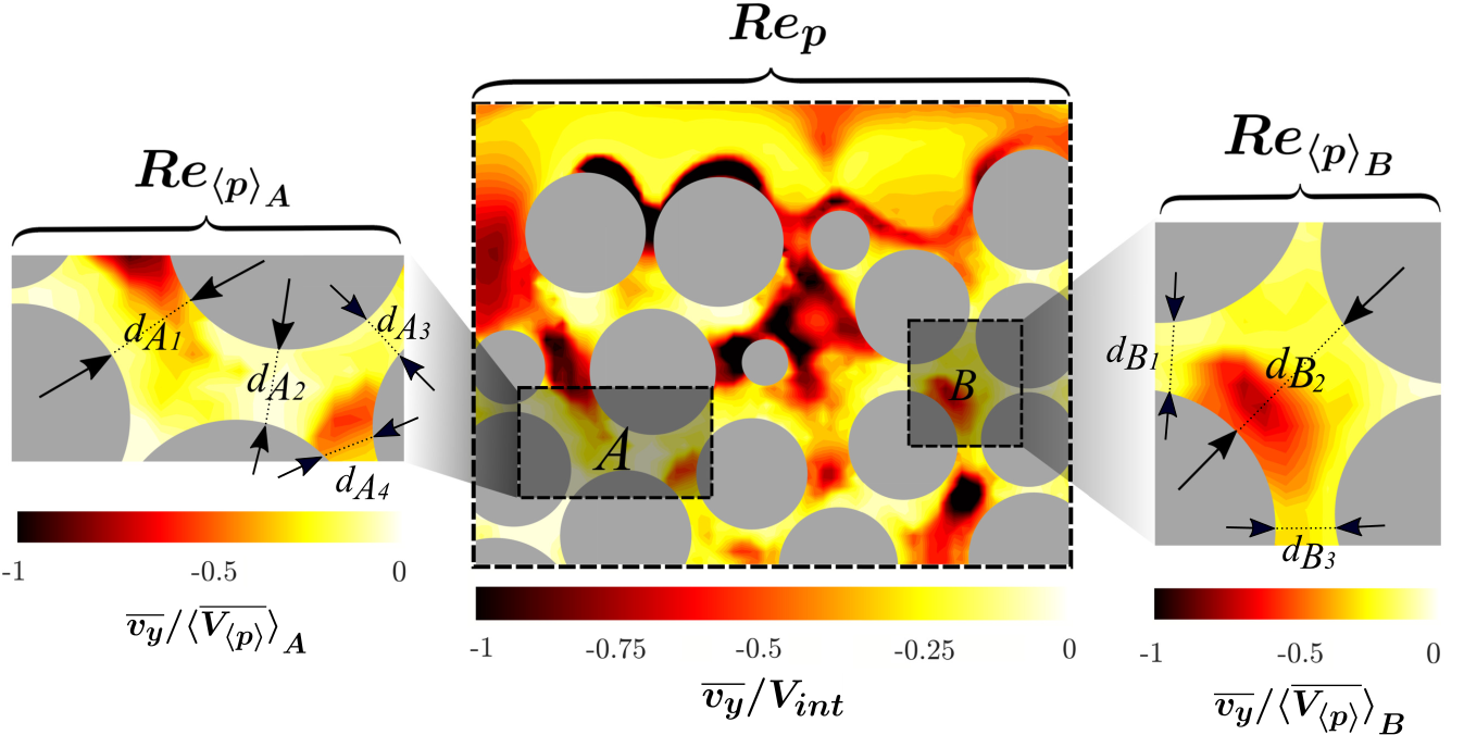
Figure 1: Schematic of the geometrical demonstration of individual pore-scale (local) regions for estimating the local Reynolds number $Re_{\langle p\rangle}$ versus global (macroscopic) for longitudinal (y-direction) velocity intensities normalized by interstitial velocity globally, and by pore-averaged velocity locally. Color bars represent the global and local velocity intensities.

Reynolds numbers have had different definitions among porous media community (Wood et al. 2020 [53]). These are listed as (i) particle diameter and superficial velocity [54, 55, 56, 57, 58, 14, 59, 60, 61, 62, 11, 63], (ii) pore hydraulic diameter and interstitial velocity [64, 49, 65, 66, 67, 68, 69, 70, 71, 33, 72, 73], (iii) approximate permeability and average intrinsic velocity [74, 75], (iv) pore-averaged velocity and particle size [41, 40, 38, 37, 76, 77, 78, 79, 42], and (v) pore-averaged length scale, and pore-averaged velocity. For the latter, the length scale has been based on the square root of pore area (Sederman et al. 1998 [36]), cross-stream length of velocity profile (Johns et al. 2000 [35]), or along a line perpendicular to the flow direction (Suekane et al. 2003 [34]). Use of a pore-averaged velocity with some measure of particle size has been applied extensively in regular packed beds [54, 76, 38, 40, 37] to perform comparisons with flow over sphere as a canonical case [80, 81, 82, 83, 84, 85, 86, 87, 88]. However, this method overestimates actual pore sizes in random packings.

In this study, two Reynolds numbers are used to investigate the scale characteristics for pore-scale versus macroscopic perspectives. The global Reynolds number ($Re_{p}$) uses method (ii) above and is defined as:

$$Re_{p}=\frac{V_{int}D_{H}}{\nu}$$ (1)

where, $V_{int}$ is the interstitial velocity defined as a function of superficial or seepage velocity (also known as Darcy velocity) as $V_{int}=V_{Darcy}/\Phi$, $D_{H}$ is the hydraulic diameter defined based on the bead diameter and porosity as $D_{H}=\Phi D_{B}/(1-\Phi)$, and $\nu$ is the kinematic viscosity of the fluid. The local pore-scale Reynolds number $Re_{\langle p\rangle}$ is defined here to compensate for the deficiencies of applying hydraulic diameter as the length scale of each arbitrary pore in estimating the actual pore-scale flow inertia and to better define local pore-scale velocities. Hence,

$$Re_{\langle p\rangle}=\frac{\langle\overline{V_{\langle p\rangle}}\rangle\langle d_{\langle p\rangle}\rangle}{\nu}$$ (2)

where, (—) indicates temporal averaging, $\langle\rangle$ represents spatial averaged over a single pore, such that $\langle\overline{V_{\langle p\rangle}}\rangle$ is the temporally and spatially averaged velocity for a single pore the entire fluid phase as shown in Figure 1, $\langle d_{\langle p\rangle}\rangle$ is the local pore length scale spatially averaged in the fluid phase in ten locations of pores perpendicular to the local velocity profile (as shown in Figure 1), and $\nu$ is kinematic viscosity of fluid.

Investigating the macroscopic scaled flow physics in porous media during transition regimes has led to transition predictions in the literature [89, 55, 90, 91, 58, 92, 74, 60, 29, 66]. These studies have investigated the transition to turbulence with considerable differences in their finding for the range of transition. These estimates of the onset of turbulence are based on the premise of interpreting a micro-scale phenomena with macroscopic parameters (pressure, hydraulic conductivity, macroscopic dispersion, permeability, and mass transfer) or models (Darcy-Forchheimer) [77].

Many studies have considered microscopic flow investigation using highly resolved experimental observations, or numerical simulations to identify flow structures for detecting the pore-scale flow physics during the transition, as is shown in Figure LABEL:fig:3. These studies predict the following regimes: (i) steady laminar ($29<Re_{p}<193$), (ii) unsteady laminar ($46<Re_{p}<156$), (iii) steady inertial ($1<Re_{p}<148$), (iv) unsteady inertial ($148<Re_{p}<300$), (v) viscous-inertial transition ($78<Re_{p}<480$), and (vi) turbulent ($159<Re_{p}<727$). The deviations between these predictions are very wide [93, 54, 90, 56, 91, 14, 94, 61, 60, 62]. The disparity of these predictions provides motivation to study the entire regime ($100<Re_{p}<948$) to identify the scale of vortical structures in this range for a different perspective of scale evolution in transition. Non-invasive imaging techniques to measure local velocity in porous media have been applied for several decades, with high resolution capabilities recently developed.
[ floatPos=!htbp!, capWidth=h, capPos=after, capAngle=90, objectAngle=90, capVPos=c, objectPos=c, nonFloat=true]figure Regime map for pore-scale flow through random and regular porous media during transition for variations of global pore Reynolds numbers (see Refs. 54, 90, 56, 34, 57, 91, 59, 95, 35, 14, 94, 61, 60, 76, 40, 38, 96, 97, 98, 29, 77, 49, 62, 78, 69, 71, 70, 99, 11, 23).fig:3

Methods that have been applied include particle image velocimetry (PIV) [100, 101, 96, 49, 102, 68, 103, 69, 70, 104, 33], particle tracking velocimetry (PTV) [105, 106, 107], Laser Doppler Anemometry (LDA)[59, 108], Magnetic Resonance Imaging (MRI) [35, 109, 34, 110], Positron Emission Tomography (PET) [111], and X-ray imaging [112].

The studies mentioned in Figure LABEL:fig:3 were mostly focused on predicting the onset of turbulence to help reveal the flow physics during transition regime. The current study is aimed to investigate the scale development of flow structures during transition using Eulerian PIV methods without necessarily delineating the onset of turbulence. The vortical structures are one of the major mechanisms during the transition regime that are influenced by mean flow characteristics in development, stretching, and breakup processes all which can alter the scales of motion [50, 113].

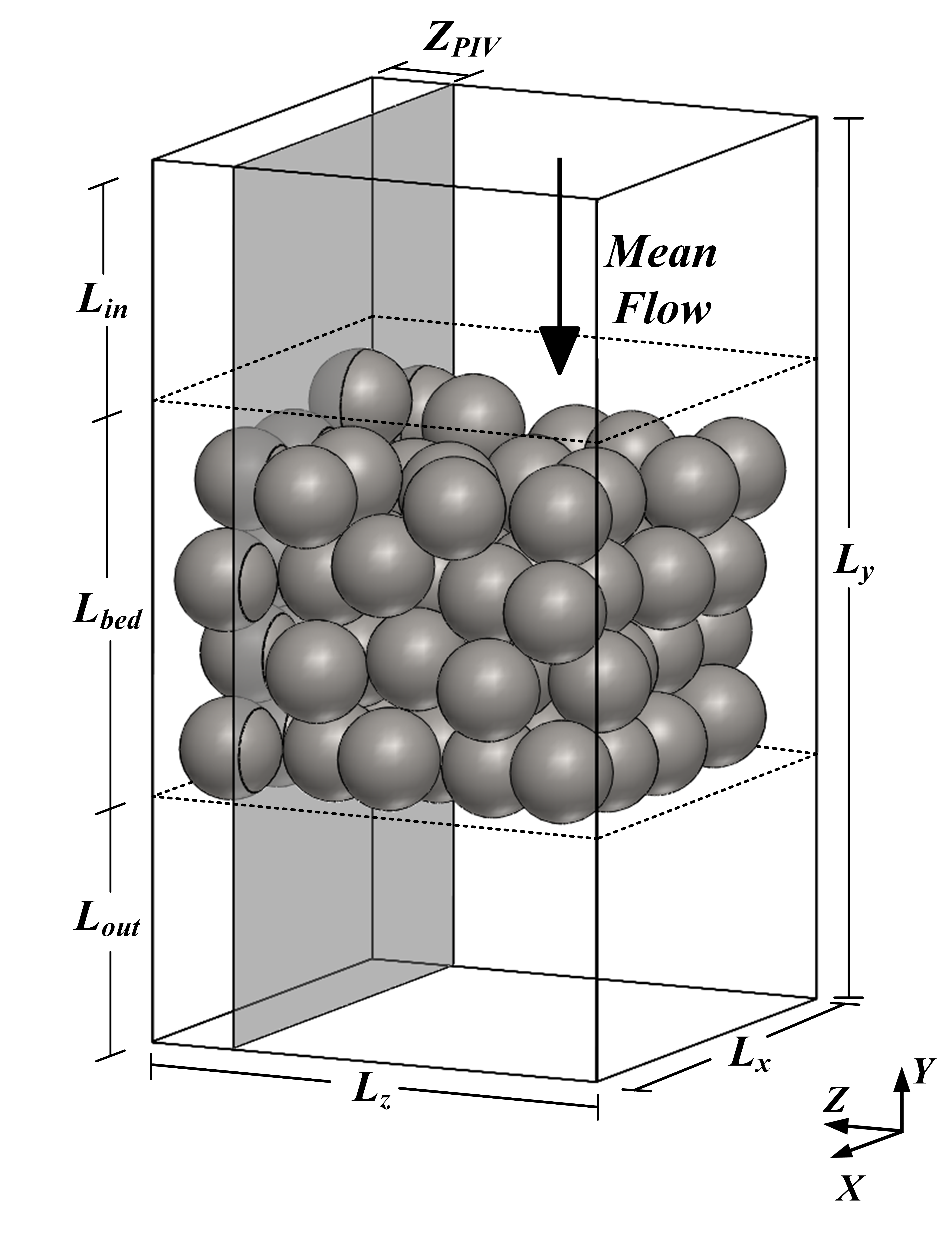
Figure 2: The three-dimensional geometry of the randomly packed porous bed. The location of one of the image planes for PIV data collection is shown for reference, image axis is along coordinate Z.

Refractive Index Matching (RIM) is required for optical imaging has been successful in a few studies [100, 101, 106, 114, 64, 70]. In the present work, high fidelity time-resolved PIV technique is used to measure the velocity field based on RIM. The results are used to address the following:

1. determination of the scaling of size, strength, and number density of the local vortical structures based on global and local pore scaling.

2. evaluation the dominant mechanisms, such as rotation or shear characteristics of vortices that influence the scale of the vortical structures in transition.

3. identification asymptotic limits for the size, strength, and number density of vortical structures in transition using local and global scaling.

This paper is organized as follows. In Section II, the details of geometry of the porous medium, flow-loop setup, measurement parameters, experimental method, and uncertainties are provided. Experimental results are presented in Section III with emphasis on the evolution of vortical structure size, scale, and number density during transition using vortex identification methods. In Section IV a summary discussion of the results together with conclusions are given.

II Methodology

The porous medium was designed for the collection of high-resolution velocity data with high quality images with low velocity uncertainty. In doing this the following elements were considered: (i) the geometry of porous system, (ii) refractive-index matching of porous medium, (iii) experimental setup detailing the method for collecting PIV velocity using RIM, and (iv) the uncertainty quantification for the PIV system.

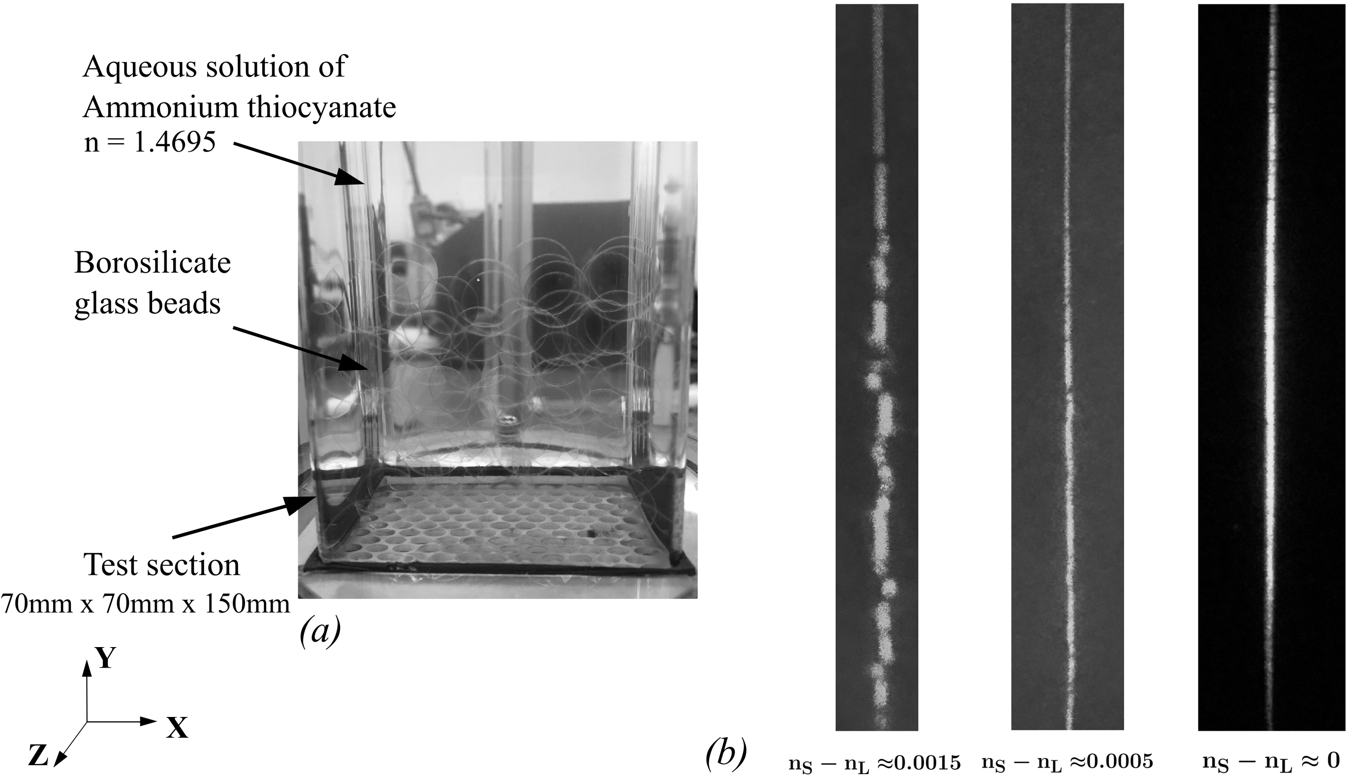
Figure 3: (a) Porous medium with solid and fluid phase refractive indices matched, (b) sequence of images of laser light sheet distortion when traveling through an index mismatched porous bed for light-sheet wavelength of $\lambda$ = 527 nm by applying these index mismatch values.

II.1 Geometry of porous medium

The random packed geometric arrangement is illustrated schematically in Figure 2. The plane of interest for PIV measurements is capable of being moved to any position along the optical axis (z-direction). The spherical beads, 15 $\rm mm$ diameter made from borosilicate glass, are optically homogeneous and transparent, with less than 0.01$\%$ uncertainty in their diameter. The mean flow convective velocity direction is from top to bottom in the negative Y-direction. Flow enters upstream of the porous bed through a channel with the same cross-section as the porous bed. Details of the test section, beads, and fluid are given in Table 1.

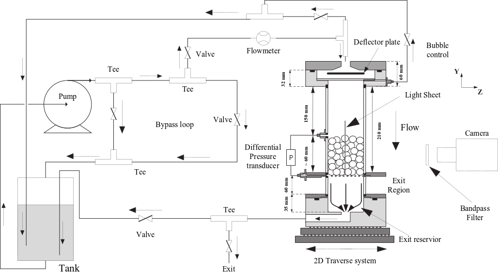
Figure 4: Schematic of the experimental flow loop and test section for PIV imaging together with the bubble control, and the bypass loop

II.2 Refractive-index matching

It is necessary to have an optically uniform porous bed for accurate RIM-PIV results [64, 101, 115, 116, 117, 118, 119, 120, 121, 122, 123]. The effect of even slight mismatches of refractive index has been evaluated using similar beads and fluid [64], with uncertainties associated with possible distortion presented in Section II.4. As a qualitative form of RIM distortion, Figure 3 (a) shows the porous bed with the random pack of glass spheres with refractive index of $\rm n_{S}=1.47$ that is matched with that of the fluid (aqueous solution of ammonium thiocyanate $\rm NH_{4}SCN$) with a refractive index of $\rm n_{L}=1.4695$. This corresponds to the middle laser sheet shown in Figure 3 (b), where there is a 0.03$\%$ mismatch with glass spheres. The laser sheet on the right shows no detectable mismatch between the solid and liquid, while the one on the left has 0.1 $\%$ of mismatch. In this study, the PIV imaging was obtained with the liquid refractive index within the range of $\rm 1.4695<n_{L}<1.47$ [64, 124, 118]. The liquid refractive index was measured using a referactometer (Atago co., Model: R5000).

Table 1: Experimental parameters used for the present study in the random porous bed.

Parameter	Symbol	Value
Porosity of porous media	$\Phi$	0.49
Bead Diameter  $\rm[mm]$	$\rm D_{B}$	$15$
Porous bed aspect ratio	$L_{x}/\rm D_{B}$	$4.67$
Inlet section length,  $\rm[mm]$	$L_{in}$	$155$
Outlet section length,  $\rm[mm]$	$L_{out}$	$60$
Porous medium length,  $\rm[mm]$	$L_{bed}$	$60$
Test section width, $x-$direction $\rm[mm]$	$L_{x}$	$70$
Test section width, $z-$direction $\rm[mm]$	$L_{z}$	$70$
Test section height, $y-$direction $\rm[mm]$	$L_{y}$	$270$
Apparatus glass wall refractive index (at $\lambda=527~{}\rm{nm}$)	$\rm n_{S}$	$1.47$
Glass Bead Refractive Index (at $\lambda=527~{}\rm{nm}$)	$\rm n_{S}$	$1.47$
Liquid Refractive Index (at $\lambda=527~{}\rm{nm}$)	$\rm n_{L}$	$1.4695\pm 0.0001$
Liquid Kinematic Viscosity $\rm[m^{2}/s]$	$\nu$	1.288 $\times$ $10^{-6}$
Liquid Density [$\rm Kg/m^{3}$]	$\rho$	1118
Tracer Diameter [$\rm\mu m$]	$D_{tracer}$	$10\pm 2$
Tracer Density [$\rm g/cm^{3}$]	$\rho_{tracer}$	$2.5\pm 0.1$
PIV conversion ratio	pixel/mm	18.207
PIV resolution [$vector/\rm D_{B}$]	$\rm\Delta_{PIV}$	$17.1$

II.3 Experimental setup

Two-dimensional PIV images in different x-y planes were taken in discrete locations along the z-direction, the optical axis, shown in Figure 2 using a traverse system of the test-section demonstrated schematically in Figure 4. The experimental flow loop (Figure 4) allows for a range of flow rates, and therefore Reynolds numbers. A total of 95 beads of 15 mm diameter, $D_{B}$, were used to create the porous bed. The packing was randomly set by the spheres into the square test section. The bed porosity, $\Phi$ was directly measured volumetrically to be 0.49, and the bed aspect ratio (width to bead diameter ratio) is 4.67.

The fluid density was 1118 $\rm kg/m^{3}$ and the tracer particles were manufactured by Dantec Dynamics, with a size of $10\pm 2\mu m$. The tracer particle response time was calculated to be much smaller than the Kolmogrov time scale [125], with a Stokes number $St_{tracer}=\rho_{tracer}D_{tracer}^{2}V_{int}/18\mu D_{B}\ll 1$, where $D_{tracer}$ is the tracer particle diameter and $\rho_{tracer}$ is the density of tracer particles.

Table 2: PIV configuration of different cases in the current study

Cases	$Z_{PL}/L_{z}$	$Re_{p}$	$\langle\overline{V}\rangle/V_{int}$	$\Phi_{PL}$
PL-1	0.5	100	0.82	0.45
PL-2	0.41	267	0.86	0.46
PL-3	0.4	272	0.88	0.49
PL-4	0.39	270	0.87	0.46
PL-5	0.3	253	0.81	0.41
PL-6	0.21	328-948	0.82-0.92	0.45

The imaging was based on high speed laser-pulsed lighting from a Nd-YLF laser (10000 Hz) at nominal wavelength of 527 nm (New Wave Research, Pegasus PIV). The camera was a CMOS (Integrated Design Tools Inc., Model: $\rm MotionPro^{TM}$X-3) with an adjustable focusing lens (Nikon AF Micro-NIKKOR 60mm f/2.8D). All data were gathered using an optimal f-number setting of 8 to compensate for both resolution and low uncertainty of in-plane motion. The imaging plane did not move relative to camera, hence, the magnification associated for each measuring plane was approximately constant, varying about 8$\%$ along the optical axis for the different planes; from 0.209 to 0.218. The interrogation window was $32\times 32$ pixels with 50$\%$ overlap to decrease noise. Thereby, the results are in a velocity vector spacing of 0.87 mm, equivalent to 17.1 vectors per bead diameter. Depending on the value of $Re_{p}$, the sampling frequency for each vector field ranged from 62 to 185 Hz corresponding to the lowest and highest $Re_{p}$, respectively. A total of 3200 velocity samples for each Reynolds number were captured. A high accuracy iterative adaptive PIV scheme specific to reducing out-of-plane loss of image pairs using $\rm Dantec\ Dynamics^{\circledR}$ was employed to perform image correlation, adaptive subpixel peak fitting, moving averaging, and subpixel deformation of the interrogation area. The validation process rejected less than $6.4\%$ of a total 4697 vectors as outliers.

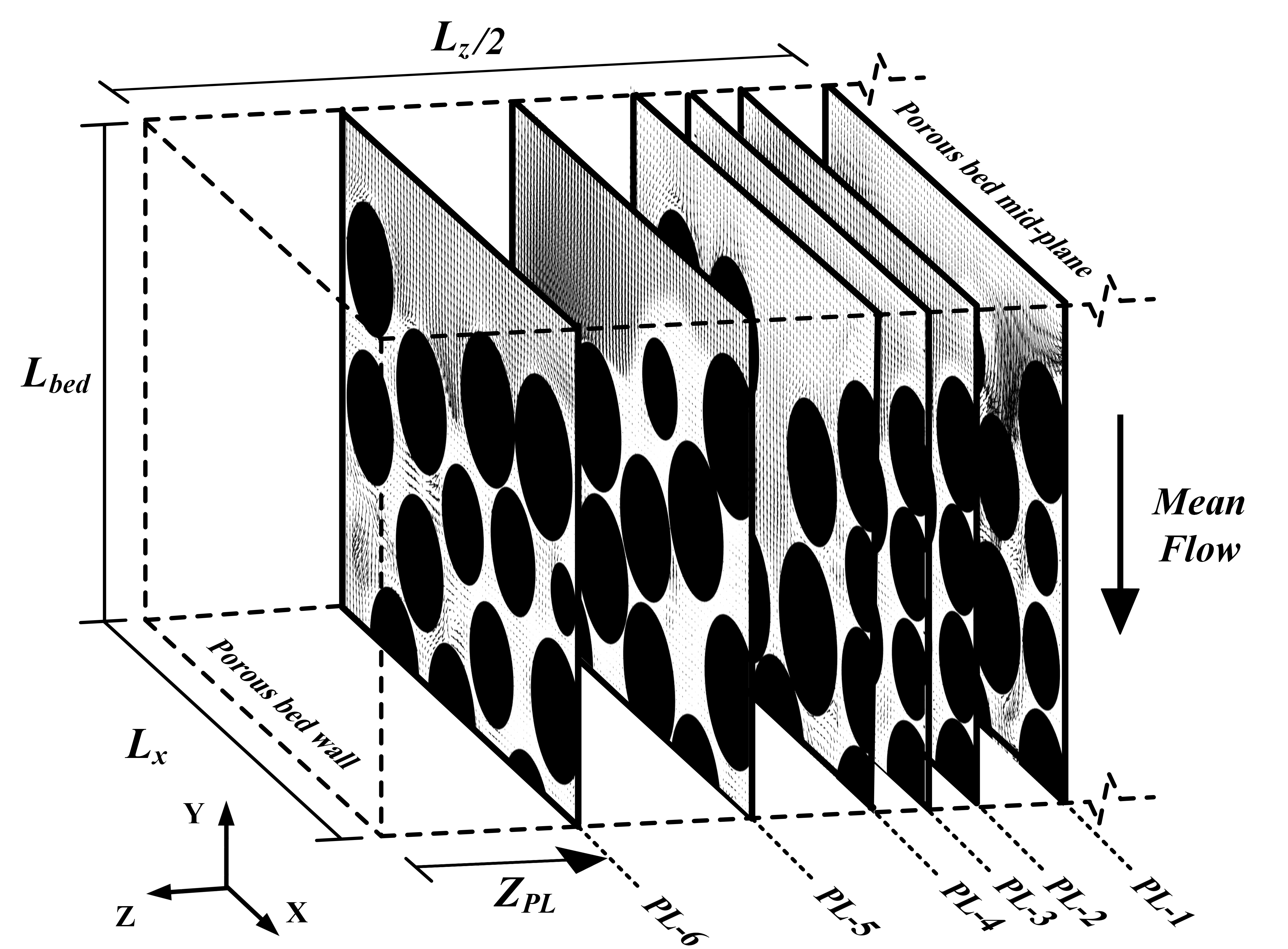
Figure 5: The vector-map configuration of instantaneous velocity at different planes in the experimental apparatus for Reynolds numbers ranging from 100 to 948. Six different test cases were obtained.

The data were obtained in six different planes along the optical axis (Z-direction) for the pore Reynolds numbers ranging from $Re_{p}=100$ to $Re_{p}=948$. Figure 5 is a schematic representation of six planes starting from the middle of the test-section (PL-1) towards the wall (PL-6). The plane closest to the wall was one bead length from the test-section wall. The details of the global conditions in each plane are summarized in Table 2. The size and shape of the pores in PL-2 to PL-4 are very similar with very nearly the same values of $Re_{p}$ of approximately 270. PL-6 is located within one bead diameter away from the wall and $Re_{p}$ ranged from 328-948. The geometry variations associated with plane PL-2 through PL-4 and their role on transition are also included.

Table 3: Uncertainty estimates for RIM porous media.

Uncertainty Source	$\varDelta$x [px]	$\varDelta$y [px]
Max displacement	4.45	8.69
In-plane loss of image pairs (bias)	0.091	0.091
Finite number of image pairs (random)	$\rm 0.037$	$0.037$
Refractive index mismatch error	$0.088$	$0.088$
Magnification	$0.07$	$0.012$
Displacement gradients	$0.011$	$0.056$
Out-of-plane motion (perspective)	$0.097$	$0.099$
Total error	$0.39$	0.4
Total error  [$\%$ of max displacement]	$8.8$	$4.6$

II.4 Uncertainty estimation

Comprehensive RIM-PIV uncertainty estimation is estimated based on six major sources of error addressed by Patil and Liburdy [64, 124, 49], Adrian and Westerweel[126], Raffel et al. [127], Northrup et al.[101], Sciacchitano et al. [128]. Uncertainty analysis was performed on all 3200 instantaneous PIV data collected for all six planes for $Re_{p}$ ranging from 100-948. Uncertainty sources are listed in Table 3. The light refraction uncertainties from the glass bead surfaces and test-section wall were minimized by using the optimal focal length and polarized laser sheet. The total uncertainty is quantified relative to the maximum displacement derived from the PL-6 velocity field. The maximum displacements in this experiment for the highest pore Reynolds number in the longitudinal or stream-wise direction (Y) is 8.69 pixels, while the lateral direction (X) experiences a maximum measured displacement of 4.45 pixels. The total error in the stream-wise direction (longitudinal) as a fraction of total y-displacement is 4.6$\%$, while it is 8.8$\%$ of maximum x-displacement in the cross-stream (lateral) direction.

The uncertainty associated with refractive-index mismatch is characterized by the method described in Patil and Liburdy [124], and the magnification error follows that described by Patil and Liburdy [64], while other sources were found based using typical PIV error estimations [128, 126, 127]. For estimating the in-plane loss of image pairs (bias error) as well as finite number of seed images in each interrogation window (random error), image shifting was used from 0 to 8 pixels with one pixel increments. The seed image displacement at the subpixel increments was applied based on interpolation using the nearest neighborhood. The total out-of-plane motion of particles were estimated to be 24$\%$ of the total error using the method given in (Ref.129). The velocity gradient error was determining by using central difference scheme [130, 126]. At the highest Reynolds number ($Re_{p}=948$), the velocity gradients uncertainty based on the propagation of random error is estimated to be 3.67 $s^{-1}$ which is 1.98$\%$ of max.

III Results and discussion

A detailed analysis on the scales associated with vortical structure characteristics is presented in this section. In summary, this section represents (i) the mean flow analysis with emphasis on flow structures (Section III.1), (ii) global scale estimation of vortical flow structures in different $Re_{p}$ (Section III.2), and (iii) local (pore-scale) scale estimation of vortical structures for the range of $Re_{\langle p\rangle}$ (Section III.3).

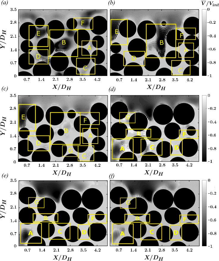
Figure 6: Contours of non-dimensional longitudinal velocity $\overline{V}/V_{int}$ overlayed with time-averaged normalized vector-map configuration of four different planes for Reynolds numbers ranging from 100 to 948; (a) Plane PL-1 at $Re_{p}=100$, (b) Plane PL-3 at $Re_{p}=272$, (c) Plane PL-4 at $Re_{p}=270$, (d) Plane PL-6 at $Re_{p}=528$, (e) Plane PL-6 at $Re_{p}=736$, and (f) Plane PL-6 at $Re_{p}=948$.

III.1 Mean Flow characteristics

Results of the mean velocity distribution are first presented to better understand the global effects of $Re_{p}$ within the entire bed. Referring to Figure 5, four planes of PL-1, PL-3, PL-4, and PL-6 were selected to study the variation of mean flow. The effect of Reynolds number ($Re_{p}$) and location of the plane relative to the bed was considered in studying the mean flow variations. The chosen planes were located in the middle of the bed (PL-1, PL-3, PL-4) and near the wall region (PL-6).

Shown in Figure 6, the variation of random geometrical arrangement of pores is a major contributor to have different distributions of mean velocity within the entire bed. Contours of time-averaged two-component velocity magnitude ($\overline{V}$) normalized by the interstitial velocity, $V_{int}$ are illustrated in Figure 6. The contours are overlayed with the normalized vector field demonstrating the local direction of the velocity at each specific pore. In this graph, local pores are indicated with rectangular regions representative of the area boundaries for selected regions to investigate the local flow structures. Selected pore-regions exhibit different flow characteristics in a heterogeneous pattern. The heterogeneity of the flow due to geometry has been observed by Johns et al. (2000) [35], and Sederman et al. (1998) [36] in the axial versus transverse directions, which is also discussed by Ogawa et al. (2000) [131] analogous to the axial variation of velocity magnitude shown in Figure 6. Furthermore, changes to the mean flow Reynolds number ($Re_{p}$) distributes the flow differently in each pore as shown in Figure 6. In addition to inertial effects, the viscous shear effects also contributes to the mean flow variations as it has been discussed by Hill and Koch (2001) [40] in a random packing structure. The pore-scale analysis discussed later in Section III.3 is based on the selected pores indicated in Figure 6.

The mean flow with a nearly uniform velocity profile enters the porous bed and accelerates or decelerates within the constriction regions in the interstices and becomes non-uniform depending on the pore-scale geometry causing the changes in pore-scale pressure, and velocity distribution. Therefore, a combination of different types of flow within these pores is created at different Reynolds numbers. The distribution of velocity is more homogeneous for $Re_{p}$ larger than 300, as shown in Figure 6.

Figure 6 (a) shows representative pores alphabetically ordered from A to F at a low Reynolds number of 100 (Plane PL-1). There are regions where flow behaves similar to a recirculation zone such as pore B, or a nozzle-like flow such as pore D. Also, in Figures 6 (a) and 6 (b), there are wake-like regions, as in pore B, where flow experiences a higher velocity. A wake extends behind the sphere in these pores on an order of 1-1.5$D_{H}$ and the flow accelerates downstream. However, in 6 (c), pore B represents a fairly uniform velocity distribution, which is not influenced by the wake region as opposed to planes PL-1 and PL-3 in Figures 6 (a), and 6 (b), respectively. Here, pore B is a three-dimensional void space that extends between PL-1 to PL-4, where the flow topology not only varies longitudinally but also the velocity distribution is affected in the transverse direction (z) as well. Figures 7 (a) to 7 (c) show the pore-scale contours of non-dimensional velocity magnitudes $\overline{V}/\langle\overline{V_{\langle P\rangle}}\rangle$ in pore B for PL-1, PL-3, and PL-4 mentioned above. The wake regions are magnified to show the pore-scale velocity distribution in pore B using three planes.

The PL-6 located nearer to the side walls, being 1.5 $D_{B}$ away from the wall. This plane has been shown in Figures 6 (d) to 6 (f) for three values of $Re_{p}$ of 528, 736, and 948. By increasing $Re_{p}$ the interestitial velocity also increases, hence the ratio of $\overline{V}/V_{int}$ becomes more homogeneous. There are two reasons for this: one, $Re_{p}$ has been increased such that the steady wake-like structures, or recirculation zones, are diminished by the mean flow inertia, and two, the porosity of PL-6 is smaller than the other planes, hence large flow patterns are damped due to higher geometrical confinements. Similar flow distribution effects has been reported by Hill et al. (2001)[40]. In PL-6, there are other pores that show other flow patterns such as a recirculation region shown in pore B in Figure 6 (d), where the flow occurs in a much smaller area, hence the recirculation is approximately 1/3$D_{B}$. Figures 7 (d) to 7 (e) also represent an expanded view of pore A in PL-6. The pore-scale contours of $\overline{V}/\langle\overline{V_{\langle P\rangle}}\rangle$ shows more homogeneity as $Re_{p}$ increases.

The local (pore-scale) length scale of the pores governs the flow structure sizes which is characterized by the local pore Reynolds number. These wake-like separated flows behind spheres have also been observed by Patil and Liburdy (2013) [49] at a pore Reynolds number of 418 with almost similar porosity, where the wake extends about 0.24$D_{H}$. On the other hand, Hill and Koch (2001) [40] simulated the wake structures in a dilute random array of spheres with higher porosity of 0.7 to 0.9. They hypothesized that the wake extends no further than an $O(\rm D_{B}/2(1-\phi))$ in moderate $Re_{p}\approx 300$ with $\phi\approx 0.75-0.9$. This is calculated to be in the order of $D_{H}$ in the present study, which is consistent with what is observed at $Re_{p}$ less than 300 in some pores. These wakes have also been observed in regular packing in numerical simulations. Chu et al. (2018) [42] reported such wake-like structures at a higher Reynolds number ($Re_{p}$ = 1000) with porosity of 0.75 in a regular array of square cylinders. He and Apte [72] investigated weak to strong wakes in a Face-Centred Cubic (FCC) array at pore Reynolds numbers 300, 500, and 1000 with low porosity of 0.26. They state that the wake-structure shows an organized (coherent) pattern which is due to the geometrical symmetry of the porous bed. However, as it is seen in Figure 6, the flow structures are artifacts of complex combination of flow inertia, and randomness of geometrical constrictions, as well as flow geometry heterogeneity. The porosity is another factor in the size of flow structures in porous media; larger wavelengths occur behind spheres in a high porosity bed.

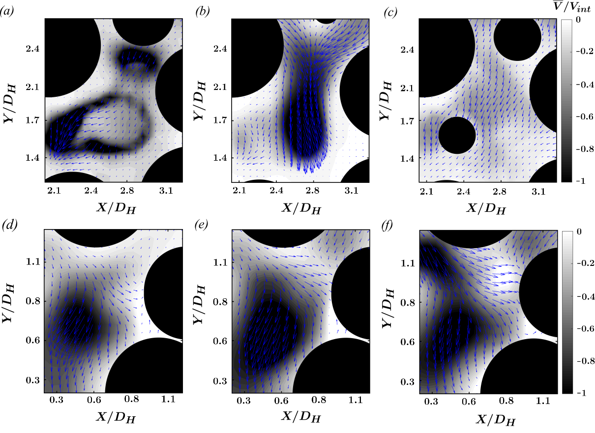
Figure 7: Pore-scale contours of non-dimensional longitudinal velocity $\overline{V}/\langle\overline{V_{\langle P\rangle}}\rangle$ overlayed with the time-averaged normalized vector-map of four planes for Reynolds numbers ranging from 100 to 948; (a) pore B in plane PL-1 at $Re_{p}=100$, (b) pore B in plane PL-3 at $Re_{p}=272$, (c) pore B in plane PL-4 at $Re_{p}=270$, (d) pore A in plane PL-6 at $Re_{p}=528$, (e) pore A in plane PL-6 at $Re_{p}=736$, and (f) pore A in plane PL-6 at $Re_{p}=948$.

High or low velocity regions in different pores are also the result of the tortuous three-dimensional flow in porous media. This feature is observed in Figure 7. Pore B (for PL-1, PL-3, and PL-4) shown in Figures 7 (a) to 7 (c), and Pore A for PL-6 shown in Figures 7 (d) to 7 (f) demonstrate high velocity pores that are results of the pore-scale out-of-plane motion of the flow in some specific pores within the bed. Moreover, the effect of spheres located outside of the plane of visualization sheds into the plane and a complex flow patterns is created with intermittent regions of high velocity as seen in pore B in Figure 7(a). As the plane of PIV moves closer to the wall, the normalized velocity in the porous bed exhibits a more uniform distribution in the entire plane.

III.2 Global scale of vortical flow structures

In this section, scales of the vortical structures for transitional flow are analyzed for the flow within the entire bed. Time-resolved PIV technique used in this study follows the Eulerian method of capturing velocity vectors instantaneously. Therefore, Eulerian vortex identification methods are used to detect the vortical structures. The swirl strength, known as point-wise (local) detection method of vortical structures ($\lambda_{ci}$, enhanced swirl strength ($\lambda_{cr}/\lambda_{ci}$) versus multiple-point (non-local) detection method of vortex core ($\varGamma_{2}$) are used [132, 133, 134]. Unique features of the evolution of vortical structures based on the integral length scale obtained from autocorrelation and also vortical size estimates derived from spatial distribution of vortex strength ($\lambda_{ci}$), vortex boundary ($\varGamma_{2}$), and size of spiral vortices ($\lambda_{cr}/\lambda_{ci}$). Also, strength of the vortex ($\lambda_{ci}$) as a vortex time-scale is compared with integral time-scales of the flow. Lastly, the number density of the vortical structures is found according to the number identified vortical structures based on $\lambda_{ci}$ criterion and the $\varGamma_{2}$ technique proposed by Michard et al. (1997) [135] and Graftieaux et al. (2001)[136].

The critical point analysis is based on the point-wise (local) linear approximation of the kinematics of local fluid motion at each point. Therefore, the local instantaneous velocity $\bm{V}$ around a point following the work proposed by Chong et al. (1990) [137] denoted by a position vector r can be expressed, to linear order, as [138, 139, 133]:

$$\bm{V}(\textit{r}+\delta\textit{r})=\bm{V}(\textit{r})+D_{ij}\ \delta\textit{r}+\textit{O}(\|\delta r\|^{2})$$ (3)

where, $D_{ij}=\nabla\bm{V}$ is the velocity gradient tensor with the characteristic equation of $D_{ij}$ is given by:

$$\lambda^{2}+P\lambda+R=0$$ (4)

where P and R are the two invariants of $D_{ij}$, which are defined as $P=\frac{\partial u}{\partial x}+\frac{\partial v}{\partial y}$, and $R=\frac{\partial u\partial v}{\partial x\partial y}+\frac{\partial u\partial v}{\partial y\partial x}$ where $u$ and $v$ are the $x$, and $y$ components of the velocity $\bm{V}$. By computing the imaginary component of the complex conjugate of the eigenvalue of the velocity gradient tensor, the field variable $\lambda_{ci}$ (local swirling strength) is determined for the flow[137, 133, 139]. This criterion is derived using a requirement, where the discriminant of characteristic equation becomes negative, then in this case, the discriminant has a conjugate pair of complex eigenvalues ($\lambda_{cr}\pm i\lambda_{ci}$).

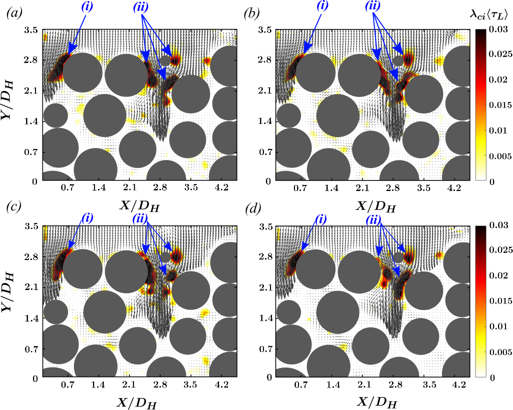
Figure 8: (a)-(d) Contours of the instantaneous swirl strength of detected vortical structures normalized by spatially averaged longitudinal Eulerian integral time scale ($\langle\tau_{L}\rangle$) overlayed on the LES filtered velocity with Gaussian kernel of $3\times 3$ plotted for $Re_{p}=270$ at four consecutive time intervals with the time-steps of $16.2\ ms$.

The condition through which vortical structures evolve with changing $Re_{p}$ differ due to topology of the pores, and local pore Reynolds number ($Re_{\langle p\rangle}$). To better observe the scale of flow structures, Large Eddy Scale (LES) filtering has been applied to the instantaneous velocity to separate the large scale flow structures from small scale vortices. A series of top-hat and Gaussian kernels have been convolved with each instantaneous velocity field [140]. A selected optimal kernel size for filtering based on $Re_{p}$ is performed. In laminar flow ($Re_{p}\leq 300$), a Gaussian filter with the kernel size of 5$\times$5 ($0.31D_{H}$) extracts the larger eddies from the unfiltered velocity, while for inertial and turbulent Reynolds numbers ($Re_{p}>300$), a Gaussian filter with a size of 3$\times$3 ($0.18D_{H}$) is used. In Figure 8, the contours of instantaneous $\lambda_{ci}$ are overlayed with LES filtered velocity using the Gaussian kernel of $3\times 3$.

In Figure 8, the global averaged Eulerian integral time scale for plane PL-4 ($Re_{p}=270$) is evaluated to be $\langle\tau_{L}\rangle=17.6~{}ms$ and the time interval between images is approximately $\langle\tau_{L}\rangle$. $\langle\tau_{L}\rangle$ is evaluated using the temporal autocorrelation of the longitudinal fluctuating velocity. The average vortex strength in this plane is 0.62 $s^{-1}$, showing that the frequency of the detected structures is much smaller than the sampling frequency for the data set. The dark regions of high $\lambda_{ci}$ near the surface of spheres shown by regions (i) and (ii) in Figure 8 are positioned similarly with almost identical cores in four consecutive time steps. These regions are consequences of high velocity gradients near the surface of spheres at a moderate $Re_{p}$ of approximately 300. They maintained their structures approximately within the time period shown in Figure 8, hence they are stretched but not broken up and carried with the mean flow inertia due to viscous effects near surfaces. The sequence shows distinct distortion over time as it is stretched by the mean flow. Speculated from the event shown in Figure 8, the vorticity develops nearly at distinct locations (due to highly tortuous bed structure) but with higher concentrations near the surface of spheres. These vortices are mostly stretched relative to the mean flow directions similar to the same behavior of vortices simulated in $Re_{p}=300$ for a regular packed bed [72].

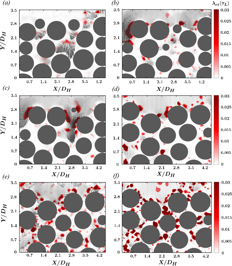
Figure 9: Contours of the instantaneous swirl strength of detected vortical structures normalized by the longitudinal Eulerian integral time scale ($\lambda_{ci}\tau_{L}$) overlayed on the LES filtered velocity with Gaussian kernel of $3\times 3$ plotted for a time step of $T=20\Delta\tau$ for all six cases of Figure 6. (a) Plane PL-1 at $Re_{p}=100$, (b) Plane PL-3 at $Re_{p}=272$, (c) Plane PL-4 at $Re_{p}=270$, (d) Plane PL-6 at $Re_{p}=528$, (e) Plane PL-6 at $Re_{p}=736$, and (f) Plane PL-6 at $Re_{p}=948$.

The results of evaluating the swirl strength, $\lambda_{ci}$, in six different planes of interest are given in Figure 9. The value of $\lambda_{ci}$ is normalized by the inverse of the bed averaged longitudinal integral time scale of the flow corresponding to each $Re_{p}$, $\langle\tau_{L}\rangle$. This set of figure shows the instantaneous vortical structures, and the location of vortical structures as they change while moving through the bed. However, for the lower Reynolds numbers (i.e $Re_{p}\leq 300$), many of the pore-scale structures are invariant in size and location; the uniform size of these steady coherent vortices develop near the surfaces as a consequence of shear dominated flows. Smaller rotational structures are weaker and are advected downstream. With increasing Reynolds number, these structures stretch, and break into smaller eddies as shown in Figures 9 (a) to 9 (f).

Analogous to high velocity gradient regions with large swirl strength ($\lambda_{ci}$) shown in Figure 8, the lower $Re_{p}$ conditions shown in Figure 9 (for cases with $Re_{p}$<300), contain vortical structures that are shear dominant as they tend to be generated near the surfaces of spheres in high velocity gradient regions. In higher $Re_{p}$ flows, these structures are advected downstream, where they are broken up to smaller eddies. To further reveal the regions with high velocity gradients, the instantaneous vorticity for pore B (which has a local high velocity) in PL-4 ($Re_{p}=270$) is discussed in Figure 10. The time history of four consecutive maps of non-dimensional out-of plane vorticity is illustrated for $Re_{p}=270$ (PL-4). The shear-dominant high vorticity regions are larger and have higher swirl strength (frequency) similar to regions (i), and (ii) in Figure 8. The generation of shear dominant vorticity near the surfaces and their elongation in the direction of mean flow have also been observed in other random packed beds such as (Ref. 141) at smaller $Re_{p}=150$ with $\phi=0.47$, as well as (Ref. 70) at larger $Re_{p}=340$ with porosity of 0.42. Comparing Figure 9 with Figure 10 illustrates the large areas of vorticity, where the $\lambda_{ci}$ criterion identifies the regions with intense vorticity and weakly detects the regions where the vorticity is in balance with strain rate [142].

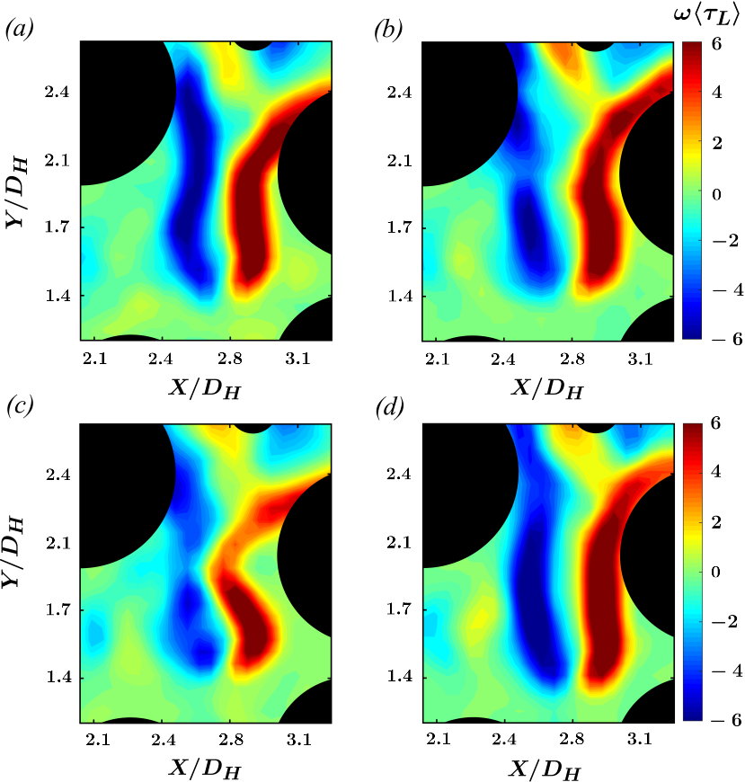
Figure 10: (a)-(d) Sequences of instantaneous out-of-plane vorticity contours of detected vortical structures normalized by spatially averaged inverse longitudinal Eulerian integral time scale ($\langle\tau_{L}\rangle$) plotted for $Re_{p}=270$ (PL-4) at four consecutive time steps with interval of 16.2 ms.

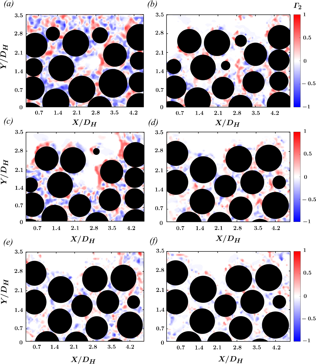
Figure 11: Instantaneous vortex core structures identified by $\Gamma_{2}$ scheme with a $3\times 3$ kernel size corresponding to 0.12$D_{B}$. (a) Plane PL-1 at $Re_{p}=100$, (b) Plane PL-3 at $Re_{p}=272$, (c) Plane PL-4 at $Re_{p}=270$, (d) Plane PL-6 at $Re_{p}=528$, (e) Plane PL-6 at $Re_{p}=736$, and (f) Plane PL-6 at $Re_{p}=948$. Computed values are for the whole porous bed.

Distinguishing between the rotational and shear dominant flow structures was employed by implementing $\varGamma_{2}$ function introduced by Graftieaux et al. (2001) [136], which is derived using velocity vector field directly. Thus, the $\varGamma_{2}$ criterion utilizes pseudo-circulation [132, 143] to identify vortex cores defined as:

$$\rm\varGamma_{2}(X;\textit{R})=\frac{1}{\pazocal{S}}\oint\limits_{X^{\prime}\in\pazocal{S}}\sin\theta\ \textit{d}X^{\prime}$$ (5)

where $\pazocal{S}$ is a disc surrounding point $\rm X$, $\rm X^{\prime}$ is any point surrounding point $\rm X$ in 2D PIV flow field within each $3\times 3$ subregion, $V$ is the velocity vector, $\sin\theta=|\delta X\times\delta V|/|\delta X||\delta V|$, $\delta X=X^{\prime}-X$, and $\delta V=V(X^{\prime})-\overline{V(X)}$, and $\overline{V(X)}$ is the average velocity evaluated in the subregion. The vortex core was then computed for eight vectors surrounding the point of interest in the flow field via $\varGamma_{2}=\frac{1}{8}\sum_{i=1}^{8}\sin\theta_{i}$. As a robust method that depends spatially on the velocities in a small neighborhood (non-local [132]), the subregion sweeps all over the vector field to detect vortex cores.

The vortical structures detected by the instantaneous $\varGamma_{2}$ criterion is given in Figure 11. The contours are color-coded based on the degree of fully rotational flow in the vortex center ($\lvert\varGamma_{2}\rvert=1$) versus the fully shear flow at the boundary of vortex ($\lvert\varGamma_{2}\rvert=0$). Therefore, a complete vortex zone is closer to 1, with positive sign representing counter-clockwise, while negative values describe clockwise flow [132, 144]. The shear dominant structures are identified when $\varGamma_{2}$ is less than $2/\pi$, while the rotational structures overcome the shear structures when $\varGamma_{2}\geq 2/\pi$ [136].

It is seen that in general, the size of the identified flow structures decreases with increasing $Re_{p}$. At $Re_{p}=100$ (Figure 11(a)), the flow is essentially laminar and flow structures are larger and dominated by shear, while the results for $Re_{p}=948$ (Figure 11(f)) displays relatively small distributed turbulent flow structures.

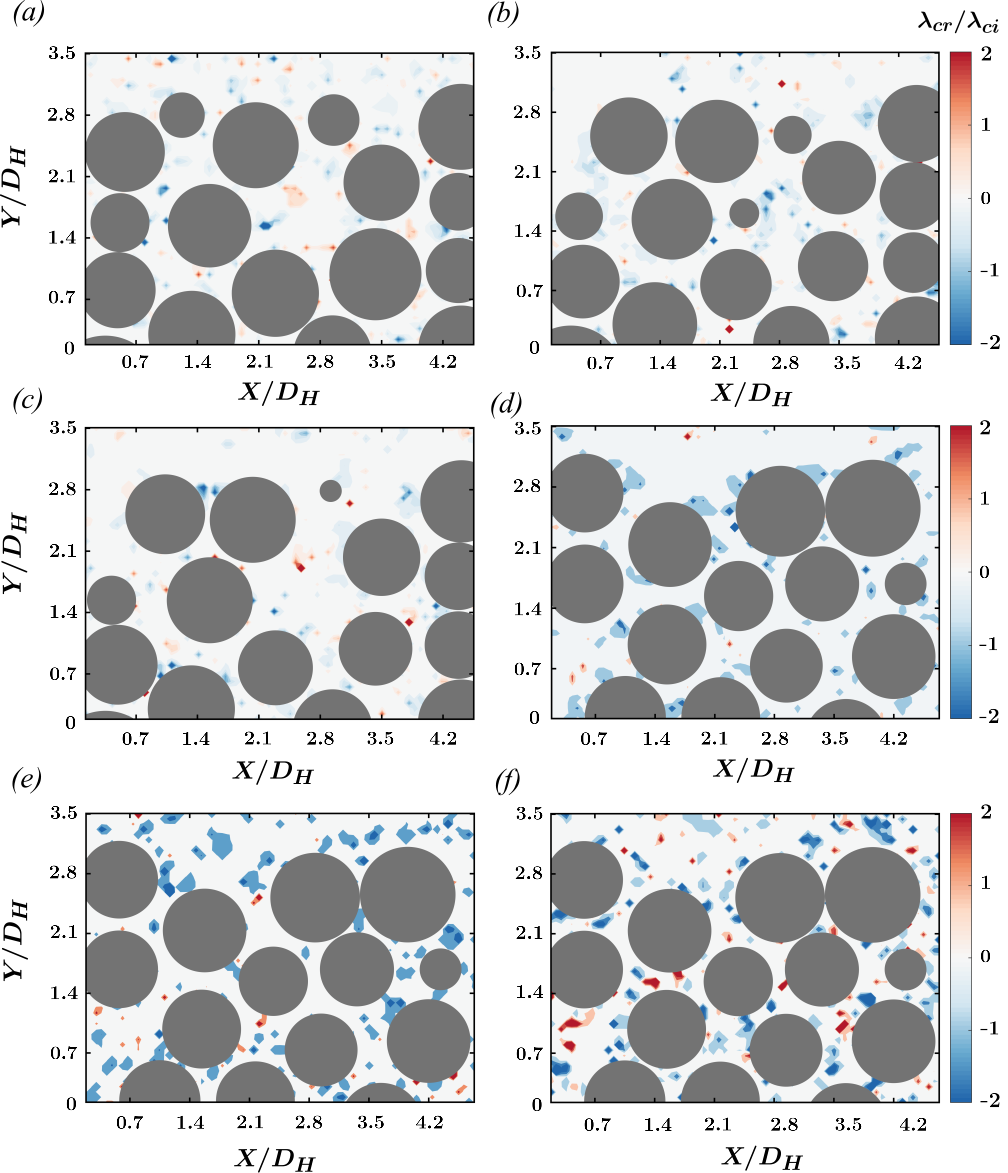
Figure 12: Instantaneous $\lambda_{cr}/\lambda_{ci}$ criterion indicating vortical structures with spiral motions passing through the plane of visualization at (a) Plane PL-1 at $Re_{p}=100$, (b) Plane PL-3 at $Re_{p}=272$, (c) Plane PL-4 at $Re_{p}=270$, (d) Plane PL-6 at $Re_{p}=528$, (e) Plane PL-6 at $Re_{p}=736$, and (f) Plane PL-6 at $Re_{p}=948$.

The $\lambda_{ci}$ criterion for vortex strength identification is Galilean invariant, which locally translates with the frame of reference[145]. The non-local identification of swirling structures [134] and their level of compactness or orbital shape is distinguished using $\lambda_{cr}/\lambda_{ci}$ (Chakraborty et al., 2005[145]). Using this method, the ability to detect the size of structures that are prone to elongate out of the plane of visualization is possible. Results are shown in Figure 12 for the size and number density of spiral vortices. It is obvious that the size, strength, and number density increases with $Re_{p}$. The number of spiral structures increases as they advect downstream in the y-direction due to the compactness of the pores, however, the size of the vortices are reduced. This is also observed based on $\lambda_{ci}$ (Figure 9), as well as $\varGamma_{2}$ (Figure 11). As stated by Chakraborty et al. (2005) [145], the presence of viscosity in real fluids results in the continuity of kinematics, which gives rise to the proximity of the estimates of vortical structures from $\lambda_{ci}$ as a local (pointwise, applied point by point) and the non-local method of $\varGamma_{2}$.

With increasing $Re_{p}$ shown in Figure 12, the size of detected vortices in the threshold of $-2\leq\lambda_{cr}/\lambda_{ci}\leq 2$ increases slightly in compliance with the three-dimensional tortuous effects of the porous media; thereby contributing to more spiral effects in vortical structures. The positive values of $\lambda_{cr}/\lambda_{ci}$ corresponds to outward spiraling motion of vortex, while negative values address the inward spirals. The areas where no vortex is detected based on $\lambda_{cr}/\lambda_{ci}$ corresponds to regions where there is no swirling in the flow since $\lambda_{ci}=0$. Thereby, the eigenvalue of $\nabla V$ does not have an imaginary pair in the regions with white color in Figure 12. The swirling spiral structures with intense out of plane motions are observed for $Re_{p}$ greater than 500.

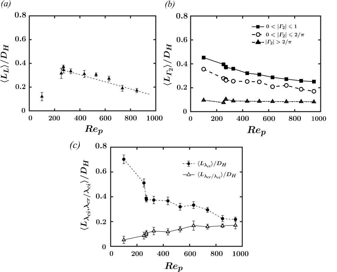
Figure 13: Vortex size in the entire porous bed: (a) the variations of vortex size computed based on longitudinal integral length scale ($\langle L_{L}\rangle$) normalized by $D_{H}$, (b) vortex size computed based on vortex boundary scheme ($\Gamma_{2}$) for the entire vortex core size ($\lvert\Gamma_{2}\rvert\leq 1$), shear-dominant votices ($\lvert\Gamma_{2}\rvert\leq 2/\pi$), and rotation-dominant vortices ($\lvert\Gamma_{2}\rvert\geq 2/\pi$), and (c) vortex size based on $\lambda_{ci}$ ($L_{\lambda_{ci}}$), as well as $\lambda_{cr}/\lambda_{ci}$ criteria. Computed values are scaled by hydraulic diameter $D_{H}$ for the whole porous bed for the cases of Reynolds numbers given in Table 2 .

The size of vortical structures is detected with the normalized Eulerian longitudinal integral length scale averaged over the entire porous bed for all six planes ($\langle L_{L}\rangle/D_{H}$) and is shown in Figure 13 (a) for the entire range of $Re_{p}$. The trend shows a decay of size with increasing $Re_{p}$ beyond 300. However, at $Re_{p}=100$ there is a reduced length scale ($\langle L_{L}\rangle/D_{H}$ = 0.12) since the has not transitioned to turbulence.

The $\varGamma_{2}$ vortex boundary method provides a means to predict the size of each vortex using these conditions: (i) $0<\varGamma_{2}\leq 1$, (ii) $0<\varGamma_{2}\leq 2/\pi$, and (iii) $\varGamma_{2}\geq 2/\pi$. The first describes all vortical structures (shear and rotational), while the second refers to shear dominated vortices, and the latter refers to the rotational structures with the condition of no vortex described by $\varGamma_{2}=0$. Similarly, the $\lambda_{ci}$ method also detects an area associated with each vortex based on a given threshold value. The size of each vortex was computed through image processing of the binarized image of detected vortices using both the $\varGamma_{2}$ vortex boundary method and swirl-strength criteria ($\lambda_{ci}$). Assuming a circular area for vortical structures, the diameter was found as a function of $Re_{p}$ which asymptotically converges to the value of 0.25$\rm D_{H}$ as shown in Figure 13 (b) along with the integral length scale. As shown, increasing $Re_{p}$ results in decreasing length scales with minimal changes for the rotational structures. Results seem to asymptote near $Re_{p}>800$ and are consistent with $\langle L_{L}\rangle/D_{H}$.

Figure 13 (c), exhibits the size of vortical structures detected based on $\lambda_{ci}$ [146, 133], as well as $\lambda_{cr}/\lambda_{ci}$ criteria normalized by $D_{H}$. The length scales are determined based on the thresholds of $0.001\leq\lambda_{ci}\leq 0.03$ and $0<\lvert\lambda_{cr}/\lambda_{ci}\rvert\leq 2$. The swirling structures show very large sizes ($L_{\lambda_{ci}}$) at $Re_{p}=100$ but then decrease to the results of the other methods discussed earlier. The size of spiralling structures ($L_{\lambda_{cr}/\lambda_{ci}}$) tend to increase with $Re_{p}$ and appears to reach an asymptotic length of $0.2D_{H}$ near $Re_{P}\sim 1000$ again consistent with the other measures. This trend is consistent with what has been observed in Figures 12 (a) to 12 (f) where the vortex core sizes of non-planar, orbital structures increases with $Re_{p}$. This slight increase can be speculated as the spiral structures are elongated at the pore-scale. Also, the concentration of these spiral structures is larger as $Re_{p}$ increases, where the vortices are closer to each other passing through the image plane of visualization in a time-frozen flow field. The same phenomena in a FCC case based on the helicity of vortical structures is observed during the transition from inertial to turbulent flow regimes [38, 72]. These results indicate that vortical sizes are constrained by, or scaled well, with the geometrical size of the pore. This feature is in agreement with Pore Scale Prevalence Hypothesis (PSPH) hypothesis [147, 148, 79], where the turbulent structures are postulated to exist within pore-scales and not beyond.

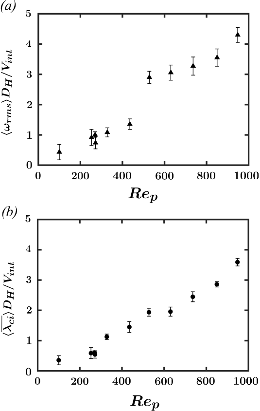
Figure 14: The variation of vortex strength versus $Re_{p}$ normalized by ($D_{H}/V_{int}$) (a) normalized vorticity rms $\langle\omega_{rms}\rangle D_{H}/V_{int}$, and (b) normalized time- and space-averaged vortex strength $\langle\overline{\lambda_{ci}}\rangle D_{H}/V_{int}$.

The spatio-temporal average of vortex strength is measured by both the rms vorticity and swirl strength, normalized by $D_{H}/V_{int}$ as shown in Figure 14 (where $V_{int}$ corresponds to each specific $Re_{p}$). The vorticity strength is seen to increase with $Re_{p}$ (Figure 14 (a)). Similarly, $\langle\overline{\lambda_{ci}}\rangle D_{H}/V_{int}$ shows an increasing trend with slightly lower values in Figure 14 (b). The asymptotic level of the strength of vortices based on the inverse of the pore-averaged integral time scale is found for $Re_{p}$ larger than 1000 is shown by Patil and Liburdy (2013) [49], to be $5.6V_{int}/D_{H}$. This value is fairly close with the value of strength found in the current study ($\sim 4-5V_{int}/D_{H}$).

The number of vortical structures identified increases with increasing the $Re_{p}$ as would be expected as shown in Figure 15 (a). These results are the temporal average of the number of vortical structures detected based on $\lambda_{ci}$ and $\varGamma_{2}$ within an imaging plane with a given planar porosity $\Phi_{PL}$ (given in Table 2). The results for the $\lambda_{ci}$ detection increase monotonically with $Re_{p}$ beyond $Re_{p}=300$. Results based on different Large Eddy Scale (LES) filter sizes show different values, based on a Gaussian filter size of 3$\times$3 ($0.18D_{H}$) versus 5$\times$5 ($0.31D_{H}$). The smaller filter represents scales above 0.18$D_{H}$ corresponding to the asymptotic results of length scales illustrated in Figure 13, which is approximately 0.2$D_{H}$. This indicates that the number of both small and larger scales are increasing with $Re_{p}$.

A spike is observed in Figure 15 (a) for $Re_{p}=267-270$ corresponding to PL-2, PL-3, and PL-4. These planes are located closely within the bed such that they share pores, and expectedly, vortical structures. PL-3 has higher $\Phi_{PL}$ (see Table 2) consistent with its larger average number of vortices compared with PL-2, and PL-4. The results based on $\varGamma_{2}$ detection (see Figure 15 (b)) are approximately the same order. Here, shear dominant ($\varGamma_{2}\leq 2/\pi$) and rotational dominant ($\varGamma_{2}\geq 2/\pi$) values are delineated. Interestingly, the shear dominant number decrease, while rotationally dominant ocurrances increase. This is consistent with the idea of smaller structures developing within the pores further from the boundaries. The shear dominant vortices are the highest when $Re_{p}\leq 300$.

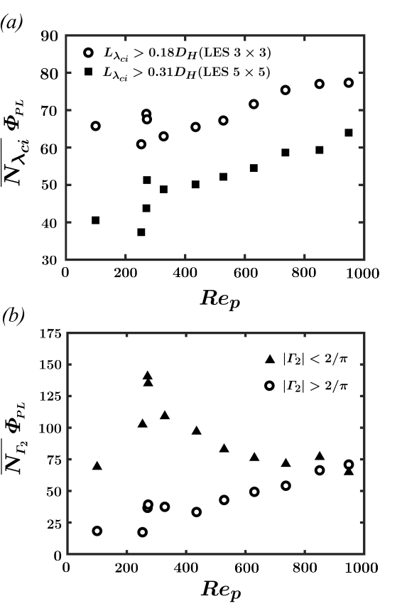
Figure 15: Temporal average of the number of detected vortical structures over all planes using (a) $\lambda_{ci}$ criterion with Gaussian filters for two kernel sizes of 3$\times$3 and 5$\times$5, and (b) $\Gamma_{2}$ for the shear-dominant votices ($\lvert\Gamma_{2}\rvert\leq 2/\pi$), and rotation-dominant vortices ($\lvert\Gamma_{2}\rvert\geq 2/\pi$).

III.3 Local scale of flow structures

Pore-level scale estimates of vortical structures for the range of pore-scale Reynolds numbers ($Re_{\langle p\rangle}$) defined in Section I are investigated in this section. These results emphasize local conditions and scaling. The local scales of the flow structures is based on each pore’s value of length scale and velocity scale. Results are presented for integral length scales, vortex size using $\lambda_{ci}$, $\varGamma_{2}$, local time-scales using vortex strength, and number density. The hydraulic diameter of individual pores ($D_{H_{\langle p\rangle}}$) is found from the following:

$$D_{H_{\langle p\rangle}}=\frac{4A_{\langle p\rangle}}{\mathscr{P_{\langle\it{p}\rangle}}}$$ (6)

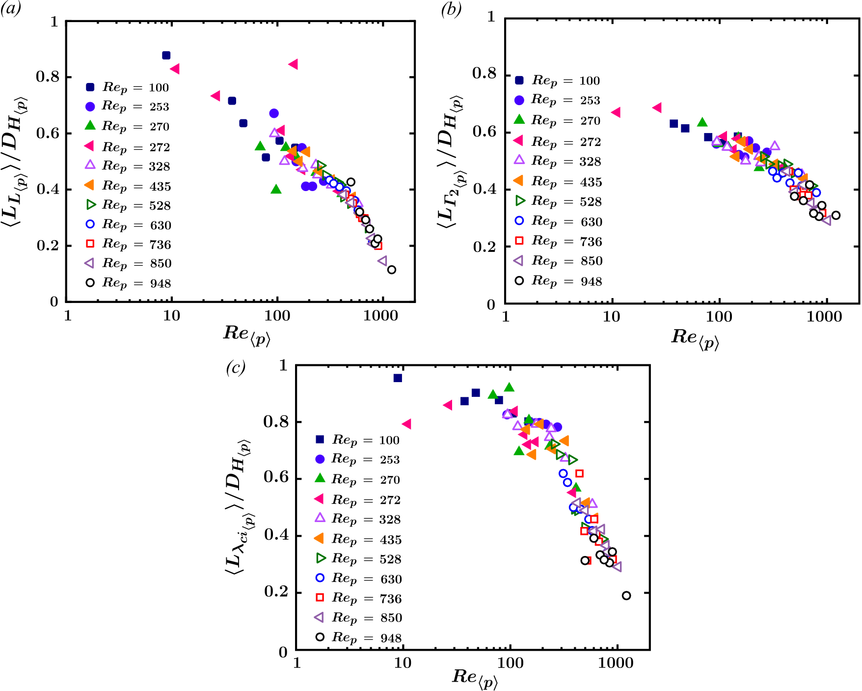
Figure 16: Variations of vortex size as a function microscopic Reynolds number ($Re_{\langle p\rangle}$) normalized by $D_{H_{\langle p\rangle}}$. (a) The variations of vortex size computed based on pore-averaged longitudinal integral length scale normalized by $D_{H}$, (b) vortex size computed based on vortex boundary scheme ($\Gamma_{2}$), and (c) vortex size based on $\lambda_{ci}$ ($L_{\lambda_{ci}}$) criteria.

where, $A_{\langle p\rangle}$ is the fluid area of an individual pore with boundaries indicated in Figure 6 (by excluding the solid areas of the beads), and $\mathscr{P_{\langle\it{p}\rangle}}$ is the wetted perimeter of the pore calculated by adding the solid boundary of pores (arc lengths of the pore walls) excluding the pore flow inlet and outlet areas.

In Figure 16, the overall size of vortical structures versus their corresponding $Re_{\langle p\rangle}$ is given. Figure 16 (a) is the pore-averaged longitudinal Eulerian integral length scale $\langle L_{L_{\langle p\rangle}}\rangle$ normalized by local pore-scale hydraulic diameter $D_{H_{\langle p\rangle}}$. Results show a decreasing trend with increasing $Re_{\langle p\rangle}$ on a log scale. For $Re_{\langle p\rangle}$ beyond approximately 100 data show a well-established and strong trend indicate that transition has occurred. Figure 16 (b) shows the length scales based on $\varGamma_{2}$ that also decreases very smoothly with $Re_{\langle p\rangle}$. Results found using $\lambda_{ci}$ is shown in Figure 16 (c), with a smaller trend as found for the other two methods but indicates a significantly greater rate of decay. These later results indicate larger structures at the lower values of $Re_{\langle p\rangle}$ but similar size of flow structures at the larger $Re_{\langle p\rangle}$ values. Given the wide variation of pore geometries and sizes as well as resultant $Re_{\langle p\rangle}$ values, these data show a well-established trend based on individual pore condition, but not the bed averaged results.

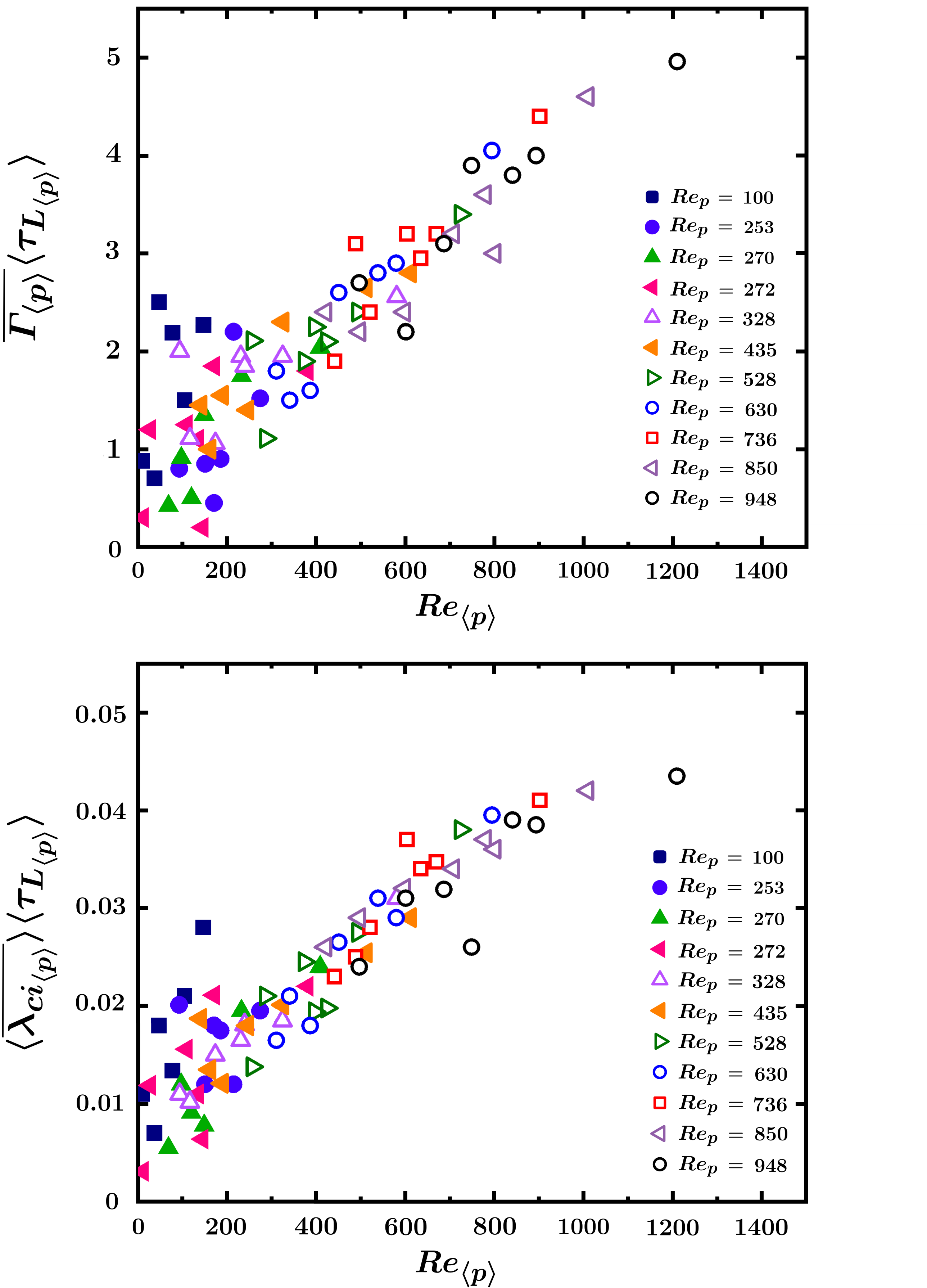
Figure 17: The variation of time averaged pore-scale vortex strength as a function pore-scale Reynolds number ($Re_{\langle p\rangle}$) non-dimensionalized by pore-averaged longitudinal time scale $\langle\tau_{L_{\langle p\rangle}}\rangle$. (a) Time averaged circulation $\overline{\varGamma_{\langle p\rangle}\langle}\tau_{L_{\langle p\rangle}}\rangle$, and (b) time and pore-averaged vortex strength $\langle\overline{\lambda_{ci_{\langle p\rangle}}}\rangle\langle\tau_{L_{\langle p\rangle}}\rangle$.

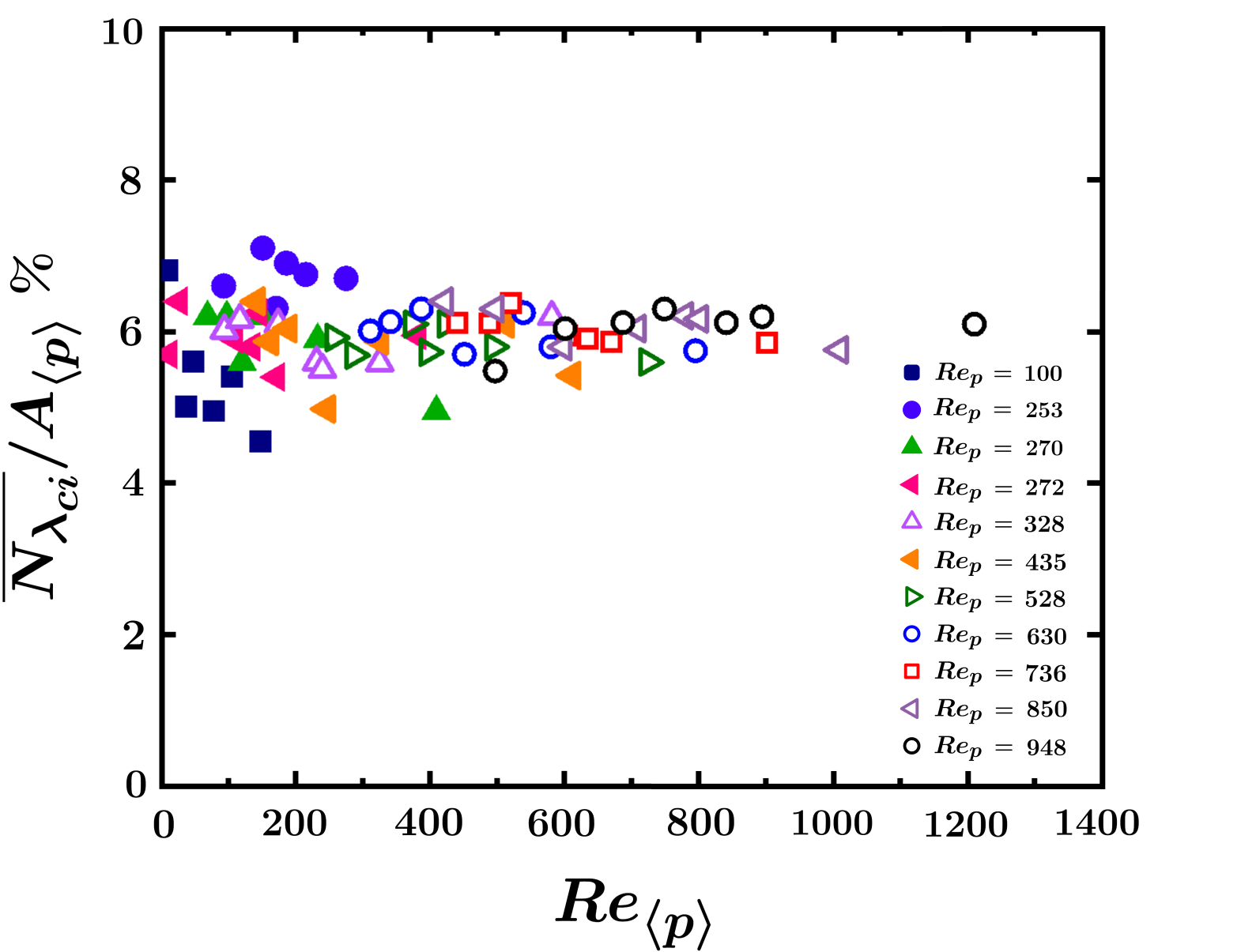
Figure 18: Temporal average of number of detected vortical structures in the entire bed based on $\lambda_{ci}$ criterion representing the number density of pore-scale vortical structures normalized by the area of pores ($A_{\langle p\rangle}$).

Figure 17(a) shows the non-dimensional strength of vortical structures evaluated for the range of local pore Reynolds numbers ($Re_{\langle p\rangle}$) using individual pore scaling. The total non-dimensional time-averaged circulation within a pore, and the is evaluated. The variation of circulation in each pore is dependent upon the pore-scale vorticity as plotted in Figure 17(a), where the circulation is calculated based on the sum of vorticity in each pore. The flow structures captured by circulation are originated from vorticity that included straining motions, pure shearing, and rotational structures [134]. The dominance of shear structures for low $Re_{\langle p\rangle}$ ($Re_{\langle p\rangle}$<300) contributes to an increase in variation of circulation, while the rotation is the major contributor for a larger circulation in higher $Re_{\langle p\rangle}$ ($Re_{\langle p\rangle}$ > 300). As flow transitions to turbulence, the value of $\overline{\varGamma_{\langle p\rangle}}\langle\tau_{L}\rangle$ is expected to increase with $Re_{\langle p\rangle}$ due to the larger vorticity created by velocity gradients in tortuous random pores. There is significant scatter for smaller $Re_{\langle p\rangle}$ ($Re_{\langle p\rangle}$ < 300), which is thought to be a result of transition to turbulence at the pore inflow conditions, and/or three dimensional effects. However, the trend shows less scatter at larger $Re_{\langle p\rangle}$s indicating pores with higher local vorticity. The pore-scale circulation of vortical structures follows a linear trend in $Re_{\langle p\rangle}>300$. For this range ($Re_{\langle p\rangle}>300$), the global $Re_{p}$ is also large indicative of transition in the vicinity of $Re_{\langle p\rangle}\approx 300$.

Figure 17(b), based on non-dimensional time- and pore-averaged vortex strength ($\overline{\lambda_{ci_{\langle p\rangle}}}\langle\tau_{L}\rangle$), illustrates the same trend as $\overline{\varGamma_{\langle p\rangle}}\langle\tau_{L}\rangle$. However, the rate of increasing $\overline{\lambda_{ci_{\langle p\rangle}}}\langle\tau_{L}\rangle$ are seen to be reduced after approximately $Re_{\langle p\rangle}>800$. This asymptotic trend is consistent with what has been observed by the number of vortical structures globally at $Re_{p}>800$ in Figure 15 (a), where the trends for both scales ($3\times 3$ and $5\times 5$) flattened. Unlike $\overline{\varGamma_{\langle p\rangle}}\langle\tau_{L}\rangle$, the variations of $\overline{\lambda_{ci_{\langle p\rangle}}}\langle\tau_{L}\rangle$ is lower at $Re_{\langle p\rangle}<300$.

The pore-scale variations of $\overline{\varGamma_{\langle p\rangle}}\langle\tau_{L}\rangle$ and $\overline{\lambda_{ci_{\langle p\rangle}}}\langle\tau_{L}\rangle$ shown in Figure 17 represent the consistent behavior of the pore-scale vortical structures analogous to the global strength of vortices shown in Figure 14. As a visual comparison, vorticity near the surface of spheres at lower $Re_{\langle p\rangle}$s are shear dominant with large strength due to the velocity gradient as shown by (i) and (ii) in Figure 8. Therefore, the variations of $\overline{\lambda_{ci_{\langle p\rangle}}}\langle\tau_{L}\rangle$ is mostly influenced by those shear dominated vortical structures. Similarly, strong vorticity regions at the inflow of a pore shown in Figure 10 is evidence of large variations of $\overline{\varGamma_{\langle p\rangle}}\langle\tau_{L}\rangle$ at low $Re_{\langle p\rangle}$s.

The percent of local time-averaged number of vortical structures normalized by the local pore area ($A_{\langle p\rangle}$) versus $Re_{\langle p\rangle}$ is shown in Figure 18. As shown, the ratio of number of vortical structures relative to the pore size is invariant with respect to $Re_{\langle p\rangle}$. The concentration of vortices are seen to be independent of the pore Reynolds number. Based on this, the overall number density of vortical structures is found to be a function of pore size. The number of detected vortices passing throughout each pore during the transition regime shows an invariance with respect to the size (area) of the pore. This seem to be the result of two possible features: pore-confinement, and the inertial effects. The level of confinement in random packed beds can control the possibility of pore-scale development of vortical structures. That is, pores with smaller sizes are reluctant to attract rotating structures from the mean flow and/or neighboring pores or they are small enough for the vortical structures to transport downstream. Moreover, pores with larger sizes are more prone to be influenced by the mean flow inertia that possibly increases the opportunity for the pore to develop shear effects. These conclusions are analogous to the geometry effects in high porosity random packed beds reported in simulations performed by Hill et al. (2001) [40]. Their findings shows the wavelengths of vortical flow structures (flow instabilities) are damped. Hence, vortical structures are less apt to be observed in highly confined pores.

IV Conclusion

High fidelity, time resolved particle image velocimetry were performed to identify vortical flow structures within a randomly packed porous media in six planes throughout the bed at global Reynolds numbers from 100 to 948. The effects of changing the Reynolds numbers as well as bed and pore geometry effects are investigated based on the vorticity distributions and vortical structures to evaluate size, strength (frequency), and number density using both macroscopic (global), and pore-scale (local) scales. Emphasis is placed on vortical structure scale evolution during transition and to scrutinize the use of the pore-scale Reynolds number to observe trends during transition in a random bed. The main observations are summarized below.

The mean flow influences the pore-scale flow due to tortuous characteristic of the random packing and generates wake-structures behind spheres, dead-zones, re-circulating vortical patterns, or elbow-like flows produced based on the geometry of pore, and flow acceleration, or deceleration of flow. These mean flow structures are observed not to exceed the limit of the local pore-level length scale orpore-scale hydraulic diameter ($D_{H_{\langle p\rangle}}$).

Vortical structures tend to demonstrate a steady behavior for lower values of $Re_{p}$ ($<300$). These quasi-steady flow structures are shear dominant and generated near the surfaces of spheres and enlarge to decelerate the mean flow. For larger values of $Re_{p}$ ($>300$), structures near the surface of spheres are broken up into smaller vortices that are advected downstream within pores.

Globally, the decay rate of the non-dimensional size of vortical structures versus the global $Re_{p}$ is similar to that observed when evaluated versus the pore-scale $Re_{\langle p\rangle}$. Some of these structures are rotational that tend not to vary in size with variation of $Re_{p}$, however, shear regions are shown to be reduced in size with increasing $Re_{p}$. The size of vortical structures using multiple techniques reach asymptotic values of $0.2-0.25D_{H}$ at $Re_{p}\sim 1000$. The level of compactness of vortical structures is reduced with increasing $Re_{p}$, hence, the size and number of vortical structures with spiral behavior is larger for $Re_{p}>500$. Locally, the size of vortical structures does not grow larger than the pore size or the global hydraulic diameter, hence it is in agreement with the PSPH hypothesis for the growth beyond the pore size. The dependence of integral length scale on the mean flow inertia is lower for small $Re_{\langle p\rangle}$. Additionally, larger variations occur of the size of vortices for $Re_{\langle p\rangle}<100$.

The vortex strength linearly increases with increasing $Re_{p}$. Locally, larger variations of strength are observed for low $Re_{\langle p\rangle}$. Moreover, the dominance of shear structures at lower $Re_{\langle p\rangle}$ contributes to an increase in the variation of circulation, however, the main reason for the increase in variation of circulation at larger $Re_{\langle p\rangle}$ is due to rotational vortices. Additionally, the pore-scale rate of growth in vortex strength is consistent with two different techniques implemented (i.e. $\overline{\varGamma_{\langle p\rangle}}$ and $\langle\overline{\lambda_{ci_{\langle p\rangle}}}\rangle$), but the variation of vortex strength for $Re_{\langle p\rangle}<300$ is slightly larger. It is speculated based on these observations, that the local geometry and confinement as well as three-dimensional flow in the pores have significant effect on the pore-scale strength of vortical structures.

Globally, the time-averaged number of vortical structures grows with increasing $Re_{p}$. Moreover, the total average number of vortical structures passing through each plane increases with the planar porosity. The shear dominant structures are reduced for increasing $Re_{p}$, whereas the rotational structures grow in number. Locally, it is shown that the larger the pore size, the more vortical structures are advected. Hence, the number of local vortices is seen to be influenced by the pore size during the transition.

The dependence of flow structures has been found to be correlated with the effects from local inertial in the flow which is in accordance with PSPH. Also, well-defined trends of transitional vortical scaling of size, strength and number density on individual pore has been observed. The scales are influenced by the pore geometry (size and curvature of interstices) of pores, and pore-scale Reynolds number. These results provide an alternate means to investigate the transition process particularly for random bed geometries. Findings of this study is an effort towards a better understanding of the evolution of the flow structures during transition in random packed beds.

References

- Gayev and Hunt [2007] Y. A. Gayev and J. C. Hunt, Flow and Transport Processes with Complex Obstructions: Applications to Cities, Vegetative Canopies and Industry, Vol. 236 (Springer Science & Business Media, 2007).
- Finnigan [2000] J. Finnigan, “Turbulence in plant canopies,” Annual review of fluid mechanics 32, 519–571 (2000).
- Dontsov [2016] E. Dontsov, “Tip region of a hydraulic fracture driven by a laminar-to-turbulent fluid flow,” Journal of Fluid Mechanics 797 (2016).
- Emerman, Turcotte, and Spence [1986] S. H. Emerman, D. Turcotte, and D. Spence, “Transport of magma and hydrothermal solutions by laminar and turbulent fluid fracture,” Physics of the earth and planetary interiors 41, 249–259 (1986).
- Tomac and Tartakovsky [2018] I. Tomac and D. M. Tartakovsky, “Experimental evaluation of turbulent flow and proppant transport in a narrow fracture,” in PROCEEDINGS, 43rd Workshop on Geothermal Reservoir Engineering, Stanford University, SGP-TR-213 (2018) pp. 1–9.
- Zolfaghari, Meyer, and Bunger [2017] N. Zolfaghari, C. R. Meyer, and A. P. Bunger, “Blade-shaped hydraulic fracture driven by a turbulent fluid in an impermeable rock,” Journal of Engineering Mechanics 143, 04017130 (2017).
- Geyer, Sarradj, and Fritzsche [2010] T. Geyer, E. Sarradj, and C. Fritzsche, “Measurement of the noise generation at the trailing edge of porous airfoils,” Experiments in Fluids 48, 291–308 (2010).
- Manes et al. [2009] C. Manes, D. Pokrajac, I. McEwan, and V. Nikora, “Turbulence structure of open channel flows over permeable and impermeable beds: A comparative study,” Physics of Fluids 21, 125109 (2009).
- Wu and Mirbod [2019] Z. Wu and P. Mirbod, “Instability analysis of the flow between two parallel plates where the bottom one coated with porous media,” Advances in Water Resources (2019).
- Rúa and Hernández [2016] D. Rúa and L. Hernández, “Phenomenological evaluation of industrial reformers for glycerol steam reforming,” International Journal of Hydrogen Energy 41, 13811–13819 (2016).
- Wehinger, Eppinger, and Kraume [2015] G. D. Wehinger, T. Eppinger, and M. Kraume, “Detailed numerical simulations of catalytic fixed-bed reactors: Heterogeneous dry reforming of methane,” Chemical Engineering Science 122, 197–209 (2015).
- Lucci et al. [2017] F. Lucci, A. Della Torre, G. Montenegro, R. Kaufmann, and P. D. Eggenschwiler, “Comparison of geometrical, momentum and mass transfer characteristics of real foams to kelvin cell lattices for catalyst applications,” International Journal of Heat and Mass Transfer 108, 341–350 (2017).
- Sharma, Cresswell, and Newson [1991] R. K. Sharma, D. L. Cresswell, and E. J. Newson, “Kinetics and fixed-bed reactor modeling of butane oxidation to maleic anhydride,” AIChE journal 37, 39–47 (1991).
- Latifi et al. [1989] M. Latifi, N. Midoux, A. Storck, and J. Gence, “The use of micro-electrodes in the study of the flow regimes in a packed bed reactor with single phase liquid flow,” Chemical engineering science 44, 2501–2508 (1989).
- Dave, Sun, and Hu [2018] A. Dave, K. Sun, and L. Hu, “Numerical simulations of molten salt pebble-bed lattices,” Annals of Nuclear Energy 112, 400–410 (2018).
- De Wasch and Froment [1972] A. De Wasch and G. Froment, “Heat transfer in packed beds,” Chemical Engineering Science 27, 567–576 (1972).
- Vadasz and Olek [1999] P. Vadasz and S. Olek, “Weak turbulence and chaos for low prandtl number gravity driven convection in porous media,” Transport in Porous Media 37, 69–91 (1999).
- Vadasz and Olek [2000] P. Vadasz and S. Olek, “Route to chaos for moderate prandtl number convection in a porous layer heated from below,” Transport in Porous Media 41, 211–239 (2000).
- Vadasz [2000] P. Vadasz, “Subcritical transitions to chaos and hysteresis in a fluid layer heated from below,” International Journal of Heat and Mass Transfer 43, 705–724 (2000).
- Vadasz [1999] P. Vadasz, “Local and global transitions to chaos and hysteresis in a porous layer heated from below,” Transport in Porous Media 37, 213–245 (1999).
- Vadasz [2015] P. Vadasz, “Feedback control for promoting or suppressing the transition to weak turbulence in porous media convection,” in Handbook of Porous Media, Third Edition, edited by K. Vafai (CRC Press, 2015) pp. 459–470.
- Howell, Hall, and Ellzey [1996] J. Howell, M. J. Hall, and J. L. Ellzey, “Combustion of hydrocarbon fuels within porous inert media,” Progress in Energy and Combustion Science 22, 121–145 (1996).
- Hall and Hiatt [1994] M. J. Hall and J. Hiatt, “Exit flows from highly porous media,” Physics of Fluids 6, 469–479 (1994).
- Lu et al. [2018] J. Lu, S. Das, E. Peters, and J. Kuipers, “Direct numerical simulation of fluid flow and mass transfer in dense fluid-particle systems with surface reactions,” Chemical Engineering Science 176, 1–18 (2018).
- Deen et al. [2012] N. G. Deen, S. H. Kriebitzsch, M. A. van der Hoef, and J. Kuipers, “Direct numerical simulation of flow and heat transfer in dense fluid–particle systems,” Chemical Engineering Science 81, 329–344 (2012).
- Deen et al. [2014] N. G. Deen, E. Peters, J. T. Padding, and J. Kuipers, “Review of direct numerical simulation of fluid–particle mass, momentum and heat transfer in dense gas–solid flows,” Chemical Engineering Science 116, 710–724 (2014).
- Khalili et al. [2010] A. Khalili, B. Liu, K. Javadi, M. R. Morad, K. Kindler, M. Matyka, R. Stocker, and Z. Koza, “Application of porous media theories in marine biological modeling,” in Porous Media: Applications in Biological Systems and Biotechnology (CRC Press, 2010) pp. 365–398.
- Khanafer et al. [2008] K. Khanafer, A. AlAmiri, I. Pop, and J. L. Bull, “Flow and heat transfer in biological tissues: application of porous media theory,” in Emerging Topics in Heat and Mass Transfer in Porous Media (Springer, 2008) pp. 237–259.
- Hlushkou and Tallarek [2006] D. Hlushkou and U. Tallarek, “Transition from creeping via viscous-inertial to turbulent flow in fixed beds,” Journal of Chromatography A 1126, 70–85 (2006).
- Hassanipour [2012] F. Hassanipour, “Analysis of vortex flow through porous media,” in AIP Conference Proceedings 4, Vol. 1453 (AIP, 2012) pp. 333–338.
- Hassanipour, Raya, and Mortazavi [2013] F. Hassanipour, I. P. Raya, and S. N. Mortazavi, “Simulation of vortex ring permeation in porous media,” Journal of Porous Media 16 (2013).
- Singh, Stoeber, and Green [2015] F. Singh, B. Stoeber, and S. I. Green, “Micro-piv measurement of flow upstream of papermaking forming fabrics,” Transport in Porous Media 107, 435–448 (2015).
- Larsson, Lundström, and Lycksam [2018] I. S. Larsson, T. S. Lundström, and H. Lycksam, “Tomographic piv of flow through ordered thin porous media,” Experiments in Fluids 59, 96 (2018).
- Suekane, Yokouchi, and Hirai [2003] T. Suekane, Y. Yokouchi, and S. Hirai, “Inertial flow structures in a simple-packed bed of spheres,” AIChE journal 49, 10–17 (2003).
- Johns et al. [2000] M. Johns, A. Sederman, A. Bramley, L. Gladden, and P. Alexander, “Local transitions in flow phenomena through packed beds identified by mri,” AIChE journal 46, 2151–2161 (2000).
- Sederman et al. [1998] A. Sederman, M. Johns, P. Alexander, and L. Gladden, “Structure-flow correlations in packed beds,” Chemical Engineering Science 53, 2117–2128 (1998).
- Hill and Koch [2002a] R. J. Hill and D. L. Koch, “Moderate-reynolds-number flow in a wall-bounded porous medium,” Journal of Fluid Mechanics 453, 315–344 (2002a).
- Hill and Koch [2002b] R. J. Hill and D. L. Koch, “The transition from steady to weakly turbulent flow in a close-packed ordered array of spheres,” Journal of Fluid Mechanics 465, 59–97 (2002b).
- Soulaine et al. [2017] C. Soulaine, M. Quintard, B. Baudouy, and R. Van Weelderen, “Numerical investigation of thermal counterflow of he ii past cylinders,” Physical review letters 118, 074506 (2017).
- Hill, Koch, and Ladd [2001] R. J. Hill, D. L. Koch, and A. J. Ladd, “Moderate-reynolds-number flows in ordered and random arrays of spheres,” Journal of Fluid Mechanics 448, 243–278 (2001).
- Koch and Hill [2001] D. L. Koch and R. J. Hill, “Inertial effects in suspension and porous-media flows,” Annual Review of Fluid Mechanics 33, 619–647 (2001).
- Chu, Weigand, and Vaikuntanathan [2018] X. Chu, B. Weigand, and V. Vaikuntanathan, “Flow turbulence topology in regular porous media: From macroscopic to microscopic scale with direct numerical simulation,” Physics of Fluids 30, 065102 (2018).
- Sahimi [2011] M. Sahimi, “Characterization of the morphology of porous media,” in Flow and Transport in Porous Media and Fractured Rock, edited by M. Sahimi (John Wiley Sons, 2011) Chap. 4, pp. 39–108.
- Stoop et al. [2019] N. Stoop, N. Waisbord, V. Kantsler, V. Heinonen, J. S. Guasto, and J. Dunkel, “Disorder-induced topological transition in porous media flow networks,” Journal of Non-Newtonian Fluid Mechanics 268, 66–74 (2019).
- Anna et al. [2013] P. d. Anna, J. Jimenez-Martinez, H. Tabuteau, R. Turuban, T. Le Borgne, M. Derrien, and Y. Meheust, “Mixing and reaction kinetics in porous media: An experimental pore scale quantification,” Environmental science technology 48, 508–516 (2013).
- Dullien [1991] F. A. Dullien, Porous media: fluid transport and pore structure (Academic press, 1991).
- Shimizu and Tanaka [2017] R. Shimizu and H. Tanaka, “Impact of complex topology of porous media on phase separation of binary mixtures,” Science advances 3, eaap9570 (2017).
- Vogel [2002] H.-J. Vogel, “Topological characterization of porous media,” in Morphology of condensed matter (Springer, 2002) pp. 75–92.
- Patil and Liburdy [2013a] V. A. Patil and J. A. Liburdy, “Turbulent flow characteristics in a randomly packed porous bed based on particle image velocimetry measurements,” Physics of Fluids 25, 043304 (2013a).
- Wu, Ma, and Zhou [2007] J.-Z. Wu, H.-Y. Ma, and M.-D. Zhou, Vorticity and vortex dynamics (Springer Science & Business Media, 2007).
- Scheidegger [1958] A. Scheidegger, The physics of flow through porous media (University Of Toronto Press: London, 1958).
- Bear [1972] J. Bear, Dynamics of fluids in porous media (American Elsevier, 1972).
- Wood, He, and Apte [2020] B. D. Wood, X. He, and S. V. Apte, “Modeling turbulent flows in porous media,” Annual Review of Fluid Mechanics 52 (2020).
- Jolls and Hanratty [1966] K. Jolls and T. Hanratty, “Transition to turbulence for flow through a dumped bed of spheres,” Chemical Engineering Science 21, 1185–1190 (1966).
- Ward [1964] J. Ward, “Turbulent flow in porous media,” Journal of the Hydraulics Division 90, 1–12 (1964).
- Wright [1968] D. E. Wright, “Nonlinear flow through granular media,” Journal of the Hydraulics Division 94, 851–872 (1968).
- Wegner, Karabelas, and Hanratty [1971] T. H. Wegner, A. J. Karabelas, and T. J. Hanratty, “Visual studies of flow in a regular array of spheres,” Chemical Engineering Science 26, 59–63 (1971).
- Karabelas, Wegner, and Hanratty [1971] A. J. Karabelas, T. H. Wegner, and T. J. Hanratty, “Use of asymptotic relations to correlate mass transfer data in packed beds,” Chemical Engineering Science 26, 1581–1589 (1971).
- Dybbs and Edwards [1984] A. Dybbs and R. Edwards, “A new look at porous media fluid mechanics—darcy to turbulent,” in Fundamentals of transport phenomena in porous media (Springer, 1984) pp. 199–256.
- Seguin et al. [1998] D. Seguin, A. Montillet, J. Comiti, and F. Huet, “Experimental characterization of flow regimes in various porous media—ii: Transition to turbulent regime,” Chemical engineering science 53, 3897–3909 (1998).
- Seguin, Montillet, and Comiti [1998] D. Seguin, A. Montillet, and J. Comiti, “Experimental characterisation of flow regimes in various porous media—i: Limit of laminar flow regime,” Chemical engineering science 53, 3751–3761 (1998).
- Bu et al. [2014] S. Bu, J. Yang, Q. Dong, and Q. Wang, “Experimental study of transition flow in packed beds of spheres with different particle sizes based on electrochemical microelectrodes measurement,” Applied Thermal Engineering 73, 1525–1532 (2014).
- Thaker, Karthik, and Buwa [2019] A. H. Thaker, G. Karthik, and V. V. Buwa, “Piv measurements and cfd simulations of the particle-scale flow distribution in a packed bed,” Chemical Engineering Journal 374, 189–200 (2019).
- Patil and Liburdy [2012] V. A. Patil and J. A. Liburdy, “Optical measurement uncertainties due to refractive index mismatch for flow in porous media,” Experiments in fluids 53, 1453–1468 (2012).
- Patil and Liburdy [2015] V. A. Patil and J. A. Liburdy, “Scale estimation for turbulent flows in porous media,” Chemical Engineering Science 123, 231–235 (2015).
- Hellstrom, Jonsson, and Lundstrom [2010] J. G. I. Hellstrom, P. J. P. Jonsson, and T. S. Lundstrom, “Laminar and turbulent flowthrough an array of cylinders,” Journal of Porous Media 13 (2010).
- Finn and Apte [2013] J. Finn and S. V. Apte, “Relative performance of body fitted and fictitious domain simulations of flow through fixed packed beds of spheres,” International Journal of Multiphase Flow 56, 54–71 (2013).
- Wood et al. [2015] B. Wood, S. Apte, J. Liburdy, R. Ziazi, X. He, J. Finn, and V. Patil, “A comparison of measured and modeled velocity fields for a laminar flow in a porous medium,” Advances in water resources 85, 45–63 (2015).
- Khayamyan et al. [2017] S. Khayamyan, T. S. Lundström, J. G. I. Hellström, P. Gren, and H. Lycksam, “Measurements of transitional and turbulent flow in a randomly packed bed of spheres with particle image velocimetry,” Transport in Porous Media 116, 413–431 (2017).
- Nguyen et al. [2018] T. Nguyen, E. Kappes, S. King, Y. Hassan, and V. Ugaz, “Time-resolved piv measurements in a low-aspect ratio facility of randomly packed spheres and flow analysis using modal decomposition,” Experiments in Fluids 59, 127 (2018).
- He et al. [2018] X. He, S. Apte, K. Schneider, and B. Kadoch, “Angular multiscale statistics of turbulence in a porous bed,” Physical Review Fluids 3, 084501 (2018).
- He et al. [2019] X. He, S. V. Apte, J. R. Finn, and B. D. Wood, “Characteristics of turbulence in a face-centred cubic porous unit cell,” Journal of Fluid Mechanics 873, 608–645 (2019).
- Nguyen et al. [2019] T. Nguyen, R. Muyshondt, Y. Hassan, and N. Anand, “Experimental investigation of cross flow mixing in a randomly packed bed and streamwise vortex characteristics using particle image velocimetry and proper orthogonal decomposition analysis,” Physics of Fluids 31, 025101 (2019).
- Kececioglu and Jiang [1994] I. Kececioglu and Y. Jiang, “Flow through porous media of packed spheres saturated with water,” Journal of Fluids Engineering 116, 164–170 (1994).
- Kaviany [1992] M. Kaviany, Principles of heat transfer in porous media (Springer Science & Business Media, 1992).
- Reynolds, Reavell, and Harral [2000] A. Reynolds, S. Reavell, and B. Harral, “Flow and dispersion through a close-packed fixed bed of spheres,” Physical Review E 62, 3632 (2000).
- Horton and Pokrajac [2009] N. Horton and D. Pokrajac, “Onset of turbulence in a regular porous medium: An experimental study,” Physics of fluids 21, 045104 (2009).
- Agnaou, Lasseux, and Ahmadi [2016] M. Agnaou, D. Lasseux, and A. Ahmadi, “From steady to unsteady laminar flow in model porous structures: an investigation of the first hopf bifurcation,” Computers & Fluids 136, 67–82 (2016).
- Jin et al. [2015] Y. Jin, M.-F. Uth, A. Kuznetsov, and H. Herwig, “Numerical investigation of the possibility of macroscopic turbulence in porous media: a direct numerical simulation study,” Journal of Fluid Mechanics 766, 76–103 (2015).
- Nakamura [1976] I. Nakamura, “Steady wake behind a sphere,” The Physics of Fluids 19, 5–8 (1976).
- Natarajan and Acrivos [1993] R. Natarajan and A. Acrivos, “The instability of the steady flow past spheres and disks,” Journal of Fluid Mechanics 254, 323–344 (1993).
- Taneda [1956] S. Taneda, “Experimental investigation of the wake behind a sphere at low reynolds numbers,” Journal of the Physical Society of Japan 11, 1104–1108 (1956).
- Goldburg and Florsheim [1966] A. Goldburg and B. Florsheim, “Transition and strouhal number for the incompressible wake of various bodies,” The Physics of Fluids 9, 45–50 (1966).
- Kim and Pearlstein [1990] I. Kim and A. J. Pearlstein, “Stability of the flow past a sphere,” Journal of Fluid Mechanics 211, 73–93 (1990).
- Johnson and Patel [1999] T. Johnson and V. Patel, “Flow past a sphere up to a reynolds number of 300,” Journal of Fluid Mechanics 378, 19–70 (1999).
- Gumowski et al. [2008] K. Gumowski, J. Miedzik, S. Goujon-Durand, P. Jenffer, and J. Wesfreid, “Transition to a time-dependent state of fluid flow in the wake of a sphere,” Physical Review E 77, 055308 (2008).
- Szaltys et al. [2012] P. Szaltys, M. Chrust, A. Przadka, S. Goujon-Durand, L. Tuckerman, and J. Wesfreid, “Nonlinear evolution of instabilities behind spheres and disks,” Journal of Fluids and Structures 28, 483–487 (2012).
- Skarysz et al. [2018] M. Skarysz, J. Rokicki, S. Goujon-Durand, and J. E. Wesfreid, “Experimental investigation of the wake behind a rotating sphere,” Physical Review Fluids 3, 013905 (2018).
- Ergun [1952] S. Ergun, “Fluid flow through packed columns,” Chem. Eng. Prog. 48, 89–94 (1952).
- Dudgeon [1966] C. Dudgeon, “An experimental study of the flow of water through coarse granular media,” La Houille Blanche 7, 785–801 (1966).
- Kyle and Perrine [1971] C. R. Kyle and R. Perrine, “An experimental model for visual studies of turbulent flow in porous materials,” The Canadian Journal of Chemical Engineering 49, 19–24 (1971).
- Fand et al. [1987] R. Fand, B. Kim, A. Lam, and R. Phan, “Resistance to the flow of fluids through simple and complex porous media whose matrices are composed of randomly packed spheres,” Journal of fluids engineering 109, 268–273 (1987).
- Mickley, Smith, and Korchak [1965] H. Mickley, K. Smith, and E. Korchak, “Fluid flow in packed beds,” Chemical Engineering Science 20, 237–246 (1965).
- Rode et al. [1994] S. Rode, N. Midoux, M. Latifi, A. Storck, and E. Saatdjian, “Hydrodynamics of liquid flow in packed beds: an experimental study using electrochemical shear rate sensors,” Chemical Engineering Science 49, 889–900 (1994).
- Lahbabi and Chang [1985] A. Lahbabi and H.-C. Chang, “High reynolds number flow through cubic arrays of spheres steady-state solution and transition to turbulence,” Chemical engineering science 40, 435–447 (1985).
- Masuoka, Takatsu, and Inoue [2003] T. Masuoka, Y. Takatsu, and T. Inoue, “Chaotic behavior and transition to turbulence in porous media,” Microscale Thermophysical Engineering 6, 347–357 (2003).
- Fourar et al. [2004] M. Fourar, G. Radilla, R. Lenormand, and C. Moyne, “On the non-linear behavior of a laminar single-phase flow through two and three-dimensional porous media,” Advances in Water resources 27, 669–677 (2004).
- Takatsu and Masuoka [2005] Y. Takatsu and T. Masuoka, “Transition process to turbulent flow in porous media,” in ASME 2005 International Mechanical Engineering Congress and Exposition (American Society of Mechanical Engineers, 2005) pp. 573–578.
- Jost [2018] A. M. D. Jost, Direct Numerical Simulations of Incompressible Flow through Porous Packs over a wide Range of Reynolds Numbers, Ph.D. thesis, Florida Institute of Technology (2018).
- Saleh, Thovert, and Adler [1992] S. Saleh, J. Thovert, and P. Adler, “Measurement of two-dimensional velocity fields in porous media by particle image displacement velocimetry,” Experiments in Fluids 12, 210–212 (1992).
- Northrup et al. [1993] M. A. Northrup, T. J. Kulp, S. M. Angel, and G. F. Pinder, “Direct measurement of interstitial velocity field variations in a porous medium using fluorescent-particle image velocimetry,” Chemical Engineering Science 48, 13–21 (1993).
- Patil et al. [2014] V. Patil, J. Finn, X. He, R. Ziazi, S. V. Apte, J. A. Liburdy, and B. Wood, “Experimental versus computational methods in the study of flow in porous media,” in ASME 2014 4th Joint US-European Fluids Engineering Division Summer Meeting Collocated with the ASME 2014 12th International Conference on Nanochannels, Microchannels, and Minichannels (2014).
- Kazemifar et al. [2016] F. Kazemifar, G. Blois, D. C. Kyritsis, and K. T. Christensen, “Quantifying the flow dynamics of supercritical co2–water displacement in a 2d porous micromodel using fluorescent microscopy and microscopic piv,” Advances in water resources 95, 352–368 (2016).
- Ziazi and Liburdy [2019] R. M. Ziazi and J. A. Liburdy, “Vortical structure characteristics of transitional flow through porous media,” in Fluids Engineering Division Summer Meeting, Vol. 59025 (American Society of Mechanical Engineers, 2019) p. V001T01A070.
- Peurrung, Rashidi, and Kulp [1995] L. M. Peurrung, M. Rashidi, and T. J. Kulp, “Measurement of porous medium velocity fields and their volumetric averaging characteristics using particle tracking velocimetry,” Chemical Engineering Science 50, 2243–2253 (1995).
- Moroni and Cushman [2001] M. Moroni and J. H. Cushman, “Statistical mechanics with three-dimensional particle tracking velocimetry experiments in the study of anomalous dispersion. ii. experiments,” Physics of Fluids 13, 81–91 (2001).
- Lachhab, Zhang, and Muste [2008] A. Lachhab, Y.-K. Zhang, and M. V. Muste, “Particle tracking experiments in match-index-refraction porous media,” Groundwater 46, 865–872 (2008).
- Yarlagadda and Yoganathan [1989] A. Yarlagadda and A. Yoganathan, “Experimental studies of model porous media fluid dynamics,” Experiments in Fluids 8, 59–71 (1989).
- Elkins and Alley [2007] C. J. Elkins and M. T. Alley, “Magnetic resonance velocimetry: applications of magnetic resonance imaging in the measurement of fluid motion,” Experiments in Fluids 43, 823–858 (2007).
- Gladden [2003] L. F. Gladden, “Magnetic resonance: ongoing and future role in chemical engineering research,” AIChE journal 49, 2–9 (2003).
- Khalili, Basu, and Pietrzyk [1998] A. Khalili, A. Basu, and U. Pietrzyk, “Flow visualization in porous media via positron emission tomography,” Physics of Fluids 10, 1031–1033 (1998).
- Soulaine et al. [2016] C. Soulaine, F. Gjetvaj, C. Garing, S. Roman, A. Russian, P. Gouze, and H. A. Tchelepi, “The impact of sub-resolution porosity of x-ray microtomography images on the permeability,” Transport in Porous Media 113, 227–243 (2016).
- Tennekes and Lumley [1972] H. Tennekes and J. L. Lumley, A first course in turbulence (MIT press, 1972).
- Arthur, Ruth, and Tachie [2009] J. K. Arthur, D. W. Ruth, and M. F. Tachie, “Piv measurements of flow through a model porous medium with varying boundary conditions,” Journal of Fluid Mechanics 629, 343 (2009).
- Budwig [1994] R. Budwig, “Refractive index matching methods for liquid flow investigations,” Experiments in fluids 17, 350–355 (1994).
- Wiederseiner et al. [2011] S. Wiederseiner, N. Andreini, G. Epely-Chauvin, and C. Ancey, “Refractive-index and density matching in concentrated particle suspensions: a review,” Experiments in fluids 50, 1183–1206 (2011).
- Huang et al. [2008] A. Y. Huang, M. Y. Huang, H. Capart, and R.-H. Chen, “Optical measurements of pore geometry and fluid velocity in a bed of irregularly packed spheres,” Experiments in Fluids 45, 309–321 (2008).
- Borrero-Echeverry and Morrison [2016] D. Borrero-Echeverry and B. C. Morrison, “Aqueous ammonium thiocyanate solutions as refractive index-matching fluids with low density and viscosity,” Experiments in Fluids 57, 123 (2016).
- Häfeli et al. [2014] R. Häfeli, M. Altheimer, D. Butscher, and P. R. von Rohr, “Piv study of flow through porous structure using refractive index matching,” Experiments in Fluids 55, 1717 (2014).
- Wright, Zadrazil, and Markides [2017] S. F. Wright, I. Zadrazil, and C. N. Markides, “A review of solid–fluid selection options for optical-based measurements in single-phase liquid, two-phase liquid–liquid and multiphase solid–liquid flows,” Experiments in Fluids 58, 108 (2017).
- Hassan and Dominguez-Ontiveros [2008] Y. A. Hassan and E. Dominguez-Ontiveros, “Flow visualization in a pebble bed reactor experiment using piv and refractive index matching techniques,” Nuclear Engineering and Design 238, 3080–3085 (2008).
- Goharzadeh, Khalili, and Jørgensen [2005] A. Goharzadeh, A. Khalili, and B. B. Jørgensen, “Transition layer thickness at a fluid-porous interface,” Physics of Fluids 17, 057102 (2005).
- Agelinchaab, Tachie, and Ruth [2006] M. Agelinchaab, M. Tachie, and D. Ruth, “Velocity measurement of flow through a model three-dimensional porous medium,” Physics of Fluids 18, 017105 (2006).
- Patil and Liburdy [2013b] V. A. Patil and J. A. Liburdy, “Flow characterization using piv measurements in a low aspect ratio randomly packed porous bed,” Experiments in fluids 54, 1497 (2013b).
- Elghobashi [1991] S. Elghobashi, “Particle-laden turbulent flows: direct simulation and closure models,” in Computational fluid Dynamics for the Petrochemical Process Industry (Springer, 1991) pp. 91–104.
- Adrian and Westerweel [2011] R. J. Adrian and J. Westerweel, Particle image velocimetry (Cambridge University Press, 2011).
- Raffel et al. [2018] M. Raffel, C. E. Willert, F. Scarano, C. J. Kähler, S. T. Wereley, and J. Kompenhans, Particle image velocimetry: a practical guide (Springer, 2018).
- Sciacchitano and Wieneke [2016] A. Sciacchitano and B. Wieneke, “Piv uncertainty propagation,” Measurement Science and Technology 27, 084006 (2016).
- Prasad and Adrian [1993] A. Prasad and R. Adrian, “Stereoscopic particle image velocimetry applied to liquid flows,” Experiments in fluids 15, 49–60 (1993).
- Westerweel [2008] J. Westerweel, “On velocity gradients in piv interrogation,” Experiments in Fluids 44, 831–842 (2008).
- Ogawa, Yokouchi, and Hǐrai [2000] K. Ogawa, Y. Yokouchi, and S. Hǐrai, “Correlation between interstitial flow and pore structure in packed bed (1st report, axial velocity measurement using mri and visualization of axial channel flow),” Nihon Kikai Gakkai Ronbunshu, B Hen/Transactions of the Japan Society of Mechanical Engineers, Part B 66, 445–452 (2000).
- Epps [2017] B. Epps, “Review of vortex identification methods,” in 55th AIAA Aerospace Sciences Meeting (2017) p. 0989.
- Zhou et al. [1999] J. Zhou, R. J. Adrian, S. Balachandar, and T. Kendall, “Mechanisms for generating coherent packets of hairpin vortices in channel flow,” Journal of fluid mechanics 387, 353–396 (1999).
- Kolář [2007] V. Kolář, “Vortex identification: New requirements and limitations,” International journal of heat and fluid flow 28, 638–652 (2007).
- Michard et al. [1997] M. Michard, L. Graftieaux, L. Lollini, and N. Grosjean, “Identification of vortical structures by a non local criterion- application to piv measurements and dns-les results of turbulent rotating flows,” in Symposium on Turbulent Shear Flows, 11 th, Grenoble, France (1997) pp. 28–25.
- Graftieaux, Michard, and Grosjean [2001] L. Graftieaux, M. Michard, and N. Grosjean, “Combining piv, pod and vortex identification algorithms for the study of unsteady turbulent swirling flows,” Measurement Science and technology 12, 1422 (2001).
- Chong, Perry, and Cantwell [1990] M. S. Chong, A. E. Perry, and B. J. Cantwell, “A general classification of three-dimensional flow fields,” Physics of Fluids A: Fluid Dynamics 2, 765–777 (1990).
- Zhong, Huang, and Adrian [1998] J. Zhong, T. S. Huang, and R. J. Adrian, “Extracting 3d vortices in turbulent fluid flow,” IEEE Transactions on Pattern Analysis and Machine Intelligence 20, 193–199 (1998).
- Chen et al. [2015] Q. Chen, Q. Zhong, M. Qi, and X. Wang, “Comparison of vortex identification criteria for planar velocity fields in wall turbulence,” Physics of Fluids 27, 085101 (2015).
- Adrian, Christensen, and Liu [2000] R. Adrian, K. Christensen, and Z.-C. Liu, “Analysis and interpretation of instantaneous turbulent velocity fields,” Experiments in fluids 29, 275–290 (2000).
- Finn, Apte, and Wood [2012] J. R. Finn, S. V. Apte, and B. D. Wood, “Characteristics of porescale vortical structures in random and arranged packed beds of spheres,” in Fluids Engineering Division Summer Meeting, Vol. 44762 (American Society of Mechanical Engineers, 2012) pp. 129–138.
- Cantero et al. [2008] M. I. Cantero, S. Balachandar, M. H. García, and D. Bock, “Turbulent structures in planar gravity currents and their influence on the flow dynamics,” Journal of Geophysical Research: Oceans 113 (2008).
- Ford and Babinsky [2013] C. P. Ford and H. Babinsky, “Lift and the leading-edge vortex,” Journal of Fluid Mechanics 720, 280–313 (2013).
- Morgan, Babinsky, and Harvey [2009] C. Morgan, H. Babinsky, and J. Harvey, “Vortex detection methods for use with piv and cfd data,” in 47th AIAA Aerospace Sciences Meeting including The New Horizons Forum and Aerospace Exposition (2009) p. 74.
- Chakraborty, Balachandar, and Adrian [2005] P. Chakraborty, S. Balachandar, and R. J. Adrian, “On the relationships between local vortex identification schemes,” Journal of fluid mechanics 535, 189–214 (2005).
- Berdahl and Thompson [1993] C. Berdahl and D. Thompson, “Eduction of swirling structure using the velocity gradient tensor,” AIAA journal 31, 97–103 (1993).
- Nield and Bejan [1992] D. A. Nield and A. Bejan, Convection in porous media, Vol. 3 (Springer, 1992).
- Nield [1991] D. Nield, “The limitations of the brinkman-forchheimer equation in modeling flow in a saturated porous medium and at an interface,” International Journal of Heat and Fluid Flow 12, 269–272 (1991).