NBNet: Noise Basis Learning for Image Denoising with Subspace Projection

Abstract

In this paper, we introduce NBNet, a novel framework for image denoising. Unlike previous works, we propose to tackle this challenging problem from a new perspective: noise reduction by image-adaptive projection. Specifically, we propose to train a network that can separate signal and noise by learning a set of reconstruction basis in the feature space. Subsequently, image denosing can be achieved by selecting corresponding basis of the signal subspace and projecting the input into such space. Our key insight is that projection can naturally maintain the local structure of input signal, especially for areas with low light or weak textures. Towards this end, we propose SSA, a non-local attention module we design to explicitly learn the basis generation as well as subspace projection. We further incorporate SSA with NBNet, a UNet structured network designed for end-to-end image denosing based. We conduct evaluations on benchmarks, including SIDD and DND, and NBNet achieves state-of-the-art performance on PSNR and SSIM with significantly less computational cost.

1 Introduction

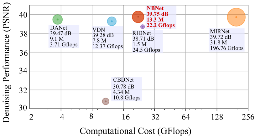
Figure 1: PSNRs at different computational cost and parameter amount of our method and previous methods in SIDD  [1]. The proposed NBNet achieves SOTA performance with a balanced computational requirement.

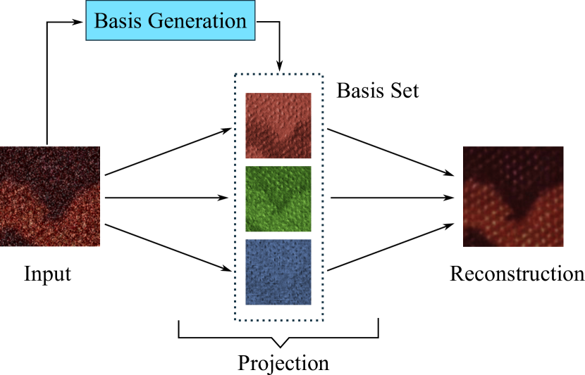
Figure 2: Denoising via subspace projection: Our NBNet learns to generate a set of basis for the signal subspace and by projecting the input into this space, signal can be enhanced after reconstruction for easy separation from noise.

Image denoising is a fundamental and long lasting task in image processing and computer vision. The main challenging is to recover a clean signal $\boldsymbol{x}$ from the noisy observation $\boldsymbol{y}$, with the additive noise $\boldsymbol{n}$, namely:

$$\boldsymbol{y}=\boldsymbol{x}+\boldsymbol{n}$$ (1)

This problem is ill-posed as both the image term $\boldsymbol{x}$ and the noise term $\boldsymbol{n}$ are unknown and can hardly be separated. Towards this end, many denoising methods utilize image prior and a noise model to estimate either image or noise from the noisy observation. For example, traditional methods such as NLM [9] and BM3D [14] use the local similarity of image and the independence of noise, and wavelet denoising [34] utilizes the sparsity of image in transformed domain.

Recent deep neural networks (DNN) based denoising methods [40, 12, 53, 21, 44, 30, 42] usually implicitly utilize image prior and noise distribution learned from a large set of paired training data.

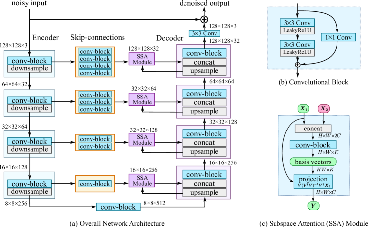
Figure 3: Overall architecture of NBNet and structure of key building blocks. NBNet is based on UNet architecture with a depth of 5 and our SSA module is used to project features of skip-connection from the encoder.

Although previous CNN-based methods have achieved tremendous success, it is still challenging to recover high quality images in hard scenes such as weak textures or high-frequency details. Our key observation is that convolutional networks usually depend on local filter response to separate noise and signal. While in hard scenes with low signal-noise-ratio (SNR), local response can easily get confused without additional global structure information.

In this paper, we utilize non-local image information by projection. The basic concept of image projection is illustrated in Fig. 2, where a set of image basis vectors are generated from the input image, then we reconstruct the image inside the subspace spanned by these basis vectors. As natural images usually lie in a low-rank signal subspace, by properly learning and generating the basis vectors, the reconstructed image can keep most original information and suppress noise which is irrelevant to the generated basis set. Based on this idea, we propose NBNet, depicted in Fig. 3. The overall architecture of NBNet is a commonly-used UNet [36], except for the crucial ingredient subspace attention (SSA) module which learns the subspace basis and image projection in an end-to-end fashion. Our experiments on popular benchmark datasets such as SIDD [1] and DnD [33] demonstrate that the proposed SSA module brings a significant performance boost in both PSNR and SSIM with much smaller computational cost than adding convolutional blocks. As depicted in Fig. 1, the whole architecture of NBNet achieves the state-of-the-art performance while only a smaller additional computational cost is added. To summarize, our contributions include:

• We analyze the image denoising problem from a new perspective of subspace projection. We further design a simple and efficient SSA module to learn subspace projection which can be plugged into normal CNNs.

• We propose NBNet, a UNet with SSA module for projection based image denoising.

• NBNet acheives state-of-the-art performance in PSNR and SSIM on many popular benchmarks

• We provide in-depth analysis of projection based image denoising, demonstrating it is a promising direction to explore.

2 Related Works

19.11 dB	33.63 dB	34.27 dB	34.29 dB	34.70 dB
19.48 dB	32.62 dB	34.14 dB	33.94 dB	34.40 dB
19.49 dB	30.06 dB	32.17 dB	32.00 dB	32.68 dB
Noisy	VDN [47]	DANet [48]	MIRNet [49]	Ours	Reference

Figure 4: Denoising examples from SIDD [1]. Our results superior in weak texture areas like dots and lines pattern

Method	DnCNN	MLP	FoE	BM3D	WNNM	NLM	KSVD	EPLL	CBDNet	RIDNet	VDN	DANet	MIRNet	NBNet
	[50]	[10]	[37]	[13]	[19]	[9]	[2]	[55]	[39]	[4]	[47]	[48]	[49]	ours
PSNR ${\color[rgb]{0,0,0}\uparrow}$	23.66	24.71	25.58	25.65	25.78	26.76	26.88	27.11	30.78	38.71	39.28	39.47	39.72	39.75
SSIM ${\color[rgb]{0,0,0}\uparrow}$	0.583	0.641	0.792	0.685	0.809	0.699	0.842	0.870	0.754	0.914	0.909	0.918	0.959	0.973

Table 1: Denoising comparisons on the SIDD [1] dataset .

		25.65 dB	31.54 dB	32.91 dB
	Noisy	BM3D [14]	FFDNet [52]	DANet [48]
	32.55 dB	31.54 dB	32.09 dB	34.12 dB
Noisy Image	MIRNet [49]	CBDNet [39]	VDN [47]	Ours

Figure 5: Denoising examples from DND [33]. Our results preserve the textures and sharpness.

Method	BM3D	KSVD	MCWNNM	FFDNet+	TWSC	CBDNet	RIDNet	VDN	DANet	MIRNet	NBNet
	[13]	[2]	[46]	[52]	[45]	[39]	[4]	[47]	[48]	[49]	ours
PSNR ${\color[rgb]{0,0,0}\uparrow}$	34.51	36.49	37.38	37.61	37.94	38.06	39.26	39.38	39.59	39.88	39.89
SSIM ${\color[rgb]{0,0,0}\uparrow}$	0.851	0.898	0.929	0.942	0.940	0.942	0.953	0.952	0.955	0.956	0.955

Table 2: Denoising comparisons on the DND [33] dataset.

2.1 Traditional Methods

Image noise reduction is a fundamental component in image processing problem and has been studied for decades. Early works usually rely on image priors, including non-local means (NLM) [9], sparse coding [17, 29, 2], 3D transform-domain filtering (BM3D) [14], and others [19, 34]. Although these classical approaches like BM3D, can generate reasonable desnoising results with certain accuracy and robustness, their algorithmic complexity is usually high and with limited generalization. With the recent development of convolutional neural networks (CNNs), end-to-end trained denoising CNNs has gained considerable attention with great success in this field.

2.2 Network architecture

One main stream of CNNs based desnoising is to design novel network architecture to tackle this problem. Earlier work [10] proposed to apply multi-layer perceptron (MLP) to denoising task and achieved comparable results with BM3D. Since then more advanced network architectures are introduced. Chen et al. [12] proposed a trainable nonlinear reaction diffusion (TNRD) model for Gaussian noise removal at different level. DnCNN [50] demonstrated the effectiveness of residual learning and batch normalization for denoising network using deep CNNs. Later on, More network structures were proposed to either enlarge the receptive field or balance the efficiency, like dilated convolution [51], autoencoder with skip connection [30], ResNet [35], recursively branched deconvolutional network (RBDN) [38]. Recently some interests are put into involving high-level vision semantics like classification and segmentation with image denoising. Works [26, 32] applied segmentation to enhance the denoising performance on different regions. [52] recently proposed FFDNet, a non-blind denoising by concatenating the noise level as a map to the noisy image and demonstrated a spatial-invariant denoising on realistic noises with over-smoothed detail. MIRNet [49] proposed a general network architecture for image enhancement such as denoising and super-resolution with many noval build blocks which can extract, exchange and utilize multi-scale feature information.

In this work, we adapt a UNet style architecture with a novel subspace attention module. Unlike  [4, 5, 41] use attention module for region or feature selection, SSA is designed to learn the subspace basis and image projection.

2.3 Noise distribution

To train the deep networks mentioned above, it requires high quality real datasets with a huge amount of clean and noisy image pairs, which is hard and tedious to construct in practice. Hence, the problem of synthesizing realistic image noise has also been extensively studied. To approximate real noise, multiple types of synthetic noise are explored in previous work, such as Gaussian-Poisson [18, 27], in-camera process simulation [25, 39], Gaussian Mixture Model (GMM) [54] and GAN-generated noises [11] and so on. It has been shown that networks properly trained from the synthetic data can generalize well to real data [53, 8, 43]. Different from all the aforementioned works that focus on noise modeling , our method study subspace basis generation and improve noise reduction by projection.

3 Method

Cases	Datasets	Methods
		CBM3D	WNNM	NCSR	MLP	DnCNN-B	MemNet	FFDNet	$\text{FFDNet}_{v}$	UDNet	VDN	Ours
		[39]	[19]	[16]	[10]	[50]	[40]	[52]	[52]	[24]	[47]
Case 1	Set5	27.76	26.53	26.62	27.26	29.85	30.10	30.16	30.15	28.13	30.39	30.59
	LIVE1	26.58	25.27	24.96	25.71	28.81	28.96	28.99	28.96	27.19	29.22	29.40
	BSD68	26.51	25.13	24.96	25.58	28.73	28.74	28.78	28.77	27.13	29.02	29.16
Case 2	Set5	26.34	24.61	25.76	25.73	29.04	29.55	29.60	29.56	26.01	29.80	29.88
	LIVE1	25.18	23.52	24.08	24.31	28.18	28.56	28.58	28.56	25.25	28.82	29.01
	BSD68	25.28	23.52	24.27	24.30	28.15	28.36	28.43	28.42	25.13	28.67	28.76
Case 3	Set5	27.88	26.07	26.84	26.88	29.13	29.51	29.54	29.49	27.54	29.74	29.89
	LIVE1	26.50	24.67	24.96	25.26	28.17	28.37	28.39	28.38	26.48	28.65	28.82
	BSD68	26.44	24.60	24.95	25.10	28.11	28.20	28.22	28.20	26.44	28.46	28.59

Table 3: The PSNR (dB) results of all competing methods on the three groups of test datasets. The best and second best results are highlighted in bold and Italic, respectively.

3.1 Subspace Projection with Neural Network

As shown in Fig. 2, the projection contains two main steps:

1. Basis generation: generating subspace basis vectors from image feature maps;

2. Projection: transforming feature maps into the signal subspace.

We denote $\boldsymbol{X}_{1},\boldsymbol{X}_{2}\in\mathbb{R}^{H\times W\times C}$ as two feature maps from a single image. They are the intermediate activations of a CNN and can be in different layers but with the same size. We first estimate $K$ basis vectors $[\boldsymbol{v}_{1},\boldsymbol{v}_{2},\cdots,\boldsymbol{v}_{K}]$ based on $\boldsymbol{X}_{1}$ and $\boldsymbol{X}_{2}$, and each $\boldsymbol{v}_{i}\in\mathbb{R}^{N}$ is a basis vector of the signal subspace, where $N=HW$. Then we transform $\boldsymbol{X}_{1}$ into the subspace spanned by $\{\boldsymbol{v}\}$.

3.1.1 Basis Generation

Let $f_{\theta}:(\mathbb{R}^{H\times W\times{C}},\mathbb{R}^{H\times W\times{C}})\rightarrow\mathbb{R}^{N\times K}$ be a function parameterized by $\theta$, basis generation can be written as:

$$\boldsymbol{V}=f_{\theta}(\boldsymbol{X}_{1},\boldsymbol{X}_{2})\text{,}$$ (2)

where $\boldsymbol{X}_{1}$ and $\boldsymbol{X}_{2}$ are image feature maps and $\boldsymbol{V}=[\boldsymbol{v}_{1},\boldsymbol{v}_{2},\cdots,\boldsymbol{v}_{K}]$ is a matrix composed of basis vectors. We implement the function $f_{\theta}$ with a small convolutional network. We first concatenate $\boldsymbol{X}_{1}$ and $\boldsymbol{X}_{2}$ along the channel axis as $\boldsymbol{X}\in\mathbb{R}^{H\times W\times 2C}$, then feed it into a shallow residual-convolutional block with $K$ output channels (Fig. 3(b)), whose output can then be reshaped to $HW\times K$. The weights and biases of the basis generation blocks are updated during the training in an end-to-end fashion.

3.1.2 Projection

Given the aforementioned matrix $\boldsymbol{V}\in\mathbb{R}^{N\times K}$ whose columns are basis vectors of a $K$-dimensional signal subspace $\mathcal{V}\subset\mathbb{R}^{N}$, we can project the image feature map $\boldsymbol{X}_{1}$ onto $\mathcal{V}$ by orthogonal linear projection.

Let $\boldsymbol{P}:\mathbb{R}^{N}\rightarrow\mathcal{V}$ be the orthogonal projection matrix to signal subspace, $\boldsymbol{P}$ can calculated from $\boldsymbol{V}$ [31], given by

$$\boldsymbol{P}=\boldsymbol{V}(\boldsymbol{V}^{\intercal}\boldsymbol{V})^{-1}\boldsymbol{V}^{\intercal},$$ (3)

where the normalization term $(\boldsymbol{V}^{\intercal}\boldsymbol{V})^{-1}$ is required since the basis generation process does not ensure the basis vectors are orthogonal to each other.

Finally, the image feature map $\boldsymbol{X}_{1}$ can be reconstructed in the signal subspace by as $\boldsymbol{Y}$, given by

$$\boldsymbol{Y}=\boldsymbol{P}\boldsymbol{X}_{1}\text{.}$$ (4)

The operations in projection are purely linear matrix manipulations with some proper reshaping, which is fully differentiable and can be easily implemented in modern neural network frameworks.

Combining basis generation and subspace projection, we construct the structure of the proposed SSA module, illustrated in Fig. 3(c).

3.2 NBNet Architecture and Loss Function

The architecture of NBNet is illustrated in Fig. 3(a). The overall structure is based on a typical UNet [36] architecture. NBNet has 4 encoder stages and 4 corresponding decoder stages, where feature maps are downsampled to $\frac{1}{2}\times$ scale with a $4\times 4$-stride-$2$ convolution at the end of each encoder stage, and upsampled to $2\times$ scale with a $2\times 2$ deconvolution before each decoder stage. Skip connections pass large-scale low-level feature maps from each encoder stage to its corresponding decoder stage. The basic convolution building blocks in encoder, decoder and skip connections follow the same residual-convolution structure depicted in Fig. 3(b). We use LeakyReLU as activation functions for each convolutional layer.

The proposed SSA modules are placed in each skip-connection. As feature maps from low levels contain more detailed raw image information, we take the low-level feature maps as $\boldsymbol{X}_{1}$ and high-level features as $\boldsymbol{X}_{2}$ and feed them into an SSA module. In other words, low-level feature maps from skip-connections are projected into the signal subspace guided by the upsampled high-level features. The projected features are then fused with the original high-level feature before outputing to the next decoder stage.

Compared with conventional UNet-like architectures, which directly fuse low-level and high-level feature maps in each decoder stage, the major difference in NBNet is low-level features are projected by SSA modules before fusion.

Finally, the output of the last decoder pass a linear $3\times 3$ convolutional layer as the global residual to the noisy input and outputs the denoising result.

The network is trained with pairs of clean and noisy images, and we use simple $\ell_{1}$ distance between clean images and the denoising result as the loss function, written as:

$$\mathcal{L}(G,\boldsymbol{x},\boldsymbol{y})=\|\boldsymbol{x}-G(\boldsymbol{y})\|_{1}\text{,}$$ (5)

where $\boldsymbol{x}$, $\boldsymbol{y}$ and $G(\cdot)$ represent clean image, noisy image and NBNet, respectively.

4 Evaluation and Experiments

Cases	Datasets	Methods
		CBM3D	WNNM	NCSR	MLP	DnCNN-B	MemNet	FFDNet	$\text{FFDNet}_{v}$	UDNet	VDN	Ours
		[39]	[19]	[16]	[10]	[50]	[40]	[52]	[52]	[24]	[47]
$\sigma=15$	Set5	33.42	32.92	32.57	-	34.04	34.18	34.30	34.31	34.19	34.34	34.64
	LIVE1	32.85	31.70	31.46	-	33.72	33.84	33.96	33.96	33.74	33.94	34.25
	BSD68	32.67	31.27	30.84	-	33.87	33.76	33.85	33.68	33.76	33.90	34.15
$\sigma=25$	Set5	30.92	30.61	30.33	30.55	31.88	31.98	32.10	32.09	31.82	32.24	32.51
	LIVE1	30.05	29.15	29.05	29.16	31.23	31.26	31.37	31.37	31.09	31.50	31.73
	BSD68	29.83	28.62	28.35	28.93	31.22	31.17	31.21	31.20	31.02	31.35	31.54
$\sigma=50$	Set5	28.16	27.58	27.20	27.59	28.95	29.10	29.25	29.25	28.87	29.47	29.70
	LIVE1	26.98	26.07	26.06	26.12	27.95	27.99	28.10	28.10	27.82	28.36	28.55
	BSD68	26.81	25.86	25.75	26.01	27.91	27.91	27.95	27.95	27.76	28.19	28.35

Table 4: The PSNR(dB) results of all competing methods on AWGN noise cases of three test datasets.

We evaluate the performance of our method on synthetic and real datasets and compare it with previous methods. Next, we describe the implementation details. Then we report results on five real image datasets. Finally, we perform ablation studies to verify the superiority of the proposed method.

4.1 Training Settings

The proposed architecture requires no pre-training and it can be trained through an end-to-end strategy. The number of subspace $K$ is set by experience to $16$ for all modules.

In the training stage, the weights of the whole network are initialized according to [20]. We use Adam [23] optimizer with momentum terms ($0.9$, $0.999$). The initial learning rate is set to $2\times 10^{-4}$ and the strategy of decreasing the learning rate is cosine annealing. The training process takes $700,000$ minibatch iterations.

During training, $128\times 128$-sized patches are cropped from each training pair as an instance, and $32$ instances stack a mini-batch. We apply random rotation, cropping and flipping to the images to augment the training data.

4.2 Results on Synthetic Gaussian Noise

We first evaluate our approach on synthetic noisy dataset. We follow the experiment scheme described in VDN [47]. The training dataset includes 432 images from BSD [6], 400 images from the validation set of ImageNet [15] and 4744 images from the Waterloo Exploration Database [28]. The evaluation test dataset are generated from Set5 [22], LIVE1 [22] and BSD68 [7].

In order to achieve a fair comparison, we use the same noise generation algorithm as [47], where non-i.i.d. Gaussian noise is generated by:

$$\boldsymbol{n}=\boldsymbol{n}^{1}\odot\boldsymbol{M},\quad n_{ij}^{1}\sim\mathcal{N}(0,1),$$ (6)

where $\boldsymbol{M}$ is a spatially variant mask. Four types of masks are generated, one for training and three for testing. By this way, the generalization ability of the noise reduction model can be well tested.

Table 3 lists the PSNR performance results of different methods on non-i.i.d Gaussian noise, where our NBNet method outperform the baseline VDN method on every test case, although VDN has an automatic noise level prediction while our method is purely blind noise reduction. More results on additive Gaussian white noise (AWGN) with various noise levels ($\sigma=15,25,50$) also indicates our method surpasses VDN by an average margin of $\sim 0.3$ dB in PSNR.

Our noise reduction method does not explicitly rely on a prior distribution of noise data, but it still achieve the best results in our evaluation. This shows the effectiveness of the proposed projection method which helps separating signal and noise in feature space by utilizing image prior.

4.3 Results on SIDD Benchmark

The Smartphone Image Denoising Dataset (SIDD) [1] , are about 30,000 noisy images from 10 scenes under different lighting conditions using five representative smartphone cameras and generated their ground truth images through a systematic procedure. SIDD can be used to benchmark denoising performance for smartphone cameras. As a benchmark, SIDD splits 1,280 color images for the validation.

In this section, we use SIDD benchmark [1] to verify the performance of our method on a real-world noise reduction task. We compare with the previous methods, including VDN, DANet, and MIRNet. Table 1 illustrates a quantitative comparison between previous methods and ours in Fig 6. We also provide visualization of noise reduction results from different models. The number of parameters and computational cost of each model are shown in Fig 1.

Compared to MIRNet, we provide 39.75 PSNR compared to MIRNet’s 39.72 by only taking 11.2% of its computational cost and 41.82% of its number of parameters. In the SSIM metric, we have a performant rise over MIRNet, boosting from 0.959 to ours 0.969. This growth explains that our model concentrates further on regional textures and local features.

Noisy	FFDNet [52]	VDN [47]	Ours	Reference

Figure 6: Results of Gaussian noise reduction. Our method obtains better visual results in the flower area.

4.4 Results on DND Benchmark

The Darmstadt Noise Dataset (DND) [33] consists of 50 pairs of real noisy images and corresponding ground truth images that were captured with consumer-grade cameras of differing sensor sizes. For every pair, a source image is taken with the base ISO level while the noisy image is taken with higher ISO and appropriately adjusted exposure time. The reference image undergoes careful post-processing involving small camera shift adjustment, linear intensity scaling, and removal of low-frequency bias. The post-processed image serves as ground truth for the DND benchmark.

We evaluate the performance of our method on the DND dataset which contains 50 images for testing. It provides bounding boxes for extracting 20 patches from each image, resulting in 1000 patches in total. Note that the DND dataset does not provide any training data, so we employ a training strategy by combining the dataset of SIDD and Renoir [3]. Results are submitted to the DND benchmark by utilizing the same model that provides the best validation performance on the SIDD benchmark.

Follow to MIRNet, we only use SIDD training set and the same augmentation strategy to train our NBNet. Table 2 shows the results of various methods, we can notice that NBNet can provide a better PSNR compared to MIRNet’s $39.88$ dB with just a fractional of both computational cost and the number of parameters of MIRNet mentioned in section 4.3. Visual results compared to other methods on DND are also provided in Fig 5. Our method can provide a clean output image while preserving the textures and sharpness.

4.5 Ablation Study

Method	# Params	Comp. Cost	PSNR
	($\times 10^{6}$)	(GFlops)	(dB)
UNet	9.5	3.88	39.62
UNet+SSA	9.68	4.28	39.68
UNet+Blocks	13.13	21.8	39.69
UNet+Blocks+SSA	13.31	22.2	39.75

Table 5: Ablation study on SSA and other modules

We examine three major determinants of our model: a) SSA module for another network, and b) the dimension of the signal subspace, i.e. the number of basis vectors $K$. c) the options about projection.

4.5.1 Integrated into DnCNN

For evaluating the effectiveness of our proposed SSA module, we consider another classical architecture DnCNN as a baseline. In order to use $\boldsymbol{X}_{1}$ and $\boldsymbol{X}_{2}$ shown in Equation 2, we regarded the feature of the first convolution as $\boldsymbol{X}_{1}$ and the feature before the last convolution as $\boldsymbol{X}_{2}$. The results are shown in Table 7. DnCNN + Concat achieves about 0.2dB higher than DnCNN by simply concatenating $\boldsymbol{X}_{1}$ and $\boldsymbol{X}_{2}$ to utilizing the different level features, while the DnCNN + SSA with our SSA module achieves about 0.5dB higher than DnCNN.

K	K=1	K=8	K=16	K=32
PSNR	39.28	39.74	39.75	-

Table 6: Effects of subspace dimensionality K on SIDD. Our model does not converge when K=32

4.5.2 Influence about Different k Values

Table 6 provides the results on SIDD with different $K$ values. When the number of basis vectors $K$ is set to 32, our model does not converge. In this setting, as the number of channels in the first stage is also 32, the SSA module does cannot work effectively as subspace projection since $K$ equals to the full dimension size. On the other hand, the higher dimension of the subspace may increase the difficulty of model fitting, hence cause instability of training. The rest experiments shows that the best choice of $K$ is 16. If $K$ equals 1, the information kept in the subspace is insufficient and cause significant information loss in the skip-connection. Setting $K$ to 8 and 16 leads to comparable performance, and the SSA module might create a low-dimensional, compact, or classifiable subspace. Therefore, we can see that the subspace dimension $K$ is a robust hyper-parameter in a reasonable range.

4.5.3 Options about Projection

In Table 8, we evaluate different options about projection: how to generate basis vectors and how to select feature maps for projection. Let’s denote $Proj(a,b)$ as a projection operation where $a$ is projected to the basis generated based on $b$. As shown in first and second rows in Table 8, basis generation based only on $\boldsymbol{X}_{1}$ makes training unstable, resulting in non-convergence. On the contrary, compare third and forth rows, basis generation based on only $\boldsymbol{X}_{2}$ enables the network to be trainable, but get unsatisfactory results. The best results are shown in the last two rows. The network achieves better performance by considering both $\boldsymbol{X}_{1}$ and $\boldsymbol{X}_{2}$. Therefore, projecting $\boldsymbol{X}_{1}$ on the basis generated by $\boldsymbol{X}_{1}$ and $\boldsymbol{X}_{2}$ obtains the best PSNR, which is 39.75 dB.

	Method	PSNR(dB)
1	DnCNN	38.04
2	DnCNN + Concat	38.21
3	DnCNN + SSA	38.59

Table 7: Ablation study on DnCNN architecture

	Method	PSNR(dB)
1	$Proj$($\boldsymbol{X}_{1},\boldsymbol{X}_{1}$)	-
2	$Proj$($\boldsymbol{X}_{1},\boldsymbol{X}_{2}$)	39.02
3	$Proj$($\boldsymbol{X}_{2},\boldsymbol{X}_{2}$)	38.48
4	$Proj$($\boldsymbol{X}_{2},\boldsymbol{X}_{1}$)	-
5	$Proj$($\boldsymbol{X}_{2},\boldsymbol{X}_{1}\&\boldsymbol{X}_{2}$)	39.68
6	$Proj$($\boldsymbol{X}_{1},\boldsymbol{X}_{1}\&\boldsymbol{X}_{2}$)	39.75

Table 8: Ablation study on projections and ’-’ denotes non-convergence

4.6 Basis Visualization and Discussion

To gain insight about how the learned subspace projection works , we pick a sample image and inspect the subspace generated by the SSA module. Fig 7 plots the 16 basis vectors together with the prediction with and without the SSA module. It can be seen that when SSA is enabled, the dotted texture in the dark region is recovered in a way consistent with other part of the patch. This is different when SSA is disabled: the network simply blurs the upper area. Same phenomenon is also observed in Fig 6 where NBNet outperforms other methods in weak-textured regions.

Not surprisingly, this phenomenon finds its root in the projection basis vectors. As shown in the left side of Fig 7, many of the 16 channels contain the dots pattern that evenly span the whole image patch. We can thus reasonably surmise that this improvement should be attributed to the non-local correlation created by the SSA module: the weak textures on the upper part are supported by the similar occurrence in other parts of the image, and the projection reconstructs the texture by combining the basis with globally determined coefficients. A conventional convolutional neural network, on the contrary, rely on responses of fixed-valued local filters and coarse information from downsampled features. When the filter response is insignificant and coarse information is blurry, e.g. in the weak texture areas, non-local information can hardly improve local responses.

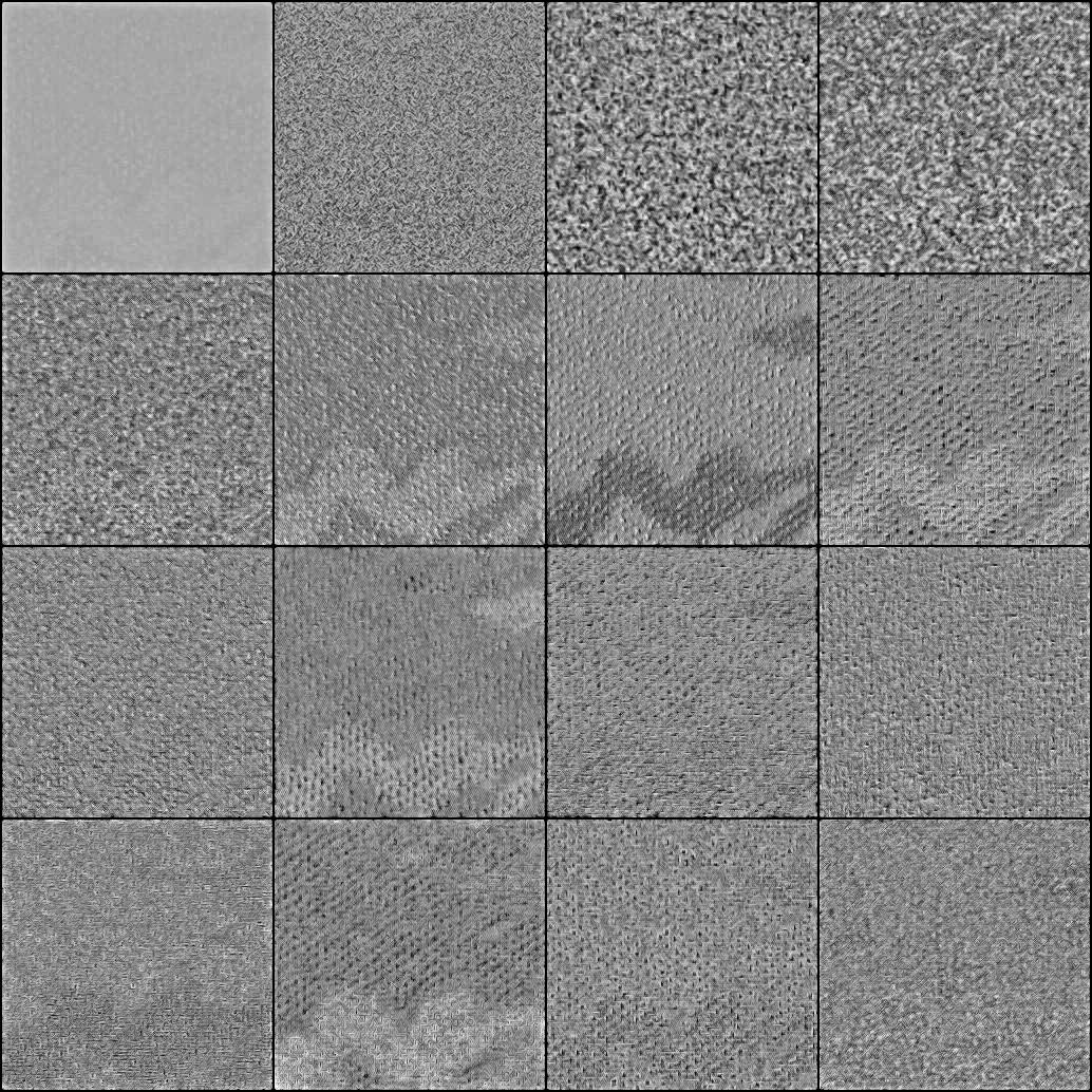
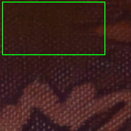
	UNet (31.81 dB)
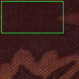
Visualization of basis	SSA (32.15 dB)

Figure 7: Left: the basis vectors that span the projection subspace. It can be seen that the dotted pattern is captured in the channels. Right: denoising results with and without the SSA module. When SSA is used, the weak texture in the upper part is recovered better and appear more consistent with other parts of the image.

5 Conclusion

In this study, we revisit the problem of image denoising and provide a new prospective of subpsace projection. Instead of relying on complicate network architecture or accurate image noise modeling, the proposed subspace basis generation and projection operation can naturally introduce global structure information into denoising process and achieve better local detail preserving. We further demonstrate such basis generation and projection can be learned with SSA in end-to-end fashion and yield better efficiency than adding convolutional blocks. We believe subspace learning is a promising direction for image denoising as well as other low-level vision tasks, and it is worth further exploration.

References

- [1] Abdelrahman Abdelhamed, Stephen Lin, and Michael S Brown. A high-quality denoising dataset for smartphone cameras. In Proc. CVPR, pages 1692–1700, 2018.
- [2] Michal Aharon, Michael Elad, Alfred Bruckstein, et al. K-svd: An algorithm for designing overcomplete dictionaries for sparse representation. IEEE Trans. on Image Processing, 54(11):4311–4322, 2006.
- [3] Josue Anaya and Adrian Barbu. Renoir-a dataset for real low-light image noise reduction. arXiv preprint arXiv:1409.8230, 2014.
- [4] Saeed Anwar and Nick Barnes. Real image denoising with feature attention. In Proc. ICCV, pages 3155–3164, 2019.
- [5] Saeed Anwar, Cong P. Huynh, and Fatih Porikli. Identity enhanced image denoising. In Proc. CVPRW, pages 520–521, 2020.
- [6] Pablo Arbelaez, Michael Maire, Charless Fowlkes, and Jitendra Malik. Contour detection and hierarchical image segmentation. IEEE Trans. on Pattern Analysis and Machine Intelligence, 33(5):898–916, 2010.
- [7] Pablo Arbelaez, Michael Maire, Charless Fowlkes, and Jitendra Malik. Contour detection and hierarchical image segmentation. IEEE Trans. on Pattern Analysis and Machine Intelligence, 33(5):898–916, May 2011.
- [8] Tim Brooks, Ben Mildenhall, Tianfan Xue, Jiawen Chen, Dillon Sharlet, and Jonathan T Barron. Unprocessing images for learned raw denoising. In Proc. CVPR, pages 11036–11045, 2019.
- [9] Antoni Buades, Bartomeu Coll, and J-M Morel. A non-local algorithm for image denoising. In Proc. CVPR, pages 60–65, 2005.
- [10] Harold C Burger, Christian J Schuler, and Stefan Harmeling. Image denoising: Can plain neural networks compete with bm3d? In Proc. CVPR, pages 1256–1272, 2012.
- [11] Jingwen Chen, Jiawei Chen, Hongyang Chao, and Ming Yang. Image blind denoising with generative adversarial network based noise modeling. In Proc. CVPR, pages 3155–3164, 2018.
- [12] Yunjin Chen and Thomas Pock. Trainable nonlinear reaction diffusion: A flexible framework for fast and effective image restoration. IEEE Trans. on Pattern Analysis and Machine Intelligence, 39(6):1256–1272, 2017.
- [13] Kostadin Dabov, Alessandro Foi, Vladimir Katkovnik, and Karen Egiazarian. Image denoising with block-matching and 3d filtering. In Image Processing: Algorithms and Systems, Neural Networks, and Machine Learning, volume 6064, page 606414, 2006.
- [14] Kostadin Dabov, Alessandro Foi, Vladimir Katkovnik, and Karen Egiazarian. Image denoising by sparse 3-d transform-domain collaborative filtering. IEEE Trans. on Image Processing, 16(8):2080–2095, 2007.
- [15] Jia Deng, Olga Russakovsky, Jonathan Krause, Michael S Bernstein, Alex Berg, and Li Fei-Fei. Scalable multi-label annotation. In Proc. SIGCHI, pages 3099–3102, 2014.
- [16] Weisheng Dong, Lei Zhang, Guangming Shi, and Xin Li. Nonlocally centralized sparse representation for image restoration. IEEE Trans. on Image Processing, 22(4):1620–1630, 2013.
- [17] Michael Elad and Michal Aharon. Image denoising via sparse and redundant representations over learned dictionaries. IEEE Trans. on Image Processing, 15(12):3736–3745, 2006.
- [18] Alessandro Foi, Mejdi Trimeche, Vladimir Katkovnik, and Karen Egiazarian. Practical poissonian-gaussian noise modeling and fitting for single-image raw-data. IEEE Trans. on Image Processing, 17(10):1737–1754, 2008.
- [19] Shuhang Gu, Lei Zhang, Wangmeng Zuo, and Xiangchu Feng. Weighted nuclear norm minimization with application to image denoising. In Proc. CVPR, 2014.
- [20] Kaiming He, Xiangyu Zhang, Shaoqing Ren, and Jian Sun. Delving deep into rectifiers: Surpassing human-level performance on imagenet classification. In Proc. ICCV, pages 1026–1034, 2015.
- [21] Viren Jain and Sebastian Seung. Natural image denoising with convolutional networks. In Proc. NeurIPS, pages 769–776, 2009.
- [22] Jiwon Kim, Jung Kwon Lee, and Kyoung Mu Lee. Accurate image super-resolution using very deep convolutional networks. In Proc. CVPR, pages 1646–1654, 2016.
- [23] Diederik P Kingma and Jimmy Ba. Adam: A method for stochastic optimization. arXiv preprint arXiv:1412.6980, 2014.
- [24] Stamatios Lefkimmiatis. Universal denoising networks: a novel cnn architecture for image denoising. In Proc. CVPR, pages 3204–3213, 2018.
- [25] Ce Liu, Richard Szeliski, Sing Bing Kang, C Lawrence Zitnick, and William T Freeman. Automatic estimation and removal of noise from a single image. IEEE Trans. on Pattern Analysis and Machine Intelligence, 30(2):299–314, 2008.
- [26] Ding Liu, Bihan Wen, Xianming Liu, Zhangyang Wang, and Thomas S Huang. When image denoising meets high-level vision tasks: A deep learning approach. arXiv preprint arXiv:1706.04284, 2017.
- [27] Xinhao Liu, Masayuki Tanaka, and Masatoshi Okutomi. Practical signal-dependent noise parameter estimation from a single noisy image. IEEE Trans. on Image Processing, 23(10):4361–4371, 2014.
- [28] Kede Ma, Zhengfang Duanmu, Qingbo Wu, Zhou Wang, Hongwei Yong, Hongliang Li, and Lei Zhang. Waterloo exploration database: New challenges for image quality assessment models. IEEE Trans. on Image Processing, 26(2):1004–1016, 2016.
- [29] Julien Mairal, Francis R Bach, Jean Ponce, Guillermo Sapiro, and Andrew Zisserman. Non-local sparse models for image restoration. In Proc. ICCV, volume 29, pages 54–62, 2009.
- [30] Xiaojiao Mao, Chunhua Shen, and Yu-Bin Yang. Image restoration using very deep convolutional encoder-decoder networks with symmetric skip connections. In Proc. NeurIPS, pages 2810–2818, 2016.
- [31] Carl D. Meyer. Matrix Analysis and Applied Linear Algebra. Society for Industrial and Applied Mathematics. 2000.
- [32] Milad Niknejad, José M Bioucas-Dias, and Mário AT Figueiredo. Class-specific poisson denoising by patch-based importance sampling. arXiv preprint arXiv:1706.02867, 2017.
- [33] Tobias Plötz and Stefan Roth. Benchmarking denoising algorithms with real photographs. In Proc. CVPR, pages 2750–2759, 2017.
- [34] Javier Portilla, Vasily Strela, Martin J Wainwright, and Eero P Simoncelli. Image denoising using scale mixtures of gaussians in the wavelet domain. IEEE Trans. on Image Processing, 12(11):1338–1351, 2003.
- [35] Haoyu Ren, Mostafa El-Khamy, and Jungwon Lee. Dn-resnet: Efficient deep residual network for image denoising. arXiv preprint arXiv:1810.06766, 2018.
- [36] Olaf Ronneberger, Philipp Fischer, and Thomas Brox. U-net: Convolutional networks for biomedical image segmentation. In Proc. MICCAI, pages 234–241, 2015.
- [37] Leonid I Rudin, Stanley Osher, and Emad Fatemi. Nonlinear total variation based noise removal algorithms. Physica D: nonlinear phenomena, 60(1-4):259–268, 1992.
- [38] Venkataraman Santhanam, Vlad I Morariu, and Larry S Davis. Generalized deep image to image regression. In Proc. CVPR, pages 5609–5619, 2017.
- [39] Guo Shi, Yan Zifei, Zhang Kai, Zuo Wangmeng, and Zhang Lei. Toward convolutional blind denoising of real photographs. In arXiv preprint arXiv:1807.04686, 2018.
- [40] Ying Tai, Jian Yang, Xiaoming Liu, and Chunyan Xu. Memnet: A persistent memory network for image restoration. In Proc. ICCV, pages 4539–4547, 2017.
- [41] Chunwei Tian, Yong Xu, Zuoyong Li, Wangmeng Zuo, Lunke Fei, and Hong Liu. Attention-guided cnn for image denoising. Neural Networks, 124:177–129, 2020.
- [42] Dmitry Ulyanov, Andrea Vedaldi, and Victor Lempitsky. Deep image prior. In Proc. CVPR, pages 9446–9454, 2018.
- [43] Abdelrahman Wang, Yuzhi, Haibin Huang, Qin Xu, Jiaming Liu, Yiqun Liu, and Jue Wang. Practical deep raw image denoising on mobile devices. In Proc. ECCV, 2020.
- [44] Junyuan Xie, Linli Xu, and Enhong Chen. Image denoising and inpainting with deep neural networks. In Proc. NeurIPS, pages 341–349, 2012.
- [45] Jun Xu, Lei Zhang, and David Zhang. A trilateral weighted sparse coding scheme for real-world image denoising. arXiv preprint arXiv:1807.04364, 2018.
- [46] Jun Xu, Lei Zhang, David Zhang, and Xiangchu Feng. Multi-channel weighted nuclear norm minimization for real color image denoising. In Proc. ICCV, 2017.
- [47] Zongsheng Yue, Hongwei Yong, Qian Zhao, Deyu Meng, and Lei Zhang. Variational denoising network: Toward blind noise modeling and removal. In Proc. NeurIPS, pages 1690–1701, 2019.
- [48] Zongsheng Yue, Qian Zhao, Lei Zhang, and Deyu Meng. Dual adversarial network: Toward real-world noise removal and noise generation. arXiv preprint arXiv:2007.05946, 2020.
- [49] Syed Waqas Zamir, Aditya Arora, Salman Khan, Munawar Hayat, Fahad Shahbaz Khan, Ming-Hsuan Yang, and Ling Shao. Learning enriched features for real image restoration and enhancement. arXiv preprint arXiv:2003.06792, 2020.
- [50] Kai Zhang, Wangmeng Zuo, Yunjin Chen, Deyu Meng, and Lei Zhang. Beyond a gaussian denoiser: Residual learning of deep cnn for image denoising. IEEE Trans. on Image Processing, 26(7):3142–3155, 2017.
- [51] Kai Zhang, Wangmeng Zuo, Shuhang Gu, and Lei Zhang. Learning deep cnn denoiser prior for image restoration. In Proc. CVPR, pages 3929–3938, 2017.
- [52] Kai Zhang, Wangmeng Zuo, and Lei Zhang. Ffdnet: Toward a fast and flexible solution for cnn-based image denoising. IEEE Trans. on Image Processing, 27(9):4608–4622, 2018.
- [53] Yuqian Zhou, Jianbo Jiao, Haibin Huang, Yang Wang, Jue Wang, Honghui Shi, and Thomas Huang. When awgn-based denoiser meets real noises. arXiv preprint arXiv:1904.03485, 2019.
- [54] Fengyuan Zhu, Guangyong Chen, and Pheng-Ann Heng. From noise modeling to blind image denoising. In Proc. CVPR, pages 420–429, 2016.
- [55] Daniel Zoran and Yair Weiss. From learning models of natural image patches to whole image restoration. In Proc. ICCV, pages 479–486, 2011.