Privacy-Constrained Policies via Mutual Information Regularized Policy Gradients

Abstract

As reinforcement learning techniques are increasingly applied to real-world decision problems, attention has turned to how these algorithms use potentially sensitive information. We consider the task of training a policy that maximizes reward while minimizing disclosure of certain sensitive state variables through the actions. We give examples of how this setting covers real-world problems in privacy for sequential decision-making. We solve this problem in the policy gradients framework by introducing a regularizer based on the mutual information (MI) between the sensitive state and the actions at a given timestep. We develop a model-based stochastic gradient estimator for optimization of privacy-constrained policies. We also discuss an alternative MI regularizer that serves as an upper bound to our main MI regularizer and can be optimized in a model-free setting. We contrast previous work in differentially-private RL to our mutual-information formulation of information disclosure. Experimental results show that our training method results in policies which hide the sensitive state.

1 Introduction

Reinforcement learning (RL) algorithms have shown dramatic successes in areas such as game-playing (Silver et al., 2016), robotics (Haarnoja et al., 2018), and advertising (Gauci et al., 2019). This increasing adoption of RL techniques in real-world settings has illustrated the need for constraints on policies which are hard to express in the typical RL formulation, such as fairness (Nabi et al., 2019), risk-sensitivity (A. & Fu, 2018), and safety under exploration (Dalal et al., 2018). We consider the problem of learning a policy to maximize reward, while minimizing the extent to which the policy’s actions expose information about a sensitive subset of the state variables.

This setting is natural to consider given the increasing prevalence of RL algorithms in society, many taking public actions based in part on sensitive internal information. Examples include a personal assistant algorithm setting appointments while not revealing important personal information, or a workplace scheduling algorithm assigning shifts while avoiding disclosing employees’ medical information. In a business setting we could imagine an algorithm in a competitive market which has to make publicly-visible actions (such as stock purchases, product releases etc) without revealing private information (such as trade secrets or customer information).

A naive approach to this problem is to exclude the sensitive variables from the policy’s input. However, it is well known (Dwork et al., 2006) that this approach will fail when correlations exist between the sensitive and non-sensitive state variables. In the workplace scheduling example above, the policy may give shift assignments based on non-sensitive variables such as availability and performance which are correlated with medical status. Solving our problem requires a careful consideration of the information disclosed by the policy’s actions. Furthermore, the possibility of feedback in the setting introduces additional complications: the agent may be able to take actions which render the sensitive state unimportant for decision making. In the scheduling example, this could involve purchasing assistive equipment (at some cost) which allows employees to work regardless of medical condition. In general a privacy-aware agent may be able to achieve high reward while satisfying information disclosure constraints, compared to an agent that is entirely unaware of the sensitive state.

We formulate this privacy-constrained RL problem as an optimization problem with an additional regularizer on the mutual information $I_{q}(a_{t};u_{t})$ between the action $a_{t}$ and the protected state $u_{t}$ at each timestep $t$, induced under the learned policy $q$. Optimizing this regularizer is not straightforward since it is distribution-dependent (unlike the reward), and involves marginalization over the non-sensitive state. We introduce a model-based gradient estimator for $I_{q}(a_{t};u_{t})$, allowing privacy-dependant policies to be trained in the policy-gradients setting. We also discuss a family of mutual information constraints between either trajectories $\tau_{a},\tau_{u}$ or individual timestep values $a_{t},u_{t}$, both as alternative regularizers and as upper bounds. In particular, we give a model-free gradient estimator for $I_{q}(\tau_{a},\tau_{x};\tau_{u})$, which serves as an upper-bound to $I_{q}(a_{t};u_{t})$. We give experimental results showing that our constrained optimization finds the optimal privacy-constrained policy in an illustrative tabular environment, and hides sensitive state in a continuous control problem and a welfare-allocation problem based on census data.

Previous work has examined the problem of learning differentially-private (DP) policies in the bandit (Sajed & Sheffet, 2019; Shariff & Sheffet, 2018; Agarwal & Singh, 2017) and Markov Decision Process (MDP) setting (Wang & Hegde, 2019; Vietri et al., 2020). However, our mutual-information privacy constraint is qualitatively different from a differential privacy constraint, as we describe in the related work section. We experimentally demonstrate the difference between a DP RL algorithm and our MI-constrained approach, comparing the policies learned on a small environment. Another strand of information-aware RL research has investigated inferring agents’ goals from observation of states and actions (Goyal et al., 2019; Strouse et al., 2018). This strand of research is closest to this work, but has a different problem setting: in our problem an adversary intends to infer the sensitive state only given the actions, and not any of the state variables. We also allow our sensitive state to influence the environmental dynamics, while agents’ goals typically do not.

2 The State-Information Constrained Setting

We analyse privacy-constrained sequential decision-making as a Markov decision process (Sutton & Barto, 2018) (MDP) with information-theoretic constraints. In this paper, we consider episodic MDPs with a fixed length $T$, with a state space $\mathcal{S}=\mathcal{X}\times\mathcal{U}$ consisting of sensitive state variables $u\in\mathcal{U}$ and non-sensitive variables $x\in\mathcal{X}$. In specific problems, the sensitive variables could include gender, location, or a sensitive health status. Our work is agnostic to the specific form of $\mathcal{U}$. In each episode, the initial state is drawn from a distribution $p(x_{1},u_{1})$. At each successive timestep the agent draws an action $a_{t}$ from its policy $q_{\phi}(a_{t}|x_{t},u_{t})$ (a probability distribution over actions given the current state which is parameterized by learnable parameters $\phi$) and the environment samples the successor state $(x_{t+1},u_{t+1})$ conditional on the previous action and state from the dynamics $p$, giving a distribution over trajectories

$$q_{\phi}(\tau)=p(x_{1},u_{1})\prod_{t=1}^{T}q_{\phi}(a_{t}|x_{t},u_{t})p(x_{t+1},u_{t+1}|a_{t},x_{t},u_{t}),$$ (1)

where $\tau=(\tau_{a},\tau_{x},\tau_{u})$ is the collection of the actions and (sensitive and non-sensitive) states sampled in the trajectory. At each timestep $t\geq 1$, we obtain a reward $r(x_{t},u_{t},a_{t})$ concurrently with the transition to the next state. In the standard formulation, we want to learn a policy $q_{\phi}$ which results in a high expected reward. We consider only stationary policies, where the probability of $a_{t}$ is a function of the current state $(x_{t},u_{t})$

As a concrete example, consider an RL algorithm acting as a virtual assistant, sending emails and making appointments at each timestep. The virtual assistant has available a set of variables describing the assistant’s owner, of which some may be designated sensitive (e.g. private relationship status, trade secrets), and some may not be (e.g. current job, education status). The assistant’s goal is to take the best actions, corresponding to the most useful emails and appointments. Furthermore, certain actions may change the state, affecting future decisions. We are interested in learning a policy that maximizes cumulative reward while not allowing an adversary to infer the values of the private state variables. The adversary observes a single action $a_{t}$ and wishes to infer the sensitive variables at that time, $u_{t}$ (not being interested in the sensitive variables in the past or future), while not observing any of the state variables.

We want to develop a worst-case guarantee, so that the adversary cannot infer the value of $u_{t}$ even with full knowledge of the policy parameters $\phi$, the environment dynamics, and unlimited computational power. In this setting, a natural quantity to bound is the mutual information $\mathbb{E}_{u_{t},a_{t}\sim q_{\phi}}\left[\log q_{\phi}(u_{t}|a_{t})-\log q_{\phi}(u_{t})\right]=I_{q_{\phi}}(a_{t};u_{t})$, i.e. the amount of information an optimal adversary gains about $u_{t}$ from observing $a_{t}$ (Liao et al., 2017). By the data processing inequality, no adversary can gain more information about $u_{t}$ from observing $a_{t}$ than $I_{q_{\phi}}(a_{t};u_{t})$, and so it serves as an upper bound on the information inferable by computation- or data-limited adversaries. As a special case, if $q_{\phi}(u_{t}|a_{t})=q_{\phi}(u_{t})$, i.e. $u_{t}$ is independent of $a_{t}$, then the mutual information is zero.

Therefore we formulate the problem of learning a state-private policy as a constrained optimization problem (Altman, 1999), aiming to solve the problem

$$\underset{\phi}{\text{Maximize}}\ \underset{\tau\sim q_{\phi}}{\mathbb{E}}\left[\sum_{t=1}^{T}r(x_{t},u,a_{t})\right],\quad\text{s.t.}\ I(a_{t};u_{t})<\epsilon_{t}\ \forall T,$$ (2)

with $\epsilon_{t}$ a set of parameters that we can adjust to trade off good performance against low privacy. In practice, we will use the policy gradient method to carry out this optimization, imposing $I_{q_{\phi}}(a_{t};u_{t})$ as a regularizer on the objective. As mentioned before, note that it is not sufficient to simply exclude the sensitive state by only allowing the policy to be a function of $x_{t}$, as $x_{t}$ may be highly correlated with $u_{t}$, such as the $(x_{t},u_{t})$ pair of (zip code, race).

Notably, our regularization term $I_{q_{\phi}}(a_{t};u_{t})$ does not involve the non-sensitive state $x_{t}$. In other words, we consider the mutual information between the actions and sensitive state, marginalized over the distribution of non-sensitive state induced by $q_{\phi}$. Furthermore the mutual information term is with respect to the distribution over trajectories induced by the policy $q_{\phi}$, i.e. $I_{q_{\phi}}(a_{t};u_{t})=D_{\text{KL}}\left(q_{\phi}(a_{t},u_{t})\|q_{\phi}(a_{t})q_{\phi}(u_{t})\right)$, with $q_{\phi}(a_{t},u_{t})=\int_{\tau_{x_{1:t}},\tau_{(a,u)_{1:t-1}}}q_{\phi}(a_{t}|u_{t},x_{t})q_{\phi}(u_{t},x_{t}|\tau_{(a,u)_{1:t-1}},\tau_{x_{1:t-1}})$. This means that when choosing the action at time $t$, the agent must consider the effects on the distribution at future timesteps, such as taking a corrective action that allows future actions to be chosen independently of $u_{t}$.

2.1 Alternative Threat Models

In the previous section we discussed the threat model where the adversary aims to infer the sensitive state at time $t$, $u_{t}$, by observing the corresponding action $a_{t}$. This corresponds to the case where the policy has a one-off interaction with an adversary where the adversary does not aim to infer the previous or future states $u_{t^{\prime}}$ for $t^{\prime}\neq t$. We can also consider adversaries that observe the whole trajectory of actions $\tau_{a}$ and wish to infer a particular $u_{t}$, or wish to infer the whole trajectory of sensitive states $\tau_{u}$. Finally we can imagine adversaries that observe all of the non-sensitive states in addition to the actions, and wish to infer all the sensitive states. Since incorporating additional variables always increases mutual information, we have

$$I_{q_{\phi}}(a_{t};u_{t})\leq I_{q_{\phi}}(\tau_{a};u_{t})\leq I_{q_{\phi}}(\tau_{a};\tau_{u})\leq I_{q_{\phi}}(\tau_{a},\tau_{x};\tau_{u}).$$ (3)

Therefore, we can interpret e.g. $I_{q_{\phi}}(\tau_{a},\tau_{x};\tau_{u})$ both as the relevant quantity to constrain if the adversary has access to all actions and non-sensitive states and wishes to infer all sensitive states, and as an upper bound to any of the other mutual information quantities for other threat models. In section 4.3 we give a gradient estimator for $I_{q_{\phi}}(\tau_{a},\tau_{x};\tau_{u})$. In the appendix (section A.2) we also sketch out a gradient estimator for $I_{q_{\phi}}(\tau_{a};\tau_{u})$, although we do not investigate it further in this work.

2.2 Dual Formulation

We can approach the constrained optimization problem (2) by considering the Lagrangian dual problem

$$\underset{\boldsymbol{\lambda}\geq 0}{\min}\ \underset{\phi}{\max}\ \mathbb{E}_{\tau\sim q_{\phi}}\left[R(\tau)\right]-\sum_{t=1}^{T}\lambda_{t}(I_{q_{\phi}}(a_{t};u_{t})-\epsilon_{t}),$$ (4)

where $\boldsymbol{\lambda}$ is a vector of Lagrange multipliers.

In order to solve the inner maximization problem with gradient descent, we require estimators for $\nabla_{\phi}\mathbb{E}_{\tau\sim{q_{\phi}}}\left[R(\tau)\right]$ and $\nabla_{\phi}I_{q_{\phi}}(a_{t};u_{t})$. Since even evaluating the mutual information in high dimensions is challenging (Paninski, 2003), this is not trivial. Our main contribution is a method to approximate the objective $I_{q_{\phi}}(a_{t};u_{t})$, and a method for estimating $\nabla_{\phi}I_{q_{\phi}}(a_{t};u_{t})$ where a dynamics model is available. We also give a model-free gradient estimator for $I_{q_{\phi}}(\tau_{a},\tau_{x};\tau_{u})$, which we can use as an upper bound to $I_{q_{\phi}}(a_{t};u_{t})$ or as the relevant constraint in an alternative threat model as described above.

3 Related Work

3.1 Privacy In Reinforcement Learning

Concerns around privacy in statistical analysis have existed for decades (Anderson, 1988). The specific problem of satisfying privacy concerns while maximizing reward in a reinforcement learning context was introduced in Sakuma et al. (2008) and Zhang & Makedon (2005). Since then, several works have tackled the privacy-preserving RL problem in various special cases, such as linear contextual bandits (Neel & Roth, 2018; Shariff & Sheffet, 2018), multi-armed bandits (Sajed & Sheffet, 2019; Mishra & Thakurta, 2015; Tossou & Dimitrakakis, 2016), and online learning with bandit feedback (Agarwal & Singh, 2017; Smith & Thakurta, 2013). In non-bandit settings where the agent’s actions result in changes to the state (i.e. the ‘general RL’ setting) there is much less prior work. In the tabular setting Vietri et al. (2020) formulate a method with guarantees on regret and privacy which match the known lower bounds in terms of dependence on certain environment-specific parameters such as action space size. The only prior work we are aware of in the continuous state setting is Wang & Hegde (2019), developing a variant of Q-learning which can find policies which obey differential privacy constraints on the reward function.

These works all use the differential privacy (DP) privacy metric, with two variations coming closest to our setting. As summarized in Basu et al. (2019), a bandit algorithm is (globally) $\epsilon$-DP if $\log q_{\phi}(\tau_{a}|\tau_{x})-\log q_{\phi}(\tau_{a}|\tau_{x}^{\prime})\leq\epsilon$ for all $\tau_{a}$ and $\tau_{x},\tau_{x}^{\prime}$ where $\tau_{x}^{\prime}$ is a trajectory that differs from $\tau_{x}$ at only one timestep. An algorithm is locally $\epsilon$-DP if this holds for a single timestep, i.e. $\log q_{\phi}(a_{t}|\tau_{x_{1:t-1}},\tau_{a_{1:t-1}})-\log q_{\phi}(a_{t}|\tau_{x_{1:t-1}}^{\prime},\tau_{a_{1:t-1}})$, for all $\tau_{a}$ and $\tau_{x_{1:t-1}},\tau_{x_{1:t-1}}^{\prime}$ where $\tau_{x_{1:t-1}}^{\prime}$ is a trajectory that differs from $\tau_{x_{1:t-1}}$ at only one timestep.

In general the relationship between DP and mutual information privacy constraints is not straightforward, although characterisations have been made in several settings (Wang et al., 2016; Mir, 2012; du Pin Calmon & Fawaz, 2012). To our knowledge, a standard definition of DP privacy in the general RL setting is not agreed upon. Comparing to the DP constraint in the bandit setting, a key difference is that our constraint penalizes predictability of $u_{t}$ given $a_{t}$, in expectation over the distribution of $u_{t},a_{t}$, while a DP constraint penalizes predictability between neighbouring trajectories, with no notion of the relative likelihood of these trajectories. This is a particularly important difference in the general RL setting, where the ability of a policy to change the distribution of states is a key feature.

In the Q-learning setting of (Wang & Hegde, 2019), the DP constraint is applied on the Q-learning algorithm itself, viewed as a function $\mathcal{A}:\mathcal{R}\to\mathcal{Q}$ from the space of reward functions to the space of Q-functions. The requirement is then that for any reward functions $r,r^{\prime}$ with $\|r-r^{\prime}\|_{\infty}<1$, $\log p(\mathcal{A}(r))-\log p(\mathcal{A}(r^{\prime}))<\epsilon$, with a probability measure over $\mathcal{Q}$ provided by an RHKS. We qualitatively compare policies learned under this constraint to policies satisfying our MI constraint in section 5.

Finally, we describe the recent differential privacy constraint for general RL formulated in Vietri et al. (2020). There, $T$ episodes of length $H$ are experienced by the RL agent, each with arbitrarily different dynamics (including rewards). The constraint is that $\log q_{\phi}(\tau_{a\setminus t})-\log{\tilde{q}}_{\phi}(\tau_{a\setminus t})\leq\epsilon$, for all $\tau_{a\setminus t}$ (denoting the set of $H(T-1)$ actions not including the actions in the $t$th episode) and all $q,{\tilde{q}}$ (denoting the probability under an MDP $q$ and an MDP ${\tilde{q}}$ with dynamics (and rewards) that differ from $q$ only in the $t$th episode). This constraint is significantly more adversarial than ours, as we assume a fixed MDP.

3.2 Mutual Information Constraints in RL

The previous work that is most closely related to our setting is in the field of mutual information constraints for reinforcement learning. The original motivation for information-regularization was in the context of goal-directed RL. Here, the agent has a goal $g_{t}$ which effects the agent’s choice of action, but not the dynamics. First, van Dijk & Polani (2011) explored this in the options framework, regularizing $I(a_{t};g_{t}|\tau_{a_{1:t-1}},\tau_{x_{1:t-1}})$. More recently, both Goyal et al. (2019) and Strouse et al. (2018) studied the behaviour of policies regularized with the term $I(a_{t};g_{t}|s_{t})$. Both explore a rearrangement of this regularizer as the KL-divergence between the learned policy and a ‘default’ policy. In the case of Goyal et al. (2019) this is used to learn policies which have diverse goals, in a similar fashion to the classic information bottleneck learning framework. In the case of Strouse et al. (2018) the motivation is explicitly to learn agents that either share or hide action-goal information (depending on the sign of the regularizer’s coefficient). Although a similar motivation, the threat model considered is different to ours–in theirs, the adversary knows the state at time $t$ and wants to infer the goal from the actions, while in ours the whole state is unobserved and the adversary wants to infer some subset of the state from the actions. Perhaps closest to our work is their section assuming that actions are unobserved–controlling $I(s_{t};g_{t})$. We can see our approach as the corresponding problem for unobserved states–controlling $I(a_{t};g_{t})$, with the additional aspect that our ‘goal’ may in general influence the dynamics of the environment.

3.3 Demographic Parity

Another related body of work is that of demographic parity in fair machine learning. The demographic parity objective (Zemel et al., 2013) for binary prediction requires that the class predicted, $\hat{y}$, is statistically independent of protected variables such as race or gender. Previous work (Song et al., 2019) has formulated this as requiring $I(\hat{y};u)=0$ for protected variables $u$, while marginalizing over the unprotected variables $x$. We show in the appendix (section A.9) that our approach is equivalent to the demographic parity objective for one-timestep episodes. Therefore, our mutual-information constraint can be seen as an extension of demographic parity to the general RL setting. It is unclear whether this extension from the bandit setting makes sense as a notion of fairness: recent work has proposed different formulations of fairness for sequential decision-making, such as meritocratic fairness (Jabbari et al., 2017) or path-specific fairness (Nabi et al., 2019).

4 Estimation and Optimization of Privacy Constraints

Despite the common use of mutual information in machine learning and statistics, it is in general intractable to compute the MI between two random variables (Paninski, 2003). The reinforcement learning setting provides us with an additional challenge, as to perform efficient gradient-based optimization we must form explicit Monte-Carlo estimators of the gradient in terms of distributions that we are able to sample from. Two common tricks in working with mutual information are to approximate posterior distributions with adversarial training (Nowozin et al., 2016), and to form upper bounds by introducing auxiliary variables. We use both tricks to obtain two different gradient estimators for our objective.

4.1 Estimation of the MI constraint

Our mutual information constraint is $I_{q_{\phi}}(a_{t};u_{t})\leq\epsilon_{t}$, for all $1\leq t\leq T$. From the definition of mutual information, we have $I_{q_{\phi}}(a_{t};u_{t})=D_{\text{KL}}(q_{\phi}(a_{t},u_{t})\|q_{\phi}(a_{t})q_{\phi}(u_{t}))=\mathbb{E}_{a_{t},u_{t}\sim q_{\phi}}\left[\log q_{\phi}(u_{t}|a_{t})-\log q_{\phi}(u_{t})\right]$. In general, there is no way to obtain these probabilities in closed-form in terms of $\phi$, since we only know $q_{\phi}(a_{t}|x_{t},u_{t})$. However, we can replace $q_{\phi}(u_{t}|a_{t})$ and $q_{\phi}(u_{t})$ with approximating distributions $p_{\psi}(u_{t}|a_{t})$ and $p_{\psi}(u_{t})$. We learn the parameters $\psi$ of $p_{\psi}$ by maximum likelihood on samples from $q_{\phi}(\tau)$. Given a sufficiently powerful model $p_{\psi}$ and enough samples, $p_{\psi}(u_{t}|a_{t})\approx q_{\phi}(u_{t}|a_{t})$ and $p_{\psi}(u_{t})\approx q_{\phi}(u_{t})$, so

$$I_{q_{\phi}}(a_{t};u_{t})\approx\mathbb{E}_{a_{t},u_{t}\sim q_{\phi}}\left[\log p_{\psi}(u_{t}|a_{t})-\log p_{\psi}(u_{t})\right].$$ (5)

If $p_{\psi}$ recovers $q_{\phi}$ exactly we achieve the equality. By training a discriminator $p_{\psi}$ we can use this expression to check if a policy is fulfilling the mutual information constraint in equation (2).

4.2 Model Based Estimation of the MI Constraint Gradient

In order to perform gradient-based constrained optimization to solve the problem in equation (2) we need a gradient estimator in terms of densities we can sample from. If our policy is parameterized with $\phi$, we see that applying the policy gradient theorem to the quantity $\mathbb{E}_{a_{t},u_{t}\sim q_{\phi}}\left[\log p_{\psi}(u_{t}|a_{t})-\log p_{\psi}(u_{t})\right]$ gives us a gradient estimator $\mathbb{E}_{a_{t},u_{t}\sim q_{\phi}}\left[\left(\log p_{\psi}(u_{t}|a_{t})-\log p_{\psi}(u_{t})\right)\nabla_{\phi}\log q_{\phi}(a_{t},u_{t})\right]$. However, $\nabla_{\phi}\log q_{\phi}(a_{t},u_{t})$ is difficult to compute, as $q_{\phi}(a_{t},u_{t})$ involves a marginalization over all previous states and actions in the trajectory. In the appendix (section A.1) we show that

$$\nabla_{\phi}\underset{{a_{t},u_{t}\sim q_{\phi}}}{\mathbb{E}}\left[\log p_{\psi}(u_{t}|a_{t})-\log p_{\psi}(u_{t})\right]$$ (6)

$$= \underset{a_{t},u_{t}\sim q_{\phi}}{\mathbb{E}}\left[R_{\psi}(u_{t},a_{t})\underset{x_{t}\sim q_{\phi}(\cdot|u_{t},a_{t})}{\mathbb{E}}\left[\nabla_{\phi}\log q_{\phi}(a_{t}|x_{t},u_{t})\right.\right.$$

$$+\underset{\tau_{(x,u,a)_{1:t-1}}\sim q_{\phi}(\cdot,\cdot|x_{t},u_{t})}{\mathbb{E}}\left[\sum_{t^{\prime}=1}^{t^{\prime}=t-1}\frac{p(x_{t^{\prime}+1},u_{t^{\prime}+1}|a_{t^{\prime}},x_{t^{\prime}},u_{t^{\prime}})}{q_{\phi}(x_{t^{\prime}+1},u_{t^{\prime}+1}|x_{t^{\prime}},u_{t^{\prime}})}\right.$$

$$\hskip 119.50148pt\times\nabla_{\phi}\log q_{\phi}(a_{t^{\prime}}|x_{t^{\prime}},u_{t^{\prime}})\Bigg{]}\Bigg{]}\Bigg{]},$$

where $R_{\psi}(u_{t},a_{t})=\log p_{\psi}(u_{t}|a_{t})-\log p_{\psi}(u_{t})$. To compute this estimate we need to know the transition dynamics of the MDP, $p(x_{t},u_{t}|a_{t-1},x_{t-1},u_{t-1})$. Although the model-based requirement may seem stringent, it is plausible that a model will be available in higher-stakes settings where privacy is a consideration. Furthermore, model-based techniques are increasingly popular due to empirical (Kaiser et al., 2019) and theoretical (Du et al., 2019) sample-efficiency improvements over model-free techniques. With the increasing prevalence of model-based techniques in addition to sim2real (Higgins et al., 2017)-based training pipelines, it is not unreasonable to assume the presence of some sort of dynamics model if required. Note that since we can compute $q_{\phi}(x_{t},u_{t}|x_{t-1},u_{t-1})$ as $\int_{a_{t-1}}p(x_{t},u_{t}|a_{t-1},x_{t-1},u_{t-1})q_{\phi}(a_{t-1}|x_{t-1},u_{t-1})da_{t-1}$, we do not need to learn a separate $q_{\phi}(x_{t},u_{t}|x_{t-1},u_{t-1})$ distribution.

4.3 Action-trajectory mutual information constraint

In the previous section we formed a model-based approach to finding the gradient of our privacy constraint. We can avoid this marginalization by explicitly including the trajectory of actions and states in our mutual information term, and so considering the constraint $I_{q_{\phi}}(\tau_{x},\tau_{a};\tau_{u})\leq\epsilon$. As discussed in section 2.1, this constraint is an upper bound for the constraint in equation (2), and is the relevant constraint for alternative adversarial threat models.

By definition, $I_{q_{\phi}}(\tau_{x},\tau_{a};\tau_{u})=\mathbb{E}_{\tau\sim q_{\phi}}\left[\log q_{\phi}(\tau_{u}|\tau_{x},\tau_{a})-\log q_{\phi}(\tau_{u})\right]$. Similarly to above, we can approximate the $q_{\phi}(\tau_{u}|\tau_{x},\tau_{a})$ and $q_{\phi}(\tau_{u})$ terms with learned discriminators $p_{\psi}(\tau_{u}|\tau_{x},\tau_{a})$ and $p_{\psi}(\tau_{u})$, which are trained to predict $\tau_{u}$. In the limit where $p_{\psi}(\tau_{u}|\tau_{a},\tau_{x})\approx q_{\phi}(\tau_{u}|\tau_{x},\tau_{a})$ and $p_{\psi}(\tau_{u})\approx q_{\phi}(\tau_{u})$ we get a close estimate of the original. Therefore, $I_{q_{\phi}}(\tau_{a},\tau_{x};\tau_{u})\approx\mathbb{E}_{\tau\sim q_{\phi}}\left[\log p_{\psi}(\tau_{u}|\tau_{x},\tau_{a})-\log p_{\psi}(\tau_{u})\right]$, for a sufficiently accurate adversarial model $p_{\psi}$. This has a tractable gradient,

$$\nabla_{\phi}\underset{\tau\sim q_{\phi}}{\mathbb{E}}\left[\log\frac{p_{\psi}(\tau_{u}|\tau_{x},\tau_{a})}{p_{\psi}(\tau_{u})}\right]= \underset{\tau\sim q_{\phi}}{\mathbb{E}}\left[\log\frac{p_{\psi}(\tau_{u}|\tau_{x},\tau_{a})}{p_{\psi}(\tau_{u})}\right.$$ (7)

$$\hskip 39.83368pt\times\nabla_{\phi}\log q_{\phi}(\tau)\bigg{]},$$

which we can use to learn policies solving the constrained optimization problem in equation (2).

We can optimize this quantity without any knowledge of the dynamics. If we aim to use this as an upper bound, the tradeoff is that the upper bound may be loose. In the appendix (section A.8) we examine the looseness of the bound in the setting where $u_{t}$ influences the transitions and rewards only through the initial state.

Algorithm 1 Model-Based MI-Constrained Policy Gradients (Detailed pseudocode in section A.6)

  Initialize Lagrange multipliers $\boldsymbol{\lambda}\in\mathbb{R}_{\geq 0}^{T}$, policy, discriminator and baseline parameters $\phi,\psi,\theta$

  while min over $\boldsymbol{\lambda}$ not converged do

     Change $\boldsymbol{\lambda}$ by coordinate descent

     while inner max-min over $\psi,\phi$ not converged do

        Draw batch $\tau_{1:B}\sim q_{\phi}(\tau)$

        Take gradient step in $\psi$ with respect to likelihood $\sum_{j=1}^{B}\sum_{t=1}^{T}\log q_{\psi}(u_{t,j}|a_{t,j},t)$

        Compute regularizer gradient $g_{I}$ via equation (7)

        Compute policy gradient $g_{p}$, with baseline $\theta$

        Take gradient step in $\phi$ with gradient $g_{p}+\boldsymbol{\lambda}^{T}g_{I}$

        Take gradient step in $\theta$ with respect to mean squared error on returns

     end while

  end while

Algorithm 2 Model-Free MI-Constrained Policy Gradients (Detailed pseudocode in section A.6)

  Initialize Lagrange multiplier $\lambda\in\mathbb{R}_{\geq 0}$, initial policy, discriminator and critic parameters $\phi,\psi,\theta$

  while min over $\lambda$ not converged do

     Change $\lambda$ by coordinate descent

     while inner max-min over $\psi,\phi$ not converged do

        Draw batch of $B$ trajectories $\tau_{1:B}\sim q_{\phi}(\tau)$

        Take gradient step in $\psi$ with respect to likelihood $\sum_{j=1}^{B}\log q_{\psi}(\tau_{u,j}|\tau_{a,j},\tau_{x,j})$

        Compute policy gradient $g_{p}$, with baseline $\theta$

        Compute regularizer gradient $g_{I}$ via section 4.3.

        Take gradient step in $\phi$ with gradient $g_{p}+\lambda g_{I}$

        Take gradient step in $\theta$ with respect to mean squared error on returns

     end while

  end while

5 Experiments

In this section we use our constrained optimization procedure to solve privacy-constrained tasks in several different environments. We first consider a toy tabular task to illustrate that we can learn policies that intelligently plan ahead, changing the distribution over future states in order to reduce the information leaked in subsequent timesteps. Going beyond tabular environments, we evaluate our algorithm on a continuous control task. Finally, we compare the behaviour of a differentially-private Q-learning policy to our mutual information-constrained policy. In the appendix, we compare the behaviour of the $I(\tau_{u};\tau_{x},\tau_{a};)$ constraint to the $I(u_{t};a_{t})$ constraint on a toy example, investigate a welfare-allocation task to see applications to real-world data, and present a one-dimensional environment illustrating that we can control information disclosure at specific timesteps, controlling $I(u_{t};a_{t})$ by varying the elements $\lambda_{t}$ of the vector of Lagrange multipliers.

5.1 Privacy in Internet Connections

We consider a toy example to illustrate the behavior of the policies learned with our regularizer. As a first goal, we want to show that our estimator is able to indeed reduce the mutual information between actions and sensitive state. We also want to illustrate that the learned policies exploit the structure of the problem in order to achieve the privacy constraints, such as taking early corrective actions which remove future $u$-dependence from actions. In other words, we want to show that the learned policy is not just choosing actions at random (which would trivially satisfy the mutual information constraint). To show this, we construct a tabular example with a policy representing the actions of a virtual assistant tasked with connecting its owner to various web sites.

The agent’s owner has one of $n$ IP addresses. At each of $T$ timesteps, the agent has a choice of connecting to the websites via $n$ mirrors. The mirror corresponding to the owner’s IP address will connect quickest, resulting in highest reward $r^{*}$. Connecting via the other mirrors results in a slower or intermittent connection, with lower reward $r^{-}\ll r^{*}$. The agent can also purchase a VPN, which gives no immediate reward but allows reasonably good connection to all mirrors at future timesteps, with reward $r^{-}\ll r^{\text{VPN}}<r^{*}$ for connecting to any mirror. The binary non-sensitive state $x\in\{0,1\}$ represents whether the VPN has been purchased or not.

In this simple example, by inspection we see that the unconstrained optimal policy is simply to always choose the mirror corresponding to the owner’s IP address, resulting in a total reward of $Tr^{*}$. The optimal policy under a privacy constraint on the IP address is to choose to activate the VPN on the first timestep, then choose any of the mirrors under the subsequent timesteps, resulting in a total reward of $(T-1)r^{\text{VPN}}$. In our experiments we used $n=4$. We consider solving the optimization problem in equation (4) with $\epsilon_{t}=0$ (corresponding to the non-privacy constrained case) and $\epsilon_{t}=1$ (corresponding to the privacy-constrained case). In this simple setting, we use empirical frequencies of $u_{t},a_{t}$ over a minibatch to compute the joint probability distribution $p(u_{t},a_{t})$. For the dynamics model, we use the ground-truth dynamics.

Our policy model is a fully-connected neural network with two 256-unit hidden layers. To reduce variance, we subtract off a value-function baseline, estimated with an MLP with two 64-hidden-unit layers. To encourage initial exploration, we add the entropy of the action distribution to the reward and anneal this term over time. We used the JAX differentiable programming framework (Bradbury et al., 2020) for all experiments. Details of additional hyperparameters can be found in the appendix, in section A.7.

Results: The policy that we learn under the privacy constraint exactly recovers the globally optimal privacy-constrained policy described in the section above. This policy activates the VPN on the first timestep and then always connects to the same mirror, regardless of $u_{t}$, so that the actions are independent of $u_{t}$. The non-privacy constrained policy always chooses the mirror which corresponds to the user’s IP address, resulting in a $(u_{t},a_{t})$-distribution where $u_{t}$ is completely disclosed by $a_{t}$. The average value of $I(a_{t};u_{t})$ across the episode is 1.38 for the non-constrained policy and 0.0047 for the constrained policy. In the unconstrained policy this corresponds to $\log 1/4\approx 1.39$. Trajectory samples are shown in figure 2. This illustrates that the learned constrained policies do indeed reduce $I(a_{t};u_{t})$, taking pre-emptive actions in order to limit the reduction in reward caused by obeying the constraint.

5.2 Private Control in a Continuous Domain

Our second experiment is on an abstract two-dimensional continuous control domain, illustrating the use of a learned discriminator $p_{\psi}(u_{t}|a_{t})$, and an environment where $u_{t}$ changes over the episode. The agent controls a particle under Newtonian dynamics. The agent has four possible actions, imposing a unit force in one of the four cardinal directions, with a reward proportional to the negative squared distance from the origin. The state is four dimensional, consisting of the coordinate positions $x$ and $u$ and corresponding velocities, $(x,\dot{x},u,\dot{u})$. We consider the state variable $u$ to be sensitive. At each timestep a random force is applied to the particle, distributed as an isotropic Gaussian. The goal is to keep the particle close to the origin subject to this random perturbing force.

For this experiment we instantiate an explicit adversarial model to predict $u_{t}$ given $a_{t}$. We use an MLP with two 256-unit hidden layers parameterizing the mean and variance of a Gaussian given the action at timestep $T$. We update the parameters of the adversary on each iteration. The unconditional prediction $p(u_{t})$ is found by fitting a Gaussian at each timestep to the empirical moments of the sampled minibatch’s trajectories. The policy and critic architecture is the same as the previous experiment. Additional hyperparameters are described in the appendix, section A.5.

Results:

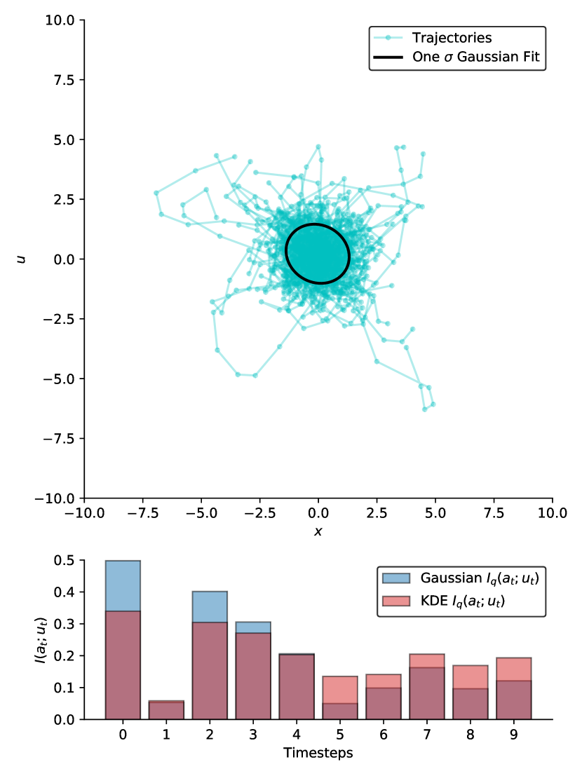
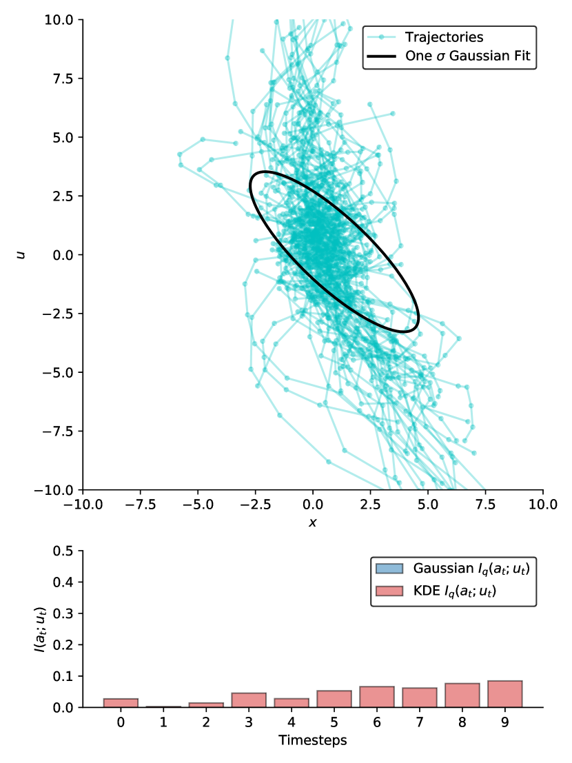
Figure 1: A batch of 128 trajectories for the 2d control task, $u$-unconstrained (left) and -constrained (right). We see that the constraint forces the policy to induce much more variance in the $u$-direction in the constrained case, with correspondingly much less mutual information between $a_{t}$ and $u_{t}$. Since the trajectories on the right are on average further away from the center, satisfying the privacy constraint results in a policy with lower reward. This environment has an unavoidable tradeoff between reward and privacy. Our policy reduces the MI to zero when computed via a Gaussian discriminator, but this diverges from the MI as estimated by a nonparametric KDE at later timesteps as the distribution of $u$ is less Gaussian.

The results are shown in figure 1. Trajectories from the $u$-constrained policy have a much higher variance in the $u$-direction, with correspondingly lower mutual information. Trajectories from the policy without the $u$-constraint have approximately equal variance in both directions. This illustrates that the use of a learned $p_{\psi}(u_{t}|a_{t})$ discriminator is practical on this domain. We also observe that the privacy-constrained trajectories are on average further away from the center, and so receive less reward. In other words, the policy trades off reward in order to satisfy the privacy constraint. We also plot $I(a_{t};u_{t})$, first assuming a Gaussian distribution (as is used for the discriminator in training), and then using a nonparametric kernel density estimator, which doesn’t assume Gaussianity. We see that our policy learns to reduce the mutual information under a Gaussian assumption to zero, but the true MI as measured by the KDE starts to increase at later timesteps, as the distribution of $u$ becomes more non-Gaussian. A more flexible density model for $p(u_{t}|a_{t})$, such as a normalizing flow (Papamakarios et al., 2019), could be used to avoid a Gaussian assumption in the density model.

5.3 Qualitative Comparison to Differentially Private Policies

We qualitatively compare the policies learned with our mutual information constraint to an $(\epsilon,\delta)-$differentially private Q-learning policy obtained via the DPQL algorithm described in Wang & Hegde (2019)using their implementation. The provided implementation only supports a one-dimensional continuous state, so we consider a reparameterization of the VPN environment described in section 5.1 with $n=4$ mirrors, mapping the eight possible states ($u=\{0,1,2,3\}$, VPN=$\{0,1\}$) to eight equal sub-regions of the interval $[0,1]$. The inputs to DPQL are a differential privacy budget $\epsilon$ and a noise level $\sigma$. As long as $\sigma\geq\theta$, the mechanism is then $(\epsilon,\delta)$-DP (in the sense described in section 3) where $\theta,\delta$ are depend on the batch size, learning rate, Lipschitz constant of the value approximator and other parameters. We compare several values of $\sigma$ with $\epsilon=0.05$ against our method.

Results A plot of the frequency of actions chosen in each state for the DPQL policy and our policy is given in the appendix, section A.5. Higher values of $\sigma$ for DPQL lead to more noise injected into the $Q$-value and so a more random distribution of actions. The higher values of $\sigma$ for DPQL do lead to lower values of mutual information $I(a_{t};u_{t})$, as the policy is more random. However, the MI is not reduced exactly to zero. For the highest amount of noise, $\sigma=5.0$, the MI was $0.11$ with reward $7.5\pm 0.3$, while our policy achieves a MI of $0.004$ with reward $8.10\pm 0.01$ (the optimal reward under the mutual information constraint). This is expected, since the DPQL approach is not aimed at satisfying a MI constraint. However, this does illustrate that the existing DP formulation is not especially suited to the problem of minimizing disclosure of sensitive state variables. Our approach is able to take the feedback of the system into account and take preventative action to preserve privacy, while the DPQL approach simply adds noise to the policy.

6 Discussion

By minimizing the mutual information between sensitive state variables and actions at a given timestep, we can learn policies whose actions do not reveal the value of sensitive state variables. There are many questions open for future work. A natural one is whether it is possible to form a model-free gradient estimator of $I_{q_{\phi}}(a_{t};u_{t})$. A final area of interest is if there are useful applications to maximizing the mutual informations instead of minimizing as we have done throughout.

Ethics Statement

Privacy is being increasingly considered as an important property for ML systems that are deployed in the real world. The ability for RL systems to keep certain sensitive parts of the state hidden will be increasingly useful as reinforcement learning systems become more widespread. For instance, we would prefer private details to not be inadvertently disclosed when RL algorithms work on our behalf. We hope that by introducing our problem setting, we foster debate around the notion of policies disclosing possibly sensitive states. The estimators that we introduce allow us to train agents that carry out their goals while privacy-constrained, giving a pathway to meet any future legal or societal requirements for state-private RL algorithms.

It is hard to predict the possible downsides of our work. One possible undesirable outcome could be in adversarial situations with competing agents. Our methods may allow training of agents that hide relevant parts of their decision-relevant state in order to outcompete other agents. It is hard to predict the extent to which this would impact areas such as cyberwarfare or possible use of RL in autonomous weapons. However, there is also the potential for our method to maximize the state-information disclosed, which could be used to improve cooperation between agents in multiagent systems.

Appendix A Appendix/Supplemental

A.1 Model-Based Gradient Estimation

If we have a model-based setup, we can estimate the gradient of the mutual information constraint $I_{q_{\phi}}(a_{t};u_{t})$ directly as follows, without introducing any $x$ terms. We define the approximate mutual information objective $R(\psi)$.

$$R(\psi)=\mathbb{E}_{a_{t},u_{t}\sim q_{\phi}}\left[\log p_{\psi}(u_{t}|a_{t})-\log p_{\psi}(u_{t})\right].$$ (8)

Now the derivative can be computed as

$$\nabla_{\phi}R(\psi)=\mathbb{E}_{a_{t},u_{t}\sim q_{\phi}}\left[(\log p_{\psi}(u_{t}|a_{t})-\log p_{\psi}(u_{t}))\nabla_{\phi}\log q_{\phi}(a_{t},u_{t})\right],$$ (9)

but we now have an issue where it’s not clear how to obtain $\nabla_{\phi}\log q_{\phi}(a_{t},u_{t})$, as we only typically have access to $q_{\phi}(a_{t}|x_{t},u_{t})$ while $q_{\phi}(a_{t},u_{t})=\int_{x_{t}}q_{\phi}(a_{t},x_{t},u_{t})dx_{t}=\int_{x_{t}}q_{\phi}(a_{t}|x_{t},u_{t})q_{\phi}(x_{t},u_{t})dx_{t}$. Differentiating through the logarithm, we get

$$\nabla_{\phi}\log q_{\phi}(a_{t},u_{t}) =\nabla_{\phi}\log\int_{x_{t}}q_{\phi}(a_{t},x_{t},u_{t})dx_{t}.$$ (10)

$$=\frac{\nabla_{\phi}\int_{x_{t}}q_{\phi}(a_{t},x_{t},u_{t})dx_{t}}{q_{\phi}(a_{t},u_{t})}.$$ (11)

Now, we evaluate the numerator and get

$$\nabla_{\phi}\int_{x_{t}}q_{\phi}(a_{t},x_{t},u_{t})dx_{t} =\int_{x_{t}}\nabla_{\phi}q_{\phi}(a_{t},x_{t},u_{t})dx_{t}$$ (12)

$$=\int_{x_{t}}q_{\phi}(a_{t},x_{t},u_{t})\nabla_{\phi}\log q_{\phi}(a_{t},x_{t},u_{t})dx_{t}$$ (13)

$$=\mathbb{E}_{x_{t}\sim q_{\phi}(\cdot|u_{t},a_{t})}\left[q_{\phi}(u_{t},a_{t})(\nabla_{\phi}\log q_{\phi}(a_{t}|x_{t},u_{t})+\nabla_{\phi}\log q_{\phi}(x_{t},u_{t}))\right],$$ (14)

and we observe that the $q_{\phi}(a_{t},u_{t})$ term cancels with the denominator in equation 11, so we have

$$\nabla_{\phi}R(\psi)=\mathbb{E}_{a_{t},u_{t}\sim q_{\phi}}\left[R_{\psi}(u_{t},a_{t})\mathbb{E}_{x_{t}\sim q_{\phi}(\cdot|u_{t},a_{t})}\left[\nabla_{\phi}\log q_{\phi}(a_{t}|x_{t},u_{t})+\nabla_{\phi}\log q_{\phi}(x_{t},u_{t})\right]\right]$$ (15)

Then, we want to find

$$\nabla_{\phi}\log q_{\phi}(x_{t},u_{t})=\frac{\nabla_{\phi}q_{\phi}(x_{t},u_{t})}{q_{\phi}(x_{t},u_{t})}$$ (16)

with

$$q_{\phi}(x_{t},u_{t})= \int_{a^{\prime}_{t},x_{t-1},u_{t-1}}q_{\phi}(a^{\prime}_{t},x_{t},x_{t-1},u_{t},u_{t-1})dadx_{t-1}du_{t-1}$$ (17)

$$= \int_{a^{\prime}_{t},x_{t-1},u_{t-1}}q_{\phi}(a^{\prime}_{t}|x_{t},u_{t},u_{t-1})q_{\phi}(x_{t},u_{t}|x_{t-1},u_{t-1})q_{\phi}(x_{t-1},u_{t-1})dadx_{t-1}du_{t-1}.$$ (18)

where we use the Markov property $q_{\phi}(a_{t}|x_{t},x_{t-1},u_{t},u_{t-1})=q_{\phi}(a_{t}|x_{t},u_{t})$. So

$$\nabla q_{\phi}(x_{t},u_{t})= \nabla_{\phi}\int_{a^{\prime}_{t},x_{t-1},u_{t-1}}q_{\phi}(a^{\prime}_{t},x_{t},x_{t-1},u_{t},u_{t-1})dadx_{t-1}du_{t-1}$$ (19)

$$= \int_{a^{\prime}_{t},x_{t-1},u_{t-1}}q_{\phi}(a^{\prime}_{t},x_{t},x_{t-1},u_{t},u_{t-1})\nabla_{\phi}\log q_{\phi}(a^{\prime}_{t},x_{t},x_{t-1},u_{t},u_{t-1})da^{\prime}_{t}dx_{t-1}du_{t-1}$$ (20)

$$= q_{\phi}(x_{t},u_{t})\int_{a^{\prime}_{t},x_{t-1},u_{t-1}}q_{\phi}(a^{\prime}_{t},x_{t-1},u_{t-1}|x_{t},u_{t})\left[\nabla_{\phi}\log q_{\phi}(a^{\prime}_{t}|x_{t},u_{t})\right.$$ (21)

$$\left.+\nabla_{\phi}\log q_{\phi}(x_{t},u_{t-1}|x_{t-1},u_{t})+\nabla_{\phi}\log q_{\phi}(x_{t-1},u_{t-1})\right]da^{\prime}_{t}dx_{t-1}du_{t-1}.$$ (22)

So

$$\nabla_{\phi}\log q_{\phi}(x_{t},u_{t})= \int_{a^{\prime}_{t},x_{t-1},u_{t-1}}q_{\phi}(a^{\prime}_{t},x_{t-1},u_{t-1}|x_{t},u_{t})\left[\nabla_{\phi}\log q_{\phi}(a^{\prime}_{t}|x_{t},u_{t})\right.$$ (23)

$$\left.+\nabla_{\phi}\log q_{\phi}(x_{t},u_{t}|x_{t-1},u_{t-1})+\nabla_{\phi}\log q_{\phi}(x_{t-1},u_{t-1})\right]da^{\prime}_{t}dx_{t-1}u_{t-1}$$ (24)

$$= \mathbb{E}_{a^{\prime}_{t},x_{t-1},u_{t-1}\sim q_{\phi}(\cdot,\cdot|x_{t},u_{t})}\left[\nabla_{\phi}\log q_{\phi}(x_{t},u_{t}|x_{t-1},u_{t-1})+\nabla_{\phi}\log q_{\phi}(x_{t-1},u_{t-1})\right],$$ (25)

$$= \mathbb{E}_{x_{t-1},u_{t-1}\sim q_{\phi}(\cdot|x_{t},u_{t})}\left[\nabla_{\phi}\log q_{\phi}(x_{t},u_{t}|x_{t-1},u_{t-1})+\nabla_{\phi}\log q_{\phi}(x_{t-1},u_{t-1})\right],$$ (26)

where the first term on line 23 is zero by the fact that $\mathbb{E}_{a\sim q_{\phi}}\left[\nabla_{\phi}\log q_{\phi}(a)\right]=0$. Now we have

$$q_{\phi}(x_{t},u_{t}|x_{t-1},u_{t-1})=\int_{a^{\prime}_{t-1}}p(x_{t},u_{t}|a^{\prime}_{t-1},x_{t-1},u_{t-1})q_{\phi}(a^{\prime}_{t-1}|x_{t-1},u_{t-1})da^{\prime}_{t-1}.$$ (28)

So

$$\nabla_{\phi}\log q_{\phi}(x_{t}|x_{t-1},u_{t-1})= \frac{1}{q_{\phi}(x_{t},u_{t}|x_{t-1},u_{t-1})}\int_{a^{\prime}_{t-1}}p(x_{t},u_{t}|a^{\prime}_{t-1},x_{t-1},u_{t-1})$$ (29)

$$\qquad\cdot q_{\phi}(a^{\prime}_{t-1}|x_{t-1},u_{t-1})\nabla_{\phi}\log q_{\phi}(a^{\prime}_{t-1}|x_{t-1},u_{t-1})da^{\prime}_{t-1}$$ (30)

$$= \frac{1}{q_{\phi}(x_{t},u_{t}|x_{t-1},u_{t-1})}\mathbb{E}_{a^{\prime}_{t-1}\sim q_{\phi}(\cdot|x_{t-1},u_{t-1})}\left[p(x_{t},u_{t}^{\prime}|a^{\prime}_{t-1},x_{t-1},u_{t-1})\right.$$ (31)

$$\qquad\left.\cdot\nabla_{\phi}\log q_{\phi}(a^{\prime}_{t-1}|x_{t-1},u_{t-1})\right].$$ (32)

So our expression for the gradient is

$$\nabla_{\phi}R(\psi)=$$ (33)

$$\mathbb{E}_{a_{t},u_{t}\sim q_{\phi}}\left[R_{\psi}(u_{t},a_{t})\mathbb{E}_{x_{t}\sim q_{\phi}(\cdot|u,a_{t})}\left[\nabla_{\phi}\log q_{\phi}(a_{t}|x_{t},u_{t})\right.\right.$$ (34)

$$\left.\left.+\mathbb{E}_{x_{t-1},a_{t-1},u_{t-1}\sim q_{\phi}(\cdot,\cdot|x_{t},u_{t})}\left[\frac{p(x_{t},u_{t}|a_{t-1},x_{t-1},u_{t-1})}{q_{\phi}(x_{t},u_{t}|x_{t-1},u_{t-1})}\nabla_{\phi}\log q_{\phi}(a_{t-1}|x_{t-1},u_{t-1})+\nabla_{\phi}\log q_{\phi}(x_{t-1},u_{t-1})\right]\right]\right].$$ (35)

By repeating the decomposition we have

$$\nabla_{\phi}\mathbb{E}_{a_{t},ut_{t}\sim q_{\phi}}\left[\log p_{\psi}(u_{t}|a_{t})-\log p(u_{t})\right]=$$ (36)

$$\mathbb{E}_{a_{t},u_{t}\sim q_{\phi}}\left[R_{\psi}(u_{t},a_{t})\mathbb{E}_{x_{t}\sim q_{\phi}(\cdot|u_{t},a_{t})}\left[\nabla_{\phi}\log q_{\phi}(a_{t}|x_{t},u_{t})\right.\right.$$ (37)

$$\left.+\mathbb{E}_{\tau_{x_{1:t-1}},\tau_{u_{1:t-1}},\tau_{a_{1:t-1}}\sim q_{\phi}(\cdot,\cdot|x_{t},u_{t})}\left[\right.\right.$$ (38)

$$\left.\left.\sum_{t^{\prime}=1}^{t^{\prime}=t-1}\frac{p(x_{t^{\prime}+1},u_{t^{\prime}+1}|a_{t^{\prime}},x_{t^{\prime}},u_{t^{\prime}})}{q_{\phi}(x_{t^{\prime}+1},u_{t^{\prime}+1}|x_{t^{\prime}},u_{t^{\prime}})}\nabla_{\phi}\log q_{\phi}(a_{t^{\prime}}|x_{t^{\prime}},u_{t^{\prime}})\right]\right],$$ (39)

What do we need to compute this gradient estimator?

• We need to be able to sample from $\tau_{x_{1:t-1}},\tau_{a_{1:t-1}},\tau_{u_{1:t-1}}$, which we can get from trajectory samples.

• We need to be able to compute $q_{\phi}(x_{t},u_{t}|x_{t-1},u_{t-1})$, and $p(x_{t},u_{t}|a_{t-1},x_{t-1},u_{t-1})$. In practice we can use $p(x_{t},u_{t}|a_{t-1},x_{t-1},u_{t-1})$ to compute $q_{\phi}(x_{t},u_{t}|x_{t-1},u_{t-1})$ because $q_{\phi}(x_{t},u_{t}|x_{t-1},u_{t-1})=\mathbb{E}_{a_{t-1}\sim q_{\phi}(\cdot|x_{t-1},u_{t-1})}\left[p(x_{t},u_{t}|x_{t-1},a_{t-1},u_{t-1})\right]$

Of course a special case is $t=1$, where we have $\nabla_{\phi}p(x_{1},u_{1})=0$, so

$$\nabla_{\phi}R_{1}(\phi)=$$ (40)

$$\mathbb{E}_{a_{1},u_{1}\sim q_{\phi}}\left[R_{\psi}(u_{1},a_{1})\mathbb{E}_{x_{1},\sim q_{\phi}(\cdot|u_{1},a_{1})}\left[\nabla_{\phi}\log q_{\phi}(a_{1}|x_{1},u_{1})\right]\right].$$ (41)

with $R_{\psi}(u_{1},a_{1})=\left[(\log q_{\psi}(u_{1}|a_{1})-\log p(u_{1}))\right]$.

A.2 $I(\tau_{a};\tau_{u})$ Regularizer

As discussed in the main body, another possible threat model is an adversary aiming to infer the whole trajectory of sensitive states $\tau_{u}$ from the whole trajectory of actions $\tau_{a}$. We sketch out a basis for forming an estimator for $\nabla_{\phi}I_{q_{\phi}}(\tau_{a};\tau_{u})$. We want to compute

$$\nabla_{\phi}\mathbb{E}_{\tau_{a},\tau_{u}\sim q_{\phi}}\left[I_{q_{\phi}}(\tau_{a};\tau_{u})\right]$$ (42)

$$=\int_{\tau_{a},\tau_{u}}\left[\log p_{\psi}(\tau_{u}|\tau_{a})-\log p_{\psi}(\tau_{u})\right]\nabla_{\phi}q_{\phi}(\tau_{a},\tau_{u})d\tau_{a}d\tau_{u}$$ (43)

$$=\mathbb{E}_{\tau_{a},\tau_{u}\sim q_{\phi}}\left[\left(\log p_{\psi}(\tau_{u}|\tau_{a})-\log p_{\psi}(\tau_{u})\right)\nabla_{\phi}\log q_{\phi}(\tau_{a},\tau_{u})\right].$$ (44)

As before, the difficulty arises in computing $\nabla_{\phi}q_{\phi}(\tau_{a},\tau_{u})$ which involves a marginalization over the non-sensitive state $\tau_{x}$. Now

$$q_{\phi}(\tau_{a},\tau_{u})=\int_{\tau_{x}}q_{\phi}(\tau_{a},\tau_{x},\tau_{u})d\tau_{x}.$$ (45)

For conciseness, we write $p(x_{t+1},u_{t+1}|x_{t},u_{t},a_{t})q_{\phi}(a_{t+1}|x_{t+1},u_{t+1})=q_{\phi}(x_{t+1},u_{t+1},a_{t+1}|x_{t},u_{t},a_{t})$. Also note that

$$\nabla_{\phi}q_{\phi}(x_{t+1},u_{t+1},a_{t+1}|x_{t},u_{t},a_{t}) =p(x_{t+1},u_{t+1}|a_{t},x_{t},u_{t})\nabla_{\phi}q_{\phi}(a_{t+1}|x_{t+1},u_{t+1})$$ (46)

$$=q_{\phi}(x_{t+1},u_{t+1},a_{t+1}|x_{t},u_{t},a_{t})\nabla_{\phi}\log q_{\phi}(a_{t+1}|x_{t+1},u_{t+1}).$$ (47)

We then have

$$q_{\phi}(\tau_{a},\tau_{u})=\int_{\tau_{x}}q_{\phi}(x_{T},u_{T},a_{T}|x_{T-1},u_{T-1},a_{T-1})q_{\phi}(\tau_{a_{1:T-1}},\tau_{x_{1:T-1}},\tau_{u_{1:T-1}})d\tau_{x},$$ (48)

so

$$\nabla_{\phi}q_{\phi}(\tau_{a},\tau_{u})= \int_{\tau_{x}}q_{\phi}(\tau_{a_{1:T-1}},\tau_{x_{1:T-1}},\tau_{u_{1:T-1}})\nabla_{\phi}q_{\phi}(x_{T},u_{T},a_{T}|x_{T-1},u_{T-1},a_{T-1})$$ (49)

$$+q_{\phi}(x_{T},u_{T},a_{T}|x_{T-1},u_{T-1},a_{T-1})\nabla_{\phi}q_{\phi}(\tau_{a_{1:T-1}},\tau_{x_{1:T-1}},\tau_{u_{1:T-1}})d\tau_{x}$$ (50)

$$= \int_{\tau_{x}}q_{\phi}(\tau_{a_{1:T}},\tau_{x_{1:T}},\tau_{u_{1:T}})\nabla_{\phi}\log q_{\phi}(a_{T}|x_{T},u_{T})$$ (51)

$$+q_{\phi}(x_{T},u_{T},a_{T}|x_{T-1},u_{T-1},a_{T-1})\nabla_{\phi}q_{\phi}(\tau_{a_{1:T-1}},\tau_{x_{1:T-1}},\tau_{u_{1:T-1}})d\tau_{x}$$ (52)

$$= \ q_{\phi}(\tau_{a},\tau_{u})\mathbb{E}_{\tau_{x}\sim q_{\phi}(\cdot|\tau_{a},\tau_{u})}\left[\nabla_{\phi}\log q_{\phi}(a_{T}|x_{T},u_{T})\right.$$ (53)

$$+\left.\nabla_{\phi}\log q_{\phi}(\tau_{a_{1:T-1}},\tau_{x_{1:T-1}},\tau_{u_{1:T-1}})\right]$$ (54)

Now

$$\mathbb{E}_{\tau_{x}\sim q_{\phi}(\cdot|\tau_{a},\tau_{u})}\left[\nabla_{\phi}\log q_{\phi}(\tau_{a_{1:T-1}},\tau_{x_{1:T-1}},\tau_{u_{1:T-1}})\right]$$ (56)

$$\ =\mathbb{E}_{\tau_{x}\sim q_{\phi}(\cdot|\tau_{a},\tau_{u})}\left[\nabla_{\phi}\log q_{\phi}(\tau_{x_{1:T-1}}|\tau_{a_{1:T-1}},\tau_{u_{1:T-1}})+\log q_{\phi}(\tau_{a_{1:T-1}},\tau_{u_{1:T-1}})\right]$$ (57)

$$\ =\mathbb{E}_{\tau_{x}\sim q_{\phi}(\cdot|\tau_{a},\tau_{u})}\left[\nabla_{\phi}\log q_{\phi}(\tau_{a_{1:T-1}},\tau_{u_{1:T-1}})\right],$$ (58)

by the fact that $\mathbb{E}_{a\sim q_{\phi}}\left[\nabla_{\phi}\log q_{\phi}(a)\right]=0$. And so we have a reduction from $\nabla_{\phi}q_{\phi}(\tau_{a},\tau_{u})$ to $\nabla_{\phi}q_{\phi}(\tau_{a_{1:T-1}},\tau_{u_{1:T-1}})$, similarly to $q(a_{t},u_{t})$ case in the section above. We can repeat this to form an estimator of $\nabla_{\phi}I_{q_{\phi}}(\tau_{a};\tau_{u})$.

A.3 Additional Experiments

A.3.1 Figures for Internet Connectivity Example

Trajectories for the internet connectivity example are shown in figure 2.

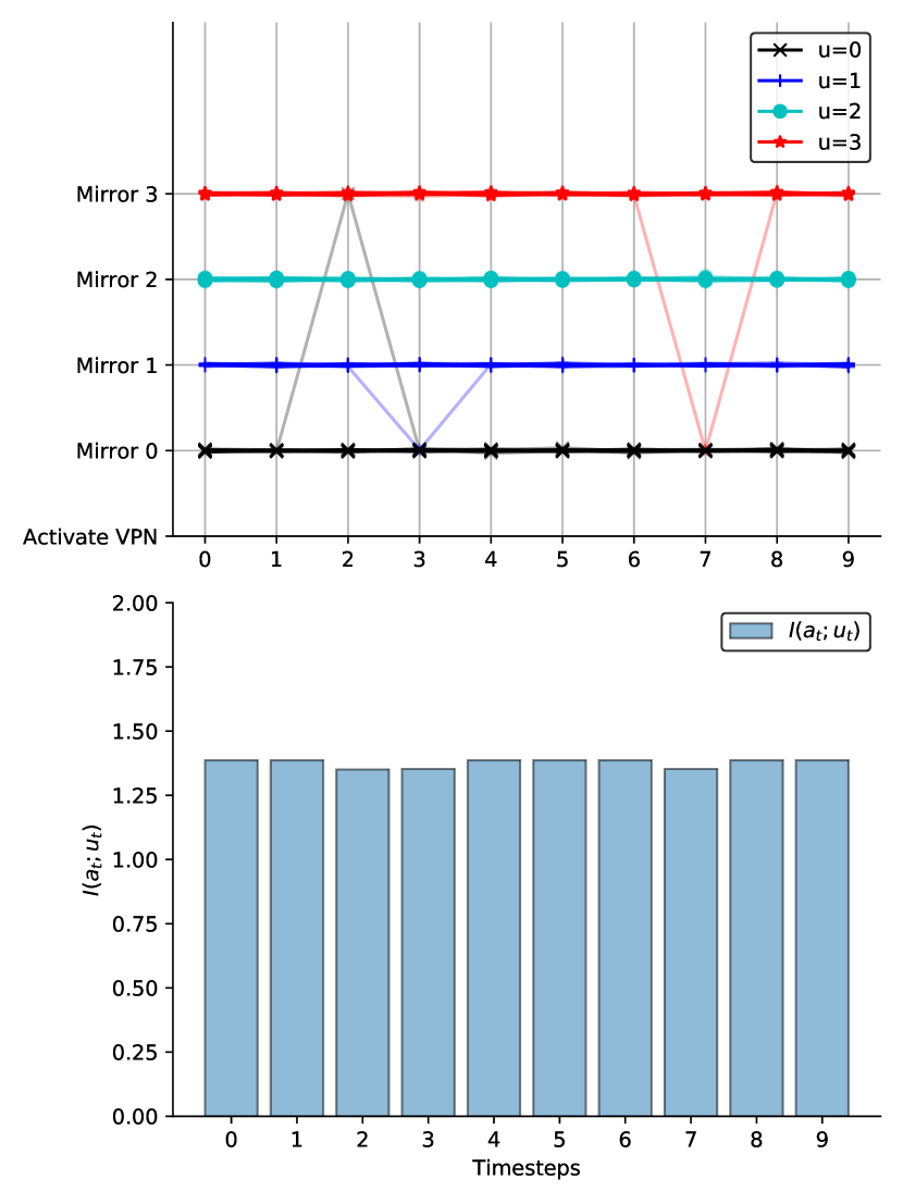
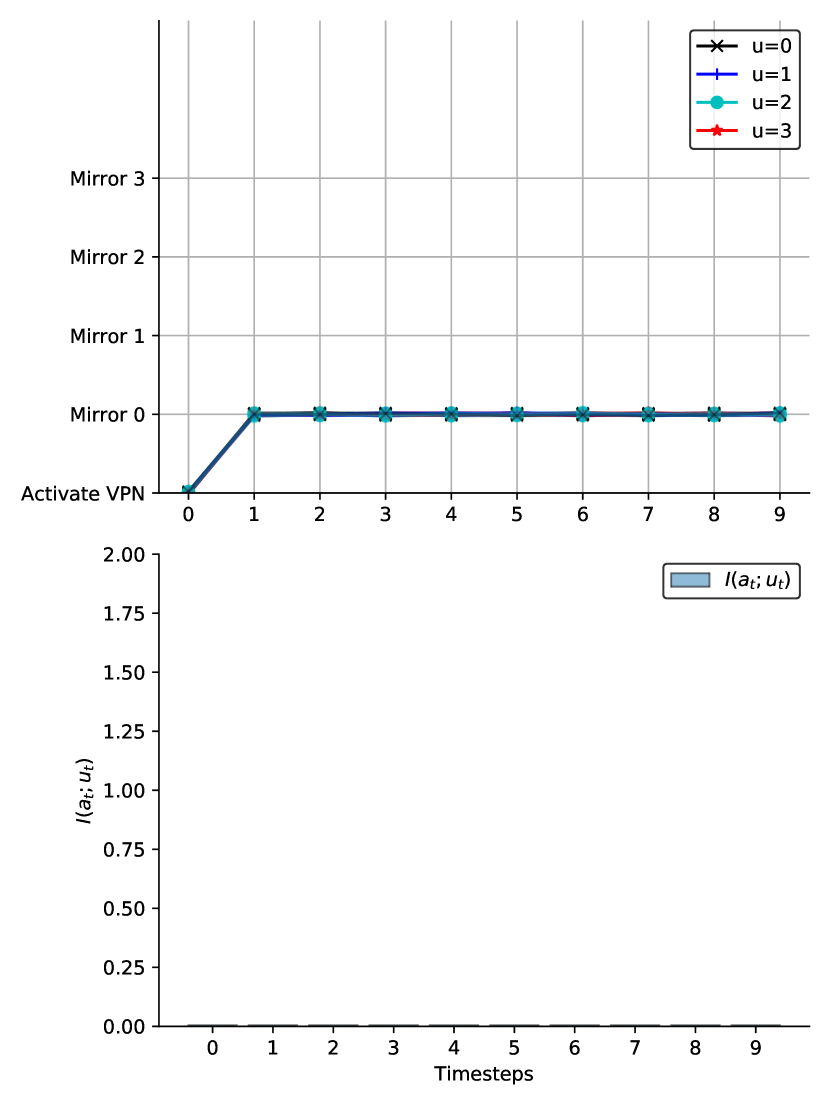
Figure 2: Trajectories from the internet connectivity environment. One the left we have a Lagrange multiplier $\boldsymbol{\lambda}=\boldsymbol{0}$, while on the right we have $\boldsymbol{\lambda}=\boldsymbol{1}$. We see that the trajectories in the constrained case are able to completely remove the mutual information between the action and the sensitive state by choosing a policy of always activating the VPN and then choosing mirror 0.

A.3.2 Controlling Individual Timesteps’ Mutual Information

We consider an idealized customer-service problem. In this problem, our agent controls a personalized goods distribution system, delivering goods to a specific person. The person has a location $x\in\mathbb{R}$, obeying a random walk where $x_{t+1}=x_{t}+\epsilon$, for $\epsilon\sim\mathcal{N}(0,\sigma^{2})$, and the agent has a ‘service center’ which is on a lattice $w\in\mathbb{Z}$ of possible locations from which deliveries are sent out. At each timestep, the agent is told the location of the person, and updates the location of its service center, either increasing it by 1 or decreasing it by 1. The agent then receives reward $r(x_{t},a_{t},w_{t})=-|x_{t}-w_{t}|$, being penalized for how far the service center is from the person. To make this a privacy-constrained problem, we suppose that there is an underlying sensitive binary variable $u\in\{0,1\}$, which heavily influences the initial position of the client. The sensitive variable $u$ is constant over the episode. In particular, we choose $p(x_{1},u)$ as $p(u)p(x_{1}|u)$ with $u\sim\text{Uniform}\ \{0,1\}$, $x\sim\mathcal{N}(2u,\sigma_{0}^{2})$. For our experiments we used $\sigma^{2}=1/4$ and $\sigma_{0}^{2}=0.5$. Since this environment is $u$-shielded per our definition in the appendix A.8, where $u$ also impacts the dynamics, with the update $x_{t+1}=x_{t}+u\alpha+\epsilon$. We used $\alpha=0.3$ in cases where we use this variant.

A.3.3 Results

Customer Service The results of the customer service experiments are shown in figures 3, 4. The experiments using the model-based estimator in equation 36 in figure 3 show that the model-based method is indeed able to selectively constrain the value of $I(u;a_{t})$ by choosing the right lagrange multipliers in equation 4. The trajectories match the intuitive expectations of the constraints: the unconstrained agent draws the trajectories as close to zero as quickly as possible to maximize reward. However the constrained agent is not able to do this, as it would reveal the protected variable. The agent that is heavily constrained on the first timestep moves both groups down, even though this results in less reward for the blue group: once at a timestep where it isn’t constrained, it moves both groups back towards zero.

We also present the model-free approach in figure 4, evaluating on the non-$u$-shielded version of the customer service example. Although harder to interpret the behaviour due to the global nature of the constraint over the whole sequence of actions, we see that the constrained agent takes a similar approach in choosing similar distributions of actions for both groups, while drawing the two groups gradually closer to the origin. Again, the unconstrained agent simply draws both groups to the origin immediately. Examining the trajectory-level mutual information, we see that the constrained agent has $I(u;\tau_{a},\tau_{x})\approx 0.35$, while for the unconstrained agent it is approximately $0.45$.

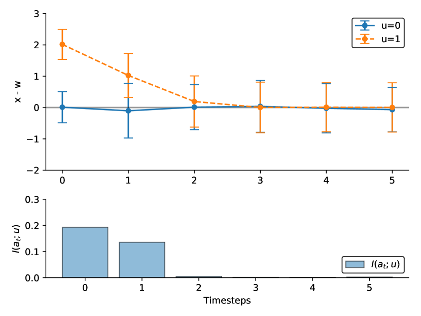
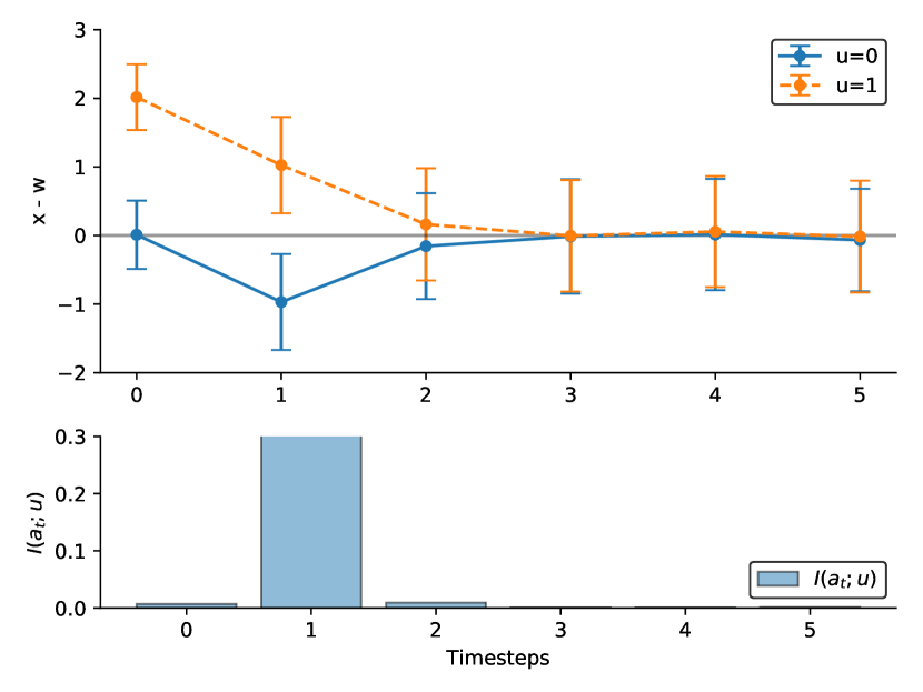
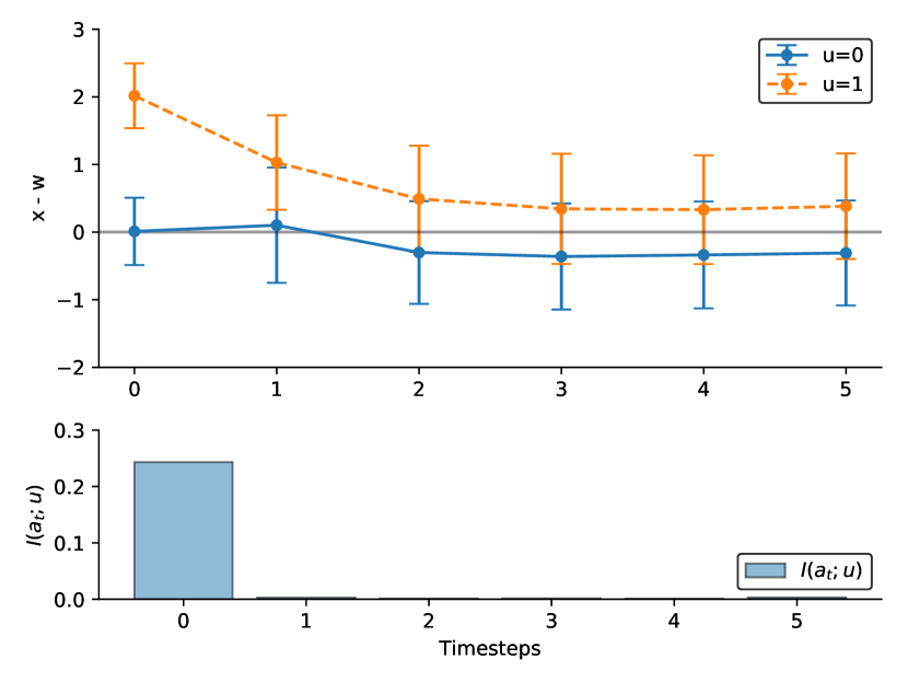
Figure 3: Trajectories and values of $I(a_{t};u)$ generated from different choices of Lagrange multipliers in equation 4 on the customer service problem, for the two different protected groups. The left shows $\boldsymbol{\lambda}=\boldsymbol{0}$, the middle shows $\boldsymbol{\lambda}=(10,0,\ldots,0)$, and the right shows $\boldsymbol{\lambda}=(0,10,\ldots,10)$. We get precise control over $I(a_{t};u)$ with the choices of $\boldsymbol{\lambda}$. For example, in the middle trajectory we see that a large Lagrange multiplier on the first timestep’s constraint forces the agent to treat both groups exactly the same, even at the expense of reward by moving away from zero. Once the constraint is removed, the agent exposes a large amount of information about the protected groups with its subsequent action.

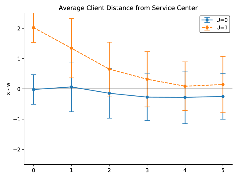
Figure 4: Trajectories induced by an agent trained against the model-free upper bound constraint. The trajectories are harder to interpret than when trained against the model-based constraint.

A.4 SNAP Allocation

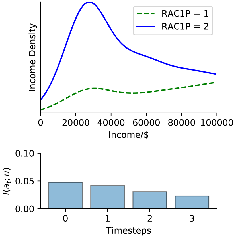
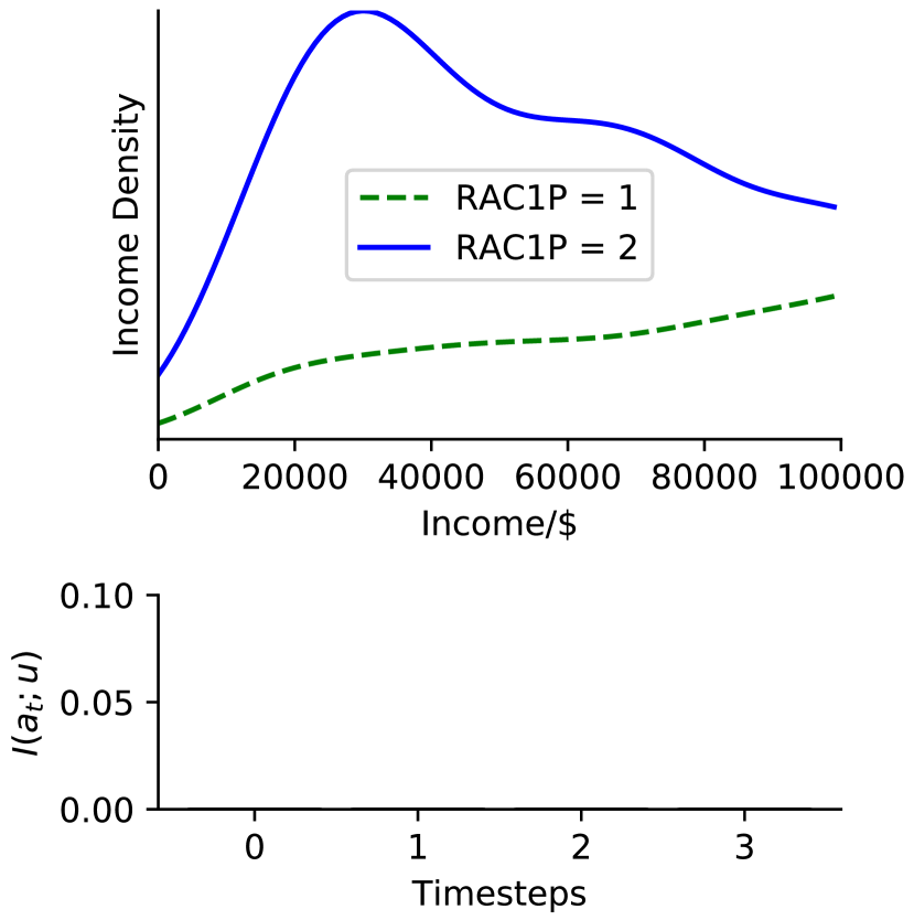
Figure 5: Final income distributions from privacy-constrained (right) and unconstrained (left) policies on the SNAP setting. The constrained policy removes all action-protected-variable mutual information.

To investigate the possibility of applications in algorithmic fairness, we implement a more realistic experiment using the supplemental nutrition assistance program (SNAP) data from the American Community Survey (ACS) microdata. For simplicity, we restrict our attention to households from Washington D.C., and to people who recorded their race under the ‘RAC1P’ code as ‘1’ or ‘2’, corresponding to White alone and Black or African American Alone. This resulted in 5,304 records, of which 2,933 were white and 2,371 black. Using these data, we then form a kernel density estimator of the income distribution of both race codes. The agent has a binary action, to either give SNAP or not. The next timestep is imagined to happen a year later. The person’s income is $x_{t}=x_{t-1}+\epsilon$ in the case where SNAP isn’t given (where $\epsilon\sim\mathcal{N}(0,\sigma^{2})$), and in the case where SNAP is given the income is $x_{t}=x_{t-1}+\epsilon+\gamma$, with $\gamma\sim\text{Uniform}(1512,7200)$. This $\gamma$ represents the increase in income due to the SNAP program, where the minimum and maximum limits correspond to the upper and lower bounds of SNAP contribution (Fang et al., 2019). We chose $\sigma=$ $1000. We treat the race variable as protected, and the income variable as unprotected. The reward at each timestep is $-\min\{0,L-x_{t}\}^{2}$, where $L$ is the federal poverty level of $24,900.

Results: As we can see in figure 5, we are able to reduce the mutual information exposed by the policy’s actions while not changing the final income distribution unduly. In the unconstrained case there is a noticeable peak around the poverty level as the policy strictly gives assistance to those below and not above. The constrained case shows a gentler increase corresponding to a stochastic policy that is limited in the extent to which it can use the sensitive race variable (which is correlated to income). As discussed in section 3, careful consideration of the societal impacts of using this independence measure as a fairness benchmark is required.

A.5 Comparison to Differentially-Private Q-Learning

Figure 6 shows the action distribution for our approach, compared to the DPQL approach. We show the four states corresponding to $u\in\{0,1\}$ in the VPN example with four mirrors. The states with $u\in\{2,3\}$ are similar and omitted to make the plot clearer. We see that the DPQL approach works through adding noise to the $Q$-values, while our approach takes into account the feedback in the MDP, choosing the VPN at the first timestep.

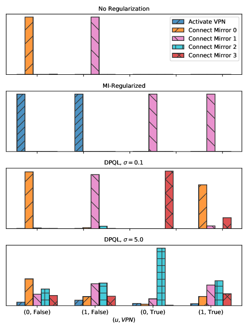
Figure 6: Distribution of actions in four states in the VPN example with four mirrors. From top to bottom, we have our approach with $\boldsymbol{\lambda}=0$, our approach with $\boldsymbol{\lambda}=1$, DPQL with $\sigma=0.1$, and $\sigma=5.0$

A.6 Full Algorithm

For completeness we give the full algorithmic details here. This pseudocode is very close to the actual implementation.

Algorithm 3 Model-Based MI-Constrained Policy Gradients

  Input: Vector $\boldsymbol{\epsilon_{t}}\in\mathbb{R}_{\geq 0}^{T}$, number of $\psi$ gradient steps $n$, number of $\phi$ gradient steps $m$, gradient-based optimization method step, batch size $B$, model $p$.

  Initialize Lagrange multipliers $\boldsymbol{\lambda}\in\mathbb{R}_{\geq 0}^{T}$, initial policy, discriminator and baseline parameters $\phi,\psi_{1:T},\theta$

  while min over $\boldsymbol{\lambda}$ not converged do

     Change $\boldsymbol{\lambda}$ by coordinate descent

     while inner max-min over $\psi,\phi$ not converged do

        for i = 1, …, $n$ do

           Draw batch $\tau_{1:B}\sim q_{\phi}(\tau)$

           for $t=1,\ldots,T$ do

              $g_{\psi,t}=\nabla_{\psi}\tfrac{1}{B}\sum_{j=1}^{B}\log q_{\psi}(\tau_{u,j}|\tau_{a,j,t})$

              $\psi_{t}=\mathtt{step}(\psi_{t},g_{\psi,t})$

           end for

        end for

        for i = 1, …, $m$ do

           Draw batch $\tau_{1:B}\sim q_{\phi}(\tau)$

           $w,r,g,g^{\prime}=\mathtt{zeros}(T)$, $g_{1},g_{2}^{\prime},g_{\theta}=0$

           for $\tau\in\tau_{1:B}$ do

              for t = 1, …, $T$ do

                 $x_{t}=\tau_{x,t},\ a_{t}=\tau_{a,t},\ u_{t}=\tau_{u,t}$

                 $v=\int_{a^{\prime}_{t}}q(a^{\prime}_{t}|x_{t},u_{t})p(x_{t+1}|a^{\prime}_{t},x_{t},u_{t})$

                 $g_{t}=\nabla_{\phi}\left[\log q_{\phi}(a_{t}|x_{t},u)\right]$

                 $w_{t}=g_{t}p(x_{t+1}|a_{t},x_{t},u_{t})/v$

                 $r_{t}=\log q_{\psi}(u_{t}|a_{t})-\log p(u_{t})$

                 $A_{t}=\left[\sum_{t^{\prime}=t}^{T}r(x_{t^{\prime}},a_{t^{\prime}},u_{t^{\prime}})\right]-\theta(x_{t},u_{t})$

                 $g_{2}^{\prime}=g_{2}^{\prime}+g_{t}A_{t}$

                 $g_{\theta}^{\prime}=g_{\theta}^{\prime}+\nabla_{\theta}\left[(\theta(x_{t},u_{t})-A_{t})^{2}\right]$

              end for

              $g^{\prime}_{1}=g^{\prime}_{1}+r_{t}\left(g_{t}+\sum_{t^{\prime}=1}^{t-1}w_{t^{\prime}}\right)$

           end for

           $g_{1}=\tfrac{1}{B}\sum_{t=1}^{T}g^{\prime}_{1}$, $g_{2}=\tfrac{1}{BT}\sum_{t=1}^{T}g^{\prime}_{2}$

           $\phi=\mathtt{step}(\phi,g_{1}+g_{2})$, $\theta=\mathtt{step}(\theta,\frac{1}{BT}g^{\prime}_{\theta})$

        end for

     end while

  end while

Algorithm 4 Model-Free MI-Constrained Policy Gradients

  Input: Constraint $\epsilon\geq 0$, number of $\psi$ gradient steps $n$, number of $\phi$ gradient steps $m$, gradient-based optimization update step, batch size $B$

  Initialize Lagrange multipliers $\lambda\in\mathbb{R}_{\geq 0}^{T}$, initial policy, discriminator and baseline parameters $\phi,\psi,\theta$

  while min over $\lambda$ not converged do

     Change $\lambda$ by coordinate descent

     while inner max-min over $\psi,\phi$ not converged do

        for i = 1, …, $n$ do

           Draw batch $\tau_{1:B}\sim q_{\phi}(\tau)$

           for j = 1, …, $B$ do

              $g_{\psi}=g_{\psi,t}+\nabla_{\psi}\log q_{\psi}(\tau_{u,j}|\tau_{a,j},\tau_{x,j})$

           end for

           $\psi=\mathtt{step}(\psi,\tfrac{1}{B}g_{\psi})$

        end for

        for i = 1, …, $m$ do

           Draw batch $\tau_{1:B}\sim q_{\phi}(\tau)$

           $w,r,g,g^{\prime}=\mathtt{zeros}(T)$, $g_{1},g_{2}^{\prime},g_{\theta}^{\prime}=0$.

           for $\tau\in\tau_{1:B}$ do

              for t = 1, …, $T$ do

                 $\boldsymbol{x}_{t}=\tau_{x,t},\ a_{t}=\tau_{a,t},\ \boldsymbol{u}_{t}=\tau_{u,t}$

                 $g_{t}=\nabla_{\phi}\left[\log q_{\phi}(a_{t}|x_{t},u_{t},)\right]$

                 $A_{t}=\left[\sum_{t^{\prime}=t}^{T}r(x_{t^{\prime}},a_{t^{\prime}},u_{t^{\prime}})\right]-\theta(x_{t},u_{t})$

                 $g_{2}^{\prime}=g_{2}^{\prime}+g_{t}A_{t}$

                 $g_{\theta}^{\prime}=g_{\theta}^{\prime}+\nabla_{\theta}\left[(\theta(x_{t},u_{t})-A_{t})^{2}\right]$

              end for

              $g_{1}=g_{1}+\frac{\log q_{\psi}(\tau_{u}|\tau_{a},\tau_{x})}{\log p(\tau_{u})}\sum_{t=1}^{T}g_{t}$

           end for

           $g_{1}=\tfrac{1}{B}\sum_{t=1}^{T}g^{\prime}_{1}$, $g_{2}=\tfrac{1}{BT}\sum_{t=1}^{T}g^{\prime}_{2}$

           $\phi=\mathtt{step}(\phi,g_{1}+g_{2})$, $\theta=\mathtt{step}(\theta,\frac{1}{BT}g^{\prime}_{\theta})$

        end for

     end while

  end while

A.7 Additional Experimental Details

All experiments were run on a dual-core 3.5GHz Intel i7 CPU, with the runs taking around one minute to complete. We selected the hyperparameters by hand, observing which ones resulting in convergence. In the case of the Lagrange multipliers $\lambda$, we tried a few different settings to see which was best for equation (4). For all experiments we used the Adam optimizer (Kingma & Ba, 2015) for all gradient-based optimization.

A.7.1 Internet Connectivity Example

Hyperparameter	Value
$r^{*}$	1.
$r^{-}$	0.5
$r^{\text{VPN}}$	0.9
T	10
Batch Size	32
Number of Epochs	5000
Learning Rate	3$\cdot 10^{-3}$

Table 1: Internet Connectivity Hyperparameters

Hyperparameter	Value
Environment Force Noise $\sigma$	0.5
Initial Position $\sigma$	1.
$r^{\text{VPN}}$	0.9
T	10
Batch Size	128
Number of Epochs	4000
Learning Rate	3$\cdot 10^{-3}$

Table 2: 2d Control Hyperparameters

Hyperparameter	Value
Income KDE Bandwidth	$10,000
T	4
Batch Size	128
Number of Epochs	1000
Learning Rate	1$\cdot 10^{-3}$

Table 3: SNAP Hyperparameters

Hyperparameter	Value
Initial Separation	2
Dynamics Noise $\sigma$	0.25
Initial Distribution $\sigma$	0.5
T	6
Batch Size	12
Number of Epochs	5000
Learning Rate	1$\cdot 10^{-4}$

Table 4: Customer Service Hyperparameters

A.8 Upper Bound Loosesness with Shielded $u$.

If we are completely unable to form a dynamics estimator we may use $I_{q}(\tau_{a},\tau_{x};\tau_{u})$ to constrain $I_{q}(a_{t};u_{t})$. However, there is a significant class of problems for which the upper bound is loose, which we call $u$-shielded MDPs.

Figure 7:

Figure 8: A $u$-shielded MDP

They have the property where the protected variable $u$ influences the initial distribution, but subsequently $u$ doesn’t directly influence the dynamics or the rewards of the MDP. An idealised example would be a banking system where minority status influences initial income distribution, but (conditioned on income) the default rate doesn’t depend on minority status, and the banking system’s performance is evaluated without reference to minority status. In that case the policy $q(a|x,u)$ doesn’t need to depend on $u$ at all, in the sense that for any policy $q(a|x,u)$ there is another policy $q(a|x,u)=q(a|x)p(u)$ with the same reward. Hence without loss of generality we assume that all policies in the $u$-shielded setting are in this $u$-independent form.

In that case, we have that

Lemma A.1.

In a $u$-shielded MDP, and a greedy policy $q_{\text{greedy}}$ which is reward-maximizing under no mutual information constraint, $I_{q}(\tau_{x},\tau_{a};u)\geq I_{q_{\text{greedy}}}(a_{t};u)$ for any policy $q$.

Proof.

We have $I_{q}(\tau_{x},\tau_{a};u)=\sum_{t=1}^{T}I_{q}(x_{t},a_{t};u|\tau_{a_{1:t}},\tau_{x_{1:t}})=I_{q}(x_{1};u)$, by the decomposition of mutual information and the fact that $x_{t}$ and $a_{t}$ are conditionally independent from $u$ given $x_{1}$. The data processing inequality on the Markov chain $u\rightarrow x_{1}\rightarrow a_{t}$ gives us $I_{\text{greedy}}(a_{t};u)\leq I_{p}(x_{1};u)$. Therefore, we have $I_{\text{greedy}}(a_{t};u)\leq I_{q}(\tau_{x},\tau_{a};u)$. ∎

In particular, this result tells us that if we constrain our upper bound in the hope of reducing $I(a_{t};u)$, if our problems have the $u$-shielded property then our constraint will never exclude the greedy policy.

A.9 Equivalence to Demographic Parity in Single-Timestep Case

By writing the binary classification problem with a demographic parity constraint as an RL problem, we can show its equivalence to our privacy constraint in the single-timestep case. Since classification has no concept of feedback, we can describe the demographic parity constrained classification problem as an episodic MDP with only one timestep. We define the MDP-classification setting as the MDP with $T=1$, action space $\mathcal{A}=\{0,1\}$ corresponding to the two possible labels, state space $\mathcal{X}\times\mathcal{U}$, and a reward distribution $r(x_{1},u_{1},a_{1})=-\mathds{1}\left[a_{1}=y\right]$ for random variable $y\sim p(y|x_{1},u_{1})$ (for $\mathcal{Y}=\{0,1\}$) corresponding to 0-1 loss.

Lemma A.2.

Problem (2) with the MDP-classification setting is equivalent to the fair classification problem with the 1-0 loss and the generalised demographic parity (DP) fairness constraint ($I(\hat{y};u)<\epsilon$) for all $p(x,u,y)$. Furthermore, the mutual information constraint in equation (2) is the only choice of constraint with this equivalence.

Proof.

To solve problem (2) with the specified dynamics requires finding a policy $q(a_{1}|x_{1},u_{1})$ that maximizes $\mathbb{E}_{a_{1},x_{1},u_{1},y\sim q(a_{1},x_{1},u_{1},y)}\left[\mathds{1}\left[a_{1}=y\right]\right]$, subject to $I(u_{1};a_{1})<\epsilon$. Solving the fair classification problem with demographic parity requires learning a model that emits a classification $\hat{Y}$ maximizing $\mathbb{E}_{\mathbf{x},\mathbf{u},Y\sim p(\mathbf{x},\mathbf{u},Y)}\left[\mathds{1}\left[\hat{Y}=Y\right]\right]$ subject to $I(\hat{Y};\mathbf{u})<\epsilon$. Hence we have the same objective, and so the problems are the same if and only if they have the same constraints, i.e. we have the constraint $I(a_{1};u_{1})$. ∎

References

- A. & Fu (2018) A., P. L. and Fu, M. Risk-Sensitive Reinforcement Learning: A Constrained Optimization Viewpoint. arXiv:1810.09126 [cs, math, stat], October 2018.
- Agarwal & Singh (2017) Agarwal, N. and Singh, K. The price of differential privacy for online learning. In Proceedings of the 34th International Conference on Machine Learning - Volume 70, ICML’17, pp. 32–40, Sydney, NSW, Australia, August 2017. JMLR.org.
- Altman (1999) Altman, E. Constrained Markov Decision Processes. Stochastic Modeling. Chapman & Hall/CRC, Boca Raton ; London, 1999. ISBN 978-0-8493-0382-1.
- Anderson (1988) Anderson, M. J. The American Census: A Social History. Yale Univ. Press, New Haven, 3rd edition, 1988. ISBN 978-0-300-04709-7. OCLC: 255721580.
- Basu et al. (2019) Basu, D., Dimitrakakis, C., and Tossou, A. Differential privacy for multi-armed bandits: What is it and what is its cost? arXiv preprint arXiv:1905.12298, 2019.
- Bradbury et al. (2020) Bradbury, J., Frostig, R., Hawkins, P., Johnson, M. J., Leary, C., Maclaurin, D., and Wanderman-Milne, S. JAX: Composable transformations of Python+NumPy programs}, 2020.
- Dalal et al. (2018) Dalal, G., Dvijotham, K., Vecerik, M., Hester, T., Paduraru, C., and Tassa, Y. Safe Exploration in Continuous Action Spaces. arXiv:1801.08757 [cs], January 2018.
- Du et al. (2019) Du, S. S., Kakade, S. M., Wang, R., and Yang, L. F. Is a Good Representation Sufficient for Sample Efficient Reinforcement Learning? arXiv:1910.03016 [cs, math, stat], October 2019.
- du Pin Calmon & Fawaz (2012) du Pin Calmon, F. and Fawaz, N. Privacy against statistical inference. In 2012 50th Annual Allerton Conference on Communication, Control, and Computing (Allerton), pp. 1401–1408, October 2012. doi: 10.1109/Allerton.2012.6483382.
- Dwork et al. (2006) Dwork, C., McSherry, F., Nissim, K., and Smith, A. Calibrating Noise to Sensitivity in Private Data Analysis. In Halevi, S. and Rabin, T. (eds.), Theory of Cryptography, Lecture Notes in Computer Science, pp. 265–284, Berlin, Heidelberg, 2006. Springer. ISBN 978-3-540-32732-5. doi: 10.1007/11681878_14.
- Fang et al. (2019) Fang, B., Jiang, M., Shen, J., Cheng, P.-Y., and Chivukula, M. Food Fairness: An Artificial Intelligence Perspective for SNAP Allocation. Workshop on AI for Social Good, IJCAI, pp. 5, 2019.
- Gauci et al. (2019) Gauci, J., Conti, E., Liang, Y., Virochsiri, K., He, Y., Kaden, Z., Narayanan, V., Ye, X., Chen, Z., and Fujimoto, S. Horizon: Facebook’s Open Source Applied Reinforcement Learning Platform. arXiv:1811.00260 [cs, stat], September 2019.
- Goyal et al. (2019) Goyal, A., Islam, R., Strouse, D., Ahmed, Z., Botvinick, M., Larochelle, H., Levine, S., and Bengio, Y. InfoBot: Transfer and Exploration via the Information Bottleneck. arXiv preprint arXiv:1901.10902, 2019.
- Haarnoja et al. (2018) Haarnoja, T., Zhou, A., Abbeel, P., and Levine, S. Soft Actor-Critic: Off-Policy Maximum Entropy Deep Reinforcement Learning with a Stochastic Actor. In International Conference on Machine Learning, pp. 1856–1865, 2018.
- Higgins et al. (2017) Higgins, I., Pal, A., Rusu, A., Matthey, L., Burgess, C., Pritzel, A., Botvinick, M., Blundell, C., and Lerchner, A. DARLA: Improving zero-shot transfer in reinforcement learning. In Proceedings of the 34th International Conference on Machine Learning-Volume 70, pp. 1480–1490, 2017.
- Jabbari et al. (2017) Jabbari, S., Joseph, M., Kearns, M., Morgenstern, J., and Roth, A. Fairness in reinforcement learning. In Proceedings of the 34th International Conference on Machine Learning-Volume 70, pp. 1617–1626. JMLR. org, 2017.
- Kaiser et al. (2019) Kaiser, L., Babaeizadeh, M., Milos, P., Osinski, B., Campbell, R. H., Czechowski, K., Erhan, D., Finn, C., Kozakowski, P., Levine, S., Mohiuddin, A., Sepassi, R., Tucker, G., and Michalewski, H. Model-Based Reinforcement Learning for Atari. arXiv:1903.00374 [cs, stat], March 2019.
- Kingma & Ba (2015) Kingma, D. P. and Ba, J. Adam: A method for stochastic optimization. International Conference on Learning Representations, 2015.
- Liao et al. (2017) Liao, J., Sankar, L., Calmon, F. P., and Tan, V. Y. F. Hypothesis testing under maximal leakage privacy constraints. In 2017 IEEE International Symposium on Information Theory (ISIT), pp. 779–783, June 2017. doi: 10.1109/ISIT.2017.8006634.
- Mir (2012) Mir, D. J. Information-Theoretic foundations of differential privacy. In Proceedings of the 5th International Conference on Foundations and Practice of Security, FPS’12, pp. 374–381, Berlin, Heidelberg, October 2012. Springer-Verlag. ISBN 978-3-642-37118-9. doi: 10.1007/978-3-642-37119-6_25.
- Mishra & Thakurta (2015) Mishra, N. and Thakurta, A. (Nearly) optimal differentially private stochastic multi-arm bandits. In Proceedings of the Thirty-First Conference on Uncertainty in Artificial Intelligence, UAI’15, pp. 592–601, Arlington, Virginia, USA, July 2015. AUAI Press. ISBN 978-0-9966431-0-8.
- Nabi et al. (2019) Nabi, R., Malinsky, D., and Shpitser, I. Learning Optimal Fair Policies. Proceedings of machine learning research, 97:4674–4682, June 2019. ISSN 2640-3498.
- Neel & Roth (2018) Neel, S. and Roth, A. Mitigating bias in adaptive data gathering via differential privacy. In International Conference on Machine Learning, pp. 3720–3729, 2018.
- Nowozin et al. (2016) Nowozin, S., Cseke, B., and Tomioka, R. F-gan: Training generative neural samplers using variational divergence minimization. In Advances in Neural Information Processing Systems, pp. 271–279, 2016.
- Paninski (2003) Paninski, L. Estimation of Entropy and Mutual Information. Neural Computation, 15(6):1191–1253, June 2003. ISSN 0899-7667, 1530-888X. doi: 10.1162/089976603321780272.
- Papamakarios et al. (2019) Papamakarios, G., Nalisnick, E., Rezende, D. J., Mohamed, S., and Lakshminarayanan, B. Normalizing Flows for Probabilistic Modeling and Inference. arXiv:1912.02762 [cs, stat], December 2019.
- Sajed & Sheffet (2019) Sajed, T. and Sheffet, O. An Optimal Private Stochastic-MAB Algorithm Based on an Optimal Private Stopping Rule. arXiv:1905.09383 [cs, stat], May 2019.
- Sakuma et al. (2008) Sakuma, J., Kobayashi, S., and Wright, R. N. Privacy-preserving reinforcement learning. In Proceedings of the 25th International Conference on Machine Learning - ICML ’08, pp. 864–871, Helsinki, Finland, 2008. ACM Press. ISBN 978-1-60558-205-4. doi: 10.1145/1390156.1390265.
- Shariff & Sheffet (2018) Shariff, R. and Sheffet, O. Differentially private contextual linear bandits. In Proceedings of the 32nd International Conference on Neural Information Processing Systems, NIPS’18, pp. 4301–4311, Red Hook, NY, USA, December 2018. Curran Associates Inc.
- Silver et al. (2016) Silver, D., Huang, A., Maddison, C. J., Guez, A., Sifre, L., van den Driessche, G., Schrittwieser, J., Antonoglou, I., Panneershelvam, V., Lanctot, M., Dieleman, S., Grewe, D., Nham, J., Kalchbrenner, N., Sutskever, I., Lillicrap, T., Leach, M., Kavukcuoglu, K., Graepel, T., and Hassabis, D. Mastering the game of Go with deep neural networks and tree search. Nature, 529(7587):484–489, January 2016. ISSN 0028-0836, 1476-4687. doi: 10.1038/nature16961.
- Smith & Thakurta (2013) Smith, A. and Thakurta, A. (Nearly) optimal algorithms for private online learning in full-information and bandit settings. In Proceedings of the 26th International Conference on Neural Information Processing Systems - Volume 2, NIPS’13, pp. 2733–2741, Red Hook, NY, USA, December 2013. Curran Associates Inc.
- Song et al. (2019) Song, J., Kalluri, P., Grover, A., Zhao, S., and Ermon, S. Learning Controllable Fair Representations. Proceedings of the 22nd International Conference on Artificial Intelligence and Statistics (AISTATS), 2019.
- Strouse et al. (2018) Strouse, D. J., Kleiman-Weiner, M., Tenenbaum, J., Botvinick, M., and Schwab, D. J. Learning to share and hide intentions using information regularization. In Advances in Neural Information Processing Systems, pp. 10249–10259, 2018.
- Sutton & Barto (2018) Sutton, R. S. and Barto, A. G. Reinforcement Learning: An Introduction. Adaptive Computation and Machine Learning Series. The MIT Press, Cambridge, Massachusetts, second edition, 2018. ISBN 978-0-262-03924-6.
- Tossou & Dimitrakakis (2016) Tossou, A. C. Y. and Dimitrakakis, C. Algorithms for differentially private multi-armed bandits. In Proceedings of the Thirtieth AAAI Conference on Artificial Intelligence, AAAI’16, pp. 2087–2093, Phoenix, Arizona, February 2016. AAAI Press.
- van Dijk & Polani (2011) van Dijk, S. G. and Polani, D. Grounding subgoals in information transitions. In 2011 IEEE Symposium on Adaptive Dynamic Programming and Reinforcement Learning (ADPRL), pp. 105–111, April 2011. doi: 10.1109/ADPRL.2011.5967384.
- Vietri et al. (2020) Vietri, G., Balle, B., Krishnamurthy, A., and Wu, Z. S. Private reinforcement learning with PAC and regret guarantees. International Conference on Machine Learning, 2020.
- Wang & Hegde (2019) Wang, B. and Hegde, N. Privacy-preserving Q-Learning with Functional Noise in Continuous State Spaces. In Advances in Neural Information Processing Systems, 2019.
- Wang et al. (2016) Wang, W., Ying, L., and Zhang, J. On the Relation Between Identifiability, Differential Privacy, and Mutual-Information Privacy. IEEE Transactions on Information Theory, 62(9):5018–5029, September 2016. ISSN 1557-9654. doi: 10.1109/TIT.2016.2584610.
- Zemel et al. (2013) Zemel, R., Wu, Y., Swersky, K., Pitassi, T., and Dwork, C. Learning fair representations. In International Conference on Machine Learning, pp. 325–333, 2013.
- Zhang & Makedon (2005) Zhang, S. and Makedon, F. Privacy preserving learning in negotiation. In Proceedings of the 2005 ACM Symposium on Applied Computing, SAC ’05, pp. 821–825, New York, NY, USA, March 2005. Association for Computing Machinery. ISBN 978-1-58113-964-8. doi: 10.1145/1066677.1066865.