The homotopy type of the contactomorphism groups of tight contact $3$-manifolds, part I

Abstract.

We compute the homotopy type of the space of embeddings of convex disks with Legendrian boundary into a tight contact $3$-manifold, whenever the sum of the absolute value of the rotation number of the boundary with the Thurston-Bennequin invariant is $-1$, proving that it is homotopy equivalent to the space of smooth embeddings. Using the same ideas it is also determined the homotopy type of the space of embeddings of convex spheres into a tight $3$-fold in terms of the space of smooth spheres. As a consequence we determine the homotopy type of the space of long Legendrian unknots, satisfying the previous condition, into a tight $3$-fold and also of the space of long transverse unknots with self-linking number $-1$, proving that these spaces are homotopy equivalent to the space of smooth long unknots. We also determine the homotopy type of the contactomorphism group of every universally tight handlebody, the standard ${\mathbb{S}}^{1}\times{\mathbb{S}}^{2}$ and every Legendrian fibration over a compact orientable surface with non-empty boundary, partially solving a conjecture due to E. Giroux. Finally, we show that the space of embeddings of Legendrian $(n,n)$-torus links with maximal Thurston-Bennequin invariant is homotopy equivalent to $\operatorname{U}(2)\times K(\mathcal{M}_{n},1)$, where $\mathcal{M}_{n}$ is the mapping class group of the $2$-sphere with $n$-holes.

1. Introduction.

Throughout this article $M$ will be an oriented compact $3$-manifold and $\xi$ a positive contact structure on $M$, that we will always assume cooriented. The pair $(M,\xi)$ is a contact $3$-manifold. A remarkable fact, due to Gray [Gra59], is that there are no trivial deformations of contact structures on $M$: every homotopy $\xi_{t}$, $t\in[0,1]$, of contact structures is generated by a flow $\varphi_{t}\in\operatorname{Diff}_{0}(M)$. Here, $\operatorname{Diff}_{0}(M)$ denotes the path–connected component of the identity in $\operatorname{Diff}(M)$, the orientation preserving diffeomorphism group of $M$. Therefore, the topology of the space ${\mathfrak{C}Str}(M,\xi)$ of contact structures on $M$ homotopic to $\xi$, is locally uninteresting. However, the global topology of this space could contain interesting information, depending on the underlying manifold $M$ or even on the isomorphism class of the contact structure $\xi$. Gray stability result works parametrically giving rise to a fiber bundle:

$$\operatorname{Cont}_{0}(M,\xi)\hookrightarrow\operatorname{Diff}_{0}(M)\rightarrow{\mathfrak{C}Str}(M,\xi)$$

called the Gray Fibration. The fiber $\operatorname{Cont}_{0}(M,\xi)$ is conformed by those diffeomorphisms that preserve $\xi$ and are smoothly isotopic to the identity. Diffeomorphisms satisfying the first property are known as contactomorphisms and they conform the group $\operatorname{Cont}(M,\xi)$ of contactomorphisms of $(M,\xi)$. In this article, we will use topological methods to study the group $\operatorname{Cont}(M,\xi)$ of contactomorphisms of $(M,\xi)$ or, almost equivalently, the space of contact structures ${\mathfrak{C}Str}(M,\xi)$. For us, the diffeomorphism group of $M$ is an input. We do note that in the case with non-empty boundary we always assume that the diffeomorphisms/contactomorphisms are the identity on an open neighbourhood of the boundary and also that all the contact structures do coincide over an open neighbourhood of the boundary. The same type of consideration will apply when speaking about embeddings of submanifolds with boundary.

Since the appearance of Hatcher’s proof of the Smale Conjecture [Hat83], there has been a big development in our understanding of the homotopy type of the diffeomorphism group of a $3$-manifold $M$ [BK17, BK21, Gab01, HKMR12, HL84]. The analog of the Smale Conjecture in contact topology is Eliashberg-Mishachev contractibility result of the contactomorphism group of the standard $3$-disk [EM21]. This result suggests that $3$-dimensional contact topology could be “closer” to smooth topology than “expected”. However, our understanding of the contactomorphism group of a contact manifold is not as good as in the smooth case. The reason being that the usual cut and paste ideas used to understand the diffeomorphism group are difficult to adapt to the contact setting since one needs to fix the germ of the contact structure over families of submanifolds to being able to apply the Contact Isotopy Extension Theorem. For low dimensional families of submanifolds (dimension 0 and 1) this is usually done by means of Giroux Convex Surface Theory [Gir91], which unfortunately, does not behave well parametrically. In this article we introduce a new method, based on the notion of microfibration introduced by Gromov [Gro86, Wei05], to deal with parametric families of surfaces with fixed characteristic foliation in a contact $3$-manifold. The idea is similar in spirit to Colin’s Discretization Trick [Col97]. We will apply this method in several cases in which it can be applied on the nose. As to apply Colin’s Trick effectively there are some requirements to apply this method that are not always satisfied.

Eliashberg-Mishachev Theorem is an h-principle type result [EM02, Gro86] for the contactomorphism group of the tight contact $3$-ball $(M,\xi)$. Recall that after the foundational work of Y. Eliashberg [Eli89, BEM15], there are two classes of contact $3$-manifolds: tight and overtwisted. While the second class is governed by an h-principle once one fixes a specific germ over a fixed disk, an overtwisted disk; the first ones were thought to have a rigid nature. In fact, this is the case at the $\pi_{0}$-level. It is important to note that the condition about the overtwisted disk being fixed is not vacuous: the space of overtwisted disks has topology strictly richer than the space of smooth disks in some cases [Vog18]. Apart from the work of Y.Chekanov and T. Vogel nothing is known about the space of overtwisted disks on a contact $3$-fold, thus nothing is known about the full contactomorphism group. In the other hand, we know everything of the subgroup of those which preserve an overtwisted disk [Dym01, Dym05].

On the tight case there has been a lot effort to classify tight contact structures. Loosely speaking the main tactic followed was to mimic the cut and paste techniques in smooth 3-dimensional topology and has two main steps [Hon02]: (i) Giroux Convex Surface Theory [Gir91] that allows to cut a contact 3-manifold along a surface and, even more important in some cases (the ones for which there is a classification type result) to have control over the germ of the contact structure over this surface. (ii) Finding a family of convex embedded disjoint surfaces $\Sigma_{i}$ inside the contact manifold $(M,\xi)$ in such a way $M\backslash(\cup\Sigma_{i})$ is contactomorphic to a finite union of tight balls, which are unique up to contactomorphism because of Eliashberg’s Classification result for the tight $3$-ball [Eli92]. Thus, the problem about understanding contact structures in dimension $3$ is reduced to understanding possible germs of contact structures over a family of surfaces in a fixed manifold. For the $\pi_{0}$-level, there is a stream of articles by Giroux, Colin, Honda, Kanda, Kazez, Mátic, etc; in which they provide a coarse classification of the space of contact structures [CGH09, Col97, Gir00, Gir01b, Gir01a, Yut97, Hon00a, Hon00b, HKM03]. There are also some articles dealing with the contact mapping class group as [Bou06, DG10, GM17, GGP04, GK14, Min22, ME21]. For higher dimensional manifolds much less is known but the reader can consult [CS16, CP14, FG20, Gir21, Gir19] for some partial results.

In general, there was not general path to approach the study the higher homotopy groups of the contactomorphism group of a tight contact $3$-manifold. We hope that this article could be a starting point in this research direction. In particular, we will provide several computations of the homotopy type of the contactomorphism group of several tight contact $3$-manifolds. These are the only known examples beyond the mentioned h-principle of [EM21]. We will follow the strategy explained above to classify tight contact structures in a parametric way, making use of our microfibration method to deal with parametric families of convex surfaces.

Let $(M,\xi)$ be a contact $3$-manifold. Let $e:{\mathbb{D}}^{2}\hookrightarrow(M,\xi)$ be a convex embedding bounding a Legendrian with $(\operatorname{tb},\operatorname{rot})=(t,r)$ such that $t+|r|=-1$. Let us denote by ${\mathfrak{Emb}}({\mathbb{D}}^{2},M)$ the space of embeddings of disks that coincide with $e$ over an open neighbourhood of the boundary $\partial{\mathbb{D}}^{2}$ and by ${\mathfrak{Emb}}_{\operatorname{std}}({\mathbb{D}}^{2},(M,\xi))$ the subspace of ${\mathfrak{Emb}}({\mathbb{D}}^{2},M)$ conformed by convex embeddings $j:{\mathbb{D}}^{2}\hookrightarrow(M,\xi)$ that have the same characteristic foliation than $e$, i.e. $j^{*}\xi=e^{*}\xi$. Then

Theorem 1.0.1 (Theorems 3.2.2 and 3.2.4).

Let $(M,\xi)$ be a tight contact $3$-manifold. Then, the natural inclusion

$${\mathfrak{Emb}}_{\operatorname{std}}({\mathbb{D}}^{2},(M,\xi))\hookrightarrow{\mathfrak{Emb}}({\mathbb{D}}^{2},M)$$

is a homotopy equivalence.

The analogous statement it is also true for embeddings of disks bounding a (positively) transverse unknot with self-linking number $-1$ (Theorem 3.2.5). We should mention that the $\pi_{0}$-surjectivity of the previous map follows from the work of E. Giroux [Gir91, Gir01a] and the $\pi_{0}$-injectivity from the work of V.Colin [Col97]. See also [Eli92, Eli93, EF09].

In a similar vein we provide a complete description of the homotopy type of the space of convex spheres in a tight contact $3$-manifold in terms of the space of smooth spheres. Let $e:{\mathbb{S}}^{2}\hookrightarrow(M,\xi)$ be any convex embedding of a sphere into a tight contact $3$-manifold. Denote by ${\mathfrak{Emb}}({\mathbb{S}}^{2},M)$ the space of smooth embeddings of spheres into $M$ and by ${\mathfrak{Emb}}_{\operatorname{std}}({\mathbb{S}}^{2},(M,\xi))$ the subspace conformed by those embeddings with the same characteristic foliation than $e$.

Theorem 1.0.2 (Theorem 3.2.6).

Let $(M,\xi)$ be a tight contact $3$-manifold. Then, for every $k>0$ there is an isomorphism

$$\pi_{k}({\mathfrak{Emb}}({\mathbb{S}}^{2},M),{\mathfrak{Emb}}_{\operatorname{std}}({\mathbb{S}}^{2},(M,\xi))\cong\pi_{k}(\operatorname{SO}(3),\operatorname{U}(1)).$$

The isomorphism is given by the evaluation of the $1$-jet map at a point. This result is the natural generalization of Colin’s Theorem [Col97]. A consequence of Colin’s Theorem is his celebrated decomposition result for tight contact structures on the connected sum of tight contact $3$-manifold. The same kind of applications in a multiparametric setup should follow from here.

1.1. Contactomorphisms of some tight contact $3$-manifolds.

1.1.1. Multistandard tight handlebodies.

Let $(H_{g},\xi)$ be a genus $g$-handlebody equipped with a tight contact structure. We will say that $(H_{g},\xi)$ is standard if it admits a family of separating disks with boundary Legendrian unknots with $\operatorname{tb}=-1$. More generally, we will say that it is multistandard if it admits a family of separating disks with boundary Legendrian unknots with $\operatorname{tb}+|\operatorname{rot}|=-1$. These notions should be understood up to convexification of the boundary and an application of the Legendrian Realization Principle [Hon00a]. A way of paraphrasing this is that the tight handlebody $(H_{g},\xi)$ is universally tight [Col99].

Theorem 1.1.1.

(Theorem 3.3.2) Let $(H_{g},\xi)$ be a multistandard handlebody. The space ${\mathfrak{C}Str}(H_{g},\xi)$ is contractible. Therefore, the inclusion $\operatorname{Cont}(H_{g},\xi)\hookrightarrow\operatorname{Diff}(H_{g})$ is a homotopy equivalence. In particular, both groups are contractible.

As a consequence the space of tight contact structures ${\mathbb{S}}^{1}\times{\mathbb{R}}^{2}$ which coincide with $(J^{1}{\mathbb{S}}^{1},\xi_{\operatorname{std}})$ at infinity is connected and contractible (see Corollary 3.3.3).

Every contact $3$-manifold $(M,\xi)$, tight or overtwisted, admits a Heegaard splitting in which the handlebodies are standard tight handlebodies. This follows from Giroux contruction of an adapted open book decomposition in dimension $3$ [Gir02], see also [Col08, Tor00]. Indeed, fix a contact cell decomposition of $(M,\xi)$, see Definition 3.3.8. We call Giroux $1$-Skeleton to the Legendrian $1$-skeleton and Giroux handlebody to $GH_{1}$ the closure of regular neighbourhood of the Giroux skeleton. It follows that $GH_{1}$ and $GH_{2}=\overline{M\backslash GH_{1}}$ are both standard tight handlebodies. Fix a parametrization $j:\Sigma\rightarrow\partial GH_{1}\subseteq(M,\xi)$ of the boundary of the Giroux handlebody, that we assume to be convex (it coincides with the union of the $0$ and $\pi$ pages of the open book decomposition). Denote by ${\mathfrak{Emb}}^{j}(\Sigma,M)$ the space of smooth embeddings isotopic to $\Sigma$ and by ${\mathfrak{Emb}}^{j}_{\operatorname{std}}(\Sigma,(M,\xi))$ the subspace of ${\mathfrak{Emb}}^{j}(\Sigma,M)$ that are conformed by those embeddings that induce the same characteristic foliation on $\Sigma$ than $j$. Then, as a consequence of Theorem 1.1.1, we conclude

Corollary 1.1.2.

Let $(M,\xi)$ be a compact contact $3$-manifold. Then, there is a commutative diagram

in which the horizontal maps are homotopy equivalences.

1.1.2. The standard contact ${\mathbb{S}}^{1}\times{\mathbb{S}}^{2}$.

Let $({\mathbb{S}}^{1}\times{\mathbb{S}}^{2},\xi_{\operatorname{std}})$ be the standard tight contact structure on ${\mathbb{S}}^{1}\times{\mathbb{S}}^{2}$, that is, the ${\mathbb{S}}^{1}$-invariant contact structure over an standard convex sphere ${\mathbb{S}}^{2}$. Every tight contact structure on ${\mathbb{S}}^{1}\times{\mathbb{S}}^{2}$ is contactomorphic to the standard one [Eli92]. In coordinates, ${\mathbb{S}}^{1}\times{\mathbb{S}}^{2}\subseteq{\mathbb{S}}^{1}\times{\mathbb{R}}^{3}(\theta,(x,y,z))$ we have that $\xi_{\operatorname{std}}=\ker(xd\theta+ydz-ydy)$. Consider the $i$ complex structure on ${\mathbb{R}}^{4}={\mathbb{R}}\times{\mathbb{R}}^{3}$, which descends to ${\mathbb{S}}^{1}\times{\mathbb{R}}^{3}$, then $\xi_{\operatorname{std}}$ is defined as the complex tangencies of ${\mathbb{S}}^{1}\times{\mathbb{S}}^{2}\subseteq{\mathbb{S}}^{1}\times{\mathbb{R}}^{3}$. The space of positive linear complex structures on ${\mathbb{R}}^{4}$ is homotopy equivalent to

$${\mathbb{S}}^{2}(i,j,k)=\{J=p_{1}i+p_{2}j+p_{3}k:(p_{1},p_{2},p_{3})\in{\mathbb{S}}^{2}\}.$$

Every loop of linear complex structures $J_{\theta}\in{\mathbb{S}}^{2}(i,j,k)$, $\theta\in{\mathbb{S}}^{1}$, descends to ${\mathbb{S}}^{1}\times{\mathbb{R}}^{3}$ and defines a contact structure $\xi_{J_{\theta}}$ on ${\mathbb{S}}^{1}\times{\mathbb{S}}^{2}$ as before. This construction provides an inclusion

$$i:L{\mathbb{S}}^{2}\hookrightarrow{\mathfrak{C}Str}({\mathbb{S}}^{1}\times{\mathbb{S}}^{2},\xi_{\operatorname{std}}),$$

where $L{\mathbb{S}}^{2}$ is the free loop space of ${\mathbb{S}}^{2}.$

Theorem 1.1.3.

• The inclusion $i:L{\mathbb{S}}^{2}\hookrightarrow{\mathfrak{C}Str}({\mathbb{S}}^{1}\times{\mathbb{S}}^{2},\xi_{\operatorname{std}})$ is a homotopy equivalence

• The group $\operatorname{Cont}({\mathbb{S}}^{1}\times{\mathbb{S}}^{2},\xi_{\operatorname{std}})$ is homotopy equivalent to ${\mathbb{S}}^{1}\times\operatorname{O}(2)\times\Omega\operatorname{U}(1)$.

1.1.3. Legendrian circle bundles over closed orientable surfaces with non-empty boundary.

The study of the path–connected components of the contactomorphism group of a Legendrian circle bundle over a closed orientable surface was initiated by E. Giroux [Gir01b] and ended by E. Giroux and P. Massot [GM17]. A Legendrian circle bundle over a surface is a contact $3$-manifold $(V,\xi)$ equipped with an ${\mathbb{S}}^{1}$-bundle structure over a surface $\Sigma$ and such that $\xi$ is tangent to the fibers. The prototypical example to keep in mind is the space of cooriented contact elements $({\mathbb{S}}(T^{*}\Sigma),\xi_{\operatorname{std}})$. These structures were classified by Lutz [Lut83]. There is a natural inclusion of the diffeomorphism group of the base $\operatorname{Diff}(\Sigma)$ into the contactomorphism group $\operatorname{Cont}(V,\xi)$ of $(V,\xi)$. In [GM17] the authors prove that this inclusion is a $\pi_{0}$-isomorphism if the boundary of $\Sigma$ is non-empty. In the article of E.Giroux [Gir01b] it is written:

“En fait, les plongements ci-dessus sont très probablement des équivalences d’homotopie. Au prix de complications surtout techniques, la méthode suivie ci-après semble d’ailleurs applicable aux familles – de difféomorphismes, de plongements, de structures de contact – dépendant d’un nombre quelconque de paramètres.”

This conjecture of E. Giroux was one of the starting points of this article. In fact, we are able to prove the conjecture for the case when the base has non-empty boundary:

Theorem 1.1.4.

Let $(V,\xi)$ be a Legendrian circle bundle over a compact orientable surface $S$ with non-empty boundary. The natural inclusion

$$i:\operatorname{Diff}(S)\hookrightarrow\operatorname{Cont}(V,\xi)$$

is a homotopy equivalence. Moreover, ${\mathfrak{C}Str}(V,\xi)$ is a contractible space.

We believe that the analog result for the empty boundary case and positive genus is true. However, the microfibration trick that we apply to prove the previous result does not apply directly in this case. We will work on this on forthcoming projects.

1.2. Legendrian embeddings.

We would like to discuss where we got the motivation to write this article. The study of the homotopy type of the space of Legendrian embeddings has become a central problem in Contact Topology. The most studied case was the classification of the connected components, the Legendrian knots. The tactic was to study the inclusion map rwith the connected components of the space of formal Legendrian knots. For instance, formal Legendrian knots are classified in ${\mathbb{S}}^{3}$ by three invariants: the smooth knot type of the embedding and two integer valued invariants: the rotation invariant $\operatorname{rot}$ and the Thurston-Bennequin invariant $\operatorname{tb}$ (see [FMAP20, Mur12]). So a natural question is whether the natural map that assigns to each Legendrian embedding $\gamma$ the three objects: smooth knot type, $\operatorname{rot}$ and $\operatorname{tb}$ is a bijection. The first result in that line was the Bennequin inequality [Ben83]. It was proven that for the standard contact structure in ${\mathbb{S}}^{3}$ ([Eli92] in a general $3$–fold) the previous map was not surjective. The reason is that the $3$ invariants satisfy an inequation. In a sense, we prove a Bennequin equation for higher rank homotopy groups for some Legendrian knots.

To show whether the map was injective was next in line. The first examples of non-injectivity were for Legendrian knots in ${\mathbb{S}}^{1}\times{\mathbb{S}}^{2}\#{\mathbb{S}}^{1}\times{\mathbb{S}}^{2}$ [Fra96, DG10]. They were very much based in Legendrian surgery plus a combination of the classification of tight contact structures in some $3$-folds. The biggest step forward came with the introduction of Legendrian contact homology [Che02, EGH00], a Floer type invariant based on holomorphic curves. A whole industry appeared showing either the non injectivity or the non surjectivity of the map [Ng03, CN13, Etn05]. It was generalized in several directions: examples for more general $3$–folds [Sab03], higher dimensional manifolds [EES07, Mur12], etc.

However, there was not a single example of a non–trivial element of a higher homotopy group, actually trivial when considered in the formal Legendrian space: all the known examples due to Kálmán [K0́5] were also non–trivial in the space of formal Legendrians [FMAP20].

To understand the link between Legendrian embedding spaces and contactomorphisms we follow a reduction trick due to Hatcher, and further refined by Budney, to study the homotopy type of the space of knots in the $3$-sphere [Bud10, Hat99b, Hat]. They compare these spaces with the spaces of diffeomorphisms of the complementary of each knot. The key observation is that in order to understand the homotopy type of the space of smooth embeddings it is enough to understand the space of long embeddings

$${\mathfrak{Emb}}_{N,jN}({\mathbb{S}}^{1},{\mathbb{S}}^{3})=\{\gamma\in{\mathfrak{Emb}}({\mathbb{S}}^{1},{\mathbb{S}}^{3}):\gamma(0)=N,\gamma^{\prime}(0)=jN\}.$$

Indeed, we can construct a fibration

(1) $${\mathfrak{Emb}}_{N,jN}({\mathbb{S}}^{1},{\mathbb{S}}^{3})\hookrightarrow{\mathfrak{Emb}}({\mathbb{S}}^{1},{\mathbb{S}}^{3})\rightarrow V_{4,2}=\operatorname{SO}(4)/\operatorname{SO}(2).$$

Here, $N=(1,0)\in{\mathbb{C}}^{2}$ and $jN=(0,1)\in{\mathbb{C}}^{2}$. Moreover, the group of diffeomorphisms $\operatorname{Diff}({\mathbb{D}}^{3})$ of the $3$–disk relative to an open neighbourhood of the boundary naturally acts over the path–connected component of the space of long embeddings ${\mathfrak{Emb}}_{N,jN}^{\gamma}({\mathbb{S}}^{1},{\mathbb{S}}^{3})$ containing a fixed long embedding $\gamma$. The stabilizer of a long embedding $\gamma$ is the group of diffeomorphisms $\operatorname{Diff}(C_{\gamma})$ of the knot complement $C_{\gamma}={\mathbb{S}}^{3}\backslash{\mathcal{O}p}(\gamma)$ that fix an open neighbourhood of the boundary. Thus, there is a locally trivial fiber bundle

(2) $$\operatorname{Diff}(C_{\gamma})\hookrightarrow\operatorname{Diff}({\mathbb{D}}^{3})\rightarrow{\mathfrak{Emb}}_{N,jN}^{\gamma}({\mathbb{S}}^{1},{\mathbb{S}}^{3}).$$

In the contact setting the situation is completely analogous. The homotopy type of the space of Legendrian embeddings in the standard $({\mathbb{S}}^{3},\xi_{\operatorname{std}})$ is determined by the corresponding space of long Legendrian embeddings ${\mathfrak{Leg}}_{N,jN}({\mathbb{S}}^{3},\xi_{\operatorname{std}})={\mathfrak{Emb}}_{N,jN}({\mathbb{S}}^{1},{\mathbb{S}}^{3})\cap{\mathfrak{Leg}}({\mathbb{S}}^{3},\xi_{\operatorname{std}}).$ In fact, the restriction of the fibration map (1) to the space of Legendrian embeddings provides a fibration

(3) $${\mathfrak{Leg}}_{N,jN}({\mathbb{S}}^{3},{\operatorname{std}})\hookrightarrow{\mathfrak{Leg}}({\mathbb{S}}^{3},\xi_{\operatorname{std}})\rightarrow\operatorname{U}(2).$$

As in the smooth case we also have a locally trivial fiber bundle

(4) $$\operatorname{Cont}(C_{\gamma},\xi_{\operatorname{std}})\hookrightarrow\operatorname{Cont}({\mathbb{D}}^{3},\xi_{\operatorname{std}})\rightarrow{\mathfrak{Leg}}_{N,jN}^{\gamma}({\mathbb{S}}^{3},\xi_{\operatorname{std}}),$$

where ${\mathfrak{Leg}}_{N,jN}^{\gamma}({\mathbb{S}}^{3},\xi_{\operatorname{std}})$ denotes the path–connected component of the space of long Legendrian embeddings containing a fixed Legendrian embedding $\gamma$.

Consider the natural inclusions of the contact fibration (4) inside the smooth one (2), this produces the following commutative diagram

Realize that the groups $\operatorname{Diff}({\mathbb{D}}^{3})$ and $\operatorname{Cont}({\mathbb{D}}^{3},\xi_{\operatorname{std}})$ are homotopy equivalent and contractible [Hat83, EM21]. Thus, we have the following commutative square

where the horizontal arrows are homotopy equivalences. Therefore, understanding the relation between the space of long Legendrians and long knots tantamount to understanding the relation between a group of contactomorphisms and diffeomorphisms. This was our starting point. In fact, the relation between Legendrian embedding spaces and contactomorphism groups is much more general:

The homotopy type of the contactomorphism group of a contact $3$-manifold is determined by the homotopy type of the space of Legendrian embeddings of the Giroux $1$–skeleton.

See Theorem 3.3.10 for the precise statement.

1.2.1. The Legendrian Unknot in a tight $3$-fold.

Let $(M,\xi)$ be a tight contact $3$-manifold and fix a contact frame $(p,v)\in\xi_{p}\backslash\{0\}$. Denote by ${\mathfrak{Emb}}_{(p,v)}^{0}({\mathbb{S}}^{1},M)$ the space of “long” unknotted embeddings. Here, the adjective long means that every unknot $\gamma:{\mathbb{S}}^{1}\hookrightarrow M$ satifies that $\gamma(0)=p$ and $\gamma^{\prime}(0)=v$. Denote also by ${\mathfrak{Leg}}^{(t,r)}_{(p,v)}(M,\xi)$ the subspace of ${\mathfrak{Emb}}_{(p,v)}^{0}({\mathbb{S}}^{1},M)$ conformed by Legendrian unknots with $\operatorname{tb}=t$ and $\operatorname{rot}=r$.

We will prove the following result

Theorem 1.2.1.

Let $(M,\xi)$ be a tight contact $3$-manifold. Assume that $t+|r|=-1$, then the natural inclusion

$$i_{D}:{\mathfrak{Leg}}^{(t,r)}_{(p,v)}(M,\xi)\hookrightarrow{\mathfrak{Emb}}_{(p,v)}^{0}({\mathbb{S}}^{1},M)$$

is a homotopy equivalence.

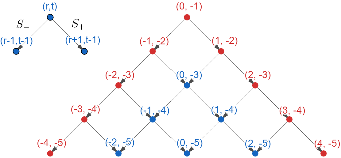
Figure 1. Path-connected components of the space of Legendrian unknots. The red dots indicate that the hypothesis of Theorem 1.2.1 are fullfilled.

Remark 1.2.2.

This result says that any multiparametric family of smooth long unknots can be homotoped into a family of long Legendrian unknots. However, it is important to note that this homotopy is not $C^{0}$-close. It is not possible to find a $\operatorname{tb}=-1$ Legendrian unknot arbitrarily close to a stabilized Legendrian unknot [RS22].

The path-connected components of the space of oriented Legendrian unknots in a tight contact $3$-manifold are understood due to Eliashberg-Fraser Theorem [EF09]. Every Legendrian unknot is obtained from the unique Legendrian unknot with $\operatorname{tb}=-1$ by a finite sequence of positive and negative stabilizations. See Figure 1.

We will also prove the same statement for transverse unknots with self-linking number $-1$ in tight contact $3$-manifolds (Theorem 4.3.1). It should be mentioned that this result is purely $3$-dimensional as the work in preparation of Eliashberg and Kragh shows [EK]: in the higher dimensional standard $({\mathbb{R}}^{2n+1},\xi_{\operatorname{std}})$ there are exotic families of long Legendrian unknots. Here, exotic refers to formally contractible but not geometrically contractible, see [Mur12, FMAP20]. The analog question in the transverse case is about the topology of the space of codimension $2$ contact spheres which has recently received attention [CPP21, HH19]. The work of Honda-Huang [HH19] and Eliashberg-Pancholi [EP22] about higher dimensional convexity could bring some light in this direction.

We particularize the previous result to the case of $({\mathbb{S}}^{3},\xi_{\operatorname{std}})$. Denote by ${\mathfrak{Trans}}^{0}({\mathbb{S}}^{3},\xi_{\operatorname{std}})$ the space of parametrized positively transverse unknots with self-linking number $-1$. We will call Legendrian great circle to the unknot obtained as the intersection of a Lagrangian plane in ${\mathbb{C}}^{2}$ with ${\mathbb{S}}^{3}$ and transverse great circle to the intersection of a complex plane in ${\mathbb{C}}^{2}$ with ${\mathbb{S}}^{3}$.

Theorem 1.2.3 (Theorem 3.3.6 and Corollary 4.3.2).

• The space ${\mathfrak{Leg}}^{(-1,0)}({\mathbb{S}}^{3},\xi_{\operatorname{std}})$ is homotopy equivalent to $\operatorname{U}(2)$, the space of parametrized Legeandrian great circles.

• The space ${\mathfrak{Trans}}^{0}({\mathbb{S}}^{3},\xi_{\operatorname{std}})$ is homotopy equivalent to $\operatorname{SU}(2)$, the space of parametrized transverse great circles.

This is the Contact version of the Theorem of Hatcher that states the smooth analog of this result. Namely, that the space of parametrized smooth unknots in ${\mathbb{S}}^{3}$ is homotopy equivalent to $V_{4,2}=\operatorname{SO}(4)/\operatorname{SO}(2)$, the space of parametrized great circles [Hat83, Hat99b]. This answers positively a question posed in [CDRGG15, Remark 4.2]. To deduce this result we will use the knowledge of the homotopy type of the space smooth long unknots [Hat83]. See also Budney [Bud10].

1.2.2. Legendrian $(n,n)$-torus links with max-$\operatorname{tb}$.

We also determine the homotopy type of the space $\mathcal{L}_{n}$ of embeddings of the max-$\operatorname{tb}$ $(n,n)$-torus link into $({\mathbb{S}}^{3},\xi_{\operatorname{std}})$:

Theorem 1.2.4.

Let $\mathcal{M}_{n}$ be the mapping class group of a $2$-sphere with $n$-holes. There is a homotopy equivalence $\mathcal{L}_{n}\cong\operatorname{U}(2)\times K(\mathcal{M}_{n},1)$.

This result should be compared with the work of Casals and Gao [CG22] about the $(4,4)$-torus link. In that article the authors use invariants from microlocal sheaf theory to build a surjection of the fundamental group of the space of unparametrized $(4,4)$-torus links over the mapping class group of the $2$-sphere with $4$ marked points.

1.3. Outline

The article is organized as follows. In Section 2 we present background material. In Section 3 we study the homotopy type of certain spaces of convex embeddings. In particular, in Subsection 3.2 we prove Theorems 1.0.1 and 1.0.2. In Subsection 3.3 the proof of our results about universally tight handlebodies are provided and also the result relating the homotopy type of the contactomorphism group with the topology of the space of Giroux skeletons. In Section 4 we prove Theorem 1.2.1. Finally, in Section 5 we provide the proofs of Theorems 1.1.3, 1.1.4 and 1.2.4. We also prove a result about the existence of common trivializations for multi-parametric families of tight ${\mathbb{R}}^{3}$.

Notation. Let $(M,\xi)$ be a compact contact manifold with possibly non-empty boundary. We will denote by ${\mathfrak{C}Str}(M)$ the space of contact structures on $M$ that coincide with $\xi$ near $\partial M$ and by ${\mathfrak{C}Str}(M,\xi)$ the path–connected component containing $\xi$. The group of orientation preserving diffeomorphisms of $M$ that are the identity near the boundary will be denoted by $\operatorname{Diff}(M)$ and the subgroup of diffeomorphisms isotopic to the identity by $\operatorname{Diff}_{0}(M)$. We will denote by $\operatorname{Cont}(M,\xi)\subseteq\operatorname{Diff}(M)$ the subgroup of contactomorphisms of $(M,\xi)$ while $\operatorname{Cont}_{0}(M,\xi)=\operatorname{Diff}_{0}(M)\cap\operatorname{Cont}(M,\xi)$ will stand for the subgroup of contactomorphisms smoothly isotopic to the identity. The space of Legendrian embeddings of ${\mathbb{S}}^{1}$ into $(M,\xi)$ will be denoted by ${\mathfrak{Leg}}(M,\xi)$. For a given subset $C\subseteq M$ we will denote by ${\mathcal{O}p}(C)$ an arbitrarily small and unspecified open neighbourhood of $C$. The notation $\operatorname{rel}C$ will always mean relative to ${\mathcal{O}p}(C)$, for instance, for a point $p\in M$ the notation $\operatorname{Diff}(M;\operatorname{rel}p)\subseteq\operatorname{Diff}(M)$ stands for those diffeomorphisms that are the identity over ${\mathcal{O}p}(p)$. Finally, ${\mathfrak{Emb}}(S,M)$ will denote the space of embeddings of $S$ into $M$ that coincide over ${\mathcal{O}p}(\partial S)$ with a prefixed embedding (that will be clearly specified). If we drop the condition of being fixed near the boundary we will explicitly state it. All these spaces are equipped with the $C^{\infty}$ topology.

Acknowledgements. Special thanks to Ángel González for the uncountable number of hours that he has spent listening to us. We are grateful to V. Colin for valuable conversations. We want to acknowledge the interest and kindness of Ryan Budney that explained to us very basic things when we were getting into the fascinating world of smooth embeddings theory. Moreover, he was a great host when we visited him in Victoria where he taught us about sophisticated homotopy computations and what is more important about crab fishing and digesting. First author wants to thank Roger Casals, Yasha Eliashberg and Viktor Ginzburg for hosting him and asking him all the right questions in a visit to California in which this whole project unexpectedly began to take shape. Part of this project was developed while he was visiting the Institute for Advanced Studies in 2021, he would like to acknowledge the hospitality of the centre. He is also grateful to Fabio Gironella, Gordana Mátic, Hyunki Min, Juan Muñoz-Echániz and Dishant Pancholi for valuable discussions. Finally, he really appreciates the encouragement provided by Y. Eliashberg, D. Pancholi, G. Sánchez and, his wonderful advisor, F. Presas; after realizing that a previous preprint version of this article was wrong. The second author wants to thank Álvaro del Pino for his support and interest in this project. Also he would like to thank the Geometry group at Utrecht University where he was given a nice environment to develop this and other projects. The authors want to acknowledge the support of the Spanish national grant with reference number PID2019-108936GB-C21 (MINECO/FEDER) and by the excellence project CEX2019-000904-S. The first author was supported by Beca de Personal Investigador en Formación UCM. During the development of this work, the second author has been funded by Programa Predoctoral de Formación de Personal Investigador No Doctor del Departamento de Educación del Gobierno Vasco.

2. Preliminaries.

This Section reviews several quite standard results in Contact Topology. Though, they are very standard for the expert in each subarea, it may happen that even the usual reader of Contact Topology is not familiar with some of them. As for the last two Subsections, they are focused in a number of standard results of $3$-dimensional differential topology. Specially remarkable for us is Lemma 2.6.2 that is used in a continuous way all over the article. It is a frequent tool in algebraic topology and probably less frequent in contact topology.

2.1. Convex surface theory in contact $3$–manifolds.

We will recall some facts about Convex Surface Theory that we will need in the article. The reader is referred to [Etn04, Hon00a, HH19, Gir91, Mas14] for further details.

Let $(M,\xi)$ be a contact $3$-manifold. A properly embedded surface $S\subseteq M$ is said to be convex if there exists a contact vector field $X$ that is transverse to $S$. A convex embedding of $S$ into $(M,\xi)$ is any embedding $e:S\rightarrow M$ such that $e(S)\subseteq M$ is convex. We will fix an orientation on $\Sigma$ and also require the embeddings to respect this orientation. The $1$–dimensional singular foliation $e^{*}\xi$ on $S$ is called the characteristic foliation of the surface. A convex surface $S$ has a neighbourhood in $M$ contactomorphic to $(S\times{\mathbb{R}},\ker(fdt+\beta))$ where $t$ is the ${\mathbb{R}}$–coordinate, $\beta\in\Omega^{1}(S)$ is the pullback, via the inclusion, of some contact form $\alpha$ of $(M,\xi)$ to $S$, and $f\in C^{\infty}(S)$. The zero set of $f$ defines an embedded $1$–dimensional submanifold of $\Gamma\subseteq S$ that is called the dividing set. This construction depends on the choice of the contact vector field $X$, but since the space of contact vector fields transverse to $S$ is contractible the isotopy class of $\Gamma$ is well–defined. We will write $\Gamma_{X}$ instead of $\Gamma$ whenever we want to make clear the choice of contact vector field that we are using. Do note that $\Sigma\setminus\Gamma_{X}=\Sigma_{+}\sqcup\Sigma_{-}$, where $\Sigma_{+}\subseteq\Sigma$ is the subsurface of $\Sigma\setminus\Gamma_{X}$ in which the orientation of the line field generated by $X$, determined by the orientation of $\Sigma$ and the orientation of $M$; and the coorientation of $\xi$ coincide; and $\Sigma_{-}$ in which they are opposite.

Theorem 2.1.1 (Giroux Approximation Theorem [Gir01b, Hon00a]).

Let $(M,\xi)$ be any contact $3$–manifold. Let $S\subseteq M$ be a compact surface. If $S$ has non-empty boundary we assume that is Legendrian and that the twisting number between the contact framing of the normal framing of $\partial S$ and the induced by $S$ is negative. Then,

• If $\partial S=\emptyset$ there exists a $C^{\infty}$ perturbation of $S$ that makes it convex.

• If $\partial S\neq\emptyset$ there exists a pertubation, fixed at the boundary, which is $C^{0}$ near the boundary and $C^{\infty}$ in the interior, of $S$ that makes it convex.

We will apply the previous Theorem to families of disks which share a small neighborhood of the boundary, so we will be assuming that they will be convex near the boundary. This allows us to assume that the perturbation is $C^{\infty}$ small in those applications.

Theorem 2.1.2 (Giroux Tightness Criterion [Gir01a]).

Let $S\subseteq(M,\xi)$ be a convex surface in a tight contact $3$–manifold. Then,

• if $S$ is a sphere the dividing set is connected,

• if $S$ is not a sphere the dividing set does not contain any homotopically trivial curve.

Let $e:S\rightarrow(M,\xi)$ be a convex embedding. Denote the characteristic foliation of $S$ by $\mathcal{F}=e^{*}\xi$. Denote by ${\mathfrak{Emb}}(S,(M,\xi),\mathcal{F})$ the space of embeddings $j:S\rightarrow M$ such that $j^{*}\xi=\mathcal{F}$. Fix a contact vector field $X$ transverse to $e(S)$ and let $\Gamma_{X}$ be the dividing set defined by $X$. Denote by ${\mathfrak{Emb}}(S,(M,\xi),\Gamma_{X})$ the space of embeddings $j:S\rightarrow M$ such that $j^{*}\xi$ is divided by $\Gamma_{X}$. In the case that $\partial S\neq\emptyset$ we assume that all the embeddings coincide in an open neighbourhood of the boundary and that the boundary is Legendrian.

Theorem 2.1.3 (Giroux Realization Theorem [Gir01b]).

The natural inclusion

$${\mathfrak{Emb}}(S,(M,\xi),\mathcal{F})\hookrightarrow{\mathfrak{Emb}}(S,(M,\xi),\Gamma_{X})$$

is a homotopy equivalence.

The deformations in the previous result are realized by admissible isotopies; i.e. graphical deformations of $S\subseteq S\times{\mathbb{R}}$ where the ${\mathbb{R}}$-factor is determined by the contact vector field $X$. It is useful to have a practical criterion to determine which curves and arcs in a surface can be realized as part of the characteristic foliation of a convex surface. Let $S\subset(M,\xi)$ be a convex surface with Legendrian boundary and dividing set $\Gamma$. A collection of disjoint and properly embedded curves and arcs $C\subseteq S$ is said to be non-isolating if: $C$ is transverse to $\Gamma$, every arc in $C$ starts and ends at $\Gamma$ and every component of $S\backslash(C\cup\Gamma)$ has a boundary component that intersects $\Gamma$. The following result, due to K. Honda, provides this criterion

Theorem 2.1.4 (Legendrian Realization Principle, Theorem 3.7 in [Hon00a]).

Let $S\subseteq(M,\xi)$ be a convex surface with Legendrian boundary and dividing set $\Gamma$. If a collection of disjoint properly embedded curves and arcs $C\subseteq S$ is non-isolating then there exists a singular foliation $\mathcal{F}$ of $S$ divided by $\Gamma$ and such that $C\subseteq\mathcal{S}$.

In other words, there exists an admissible isotopy of convex surfaces in such a way that $C$ becomes Legendrian (Theorem 2.1.3) We will also use the following technical lemma that appear in [Hon00a]. See also [Yut97].

Lemma 2.1.5.

[Hon00a, Yut97] Let $\Sigma,\Sigma^{\prime}\subseteq(M,\xi)$ be two embedded convex surfaces with dividing sets $\Gamma\subseteq\Sigma$ and $\Gamma^{\prime}\subseteq\Sigma^{\prime}$. Assume that $\partial\Sigma^{\prime}\subseteq\Sigma$ is Legendrian. Then between two adjancent points of $\Gamma\cap\partial\Sigma$ there is a point of $\Gamma^{\prime}\cap\partial\Sigma^{\prime}$ and vice versa.

The following technical proposition, due to E. Giroux, will be really useful.

Proposition 2.1.6.

[Gir01b, GM17] Let $(M,\xi)$ be any compact contact $3$-manifold with convex boundary. Denote by $\Gamma\subseteq\partial M$ the dividing set and by ${\mathfrak{C}Str}(M;\Gamma)$ the space of contact structures on $M$ with convex boundary and dividing set $\Gamma$. Then, the homotopy type of $\operatorname{Cont}(M,\hat{\xi})$, $\hat{\xi}\in{\mathfrak{C}Str}(M;\Gamma)$, only depends on the connected component of ${\mathfrak{C}Str}(M;\Gamma)$ containing $\hat{\xi}$.

We will also use extensively the relation between the configuration of the dividing set of a convex Seifert surface for a Legendrian $L$ and the formal invariants of $L$, observered by Y. Kanda [Kan98]. Since we will only use it for Legendrian unknots and Seifert disks in tight contact $3$-folds we will state it just in this case.

Lemma 2.1.7.

(Theorem 2.30 in [Etn04]) Let $L\subseteq(M,\xi)$ be any Legendrian unknot in tight contact $3$-manifold. Let ${\mathbb{D}}^{2}$ be any convex Seifert disk for $L$ with dividing set $\Gamma$. Denote by $\#\Gamma$ the number of connected components of the dividing set and by $\#CC(+)$ (resp. $\#CC(-)$) the number of connected components of the positive (resp. negative) region of ${\mathbb{D}}^{2}$. Then, the formal invariants of the oriented Legendrian knot $L$ satisfy the following equalities

• $\operatorname{tb}(L)=-\#\Gamma$ and

• $\operatorname{rot}(L)=\#CC(+)-\#CC(-).$

2.2. Fibrations in contact topology.

The following lemma is well known. A good source for most of the fibrations that we are going to describe are the P. Massot notes [Mas15] which are a detailed version of the results explained in [GM17]. The reader is also referred to [Gei08] where the non-parametric version of these results are also proven.

Let $(M,\xi)$ be a contact $3$-manifold. Fix a Legendrian $\gamma\in{\mathfrak{Leg}}(M,\xi)$. Consider also an embedding $e:S\rightarrow M$ of a compact surface into $M$, with characteristic foliation $\mathcal{F}=e^{*}\xi$, and the space ${\mathfrak{Emb}}(S,(M,\xi);\mathcal{F})$ the space of embeddings $j:S\rightarrow M$ such that $j^{*}\xi=\mathcal{F}$ and coincide with $e$ near $\partial S$.

Lemma 2.2.1.

• The map $\operatorname{Cont}(M,\xi)\rightarrow{\mathfrak{Leg}}(M,\xi),\varphi\mapsto\varphi\circ\gamma;$ is a fibration with fiber $\operatorname{Cont}(M,\xi;\operatorname{rel}\gamma({\mathbb{S}}^{1}))$.

• The map $\operatorname{Diff}_{0}(M)\rightarrow{\mathfrak{C}Str}(M,\xi),\varphi\mapsto\varphi_{*}\xi;$ is a fibration with fiber $\operatorname{Cont}_{0}(M,\xi).$

• The map $\operatorname{Cont}(M,\xi;\operatorname{rel}e(\partial S))\rightarrow{\mathfrak{Emb}}(S,(M,\xi);\mathcal{F}),\varphi\mapsto\varphi\circ e;$ is a fibration with fiber $\operatorname{Cont}(M,\xi;\operatorname{rel}e(S))$.

2.3. The space of Darboux balls in a contact manifold.

Alexander’s trick allows to prove that the space ${\mathfrak{Emb}}^{+}({\mathbb{D}}^{n},{\mathbb{R}}^{n})$ of orientation preserving embeddings ${\mathbb{D}}^{n}\rightarrow{\mathbb{R}}^{n}$ linearise, i.e. it is homotopy equivalent to $\operatorname{GL}^{+}(n,{\mathbb{R}})$. This, together with the Isotopy Extension Theorem, implies that on a closed oriented $n$–manifold $N^{n}$ the space ${\mathfrak{Emb}}^{+}({\mathbb{D}}^{n},N^{n})$ is homotopy equivalente to the total space of the oriented frame bundle $\operatorname{Fr}^{+}(N)$. Explicitly, there is a map of fibrations

Where the maps between the fibers and the bases are homotopy equivalences. Thus, the natural map ${\mathfrak{Emb}}^{+}({\mathbb{D}}^{n},N^{n})\rightarrow\operatorname{Fr}^{+}(N^{n})$ is a homotopy equivalence.

In the contact category there is also an Alexander trick. Indeed, in $({\mathbb{R}}^{2n+1},\xi_{\operatorname{std}}=\ker(dz-\sum_{i}y_{i}dx_{i}))$ the dilation

$$\delta_{t}:{\mathbb{R}}^{2n+1}\rightarrow{\mathbb{R}}^{2n+1},(\textbf{x},\textbf{y},z)\mapsto(t\textbf{x},t\textbf{y},t^{2}z);$$

is a contactomorphism for every $t>0$. Thus, the space ${\mathfrak{CEmb}}(({\mathbb{D}}^{2n+1},\xi_{\operatorname{std}}),({\mathbb{R}}^{2n+1},\xi_{\operatorname{std}}))$ of co–oriented embeddings of Darboux balls into $({\mathbb{R}}^{2n+1},\xi_{\operatorname{std}})$ is homotopy equivalent to the space of contact framings, i.e. to $\operatorname{U}(n)$. We refer the reader to [Gei08, Section 2.6.2] for further details. In particular, the Isotopy Extension Theorems in Contact Topology implies, in the same way as in the smooth case, that

Lemma 2.3.1.

Let $(N,\xi)$ be a closed co–oriented $(2n+1)$–contact manifold. The space ${\mathfrak{CEmb}}(({\mathbb{D}}^{2n+1},\xi_{\operatorname{std}}),(N,\xi))$ is homotopy equivalent to the total space of the bundle of contact framings $\operatorname{CFr}(N,\xi)$ over $(N,\xi)$, which has fiber $\operatorname{U}(n)$; i.e. a Darboux ball is determined by the centre of the ball and the induced framing of $\xi$ at that point.

2.4. Legendrian embeddings in $({\mathbb{S}}^{3},\xi_{\operatorname{std}})$.

Let $({\mathbb{S}}^{3},\xi_{\operatorname{std}})$ be the standard tight contact $3$–sphere, i.e. $\xi_{\operatorname{std}}$ is defined as the complex tangencies of $T{\mathbb{S}}^{3}$ with respect to the standard complex structure in ${\mathbb{C}}^{2}\supseteq{\mathbb{S}}^{3}$.

Let ${\mathfrak{Leg}}_{N,jN}({\mathbb{S}}^{3},\xi_{\operatorname{std}})=\{\gamma\in{\mathfrak{Leg}}({\mathbb{S}}^{3},\xi_{\operatorname{std}}):\gamma(0)=N,\gamma^{\prime}(0)=jN\}$ be the space of long Legendrian embeddings. This space is homotopy equivalent with the space of long Legendrian embeddings in the usual knot theorist sense: Legendrian embeddings into $({\mathbb{S}}^{3},\xi_{\operatorname{std}})$ that coincide in an open neighbourhood of the north pole $N$ with the Legendrian great circle $\gamma(t)=(\cos t,\sin t)\in{\mathbb{S}}^{3}\subseteq{\mathbb{C}}^{2}$. This justifies the name of the space.

Lemma 2.4.1.

There exists a homotopy equivalence

(5) $$\Phi:{\mathfrak{Leg}}({\mathbb{S}}^{3},\xi_{\operatorname{std}})\rightarrow\operatorname{U}(2)\times{\mathfrak{Leg}}_{N,jN}({\mathbb{S}}^{3},\xi_{\operatorname{std}}).$$

Proof.

We assume without loss of generality that all the Legendrian embeddings $\gamma$ satisfy that $||\gamma^{\prime}(0)||=1$. By the Legendrian condition we have a natural map ${\mathfrak{Leg}}({\mathbb{S}}^{3},\xi_{\operatorname{std}})\rightarrow\operatorname{U}(2),\gamma\mapsto A_{\gamma}=(\gamma(0)|\gamma^{\prime}(0)).$ The homotopy equivalence is given by

(6) $$\begin{array}[]{rccl}\Phi:{\mathfrak{Leg}}({\mathbb{S}}^{3},\xi_{\operatorname{std}})&\longrightarrow&\operatorname{U}(2)\times{\mathfrak{Leg}}_{N,jN}({\mathbb{S}}^{3},\xi_{\operatorname{std}})\\ \gamma&\mapsto&(A_{\gamma},A_{\gamma}^{-1}\gamma).\end{array}$$

∎

2.5. Smooth Case. Hatcher’s Theorems.

In this Section we recall some known results of A. Hatcher that we will use later in the article.

2.5.1. The Smale Conjecture.

The main ingredient to understand the topology of the diffeomorphism group of a $3$-fold is the proof given by A. Hatcher of the Smale Conjecture

Theorem 2.5.1 ([Hat83]).

The group of diffeomorphisms $\operatorname{Diff}({\mathbb{D}}^{3})$ of the $3$–ball fixing the boundary pointwisely is contractible.

2.5.2. Embeddings of disks into irreducible $3$-manifolds.

Let $M^{3}$ be a orientable compact connected irreducible $3$–manifold with boundary. Let $i:{\mathbb{D}}^{2}\hookrightarrow M^{3}$ be a proper embedding of the $2$–disk into $M$ and consider the space ${\mathfrak{Emb}}({\mathbb{D}}^{2},M^{3})$ of embeddings $\phi:{\mathbb{D}}^{2}\rightarrow M^{3}$ such that $\phi_{|{\mathcal{O}p}(\partial{\mathbb{D}}^{2})}=i_{|{\mathcal{O}p}(\partial{\mathbb{D}}^{2})}$. The following holds

Theorem 2.5.2 (Hatcher [Hat99a]).

The space ${\mathfrak{Emb}}({\mathbb{D}}^{2},M^{3})$ is contractible.

Corollary 2.5.3.

Let $H^{g}$ be the genus $g$ handlebody. The diffeomorphism group $\operatorname{Diff}(H^{g})$ is contractible.

Proof.

Since $\operatorname{Diff}({\mathbb{D}}^{3})$ is contractible because of Theorem 2.5.1, it is enough to check that $\operatorname{Diff}(H^{g})$ is homotopy equivalent to $\operatorname{Diff}(H^{g-1})$ for any $g\geq 1$. Consider any proper embedding of a separating disk $e:{\mathbb{D}}^{2}\rightarrow H^{g}$. The postcomposition of $e$ by any diffeomorphism of $H^{g}$ induces a fibration

$$\operatorname{Diff}(H^{g}\backslash e({\mathbb{D}}^{2}))\rightarrow\operatorname{Diff}(H^{g})\rightarrow{\mathfrak{Emb}}({\mathbb{D}}^{2},H^{g}).$$

The fiber can be identified with $\operatorname{Diff}(H^{g-1})$ and the base is contractible by Theorem 2.5.2 so the result follows. ∎

An important consequence of the previous result is the following

Theorem 2.5.4 (Hatcher).

The path–connected component ${\mathfrak{Emb}}^{0}_{N,jN}({\mathbb{S}}^{1},{\mathbb{S}}^{3})$ of the space of smooth long embeddings containing the unknot is contractible.

Proof.

In view of the fibration (2) it is enough to check that the space $\operatorname{Diff}({\mathbb{D}}^{2}\times{\mathbb{S}}^{1})$ is contractible. This follows from Corollary 2.5.3. ∎

In general, it follows that each path-connected component of the space of long embeddings in ${\mathbb{S}}^{3}$ is a $K(\pi,1)$ space [Hat83].

2.6. Microfibration Lemma

We will make use of the following notion introduced by M.Gromov in [Gro86].

Definition 2.6.1.

A map $p:E\rightarrow B$ is a Serre microfibration if for any $k\geq 0$ and any pair of maps $h:{\mathbb{D}}^{k}\times[0,1]\rightarrow B$ and $g:{\mathbb{D}}^{k}\times\{0\}\rightarrow E$ such that $p\circ g=h_{|{\mathbb{D}}^{k}\times\{0\}}$ there exists a positive number $\varepsilon>0$ and a map $\hat{g}:{\mathbb{D}}^{k}\times[0,\varepsilon]\rightarrow E$ satisfying that

• $\hat{g}_{|{\mathbb{D}}^{k}\times\{0\}}=g$ and

• $p\circ\hat{g}=h_{{\mathbb{D}}^{k}\times[0,\varepsilon]}$.

The following result was also hinted by M. Gromov in [Gro86]

Lemma 2.6.2 (Microfibration Lemma [Wei05]).

Let $p:E\rightarrow B$ be a Serre microfibration with weakly contractible non-empty fibers. Then $p$ is a Serre fibration.

3. Eliashberg-Mishachev and Giroux Theorems.

We need the parametric versions of two Theorems due to Eliashberg-Mishachev for tight contact structures in ${\mathbb{S}}^{3}$ or in ${\mathbb{D}}^{3}$ and one due to Giroux. We claim that the first two are already proven: contractibility of the space of contact structures in the ball and contractibility of the space of contactomorphisms [EM21]. In fact, they are completely equivalent using Theorem 2.5.1. However, the third and the fourth statements require a proof. The third one is the heart of the article: a multiparametric convex surface theory. In fact, we cheat a bit. We use the contractibility of the space of contactomorphisms of the ball to prove right away that the space of convex disks with fixed characteristic foliation in the ball is also contractible. A matter of algebraic topology force game: diffeomorphisms are contractible in the ball, contactomorphisms are contractible in the ball, then standard convex disks are contractible in the ball. It comes in two flavours the already mentioned one and another one for multiparametric families of standard spheres, where a homotopy equivalence is not obtained, since some formal evaluation data needs to be fixed.

3.1. Contact topology of the standard $3$-disk.

3.1.1. Classification of tight contact structures in the $3$–sphere.

We have the following Theorem, due to Eliashberg that completely characterizes the connectedness of the subspace of tight contact structures homotopic to the standard one in ${\mathbb{S}}^{3}$.

Theorem 3.1.1 (Theorem 2.1.1 in [Eli92]).

A tight contact structure on ${\mathbb{S}}^{3}$ is isotopic to the standard contact structure $\xi_{{\operatorname{std}}}$

In fact, this result holds in a multi parametric fashion. This version was stated without a proof in [Eli92], a full proof due to Eliashberg and Mishachev appeared recently in [EM21]. There is also an approach to prove this result following techniques of convex surface theory in the thesis of D. Jänichen [Jä18]. Let ${\mathfrak{C}Str}({\mathbb{S}}^{3},\xi_{\operatorname{std}})$ be the space of tight contact structures on ${\mathbb{S}}^{3}$. Identify the space of isometric linear complex structures on ${\mathbb{C}}^{2}$ that induce the right orientation with the $2$-sphere

$${\mathbb{S}}^{2}={\mathbb{S}}^{2}(i,j,k)=\{J_{p_{1},p_{2},p_{3}}=p_{1}i+p_{2}j+p_{3}k:(p_{1},p_{2},p_{3})\in{\mathbb{S}}^{2}\}.$$

Then, we have an inclusion

(7) $$i:{\mathbb{S}}^{2}(i,j,k)\rightarrow{\mathfrak{C}Str}({\mathbb{S}}^{3},\xi_{\operatorname{std}}),J\mapsto\xi_{J}=T{\mathbb{S}}^{3}\cap JT{\mathbb{S}}^{3}.$$

This inclusion is, in fact, a homotopy injection since the evaluation map

$$\operatorname{ev}_{N}:{\mathfrak{C}Str}({\mathbb{S}}^{3},\xi_{\operatorname{std}})\to\operatorname{SO}(4)/\operatorname{U}(2)={\mathbb{S}}^{2}$$

of the contact structure at the north pole on $N\in{\mathbb{S}}^{3}$, defines a left inverse for it. Even more,

Theorem 3.1.2 ([EM21]).

The map $\operatorname{ev}_{N}$ is a homotopy equivalence.

3.1.2. Contactomorphisms in the standard contact $3$–sphere.

Consider the natural inclusion

(8) $$i:\operatorname{U}(2)\hookrightarrow\operatorname{Cont}({\mathbb{S}}^{3},\xi_{{\operatorname{std}}}).$$

Observe that this map defines a homotopy injection. Indeed, this follows by observing that

(9) $$\operatorname{ev}_{N}:\operatorname{Cont}({\mathbb{S}}^{3},\xi_{{\operatorname{std}}})\to\operatorname{U}(2),$$

defined by evaluating the image of the north pole and the jacobian at the north pole, defines a left inverse for $i$.

Corollary 3.1.3.

The evaluation map (9) is a homotopy equivalence.

Proof.

Consider the diagram,

The result follows from Theorems 2.5.1 and 3.1.2 ∎

Corollary 3.1.4.

The space of compactly supported contactomorphisms of the $3$–ball for the standard contact structure $\operatorname{Cont}({\mathbb{D}}^{3},\xi_{\operatorname{std}})$ is contractible.

This is an obvious consequence of $\operatorname{Cont}({\mathbb{D}}^{3},\xi_{\operatorname{std}})$ being the fiber of the map (9). As a consequence of this result and the Theorems of Giroux explained in 2.1 one concludes that the same statement holds for any tight contact structure on the $3$–ball:

Corollary 3.1.5.

Let $\xi_{\operatorname{Tight}}$ be any tight contact structure on ${\mathbb{D}}^{3}$. The group $\operatorname{Cont}({\mathbb{D}}^{3},\xi_{\operatorname{Tight}})$ of compactly supported contactomorphisms of $({\mathbb{D}}^{3},\xi_{\operatorname{Tight}})$ is contractible.

Proof.

Let $\varphi^{z}\in\operatorname{Cont}({\mathbb{D}}^{3};\xi_{\operatorname{Tight}})$ be any family of contactomorphisms. Let ${\mathbb{S}}^{2}\times[0,1]\hookrightarrow{\mathbb{D}}^{3}$ be a collar neighbourhood of $\partial{\mathbb{D}}^{3}={\mathbb{S}}^{2}={\mathbb{S}}^{2}\times\{0\}$ such that $\varphi^{z}_{|{\mathbb{S}}^{2}\times[0,1]}$ is the identity. By Giroux Genericity Theorem we may assumme that ${\mathbb{S}}^{2}\times\{\frac{1}{2}\}$ is convex. Moreover, the dividing set can be assumed to be the equator of the sphere by Giroux Tightness Criterion. Finally, by Giroux Realizability the characteristic foliation can be assumed to be standard, meaning by this that the characteristic foliation of ${\mathbb{S}}^{2}\times\{\frac{1}{2}\}$ induced by $\xi_{\operatorname{Tight}}$ coincides with the characteristic foliation induced by the standard tight contact structure $\xi_{\operatorname{std}}$ on the boundary of the disk ${\mathbb{S}}^{2}=\partial{\mathbb{D}}^{3}$. Thus, since there is only one tight contact structure, up to isotopy relative to the boundary, on ${\mathbb{D}}^{3}$ such that the characteristic foliation at the boundary coincides with the induced by $\xi_{\operatorname{std}}$; the initial family $\varphi^{z}\in\operatorname{Cont}({\mathbb{D}}^{3},\xi_{\operatorname{Tight}})$ can be regarded as a family of contactomorphisms of the standard tight $3$-ball $({\mathbb{D}}^{3},\xi_{\operatorname{std}})$. In particular it is contractible because of the previous result. ∎

3.2. The Microfibration Trick.

In this Subsection we introduce the Microfibration Trick which is some sort of variation of Colin’s Discretization Technique [Col97] which applies parametrically. We will use this idea to prove several results concerning the topology of the space of convex embeddings of disks with Legendrian boundary and convex spheres into a tight contact $3$-manifold. In the first case we will impose some conditions on the formal invariants of the Legendrian unknot bounded by the disks. In general, this method can be applied if the following two conditions are satisfied:

• The space of convex embeddings $S\hookrightarrow(M,\xi)$ with fixed characteristic foliation $\mathcal{F}$ is dense into the space of smooth embeddings.

• We understand, at a homotopy level, the inclusion of the space of convex embeddings $S\hookrightarrow(S\times{\mathbb{R}},\xi)$, with fixed characteristic foliation $\mathcal{F}$, of $S$ into a vertically invariant neighbourhood, into the space of smooth embeddings.

Do note that Colin’s trick requires the exactly same hypothesis at a $\pi_{0}$-level. The first condition is really restrictive so we will be able to prove statements in general tight $3$-manifolds just for simple cases.

3.2.1. The space of standard disks in a tight $3$-fold.

Denote by $({\mathbb{D}}^{2},\mathcal{F}_{\operatorname{std}})$ the standard foliation of the disk with boundary the Legendrian unknot with $\operatorname{tb}=-1$. That is, the characteristic foliation has two elliptic points of opposite signs at the boundary and Legendrian leaves joining them. See Figure 2. We will say that an embedding $e:{\mathbb{D}}^{2}\rightarrow(M^{3},\xi)$ of a disk into a contact $3$–fold is standard if it is convex and $({\mathbb{D}}^{2},e^{*}\xi)=({\mathbb{D}}^{2},\mathcal{F}_{\operatorname{std}})$. In particular, the boundary of $e({\mathbb{D}}^{2})$ is a standard Legendrian unknot, that is, with $\operatorname{tb}=-1$.

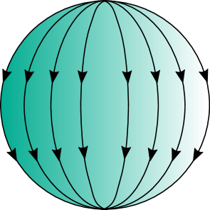
Figure 2. The standard convex disk.

Let $e:{\mathbb{D}}^{2}\rightarrow(M,\xi)$ be an standard embedding of a disk into a contact $3$–fold. Denote by ${\mathfrak{Emb}}({\mathbb{D}}^{2},M)$ the space of smooth embeddings $f:{\mathbb{D}}^{2}\rightarrow M$ such that $f_{|{\mathcal{O}p}(\partial{\mathbb{D}}^{2})}=e_{|{\mathcal{O}p}(\partial{\mathbb{D}}^{2})}$. Similarly, define ${\mathfrak{Emb}}_{\operatorname{std}}({\mathbb{D}}^{2},(M,\xi))$ as the subspace of ${\mathfrak{Emb}}({\mathbb{D}}^{2},M)$ conformed by embeddings that are standard.

We will use the following technical definition

Definition 3.2.1.

Let $N$ be a compact manifold and $(M,g)$ a Riemannian manifold. Denote by ${\mathfrak{Emb}}_{\mathcal{P}}(N,M)\subseteq{\mathfrak{Emb}}(N,M)$ the subspace of embeddings that satisfies certain property $\mathcal{P}$. We will say that the inclusion

$$j:{\mathfrak{Emb}}_{\mathcal{P}}(N,M)\hookrightarrow{\mathfrak{Emb}}(N,M)$$

is a $C^{0}$-dense homotopy equivalence if

• $j$ is a homotopy equivalence.

• For any $\varepsilon>0$ and any continuous map $\varphi:K\rightarrow{\mathfrak{Emb}}(N,M)$ from a compact parameter space $K$ there exists an homotopy $\varphi_{t}:K\rightarrow{\mathfrak{Emb}}(N,M)$, $t\in[0,1]$, such that

  1. $\varphi_{0}=\varphi$,

  2. ${\operatorname{Image}}(\varphi_{1})\subseteq{\mathfrak{Emb}}_{\mathcal{P}}(N,M)$ and

  3. $\varphi_{t}(k)(N)\subseteq{\mathbb{B}}(N,\varepsilon)=\{p\in M:d_{M}(p,N)<\varepsilon\}$.

Our main result can be stated as follows.

Theorem 3.2.2.

Let $(M,\xi)$ be a tight contact $3$-manifold. The inclusion

$${\mathfrak{Emb}}_{\operatorname{std}}({\mathbb{D}}^{2},(M,\xi))\hookrightarrow{\mathfrak{Emb}}({\mathbb{D}}^{2},M)$$

is a $C^{0}$-dense homotopy equivalence.

First let us prove Theorem 3.2.2 in the case of a tight $3$-ball.

Lemma 3.2.3.

Let $({\mathbb{D}}^{3},\xi_{\operatorname{Tight}})$ be any tight contact structure on the $3$–ball. Fix coordinates $(x,y,z)\in{\mathbb{D}}^{3}$ and assumme that $e:{\mathbb{D}}^{2}(x,y)\hookrightarrow({\mathbb{D}}^{3},\xi_{\operatorname{Tight}}),(x,y)\mapsto(x,y,0)$ is an standard embedding. Then, the inclusion

$${\mathfrak{Emb}}_{\operatorname{std}}({\mathbb{D}}^{2},({\mathbb{D}}^{3},\xi_{\operatorname{Tight}}))\hookrightarrow{\mathfrak{Emb}}({\mathbb{D}}^{2},{\mathbb{D}}^{3})$$

is a homotopy equivalence. In particular, the space ${\mathfrak{Emb}}_{\operatorname{std}}({\mathbb{D}}^{2},({\mathbb{D}}^{3},\xi_{\operatorname{Tight}})))$ is contractible.

Proof.

Recall that the space ${\mathfrak{Emb}}({\mathbb{D}}^{2},{\mathbb{D}}^{3})$ is contractible because of the Smale Conjecture 2.5.1. The same holds for ${\mathfrak{Emb}}_{\operatorname{std}}({\mathbb{D}}^{2},({\mathbb{D}}^{3},\xi_{\operatorname{Tight}}))$ as a consequence of Corollary 3.1.5. Indeed, there is fibration

$$\operatorname{Cont}({\mathbb{D}}^{3}_{1},\xi_{\operatorname{Tight}})\times\operatorname{Cont}({\mathbb{D}}^{3}_{2},\xi_{\operatorname{Tight}})\hookrightarrow\operatorname{Cont}({\mathbb{D}}^{3},\xi_{\operatorname{Tight}})\rightarrow{\mathfrak{Emb}}_{\operatorname{std}}^{e}({\mathbb{D}}^{2},({\mathbb{D}}^{3},\xi_{\operatorname{Tight}})),$$

where ${\mathbb{D}}^{3}_{1}=\{(x,y,z)\in{\mathbb{D}}^{3}:z\geq 0\}$ and ${\mathbb{D}}^{3}_{2}=\{(x,y,z)\in{\mathbb{D}}^{3}:z\leq 0\}$. The fiber and the total space of the fibration are contractible because of Corollary 3.1.5 so the result follows. ∎

Proof of Theorem 3.2.2.

It is enough to check the following: Let $K$ be any compact parameter space and $G\subseteq K$ any subspace. Then, for any $\varepsilon>0$ and for any map $\varphi:K\rightarrow{\mathfrak{Emb}}({\mathbb{D}}^{2},M)$ such that $\varphi(k)\in{\mathfrak{Emb}}_{\operatorname{std}}({\mathbb{D}}^{2},(M,\xi))$, for $k\in G$, there exists an homotopy $\varphi_{t}:K\rightarrow{\mathfrak{Emb}}({\mathbb{D}}^{2},M)$, $t\in[0,1]$, satisfying that

• $\varphi_{0}=\varphi$,

• $\varphi_{t}(k)\in{\mathfrak{Emb}}_{\operatorname{std}}({\mathbb{D}}^{2},(M,\xi))$ for any $(k,t)\in(G\times[0,1])\cup(K\times\{1\})$,

• $\varphi_{t}(k)({\mathbb{D}}^{2})\subseteq{\mathbb{B}}(\varphi(k)({\mathbb{D}}^{2}),\varepsilon)$.

To check this proceed as follows. First, consider any continuous extension $\phi_{k}:{\mathbb{D}}^{3}\rightarrow M$, $k\in K$, into a family of $3$-balls embeddings of our initial family $\varphi(k)$, i.e. $(\phi_{k})_{|{\mathbb{D}}^{2}\times\{0\}}=\varphi(k)$, such that

$$\phi_{k}({\mathbb{D}}^{3})\subseteq{\mathbb{B}}(\varphi(k)({\mathbb{D}}^{2}),\varepsilon).$$

Secondly, consider the universal space $\mathcal{H}$ of pairs $(\phi,P_{s})$, $s\in[0,1]$, where

• $\phi:{\mathbb{D}}^{3}\rightarrow M$ is an embedding with $\phi_{|{\mathcal{O}p}(\partial{\mathbb{D}}^{2}\times\{0\})}=e_{|{\mathcal{O}p}(\partial{\mathbb{D}}^{2})}$ and

• $P_{s}\in{\mathfrak{Emb}}({\mathbb{D}}^{2},\phi({\mathbb{D}}^{3}))$is an isotopy joining $P_{0}=\phi_{|{\mathbb{D}}^{2}\times\{0\}}$ with an standard disk $P_{1}:{\mathbb{D}}^{2}\rightarrow\phi({\mathbb{D}}^{3})\subseteq(M,\xi)$.

The forgetful map $\mathcal{H}\rightarrow\mathcal{B},(\phi,P_{s})\mapsto\phi$ over the space of embeddings of balls is a microfibration with non–empty contractible fiber. Indeed, the since any embedding $\phi\in\mathcal{B}$ satisfies by hypothesis that the equator of the boundary sphere is a Legendrian unknot with $\operatorname{tb}=-1$ it follows from Giroux Theorems (and the connectedness of the space of smooth disks with fixed boundary) that the fiber is non-empty. The contractibility of the fiber follows Lemma 3.2.3.

Thus, by the Microfibration Lemma 2.6.2 $\mathcal{H}\rightarrow\mathcal{B}$ is, in fact, a fibration and, thus, a weak homotopy equivalence.

We have a well–defined map $\phi:K\rightarrow\mathcal{B},k\mapsto\phi_{k}$ that admits a section over $G\subseteq K$: the constant one given by

$$G\rightarrow\mathcal{H},k\mapsto(\phi_{k},P^{k}_{s}\equiv(\phi_{k})_{|{\mathbb{D}}^{2}\times\{0\}}).$$

It follows that we can extend this section over the whole parameter space $K$ to obtain

$$\hat{\phi}:K\rightarrow\mathcal{H},k\mapsto(\phi_{k},P^{k}_{s}).$$

The desired homotopy $\varphi_{t}:K\rightarrow{\mathfrak{Emb}}({\mathbb{D}}^{2},M)$, $t\in[0,1]$, is defined as

$$\varphi_{t}(k)=P^{k}_{t}.$$

∎

3.2.2. Disks bounded by a Legendrian unknot with maximal rotation number.

The argument in the proof of Theorem 3.2.2 readily applies to any space of convex embeddings of disks with fixed Legendrian boundary and fixed characteristic foliation which is dense into the space of embeddings of smooth disks. This property of being dense only depends on the oriented Legendrian unknot $L$ bounding the disk. An example in which this property holds is when $\operatorname{tb}(L)=-1$, which is the case of the standard disk. However, it also holds in the case in which $(\operatorname{tb}(L),|\operatorname{rot}(L)|)=(t,-1-t)$. We will say that any Legendrian unknot satisfying this condition has maximal rotation number. Indeed, if the formal invariants of $L$ satisfies the previous condition it follows from Lemma 2.1.7 that the dividing set $\Gamma$ of any convex disk with boundary at $L$ has only one possible configuration, up to isotopy: the one in which all the components of $\Gamma$ the dividing set are boundary parallel and outermost, in which the sign of the region bounded by each connected component of $\Gamma$ and does not intersect any other component of $\Gamma$, equals the sign of $\operatorname{rot}(L)$ By Giroux Realization Theorem 2.1.3 this is enough to conclude the density of such a disks. Let $e:{\mathbb{D}}^{2}\rightarrow(M,\xi)$ be a convex embedding of a disk bounding a Legendrian with maximal rotation number and characteristic foliation $\mathcal{F}=e^{*}\xi$ and ${\mathfrak{Emb}}({\mathbb{D}}^{2},(M,\xi),\mathcal{F})$ the space of convex embeddings of disks with fixed characteristic foliation $\mathcal{F}$ that are smoothly isotopic to $e$, relative to an open neighbourhood of the boundary, it follows that

Theorem 3.2.4.

Let $(M,\xi)$ is a tight contact $3$-manifold. Then, the inclusion

$${\mathfrak{Emb}}({\mathbb{D}}^{2},(M,\xi),\mathcal{F})\hookrightarrow{\mathfrak{Emb}}({\mathbb{D}}^{2},M)$$

is a $C^{0}$-dense homotopy equivalence.

3.2.3. The space of disks bounding a transverse unknot with self-linking number $-1$.

Let $(M,\xi)$ be a tight contact $3$-manifold and ${\mathfrak{Emb}}({\mathbb{D}}^{2},(M,\xi),\mathcal{F}_{mini})$ the space of convex embeddings of disks with transversal boundary and characteristic foliation $\mathcal{F}_{mini}$ that consists on just one elliptic point at the interior and Legendrian leaves emanating from it. It follows that the transverse unknot bounding any such a disk has self-linking number $-1$. A consequence of Giroux Elimination Lemma [Gir91] is that the space of such a disks is dense into the space of smooth disks if the ambient contact manifold is tight. See also [Eli93].

Theorem 3.2.5.

Let $(M,\xi)$ be a tight contact $3$-manifold. Then, the inclusion

$${\mathfrak{Emb}}({\mathbb{D}}^{2},(M,\xi),\mathcal{F}_{mini})\hookrightarrow{\mathfrak{Emb}}({\mathbb{D}}^{2},M)$$

is a $C^{0}$-dense homotopy equivalence.

3.2.4. The space of standard convex spheres in a tight $3$-fold.

In this Subsection, we will provide the details of how to apply the microfibration trick for the standard convex sphere. Let ${\mathfrak{Emb}}_{\operatorname{std}}({\mathbb{S}}^{2},(M^{3},\xi))$ be the space of convex embeddings $e:{\mathbb{S}}^{2}\rightarrow(M,\xi)$ that are standard, this just means that the characteristic foliation $e^{*}\xi$ coincides with the induced at the boundary of a Darboux ball. We will denote by ${\mathfrak{Emb}}^{e}({\mathbb{S}}^{2},M)$ the space of embeddings smoothly isotopic to $e$ and by ${\mathfrak{Emb}}^{e}_{\operatorname{std}}({\mathbb{S}}^{2},(M,\xi))\subseteq{\mathfrak{Emb}}^{e}({\mathbb{S}}^{2},M)$ the subspace conformed by standard embeddings. The following can be thought as a multiparametric version of Colin’s result in [Col97].

Theorem 3.2.6.

Let $(M,\xi)$ be a tight contact $3$-manifold and $e:{\mathbb{S}}^{2}\rightarrow(M,\xi)$ be a standard embedding. Then,

$$\pi_{k}({\mathfrak{Emb}}^{e}({\mathbb{S}}^{2},M),{\mathfrak{Emb}}^{e}_{\operatorname{std}}({\mathbb{S}}^{2},(M,\xi)))=\pi_{k}(\operatorname{SO}(3),\operatorname{U}(1)),$$

for any $k\geq 1$.

Remark 3.2.7.

It is worth it to mention that if $M$ is an irreducible $3$-fold (or, more generally, the sphere bounds a $3$-ball) the statement can be easily deduced from Theorems 2.5.1 and Corollary 3.1.4. Here is the argument:

1. The fibration

   $$\operatorname{Diff}({\mathbb{D}}^{3})\rightarrow{\mathfrak{Emb}}({\mathbb{D}}^{3},M)\rightarrow{\mathfrak{Emb}}({\mathbb{S}}^{2},M)$$

   has contractible fiber because of Theorem 2.5.1.

2. The same holds in the contact category since the fiber of the fibration

   $$\operatorname{Cont}({\mathbb{D}}^{3},\xi_{\operatorname{std}})\rightarrow{\mathfrak{CEmb}}(({\mathbb{D}}^{3},\xi_{\operatorname{std}}),(M,\xi))\rightarrow{\mathfrak{Emb}}_{\operatorname{std}}({\mathbb{S}}^{2},(M,\xi))$$

   is also contractible because of Corollary 3.1.4.

3. The space ${\mathfrak{Emb}}({\mathbb{D}}^{3},M)$ is homotopy equivalent to the oriented frame bundle $\operatorname{Fr}^{+}(M)$ and the space of Darboux balls ${\mathfrak{CEmb}}(({\mathbb{D}}^{3},\xi_{\operatorname{std}}),(M,\xi))$ to the space of contact framings $\operatorname{CFr}(M,\xi)$. See Subsection 2.3.

4. Finally,

   $$\pi_{k}({\mathfrak{Emb}}({\mathbb{S}}^{2},M),{\mathfrak{Emb}}_{\operatorname{std}}({\mathbb{S}}^{2},(M,\xi)))\cong\pi_{k}(\operatorname{Fr}^{+}(M),\operatorname{CFr}(M,\xi))\cong\pi_{k}(\operatorname{SO}(3),\operatorname{U}(1))$$

   for any $k\geq 1$.

The proof in the general case is almost a word by word adaptation of Theorem 3.2.2, that is the version for standard convex disks. As in the case of disks, a similar $C^{0}$–closedness statement holds for relative classes that are trivial. It also possible to deduce the same statements for any convex sphere in a tight contact $3$–fold.

We first need some preliminary results. First we explain differential topology statements that we will need.

Lemma 3.2.8.

• The diffeomorphism group $\operatorname{Diff}({\mathbb{S}}^{2}\times[-1,1])$ is homotopy equivalent to $\Omega\operatorname{SO}(3)$.

• Fix the inclusion $e:{\mathbb{S}}^{2}\hookrightarrow{\mathbb{S}}^{2}\times\{0\}\subseteq{\mathbb{S}}^{2}\times[-1,1]$. The evaluation at the north pole of the $1$-jet defines a homotopy equivalence

  $$D\operatorname{ev}_{N}:{\mathfrak{Emb}}^{e}({\mathbb{S}}^{2},{\mathbb{S}}^{2}\times[-1,1])\rightarrow\operatorname{SO}(3),f\mapsto d_{N}f.$$

Proof.

The first statement follows from the Smale Conjecture (Theorem 2.5.1) since $\operatorname{Diff}({\mathbb{S}}^{2}\times[-1,1])$ is the fiber of the fibration

$$\operatorname{Diff}({\mathbb{S}}^{2}\times[-1,1])\hookrightarrow\operatorname{Diff}({\mathbb{D}}^{3})\rightarrow{\mathfrak{Emb}}({\mathbb{D}}^{3}(\varepsilon),{\mathbb{D}}^{3}).$$

Indeed, the total space is contractible and the base is homotopy equivalent to $\operatorname{SO}(3)$.

Similarly, consider the commutative diagram

where the rows are fibrations. It follows from the first statement and the five lemma that the inclusion $\operatorname{SO}(3)\hookrightarrow{\mathfrak{Emb}}^{e}({\mathbb{S}}^{2},{\mathbb{S}}^{2}\times[-1,1])$ is a homotopy equivalence and, thus, the second statement. ∎

The contact analogue of the previous Lemma also follows:

Lemma 3.2.9.

Let $\xi_{\operatorname{Tight}}$ be any tight contact structure on ${\mathbb{S}}^{2}\times[-1,1]$. Assumme that the inclusion $e:{\mathbb{S}}^{2}\hookrightarrow{\mathbb{S}}^{2}\times\{0\}\subseteq{\mathbb{S}}^{2}\times[-1,1]$ is an standard embedding.

• The contactomorphism group $\operatorname{Cont}({\mathbb{S}}^{2}\times[-1,1],\xi_{\operatorname{Tight}})$ is homotopy equivalent to $\Omega\operatorname{U}(1)$.

• The evaluation at the north pole of the $1$-jet defines a homotopy equivalence

  $$D\operatorname{ev}_{N}:{\mathfrak{Emb}}^{e}_{\operatorname{std}}({\mathbb{S}}^{2},({\mathbb{S}}^{2}\times[-1,1],\xi_{\operatorname{Tight}}))\rightarrow\operatorname{U}(1),f\mapsto d_{N}f.$$

Proof.

As usual it follows from the results due to Giroux presented in Section 2.1 that it is enought to check the statement for the standard tight contact structure $\xi_{\operatorname{std}}$ on ${\mathbb{S}}^{2}\times[-1,1]$, i.e. the canonical ${\mathbb{R}}$–invariant neighbourhood of a standard convex sphere.

In the case of $({\mathbb{S}}^{2}\times[-1,1],\xi_{\operatorname{std}})$ the statement follows in the same way that in the smooth case. Recall that the group $\operatorname{Cont}({\mathbb{D}}^{3},\xi_{\operatorname{std}})$ is contractible and that the space ${\mathfrak{CEmb}}(({\mathbb{D}}^{3}(\varepsilon),\xi_{\operatorname{std}})({\mathbb{D}}^{3},\xi_{\operatorname{std}}))$ is homotopy equivalent to $\operatorname{U}(1)$. ∎

Proof of Theorem 3.2.6.

Fix $k\geq 1$. Consider any element

$$e^{z,r}\in\pi_{k}({\mathfrak{Emb}}^{e}({\mathbb{S}}^{2},M),{\mathfrak{Emb}}^{e}_{\operatorname{std}}({\mathbb{S}}^{2},(M,\xi))).$$

Consider the map $\operatorname{ev}_{N}:{\mathbb{D}}^{k}\rightarrow M,(z,r)\mapsto e^{z,r}(N)$. Then, the pullback bundles $\operatorname{ev}_{N}^{*}\xi$ and $\operatorname{ev}_{N}^{*}TM$ over the disk ${\mathbb{D}}^{k}$ are trivializable in a unique way, up to homotopy. Identify $\operatorname{ev}_{N}^{*}\xi={\mathbb{D}}^{k}\times{\mathbb{C}}\subseteq\operatorname{ev}_{N}^{*}TM={\mathbb{D}}^{k}\times{\mathbb{R}}^{3}$. Thus, the evaluation of the $1$–jet of the family of embeddings provides a morphism

$$D\operatorname{ev}_{N}:{\mathbb{D}}^{k}\rightarrow\operatorname{SO}(3),(z,r)\mapsto d_{N}e^{z,r}$$

which takes values at $\operatorname{U}(1)$ over $\partial{\mathbb{D}}^{k}$. I.e. it defines a class in $\pi_{k}(\operatorname{SO}(3),\operatorname{U}(1))$. Define

$$\Phi_{k}(e^{z,r})=[D\operatorname{ev}_{N}]\in\pi_{k}(\operatorname{SO}(3),\operatorname{U}(1)),$$

it is straightforward to check that this assignement defines a group morphism

$$\Phi_{k}:\pi_{k}({\mathfrak{Emb}}^{e}({\mathbb{S}}^{2},M),{\mathfrak{Emb}}^{e}_{\operatorname{std}}({\mathbb{S}}^{2},(M,\xi)))\rightarrow\pi_{k}(\operatorname{SO}(3),\operatorname{U}(1)).$$

The homomorphism $\Phi_{k}$ is surjective. Indeed, let $A^{z,r}\in\pi_{k}(\operatorname{SO}(3),\operatorname{U}(1))$ be any element of the relative homotopy group. Then, $e^{z,r}=e\circ A^{z,r}$ satisfies that $\Phi_{k}(e^{z,r})=A^{z,r}$.

It remains to check that $\Phi_{k}$ is injective. Let $e^{z,r}\in\ker(\Phi_{k})$. Assume without loss of generality that $e^{N,r}=e$. It is easy to arrange, after a possible contact isotopy, that

$$e^{z,r}(N)\equiv e(N)$$

is constant and, since $e^{z,r}\in\ker(\Phi_{k})$, that

$$d_{N}\tilde{e}^{z,r}\equiv d_{N}e$$

is also constant.

Extend the whole family $e^{z,r}$ into a family of spherical annulus embeddings

$$\phi^{z,r}:{\mathbb{S}}^{2}\times[-1,1]\rightarrow(M,\xi),$$

such that, $\phi^{z,r}_{|{\mathbb{S}}^{2}\times\{0\}}=e^{z,r}$ by using the normal vector field of each sphere.

Now follow word by word the setup explained for disks. Consider the universal space $\mathcal{HE}$ conformed by pairs $(\phi,P_{s})$, $s\in[0,1]$, where

• $\phi:{\mathbb{S}}^{2}\times[-1,1]\hookrightarrow M$ is an embedding with constant evaluation at $\{N\}\times\{0\}$

• $P_{s}:{\mathbb{S}}^{2}\rightarrow\phi({\mathbb{S}}^{2}\times[-1,1])$ is a isotopy of spheres with constant evaluation at the north pole joining $P_{0}=\phi_{|{\mathbb{S}}^{2}\times\{0\}}$ with a standard sphere $P_{1}$.

The forgetful map $\mathcal{HE}\rightarrow\mathcal{SA},(\phi,P_{s})\mapsto\phi$ defines a microfibration over the space of spherical annulus. The fiber is non–empty again because of Giroux Theorems and contractible because of the previous two Lemmas. Thus, the map $\mathcal{HE}\rightarrow\mathcal{SA}$ is a fibration with contractible fiber.

The initial family of spherical annulus embeddings

$$\phi^{z,r}\in\mathcal{SA}$$

admits a lift to $\mathcal{HE}$ over the boundary $\{r=1\}$, namely the constant one

$$(\phi^{z,1},P^{z,1}_{s}\equiv\phi^{z,1}_{0}).$$

Fix any extension of this lift to the whole disk $(\phi^{z,r},P^{z,r}_{s})$. The family

$$e^{z,r}_{t}=P^{z,r}_{t},t\in[0,1],$$

defines an homotopy between the initial disk $e^{z,r}$ and a disk of standard spheres $P^{z,r}_{1}$. This concludes the proof of the injectivity of $\Phi_{k}$ and, thus, of the result. ∎

3.3. Contact topology of a standard tight handlebody.

Let $(H_{g},\xi)$ be any genus $g$ handlebody equipped with a tight contact structure such that

• the boundary of $H_{g}$ is convex with dividing set $\Gamma$ and

• it admits a family of separating disks ${\mathbb{D}}_{1},\ldots,{\mathbb{D}}_{g}$ such that $\#{\mathbb{D}}_{i}\cap\Gamma=2$.

We will say that $(H_{g},\xi)$ is a standard tight genus $g$ handlebody. In a similar way we could define a multistandard handlebody as a handlebody that admits a family of convex separating disks with Legendrian boundary and dividing set boundary parallel and outermost. All the results stated in this section for standard handlebodies can be adapted for multistandard handlebodies without changing a word, we will omit this just for simplicity and left the details for the reader. It is well known that there is only one, up to isotopy, standard tight genus $g$ handlebody for each characteristic foliation at the boundary, e.g. [Col08]. Recall that we always assume that for manifolds with non-empty boundary we always work relative to an open neighbourhood of the boundary. For completeness we will provide a proof of this fact.

Lemma 3.3.1.

Let $(H_{g},\xi)$ be any standard tight genus $g$ handlebody. The space of tight contact structures on $H_{g}$ that induces the same characteristic foliation at the boundary than $\xi$ is path–connected

Proof.

Let $\xi^{\prime}$ be any tight contact structure on $H_{g}$ which coincide with $\xi$ at an open neighbourhood of the boundary. It follows from the Realization Theorem 2.1.3 and the Legendrian Realization Principle 2.1.4, that we may assume that the boundary of each separating disk is Legendrian. Since the $\xi^{\prime}$ is tight the boundary of each disk satisfies that $\operatorname{tb}\leq-1$ and thus we can perturb them to be convex. Therefore, the dividing set of each disk thus not have closed curves (Theorem 2.1.2). In particular, Lemma 2.1.5 implies that the dividing set must be a single segment joining two points at the boundary. Apply the Realization Theorem again to $\xi$ to make the separating disks standard. This proves that any tight contact structure on $H_{g}$ can be homotoped, relative to the boundary, in such a way that the separating disks are standard. The proof now follows from Eliashberg’s classification of tight contact structures 3.1.1 on the $3$-disk. ∎

The analog of Eliashberg-Mishachev Theorem for standard handlebodies is the following one

Theorem 3.3.2.

Let $(H_{g},\xi)$ be any standard genus $g$ handlebody. Then the space ${\mathfrak{C}Str}(H_{g},\xi)$ is contractible. Equivalently, The inclusion $\operatorname{Cont}(H_{g},\xi)\hookrightarrow\operatorname{Diff}(H_{g})$ is a homotopy equivalence. In particular, the group $\operatorname{Cont}(H_{g},\xi)$ is contractible.

Proof.

We will prove the second statement. In view of the argument in the previous proof and Proposition 2.1.6 we may assume that each separating disk is standard. Let $e:{\mathbb{D}}^{2}\hookrightarrow(H_{g},\xi)$ be an embedding of a separating disk that, as explained above, we may assume that is standard. Consider the following commutative diagram

Since the right vertical arrow is a homotopy equivalence (Theorem 3.2.2) it follows that the inclusion $\operatorname{Cont}(H_{g},\xi)\hookrightarrow\operatorname{Diff}(H_{g})$ is a homotopy equivalence if and only if the inclusion $\operatorname{Cont}(H_{g-1})\hookrightarrow\operatorname{Diff}(H_{g-1})$ is a homotopy equivalence. Moreover, the inclusion $\operatorname{Cont}(H_{0},\xi)\hookrightarrow\operatorname{Diff}(H_{0})$ is homotopy equivalence because of Corollary 3.1.4 so the result follows by induction. The contractibility statement follows directly from Corollary 2.5.3. ∎

As an example of the applicability of the previous result, consider $(J^{1}{\mathbb{S}}^{1},\xi_{\operatorname{std}})$ the $1$-jet space over the circle. Recall that there is a contactomorphisms between $(J^{1}{\mathbb{S}}^{1},\xi_{\operatorname{std}})$ and the space $({\mathbb{S}}^{1}(T^{*}{\mathbb{R}}^{2}),\xi)$ of cooriented contact elements over ${\mathbb{R}}^{2}$; i.e. $\xi=\ker(\cos\theta dx-\sin\theta dy)$, $(\theta,x,y)\in{\mathbb{S}}^{1}\times{\mathbb{R}}^{2}={\mathbb{S}}^{1}(T^{*}{\mathbb{R}}^{2})$. The contactomorphism is explicitly given by

$$f:({\mathbb{S}}^{1}(T^{*}{\mathbb{R}}^{2}),\xi)\rightarrow(J^{1}{\mathbb{S}}^{1},\xi_{\operatorname{std}}),(\theta,x,y)\mapsto(\theta,-x\sin\theta-y\cos\theta,x\cos\theta-y\sin\theta).$$

Corollary 3.3.3.

• The space of tight contact structures ${\mathbb{S}}^{1}\times{\mathbb{R}}^{2}$ which coincide with $(J^{1}{\mathbb{S}}^{1},\xi_{\operatorname{std}})$ at infinity is connected and contractible.

• The group of contactomorphism with compact support of $(J^{1}{\mathbb{S}}^{1},\xi_{\operatorname{std}})$ is homotopy equivalent to the corresponding diffeomorphism group, in particular, is contractible.

• The natural inclusion $\operatorname{Diff}({\mathbb{D}}^{2})\hookrightarrow\operatorname{Cont}({\mathbb{S}}^{1}(T^{*}{\mathbb{D}}^{2}),\xi)$ is a homotopy equivalence.

Proof.

Since the diffeomorphisms $h_{t}(\theta,y,z)=(\theta,ty,tz)$, $t>0$, are contactomorphisms of $(J^{1}{\mathbb{S}}^{1},\xi_{\operatorname{std}})$ we may assumme that the ambient manifold is a solid tori ${\mathbb{S}}^{1}\times{\mathbb{D}}^{2}\subseteq{\mathbb{S}}^{1}\times{\mathbb{R}}^{2}=J^{1}{\mathbb{S}}^{1}$ with the restricted contact structure. This contact structure is clearly an standard genus $1$ handlebody, so (i) and (ii) follows from the previous results. (iii) follows directly from (ii) and the fact that $\operatorname{Diff}({\mathbb{D}}^{2})$ is contractible because of Smale’s Theorem [Sma59]. ∎

Remark 3.3.4.

The previous result at the level of path–connected components is a well known theorem of E.Giroux [Gir01b].

We can apply the previous result to compute the homotopy type of the space of Legendrian unknots in the standard contact $3$-sphere. We will need the following well known fact:

Lemma 3.3.5 ([DG07]).

The complement of a standard Legendrian unknot $L\subseteq({\mathbb{S}}^{3},\xi_{\operatorname{std}})$ is contctomorphic to $(J^{1}{\mathbb{S}}^{1},\xi_{\operatorname{std}})$.

The statement follows by observing that the $3$–sphere admits a Legendrian Hopf fibration ${\mathbb{S}}^{3}\rightarrow{\mathbb{S}}^{2}$ where the fibers are Legendrian unknots with $\operatorname{tb}=-1$. Thus, the complement of one of the fibers is a Legendrian fibration over the $2$-disk.

Theorem 3.3.6.

• The natural inclusion ${\mathfrak{Leg}}_{N,jN}^{0}({\mathbb{S}}^{3},\xi_{\operatorname{std}})\hookrightarrow{\mathfrak{Emb}}_{N,jN}^{0}({\mathbb{S}}^{1},M)$ of the space of parametrized long standard Legendrian unknots into the space of long unknots is a homotopy equivalence. In particular, both spaces are contractible.

• The space of embeddings of standard Legendrian unknots in $({\mathbb{S}}^{3},\xi_{\operatorname{std}})$ is homotopy equivalent to the space of parametrized Legendrian great circles, i.e. $\operatorname{U}(2)$.

In other words, any family of standard Legendrian unknots $\gamma^{z}$ in the standard tight $3$-sphere can be isotoped into a family $A^{z}\gamma$, where $A^{z}\in\operatorname{U}(2)$ is a family of unitary matrices.

Proof.

(i) follows directly from the previous results together by using the commutative diagram 1.2 and Theorem 2.5.4. Statement (ii) follows from (i) and Lemma 2.4.1. ∎

The previous result together with the main result of Eliashberg-Polterovich article [EP96] readily implies the following result. Denote by ${\mathfrak{Lag}}^{0}({\mathbb{D}}^{2},({\mathbb{D}}^{4},\lambda_{\operatorname{std}}))$ the space of proper Lagrangian embeddings of the disk ${\mathbb{D}}^{2}$ that bounds a Legendrian unknot; i.e. the space of exact Lagrangian fillings of the Legendrian unknots.

Corollary 3.3.7.

The natural inclusion of $\operatorname{U}(2)\hookrightarrow{\mathfrak{Lag}}^{0}({\mathbb{D}}^{2},({\mathbb{D}}^{4},\lambda_{\operatorname{std}}))$ is a homotopy equivalence.

3.3.1. Contact Cell Decompositions and the space of Giroux skeletons.

We recall the suitable cell decomposition of a contact $3$–manifold $(M^{3},\xi)$ introduced by E. Giroux [Gir02] to prove his very much celebrated correspondence between open books, up to stabilization, and contact structures in dimension $3$.

Definition 3.3.8 (Giroux).

Let $(M^{3},\xi)$ be a compact contact $3$–manifold. A contact cell decomposition of $(M^{3},\xi)$ is a cell decomposition satisfying the following properties

1. The $1$–skeleton is a Legendrian graph

2. Each $3$–cell is a Darboux ball and

3. Each $2$–cell is attached to a Legendrian unknot with $\operatorname{tb}=-1$.

Let $(M^{3},\xi)$ be a compact contact $3$-manifold equipped with a contact cell decomposition. Denote by $G_{i}\subseteq(M,\xi)$ the $i$-skeleton. It turns out that the Giroxu $1$-skeleton $G_{1}$ is just an embedded Legendrian graph inside $(M^{3},\xi)$, called Giroux $1$-skeleton. In this Subsection we show that, in some sense, all the interesting Contact Topology of a contact $3$-fold $(M,\xi)$ is captured by $G_{1}$. Let $GH_{1}$ be the Giroux handlebody associated to $G_{1}$. It follows that $(GH_{1},\xi)$ and $(GH_{2},\xi)=(\overline{M\backslash GH_{1}},\xi)$ provides a Heegaard splitting of $(M,\xi)$ in which each handlebody is standard. See [Col08, Gir02]. As a consequence of Theorem 3.3.2 we conclude

Lemma 3.3.9.

Let $(M^{3},\xi)$ be a compact contact $3$-manifold equipped with a contact cell decomposition. Then, the inclusion $\operatorname{Cont}(M^{3},\xi;\operatorname{rel}G_{1})\hookrightarrow\operatorname{Diff}(M^{3};\operatorname{rel}G_{1})$ is a homotopy equivalence. In particular, the group $\operatorname{Cont}(M,\xi;\operatorname{rel}G_{1})$ is contractible.

Fix a parametrization $G_{1}:G_{1}\hookrightarrow(M,\xi)$ of the Legendrian skeleton. Denote by ${\mathfrak{Leg}}^{SK}(M,\xi)$ the space of embeddings of Legendrian graphs that coincide with $G_{1}$ on ${\mathcal{O}p}(G_{0})$ and are Legendrian isotopic to $G_{1}$ relative to ${\mathcal{O}p}(G_{0})$. Denote also by ${\mathfrak{Emb}}^{SK}(M)$ the smooth counterpart of ${\mathfrak{Leg}}^{SK}(M,\xi)$. It follows then from the previous Lemma that

Corollary 3.3.10.

Let $(M,\xi)$ be a compact contact $3$-manifold. Then, there is a commutative diagram

where the horizontal arrows are homotopy equivalences.

4. The Legendrian unknot in a tight contact $3$-manifold.

In this Section we generalize Theorem 3.3.6 to any tight contact $3$-manifold and to any Legendrian unknot with maximal rotation number, i.e. obtained from the standard Legendrian unknot with $\operatorname{tb}=-1$ by a sequence of positive (or negative) stabilizations.

4.1. Eliashberg-Fraser Classification of Legendrian unknots.

Recall that the Thurston–Bennequin invariant is well defined for homological trivial knots in cooriented contact $3$-manifolds, i.e. independent of choices. Moreover, the rotation number of a Legendrian unknot is also independent of choices in a tight contact $3$-manifold since the Euler class of a tight contact $3$-manifold vanishes on spherical classes of $\operatorname{H}_{2}(M)$, see [Eli92]. Let $L\subseteq(M,\xi)$ be any oriented Legendrian unknot, then the sum $\operatorname{tb}(L)+\operatorname{rot}(L)$ is always odd. Even more, if the contact manifold is tight there is a much more deeper constrain on these invariants

Theorem 4.1.1 (Bennequin-Eliashberg Inequality [Ben83, Eli92]).

Let $(M,\xi)$ be a tight contact $3$-manifold and $L\subseteq(M,\xi)$ be an oriented Legendrian knot with Seifert surface $\Sigma$. Then,

$$\operatorname{tb}(L)+|\operatorname{rot}_{\Sigma}(L)|\leq-\chi(\Sigma).$$

In particular, if $L$ is an unknot then $\operatorname{tb}(L)+|\operatorname{rot}(L)|\leq-1$.

Theorem 4.1.2.

(Eliashberg-Fraser) For each pair $(t,r)\in{\mathbb{Z}}^{2}$ such that $t+r$ is odd and $t+|r|\leq-1$ there is unique Legendrian unknot $L_{(t,r)}$ up to isotopy such that $\operatorname{tb}(L_{(t,r)})=t$ and $\operatorname{rot}(L_{(t,r)})=r$. Moreover, any Legendrian unknot $L_{(t,r)}$ is obtained from the unique Legendrian $L_{(-1,0)}$ with $\operatorname{tb}=-1$ by a finite number of stabilizations.

In particular, for a fixed Thurston–Bennequin invariant $t\leq-1$ the rotation numbers that are realized by a Legendrian unknot with $\operatorname{tb}=t$ coincide with the set

$$\{r\in{\mathbb{Z}}:t+|r|\leq-1,t+r\text{ is odd }\}.$$

We say that an unknot $L$ has maximal rotation number $r$ if $t+|r|=-1$, that is if $L$ is obtained from the standard Legendrian unknot by $-t-1$ positive stabilizations or by $-t-1$ negative stabilizations. In view of Lemma 2.1.7 there is only one posible configuration of dividing set for any convex disk bounding an unknot with maximal rotation number, namely the one that has all the dividing curves boundary parallel and bounding a region of fixed sign, where the sign coincides with the sign of the rotation number. See Figure 3.

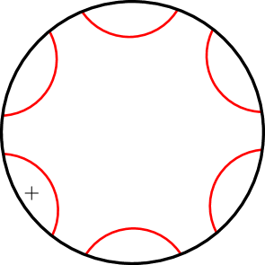
Figure 3. The unique configuration of dividing set for the case $\operatorname{tb}=-6$ and $\operatorname{rot}=5$.

Thus, the first case in which the configuration of the dividing set is not unique is $\operatorname{tb}=-3$ and $\operatorname{rot}=0$; i.e. the first time in which appears a double stabilization. In this case there are three possible configurations of dividing set. See Figure 4.

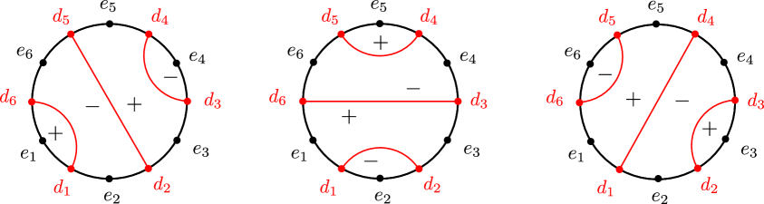
Figure 4. The three possible configurations for $\operatorname{tb}=-3$ and $\operatorname{rot}=0$.

4.2. The space of long Legendrian unknots with maximal rotation number in a tight contact $3$-manifold.

We will prove Theorem 1.2.1. Let $(M,\xi)$ be acontact $3$-manifold. Consider the space ${\mathfrak{Leg}}_{(p,v)}^{t,r}(M,\xi)$ be the space of long Legendrian unknots $\gamma$, i.e. $\gamma(0)=p$ and $\gamma^{\prime}(0)=v$, such that $(\operatorname{tb}(\gamma),\operatorname{rot}(\gamma))=(t,r)$.

Before proving Theorem 1.2.1 we will need a couple of preliminary results. Let $\gamma\in{\mathfrak{Leg}}_{(p,v)}^{t,r}(M,\xi)$ be any Legendrian unknot and consider an embedding $e:{\mathbb{D}}^{2}\rightarrow(M,\xi)$ of a convex Seifert disk for $\gamma$ such that $e(1,0)=\gamma(0)$. Denote by $\mathcal{F}=e^{*}\xi$ the characteristic foliation of $e$. Consider the space ${\mathfrak{Emb}}({\mathbb{D}}^{2},(M,\xi),\mathcal{F};\frac{1}{2}\partial)$ the space of convex embeddings of disks with characteristic foliation $\mathcal{F}$ bounding a long Legendrian unknot with formal invariant $(t,r)$ and that coincides with $e$ on an open neighbourhood of $(1,0)\in{\mathbb{D}}^{2}$. Consider also the subspace ${\mathfrak{Emb}}({\mathbb{D}}^{2},(M,\xi),\mathcal{F})\subseteq{\mathfrak{Emb}}({\mathbb{D}}^{2},(M,\xi),\mathcal{F};\frac{1}{2}\partial)$ of disk embeddings that coincide with $e$ on an open neighbourhood of $\partial{\mathbb{D}}^{2}$. Observe that these spaces fit into a fibration

$${\mathfrak{Emb}}({\mathbb{D}}^{2},(M,\xi),\mathcal{F})\rightarrow{\mathfrak{Emb}}({\mathbb{D}}^{2},(M,\xi),\mathcal{F};\frac{1}{2}\partial)\rightarrow{\mathfrak{Leg}}_{(p,v)}^{t,r}(M,\xi).$$

The first step is to observe that the space of (tight) convex disks with half-boundary fixed is contractible for any Seifert disk of any unknot. That is the content of the following result.

Lemma 4.2.1.

The space ${\mathfrak{Emb}}(({\mathbb{D}}^{2},\mathcal{F}),(M,\xi);\frac{1}{2}\partial)$ is contractible. Hence, there is a homotopy equivalence

$$\Omega{\mathfrak{Leg}}_{(p,v)}^{t,r}(M,\xi)\cong{\mathfrak{Emb}}(({\mathbb{D}}^{2},\mathcal{F}),(M,\xi)).$$

Proof.

Let $\hat{e}:{\mathbb{S}}^{2}\rightarrow(M,\xi)$ be the convex sphere obtained by gluing (and rounding the corners) a copy of $e({\mathbb{D}}^{2})$ with itself in a vertically invariant neighbourhood of the disk. Denote by $\mathcal{F}_{2}=\hat{e}^{*}\xi$ the characteristic foliation of $\hat{e}$ and consider the space ${\mathfrak{Emb}}(({\mathbb{S}}^{2},\mathcal{F}_{2}),(M,\xi))$ of embeddings of convex spheres with characteristic foliation $\mathcal{F}_{2}$ into $(M,\xi)$ that are constant in an open neighbourhood of $e(1,0)$ and also bound a $3$-ball. As explained in Subsection 3.2.7 the space ${\mathfrak{Emb}}(({\mathbb{S}}^{2},\mathcal{F}_{2}),(M,\xi))$ is contractible. Since the space ${\mathfrak{Emb}}(({\mathbb{S}}^{2},\mathcal{F}_{2}),(M,\xi))$ fibers over ${\mathfrak{Emb}}(({\mathbb{D}}^{2},\mathcal{F}),(M,\xi);\frac{1}{2}\partial)$ by restriction over one hemisphere and the fiber is also contractible the result follows. ∎

Proof of Theorem 1.2.1.

The proof follows directly from the previous Lemma and Theorems 3.2.2 and 3.2.4. ∎

4.3. The transverse unknot with self-linking number -1.

It follows from the density of the space of mini-disks (Seifert disks for the transverse unknot with self-linking number $-1$) that the space of long transverse unknots with self-linking number $-1$ has also the same homotopy type that the space of long smooth unknots. We will denote by ${\mathfrak{Trans}}_{(p,v)}^{0}(M,\xi)$ the space of long (positive) transverse unknots with self-linking number. Do note that now $v\in TM$ is transverse and not Legendrian.

Theorem 4.3.1.

If $(M,\xi)$ is tight then the natural inclusion

$${\mathfrak{Trans}}_{(p,v)}^{0}(M,\xi)\hookrightarrow{\mathfrak{Emb}}_{(p,v)}^{0}({\mathbb{S}}^{1},M)$$

is a equivalence.

In particular, for the standard tight $({\mathbb{S}}^{3},\xi_{\operatorname{std}})$ we obtain that

Corollary 4.3.2.

The natural inclusion of the space pf parametrized transverse great circles into the space of embeddings ${\mathfrak{Trans}}^{0}({\mathbb{S}}^{3},\xi_{\operatorname{std}})$ of transverse unknots with self-linking number $-1$ is a homotopy equivalence.

To deduce the statement from the first one realize that there is a fibration

$${\mathfrak{Trans}}_{N,iN}({\mathbb{S}}^{3},\xi_{\operatorname{std}})\hookrightarrow{\mathfrak{Trans}}({\mathbb{S}}^{3},\xi_{\operatorname{std}})\rightarrow{\mathbb{S}}^{3}=\operatorname{SU}(2),$$

in which the fiber is contractible because of the previous Theorem and Theorem 2.5.4. The proof of the result above follows the very same lines as the one that we have provided for the Legendrian unknot with maximal rotation number. We will left the details for the interested reader.

5. Applications.

Let us apply the techniques developed in this article to prove several applications.

5.1. The standard tight $({\mathbb{S}}^{1}\times{\mathbb{S}}^{2},\xi_{\operatorname{std}})$.

We prove Theorem 1.1.3; i.e. we compute the homotopy type of the contactomorphism group of the standard tight $({\mathbb{S}}^{1}\times{\mathbb{S}}^{2},\xi_{\operatorname{std}})$. Let us note the path-connected components of the of the contactomorphism group was studied by Ding and Geiges in [DG10] and completely determined by Hyunki in [Min22]. The main ingredient that we will use is Theorem 3.2.6.

We begin with a Lemma

Lemma 5.1.1.

Let $e:{\mathbb{S}}^{2}\hookrightarrow\{0\}\times{\mathbb{S}}^{2}\subseteq({\mathbb{S}}^{1}\times{\mathbb{S}}^{2},\xi_{\operatorname{std}})$ be the standard convex inclusion. Then, the space ${\mathfrak{Emb}}^{e}_{\operatorname{std}}({\mathbb{S}}^{2},({\mathbb{S}}^{1}\times{\mathbb{S}}^{2},\xi_{\operatorname{std}}))$ is homotopy equivalent to ${\mathbb{S}}^{1}\times\operatorname{U}(1)$.

Proof.

The space ${\mathfrak{Emb}}^{e}({\mathbb{S}}^{2},{\mathbb{S}}^{1}\times{\mathbb{S}}^{2})$ is homotopy equivalent to ${\mathbb{S}}^{1}\times\operatorname{SO}(3)$. This follows from Hatcher’s computation of the homotopy type of the diffeomorphism group of ${\mathbb{S}}^{1}\times{\mathbb{S}}^{2}$ (see [Hat81]). Consider the following commutative diagram

The statement now follows easily from Theorem 3.2.6 and the Five Lemma. ∎

Proof of Theorem 1.1.3.

Let $\mathcal{S}_{\operatorname{std}}$ be the space of embeddings of essential standard spheres into $({\mathbb{S}}^{1}\times{\mathbb{S}}^{2},\xi_{\operatorname{std}})$ and $\mathcal{S}$ be its smooth counterpart. Do note that $\mathcal{S}$ has exactly to path–connected components, the one containing $e:{\mathbb{S}}^{2}\rightarrow\{0\}\times{\mathbb{S}}^{2}$ and the one containing $e\circ A$, where $A:{\mathbb{S}}^{2}\rightarrow{\mathbb{S}}^{2}$ denotes the antipodal map. Observe that an standard convex sphere has an antipodal symmetry so $e\circ A$ is standard. Moreover, it follows from the work of Colin [Col97] that the inclusion $\mathcal{S}_{\operatorname{std}}\hookrightarrow\mathcal{S}$ induces an isomorphism on $\pi_{0}$; therefore we conclude that

$$\mathcal{S}_{\operatorname{std}}={\mathfrak{Emb}}^{e}_{\operatorname{std}}({\mathbb{S}}^{2},({\mathbb{S}}^{1}\times{\mathbb{S}}^{2},\xi_{\operatorname{std}}))\cup{\mathfrak{Emb}}^{e\circ A}_{\operatorname{std}}({\mathbb{S}}^{2},({\mathbb{S}}^{1}\times{\mathbb{S}}^{2},\xi_{\operatorname{std}})).$$

In particular, because of the previous Lemma we see that the natural inclusion ${\mathbb{S}}^{1}\times\operatorname{O}(2)\hookrightarrow\mathcal{S}_{\operatorname{std}}$ is a homotopy equivalence.

Consider the fiber bundle

$$\operatorname{Cont}({\mathbb{S}}^{2}\times I,\xi_{\operatorname{std}})\hookrightarrow\operatorname{Cont}({\mathbb{S}}^{1}\times{\mathbb{S}}^{2},\xi_{\operatorname{std}})\rightarrow\mathcal{S}_{\operatorname{std}}.$$

Defined by acting by postcomposition with a contactomorphism over the embedding $e$. Note also that the fiber bundle projection is surjective. Indeed, the diffeomorphism of $\varphi_{A}:{\mathbb{S}}^{1}\times{\mathbb{S}}^{2}\rightarrow{\mathbb{S}}^{1}\times{\mathbb{S}}^{2},(\theta,p)\mapsto(-\theta,A(p))$, is a contactomorphism.

Finally, recall that we have proved in Corollary 3.1.4 that there is an inclusion $\Omega\operatorname{U}(1)\hookrightarrow\operatorname{Cont}({\mathbb{S}}^{2}\times I,\xi_{\operatorname{std}})$ which induces a homotopy equivalence . Thus, the natural inclusion ${\mathbb{S}}^{1}\times\operatorname{O}(2)\times\Omega\operatorname{U}(1)\hookrightarrow\operatorname{Cont}({\mathbb{S}}^{1}\times{\mathbb{S}}^{2},\xi_{\operatorname{std}})$ fits in the map of fibrations

$$\lx@xy@svg{\hbox{\raise 0.0pt\hbox{\kern 48.2056pt\hbox{\ignorespaces\ignorespaces\ignorespaces\hbox{\vtop{\kern 0.0pt\offinterlineskip\halign{\entry@#!@&&\entry@@#!@\cr&\\&\\&\crcr}}}\ignorespaces{\hbox{\kern-23.75003pt\raise 0.0pt\hbox{\hbox{\kern 0.0pt\raise 0.0pt\hbox{\hbox{\kern 10.0pt\raise 0.0pt\hbox{$\textstyle{\Omega\operatorname{U}(1)\ignorespaces\ignorespaces\ignorespaces\ignorespaces\ignorespaces\ignorespaces\ignorespaces\ignorespaces}$}}}}}}}\ignorespaces\ignorespaces\ignorespaces\ignorespaces{\hbox{\kern 23.75003pt\raise 0.0pt\hbox{\hbox{\kern 0.0pt\raise 0.0pt\hbox{\lx@xy@hook{1}}}}}}{\hbox{\lx@xy@droprule}}\ignorespaces{\hbox{\kern 72.68204pt\raise 0.0pt\hbox{\hbox{\kern 0.0pt\raise 0.0pt\hbox{\lx@xy@tip{1}\lx@xy@tip{-1}}}}}}{\hbox{\lx@xy@droprule}}{\hbox{\lx@xy@droprule}}\ignorespaces\ignorespaces\ignorespaces\ignorespaces{\hbox{\kern 0.0pt\raise-12.5pt\hbox{\hbox{\kern 0.0pt\raise 0.0pt\hbox{\lx@xy@hook{1}}}}}}{\hbox{\lx@xy@droprule}}\ignorespaces{\hbox{\kern 0.0pt\raise-36.5pt\hbox{\hbox{\kern 0.0pt\raise 0.0pt\hbox{\lx@xy@tip{1}\lx@xy@tip{-1}}}}}}{\hbox{\lx@xy@droprule}}{\hbox{\lx@xy@droprule}}{\hbox{\kern 72.68204pt\raise 0.0pt\hbox{\hbox{\kern 0.0pt\raise 0.0pt\hbox{\hbox{\kern 10.0pt\raise 0.0pt\hbox{$\textstyle{\operatorname{Cont}({\mathbb{S}}^{2}\times I,\xi_{\operatorname{std}})\ignorespaces\ignorespaces\ignorespaces\ignorespaces}$}}}}}}}\ignorespaces\ignorespaces\ignorespaces\ignorespaces{\hbox{\kern 117.19205pt\raise-12.5pt\hbox{\hbox{\kern 0.0pt\raise 0.0pt\hbox{\lx@xy@hook{1}}}}}}{\hbox{\lx@xy@droprule}}\ignorespaces{\hbox{\kern 117.19205pt\raise-36.5pt\hbox{\hbox{\kern 0.0pt\raise 0.0pt\hbox{\lx@xy@tip{1}\lx@xy@tip{-1}}}}}}{\hbox{\lx@xy@droprule}}{\hbox{\lx@xy@droprule}}{\hbox{\kern-48.2056pt\raise-55.13776pt\hbox{\hbox{\kern 0.0pt\raise 0.0pt\hbox{\hbox{\kern 10.0pt\raise 0.0pt\hbox{$\textstyle{{\mathbb{S}}^{1}\times\operatorname{O}(2)\times\Omega\operatorname{U}(1)\ignorespaces\ignorespaces\ignorespaces\ignorespaces\ignorespaces\ignorespaces\ignorespaces\ignorespaces}$}}}}}}}\ignorespaces\ignorespaces\ignorespaces\ignorespaces{\hbox{\kern 48.2056pt\raise-55.13776pt\hbox{\hbox{\kern 0.0pt\raise 0.0pt\hbox{\lx@xy@hook{1}}}}}}{\hbox{\lx@xy@droprule}}\ignorespaces{\hbox{\kern 72.2056pt\raise-55.13776pt\hbox{\hbox{\kern 0.0pt\raise 0.0pt\hbox{\lx@xy@tip{1}\lx@xy@tip{-1}}}}}}{\hbox{\lx@xy@droprule}}{\hbox{\lx@xy@droprule}}\ignorespaces\ignorespaces\ignorespaces\ignorespaces{}{\hbox{\lx@xy@droprule}}\ignorespaces{\hbox{\kern 0.0pt\raise-91.63776pt\hbox{\hbox{\kern 0.0pt\raise 0.0pt\hbox{\lx@xy@tip{1}\lx@xy@tip{-1}}}}}}{\hbox{\lx@xy@droprule}}{\hbox{\lx@xy@droprule}}{\hbox{\kern 72.2056pt\raise-55.13776pt\hbox{\hbox{\kern 0.0pt\raise 0.0pt\hbox{\hbox{\kern 10.0pt\raise 0.0pt\hbox{$\textstyle{\operatorname{Cont}({\mathbb{S}}^{1}\times{\mathbb{S}}^{2},\xi_{\operatorname{std}})\ignorespaces\ignorespaces\ignorespaces\ignorespaces}$}}}}}}}\ignorespaces\ignorespaces\ignorespaces\ignorespaces{}{\hbox{\lx@xy@droprule}}\ignorespaces{\hbox{\kern 117.19205pt\raise-93.4422pt\hbox{\hbox{\kern 0.0pt\raise 0.0pt\hbox{\lx@xy@tip{1}\lx@xy@tip{-1}}}}}}{\hbox{\lx@xy@droprule}}{\hbox{\lx@xy@droprule}}{\hbox{\kern-28.3445pt\raise-110.27551pt\hbox{\hbox{\kern 0.0pt\raise 0.0pt\hbox{\hbox{\kern 10.0pt\raise 0.0pt\hbox{$\textstyle{{\mathbb{S}}^{1}\times\operatorname{O}(2)\ignorespaces\ignorespaces\ignorespaces\ignorespaces}$}}}}}}}\ignorespaces\ignorespaces\ignorespaces\ignorespaces{\hbox{\kern 28.3445pt\raise-110.27551pt\hbox{\hbox{\kern 0.0pt\raise 0.0pt\hbox{\lx@xy@hook{1}}}}}}{\hbox{\lx@xy@droprule}}\ignorespaces{\hbox{\kern 100.66537pt\raise-110.27551pt\hbox{\hbox{\kern 0.0pt\raise 0.0pt\hbox{\lx@xy@tip{1}\lx@xy@tip{-1}}}}}}{\hbox{\lx@xy@droprule}}{\hbox{\lx@xy@droprule}}{\hbox{\kern 100.66537pt\raise-110.27551pt\hbox{\hbox{\kern 0.0pt\raise 0.0pt\hbox{\hbox{\kern 10.0pt\raise 0.0pt\hbox{$\textstyle{\mathcal{S}_{\operatorname{std}}}$}}}}}}}\ignorespaces}}}}\ignorespaces, \textstyle{\Omega\operatorname{U}(1)\ignorespaces\ignorespaces\ignorespaces\ignorespaces\ignorespaces\ignorespaces\ignorespaces\ignorespaces} \textstyle{\operatorname{Cont}({\mathbb{S}}^{2}\times I,\xi_{\operatorname{std}})\ignorespaces\ignorespaces\ignorespaces\ignorespaces} \textstyle{{\mathbb{S}}^{1}\times\operatorname{O}(2)\times\Omega\operatorname{U}(1)\ignorespaces\ignorespaces\ignorespaces\ignorespaces\ignorespaces\ignorespaces\ignorespaces\ignorespaces} \textstyle{\operatorname{Cont}({\mathbb{S}}^{1}\times{\mathbb{S}}^{2},\xi_{\operatorname{std}})\ignorespaces\ignorespaces\ignorespaces\ignorespaces} \textstyle{{\mathbb{S}}^{1}\times\operatorname{O}(2)\ignorespaces\ignorespaces\ignorespaces\ignorespaces} \textstyle{\mathcal{S}_{\operatorname{std}}} \textstyle{\Omega\operatorname{U}(1)\ignorespaces\ignorespaces\ignorespaces\ignorespaces\ignorespaces\ignorespaces\ignorespaces\ignorespaces} \textstyle{\operatorname{Cont}({\mathbb{S}}^{2}\times I,\xi_{\operatorname{std}})\ignorespaces\ignorespaces\ignorespaces\ignorespaces} \textstyle{{\mathbb{S}}^{1}\times\operatorname{O}(2)\times\Omega\operatorname{U}(1)\ignorespaces\ignorespaces\ignorespaces\ignorespaces\ignorespaces\ignorespaces\ignorespaces\ignorespaces} \textstyle{\operatorname{Cont}({\mathbb{S}}^{1}\times{\mathbb{S}}^{2},\xi_{\operatorname{std}})\ignorespaces\ignorespaces\ignorespaces\ignorespaces} \textstyle{{\mathbb{S}}^{1}\times\operatorname{O}(2)\ignorespaces\ignorespaces\ignorespaces\ignorespaces} \textstyle{\mathcal{S}_{\operatorname{std}}}$$

where the maps between the base and the fibers are homotopy equivalences. Thus, the map between the total spaces of the fibrations is a homotopy equivalence.

To deduce the second statement use the fiber bundle

$$\operatorname{Cont}_{0}({\mathbb{S}}^{1}\times{\mathbb{S}}^{2},\xi_{\operatorname{std}})\rightarrow\operatorname{Diff}_{0}({\mathbb{S}}^{1}\times{\mathbb{S}}^{2})\rightarrow{\mathfrak{C}Str}({\mathbb{S}}^{1}\times{\mathbb{S}}^{2};\xi_{\operatorname{std}}),$$

where $\operatorname{Diff}_{0}({\mathbb{S}}^{1}\times{\mathbb{S}}^{2})$ is the path connected component of the identity inside $\operatorname{Diff}({\mathbb{S}}^{1}\times{\mathbb{S}}^{2})$ and $\operatorname{Cont}_{0}({\mathbb{S}}^{1}\times{\mathbb{S}}^{2},\xi_{\operatorname{std}})=\operatorname{Diff}_{0}({\mathbb{S}}^{1}\times{\mathbb{S}}^{2})\cap\operatorname{Cont}({\mathbb{S}}^{1}\times{\mathbb{S}}^{2},\xi_{\operatorname{std}})$. The space $\operatorname{Diff}_{0}({\mathbb{S}}^{1}\times{\mathbb{S}}^{2})$ is homotopy equivalent to ${\mathbb{S}}^{1}\times\operatorname{SO}(3)\times\Omega^{0}\operatorname{SO}(3)$ by [Hat81] and we have just proved that $\operatorname{Cont}_{0}({\mathbb{S}}^{1}\times{\mathbb{S}}^{2},\xi_{\operatorname{std}})$ is homotopy equivalent to ${\mathbb{S}}^{1}\times\operatorname{U}(1)\times\Omega^{\operatorname{even}}\operatorname{U}(1)$. Here $\Omega^{0}\operatorname{SO}(3)$ denotes the subspace of $\Omega\operatorname{SO}(3)$ of contractible loops and $\Omega^{\operatorname{even}}\operatorname{U}(1)$ the subspace of loops in $\operatorname{U}(1)$ that are contractible inside $\operatorname{SO}(3)$. ∎

5.2. Legendrian circles bundles over surfaces with boundary.

We prove Theorem 1.1.4. Recall that we have proven in Corollary 3.3.3 that the inclusion of the diffeomorphism group of the $2$-disk into the contactomorphism group of the space of cooriented contact elements over a disk is a homotopy equivalence, which is a particular case of the result. Let $(V,\xi)$ be any Legendrian fibration over a compact orientable surface with non-empty boundary $S$. Consider the natural inclusion

$$i:\operatorname{Diff}(S)\hookrightarrow\operatorname{Cont}(V,\xi).$$

We will use the microfibration argument to mimic the proof given by Giroux and Massot [GM17] in the $\pi_{0}$-case. The beautiful proof given by Giroux and Massot for the $\pi_{0}$ statement is based on reducing the complexity of the $3$-manifold $V$ by cutting $V$ over an annulus fibered over properly embedding non-separating arcs and applying an inductive argument.

More precisely, let $e:A\hookrightarrow(V,\xi)$ a convex embedding of an annulus fibered over a non-separating properly embedded arc on $S$. Do note that the characteristic foliation of the annulus $A$ is given by the Legendrian fibers (rullings) and $2d$ transversing Legendrian divides (parallel to the arc over which the annulus is fibered), between each Legendrian divide there is a dividing curve. We denote by ${\mathfrak{Emb}}^{e}(A,V)$ the space of smooth embeddings that coincide with $e$ near the boundary and are isotopic to $e$. Denote also by ${\mathfrak{Emb}}_{\operatorname{std}}^{e}(A,(V,\xi))\subseteq{\mathfrak{Emb}}^{e}(A,V)$ the subspace of convex embeddings with the same characteristic foliation than $e$. The argument given in [GM17] to check the injectivity of $i$ on $\pi_{0}$ was based on proving first the $\pi_{0}$-injectivity of the map

$$j:\operatorname{Cont}(V,\xi)\hookrightarrow\operatorname{Diff}(V)$$

from which one can deduce the isomorphism on $\pi_{0}$ stated above. To prove the $\pi_{0}$-injectivity of $j$ they proved that the inclusion ${\mathfrak{Emb}}_{\operatorname{std}}^{e}(A,(V,\xi))\hookrightarrow{\mathfrak{Emb}}^{e}(A,V)$ is $\pi_{0}$ injective, even more, the relative homotopy group $\pi_{1}({\mathfrak{Emb}}^{e}(A,V),{\mathfrak{Emb}}_{\operatorname{std}}^{e}(A,(V,\xi)))=0$. This allowed them to induct on the number

$$n(S)=-2\chi(S)-\beta(S)=\beta(S)+4g(S)-4,$$

where $g(S)$ is the genus of $S$ and $\beta(S)$ the number of boundary components. The base case is when $n(S)=-3$, i.e. when $S$ is a disk. For this case the statement follows from Colin’s argument [Col97] applied to standard disks, see Giroux [Gir01b]. Do note, that we have already proved the parametric version of the base case in Corollary 3.3.3. Therefore, what remains to conclude is to study the inclusion ${\mathfrak{Emb}}_{\operatorname{std}}^{e}(A,(V,\xi))\hookrightarrow{\mathfrak{Emb}}^{e}(A,V)$ in a multiparametric fashion. That is the content of the following result:

Lemma 5.2.1.

The inclusion ${\mathfrak{Emb}}_{\operatorname{std}}^{e}(A,(V,\xi))\hookrightarrow{\mathfrak{Emb}}^{e}(A,V)$ is a homotopy equivalence.

Proof.

We will make use of the microfibration trick to prove this statement. In order to do that we should

• Prove the statement locally (in a neighbourhood) of $e(A)$.

• Prove that the space of standard embeddings smoothly isotopic to $e$ is $C^{0}$-dense into the space of smooth embeddings isotopic to $e$.

The second property (ii) was actually proved by Giroux and Massot [GM17] in Proposition 2.4. and follows from the fact that the Legendrian fiber cannot be destabilized. It is left to check (i). Let $U$ be an small tubular neighbourhood of $A$ (do note that $U$ is a solid tori). Since $A$ is convex we may take $U$ as an $I$-invariant neighbourhood. Moreover, it follows that $(U,\xi)$ is a standard solid torus. Therefore, in the following commutative diagram

the map inclusion between the fibers and the total spaces are homotopy equivalences (Theorem 3.3.2, therefore the map between the bases is a homotopy equivalence. Apply the microfibration argument to conclude. ∎

Proof of Theorem 1.1.4.

Recall that the components of $\operatorname{Diff}(S)$ and $\operatorname{Diff}(V)$ are contractible (see [ES70, Gra73, Iva76, Hat76, Hat99a]). Therefore, it is enough to prove that the inclusion

$$\operatorname{Cont}(V,\xi)\hookrightarrow\operatorname{Diff}(V)$$

induces an isomorphism on $\pi_{k}$, for every $k>0$, and invoke [GM17] for the $\pi_{0}$-case. We will proceed by induction on $n(S)$. The base case was already proved so, let’s assume that $n(S)>3$. The proof follows from the previous Lemma by considering the commutative diagram

in which the subscript $0$ means isotopic (and therefore contact isotopic) to the identity. Here $(V^{\prime},\xi)$ is a Legendrian circle bundle over a surface $S^{\prime}$ for which

$$n(S^{\prime})<n(S).$$

It follows from the previous Lemma that the map between the bases is a homotopy equivalence. Therefore, we deduce that there are natural isomorphisms

$$\pi_{k}(\operatorname{Diff}_{0}(V),\operatorname{Cont}_{0}(V,\xi))\cong\pi_{k}(\operatorname{Diff}_{0}(V^{\prime}),\operatorname{Cont}_{0}(V^{\prime},\xi))$$

for every $k>0$. Apply the induction hypothesis to conclude. ∎

5.3. The space of Legendrian parametrized $(n,n)$-torus links with max-$\operatorname{tb}$.

We prove Theorem 1.2.4. Recall that $\mathcal{L}_{n}$ denotes the space of Legendrian embeddings

$$\gamma=\sqcup_{i=1}^{n}\gamma_{i}:\sqcup_{i=1}^{N}{\mathbb{S}}^{1}\rightarrow({\mathbb{S}}^{3},\xi_{\operatorname{std}})$$

of $(n,n)$-torus links with maximal $\operatorname{tb}$. For instance, $\mathcal{L}_{1}$ is the space of embeddings of the standard Legendrian unknot and $\mathcal{L}_{2}$ the space of embeddings of the standard Legendrian Hopf link. For $n>0$ denote by $S_{n}$ the $2$-sphere ${\mathbb{S}}^{2}$ with $n$ holes and, similarly, by $D_{n}$ the $2$-disk ${\mathbb{D}}^{2}$ with $n$ holes.

Proof of Theorem 1.2.4.

Any Legendrian $(n,n)$-torus link can be regarded as $n$ distinct parametrized fibers of the Legendrian fibration $({\mathbb{S}}^{3},\xi_{\operatorname{std}})\rightarrow{\mathbb{C}}{\mathbb{P}}^{1}$ induced by the $j$-complex structure on ${\mathbb{R}}^{4}$. The main geometric observation is that the $(n-1,n-1)$-torus link $\hat{\gamma}=\sqcup_{i=2}^{N-1}\gamma_{i}$ which lies in the complement of the Legendrian unknot $\gamma_{1}$ can be regarded as $(n-1)$ distinct Legendrian fibers of the Legendrian fibration $({\mathbb{S}}(T^{*}{\mathbb{D}}^{2}),\lambda_{\operatorname{std}})\cong({\mathbb{S}}^{3}\backslash\gamma_{1}({\mathbb{S}}^{1}),\xi_{\operatorname{std}})$.

As usual there is a homotopy equivalence

$$\mathcal{L}_{n}\cong\operatorname{U}(2)\times\mathcal{L}^{\prime}_{n},$$

where $\mathcal{L}^{\prime}_{n}$ is the subspace of Legendrian links $\gamma=\sqcup_{i=1}^{n}\gamma_{i}$ such that $\gamma_{1}(0)=N$ and $\gamma^{\prime}_{1}(N)=jN$. Thus, it is enough to check that there is a homotopy equivalence between $\mathcal{L}^{\prime}_{n}$ and a $K(\mathcal{M}_{n},1)$.

Consider the fibration

$$\operatorname{Cont}({\mathbb{D}}^{3},\xi_{\operatorname{std}})\rightarrow\mathcal{L}^{\prime}_{n}.$$

The fiber over any Legendrian link $\gamma$ can be identified with

$$\operatorname{Cont}({\mathbb{S}}(T^{*}D_{n-1}),\lambda_{\operatorname{std}})=\operatorname{Cont}({\mathbb{S}}(T^{*}{\mathbb{D}}^{2}),\lambda_{\operatorname{std}};\operatorname{rel}\hat{\gamma}(\sqcup_{i=2}^{n}{\mathbb{S}}^{1})).$$

Since $\operatorname{Cont}({\mathbb{D}}^{3},\xi_{\operatorname{std}})$ is contractible by Corollary 3.1.4 there is a homotopy equivalence

$$\operatorname{Cont}({\mathbb{S}}(T^{*}D_{n-1}),\lambda_{\operatorname{std}})\cong\Omega\mathcal{L}^{\prime}_{n}.$$

Finally, apply Theorem 1.1.4 to conclude that the inclusion

$$\operatorname{Diff}(D_{n-1})\hookrightarrow\operatorname{Cont}({\mathbb{S}}(T^{*}D_{n-1}),\lambda_{\operatorname{std}})$$

is a homotopy equivalence. Observe that the groups $\operatorname{Diff}(D_{n-1})$ and $\operatorname{Diff}(S_{n})$ coincide and are homotopically discrete. Thus, the result follows since

$$\Omega\mathcal{L}^{\prime}_{n}\cong\operatorname{Cont}({\mathbb{S}}(T^{*}D_{n-1}),\lambda_{\operatorname{std}})\cong\operatorname{Diff}(S_{n})$$

and

$$\mathcal{M}_{n}=\pi_{0}(\operatorname{Diff}(S_{n}))$$

by definition. ∎

5.4. Parametric families of tight charts.

Denote by $\operatorname{Tight}({\mathbb{R}}^{3})$ the space of tight contact structures on ${\mathbb{R}}^{3}$. A celebrated Theorem of Eliashberg [Eli92] states that for every $\xi\in\operatorname{Tight}({\mathbb{R}}^{3})$ there exists a contactomorphism $\varphi:({\mathbb{R}}^{3},\xi)\rightarrow({\mathbb{R}}^{3},\xi_{\operatorname{std}})$. We will prove this parametric version that generalizes it:

Theorem 5.4.1.

Let $\xi^{z}\in\operatorname{Tight}({\mathbb{R}}^{3})$, $z\in K$, be a continuous compact family of tight contact structures on ${\mathbb{R}}^{3}$, such that there is a choice of contact form $\alpha_{z}$ at ${\mathcal{O}p}(0)$ for which the Reeb field satisfies $R_{z}(0)=\partial_{z}$. Then, there exists a continuous family of contactomorphisms $\varphi_{z}:({\mathbb{R}}^{3},\xi^{z})\rightarrow({\mathbb{R}}^{3},\xi_{\operatorname{std}})$.

Proof.

The condition at the origin immediately implies that $\xi^{z}$ may be chosen fixed at ${\mathcal{O}p}(0)$. Since the space of contact structures that we are considering retracts by Alexander’s trick to the standard contact structure, we may consider that we have a cone of tight contact structures $\xi^{z,t}$, $(z,t)\in K\times[0,1]$, for which we obtain $\xi^{z,1}=\xi^{z}$ and $\xi^{z,0}=\xi_{\operatorname{std}}$.

Fix the ray $\lambda=\{x=y=0,z>0\}$ and consider the exhaustion ${\mathbb{R}}^{3}=\cup_{n}{\mathbb{D}}^{3}(n)$. Observe that ${\mathbb{S}}_{n}^{2}=\partial{\mathbb{D}}^{3}(n)$ is convex for the standard contact structure $({\mathbb{R}}^{3},\xi_{\operatorname{std}})$ and in view of Theorem 3.2.6, we can easily find a parametric family of embeddings of $e_{z,t,n}$ spheres that are standard for $\xi^{z,t}$ and close in Haussdorf distance to the embedding ${\mathbb{S}}^{2}(n)\times\{n\}$. Moreover, we can make sure that they keep ${\mathbb{S}}^{2}\bigcap\lambda$ fixed and the characteristic foliation at that point possesses the positive elliptic singularity. This is precisely the statement of Theorem 3.2.6. Recall that $e_{z,t,n}$ is isotopic to $e_{0}$ through smooth spheres, so by extension of isotopy we define a global diffeomorphism $F_{z,t,n}$ on ${\mathbb{R}}^{3}$ that satisfies $e_{z,t,n}=F_{z,t,n}\circ e_{0}$ with very small support. In particular, for every pair of positive integers $m\neq n$ the supports of $F_{z,t,n}$ and $F_{z,t,m}$ are disjoint. Thus, define $F_{z,t}=F_{z,t,1}\circ F_{z,t,2}\circ\cdots$ that is a diffeomorphism such that $F_{z,t}\circ e_{0,n}$ is a standard embedding and moreover it is a contactomorphism on a small open neighborhood, i.e. $F_{z,t}^{*}\xi^{z,t}=\xi^{{\operatorname{std}}}$ for the domain $\bigcup_{n\in{\mathbb{Z}}^{+}}{\mathcal{O}p}({\mathbb{S}}^{2}(n))$. Even more, we may assume at the beginning that $e_{z,0,n}=e$ and $F_{z,0}={\operatorname{Id}}$. Therefore, there is a $1$-parametric family $\xi^{z,t}$ of contact structures, i.e. we consider $t$ as the time and $z\in K$ a fixed parameter. To apply Gray’s Theorem we need to make sure that Gray’s flow is complete. But this is the case because the contact structures coincide in the family of spheres ${\mathbb{S}}^{2}(n)$ and this forces the Gray flow to remain confined in the complementary annuli. Thus, there exists a family $G^{z,t}$ of diffeomorphisms satisfying that $G^{z,t}_{*}\xi^{z,0}=\xi^{z,t}$. Composing we obtain that $F^{z,t}\circ G^{z,t}$ is the required contactomorphism. ∎

References

- [BEM15] Matthew Strom Borman, Yakov Eliashberg, and Emmy Murphy. Existence and classification of overtwisted contact structures in all dimensions. Acta Math., 215(2):281–361, 2015.
- [Ben83] Daniel Bennequin. Entrelacements et équations de Pfaff. In Third Schnepfenried geometry conference, Vol. 1 (Schnepfenried, 1982), volume 107 of Astérisque, pages 87–161. Soc. Math. France, Paris, 1983.
- [BK17] Richard H Bamler and Bruce Kleiner. Ricci flow and diffeomorphism groups of 3-manifolds. arXiv, pages arXiv–1712, 2017.
- [BK21] Richard H. Bamler and Bruce Kleiner. Diffeomorphism groups of prime 3-manifolds, 2021.
- [Bou06] Frédéric Bourgeois. Contact homology and homotopy groups of the space of contact structures. Math. Res. Lett., 13(1):71–85, 2006.
- [Bud10] Ryan Budney. Topology of knot spaces in dimension 3. Proc. Lond. Math. Soc. (3), 101(2):477–496, 2010.
- [CDRGG15] Baptiste Chantraine, Georgios Dimitroglou Rizell, Paolo Ghiggini, and Roman Golovko. Floer homology and Lagrangian concordance. In Proceedings of the Gökova Geometry-Topology Conference 2014, pages 76–113. Gökova Geometry/Topology Conference (GGT), Gökova, 2015.
- [CG22] Roger Casals and Honghao Gao. Infinitely many Lagrangian fillings. Ann. of Math. (2), 195(1):207–249, 2022.
- [CGH09] Vincent Colin, Emmanuel Giroux, and Ko Honda. Finitude homotopique et isotopique des structures de contact tendues. Publ. Math. Inst. Hautes Études Sci., (109):245–293, 2009.
- [Che02] Yuri Chekanov. Differential algebra of Legendrian links. Invent. Math., 150(3):441–483, 2002.
- [CN13] Wutichai Chongchitmate and Lenhard Ng. An atlas of Legendrian knots. Exp. Math., 22(1):26–37, 2013.
- [Col97] Vincent Colin. Chirurgies d’indice un et isotopies de sphères dans les variétés de contact tendues. C. R. Acad. Sci. Paris Sér. I Math., 324(6):659–663, 1997.
- [Col99] Vincent Colin. Recollement de variétés de contact tendues. Bull. Soc. Math. France, 127(1):43–69, 1999.
- [Col08] Vincent Colin. Livres ouverts en géométrie de contact (d’après Emmanuel Giroux). Number 317, pages Exp. No. 969, vii, 91–117. 2008. Séminaire Bourbaki. Vol. 2006/2007.
- [CP14] Roger Casals and Francisco Presas. A remark on the Reeb flow for spheres. J. Symplectic Geom., 12(4):657–671, 2014.
- [CPP21] Roger Casals, Dishant M Pancholi, and Francisco Presas. The legendrian whitney trick. Geometry & Topology, 25(6):3229–3256, nov 2021.
- [CS16] Roger Casals and Oldřich Spáčil. Chern-Weil theory and the group of strict contactomorphisms. J. Topol. Anal., 8(1):59–87, 2016.
- [DG07] Fan Ding and Hansjörg Geiges. Legendrian knots and links classified by classical invariants. Commun. Contemp. Math., 9(2):135–162, 2007.
- [DG10] Fan Ding and Hansjörg Geiges. The diffeotopy group of via contact topology. Compos. Math., 146(4):1096–1112, 2010.
- [Dym01] Katarzyna Dymara. Legendrian knots in overtwisted contact structures on . Ann. Global Anal. Geom., 19(3):293–305, 2001.
- [Dym05] Katarzyna Dymara. The Group of Contactomorphisms of the Sphere Fixing an Overtwisted Disk. arXiv Mathematics e-prints, page math/0507444, July 2005.
- [EES07] Tobias Ekholm, John Etnyre, and Michael Sullivan. Legendrian contact homology in . Trans. Amer. Math. Soc., 359(7):3301–3335, 2007.
- [EF09] Yakov Eliashberg and Maia Fraser. Topologically trivial Legendrian knots. J. Symplectic Geom., 7(2):77–127, 2009.
- [EGH00] Y. Eliashberg, A. Givental, and H. Hofer. Introduction to symplectic field theory. Geom. Funct. Anal., (Special Volume, Part II):560–673, 2000. GAFA 2000 (Tel Aviv, 1999).
- [EK] Y. Eliashberg and T. Kragh. Detecting non-trivial elements in the spaces of legendrian knots via algebraic k-theory. In preparation.
- [Eli89] Y. Eliashberg. Classification of overtwisted contact structures on -manifolds. Invent. Math., 98(3):623–637, 1989.
- [Eli92] Yakov Eliashberg. Contact -manifolds twenty years since J. Martinet’s work. Ann. Inst. Fourier (Grenoble), 42(1-2):165–192, 1992.
- [Eli93] Yakov Eliashberg. Legendrian and transversal knots in tight contact -manifolds. In Topological methods in modern mathematics (Stony Brook, NY, 1991), pages 171–193. Publish or Perish, Houston, TX, 1993.
- [EM02] Y. Eliashberg and N. Mishachev. Introduction to the -principle, volume 48 of Graduate Studies in Mathematics. American Mathematical Society, Providence, RI, 2002.
- [EM21] Yakov Eliashberg and Nikolai Mishachev. The space of tight contact structures on is contractible. arXiv e-prints, page arXiv:2108.09452, August 2021.
- [EP96] Y. Eliashberg and L. Polterovich. Local Lagrangian -knots are trivial. Ann. of Math. (2), 144(1):61–76, 1996.
- [EP22] Yakov Eliashberg and Dishant Pancholi. Honda-huang’s work on contact convexity revisited, 2022.
- [ES70] C. J. Earle and A. Schatz. Teichmüller theory for surfaces with boundary. J. Differential Geometry, 4:169–185, 1970.
- [Etn04] John B. Etnyre. Convex surfaces in contact geometry: class notes, July 2004. Available at etnyre.math.gatech.edu/preprints/papers/surfaces.pdf.
- [Etn05] John B. Etnyre. Legendrian and transversal knots. In Handbook of knot theory, pages 105–185. Elsevier B. V., Amsterdam, 2005.
- [FG20] Eduardo Fernández and Fabio Gironella. A remark on the contactomorphism group of overtwisted contact spheres. C. R. Math. Acad. Sci. Paris, 358(2):189–196, 2020.
- [FMAP20] Eduardo Fernández, Javier Martínez-Aguinaga, and Francisco Presas. Fundamental groups of formal Legendrian and horizontal embedding spaces. Algebr. Geom. Topol., 20(7):3219–3312, 2020.
- [Fra96] Maia Fraser. Example of nonisotopic Legendrian curves not distinguished by the invariants and . Internat. Math. Res. Notices, (19):923–928, 1996.
- [Gab01] David Gabai. The Smale conjecture for hyperbolic 3-manifolds: . J. Differential Geom., 58(1):113–149, 2001.
- [Gei08] Hansjörg Geiges. An introduction to contact topology, volume 109 of Cambridge Studies in Advanced Mathematics. Cambridge University Press, Cambridge, 2008.
- [GGP04] Hansjörg Geiges and Jesús Gonzalo Perez. On the topology of the space of contact structures on torus bundles. Bull. London Math. Soc., 36(5):640–646, 2004.
- [Gir91] Emmanuel Giroux. Convexité en topologie de contact. Comment. Math. Helv., 66(4):637–677, 1991.
- [Gir00] Emmanuel Giroux. Structures de contact en dimension trois et bifurcations des feuilletages de surfaces. Invent. Math., 141(3):615–689, 2000.
- [Gir01a] Emmanuel Giroux. Structures de contact sur les variétés fibrées en cercles audessus d’une surface. Comment. Math. Helv., 76(2):218–262, 2001.
- [Gir01b] Emmanuel Giroux. Sur les transformations de contact au-dessus des surfaces. In Essays on geometry and related topics, Vol. 1, 2, volume 38 of Monogr. Enseign. Math., pages 329–350. Enseignement Math., Geneva, 2001.
- [Gir02] Emmanuel Giroux. Géométrie de contact: de la dimension trois vers les dimensions supérieures. In Proceedings of the International Congress of Mathematicians, Vol. II (Beijing, 2002), pages 405–414. Higher Ed. Press, Beijing, 2002.
- [Gir19] Fabio Gironella. Examples of nontrivial contact mapping classes for overtwisted contact manifolds in all dimensions. Algebr. Geom. Topol., 19(3):1207–1227, 2019.
- [Gir21] Fabio Gironella. Examples of contact mapping classes of infinite order in all dimensions. Math. Res. Lett., 28(3):707–727, 2021.
- [GK14] Hansjörg Geiges and Mirko Klukas. The fundamental group of the space of contact structures on the 3-torus. Math. Res. Lett., 21(6):1257–1262, 2014.
- [GM17] Emmanuel Giroux and Patrick Massot. On the contact mapping class group of Legendrian circle bundles. Compos. Math., 153(2):294–312, 2017.
- [Gom98] Robert E. Gompf. Handlebody construction of Stein surfaces. Ann. of Math. (2), 148(2):619–693, 1998.
- [Gra59] John W. Gray. Some global properties of contact structures. Ann. of Math. (2), 69:421–450, 1959.
- [Gra73] André Gramain. Le type d’homotopie du groupe des difféomorphismes d’une surface compacte. Ann. Sci. École Norm. Sup. (4), 6:53–66, 1973.
- [Gro86] Mikhael Gromov. Partial differential relations, volume 9 of Ergebnisse der Mathematik und ihrer Grenzgebiete (3) [Results in Mathematics and Related Areas (3)]. Springer-Verlag, Berlin, 1986.
- [Hat] Allen Hatcher. Topological moduli spaces of knots. Available at pi.math.cornell.edu/ hatcher/Papers/knotspaces.pdf.
- [Hat76] Allen Hatcher. Homeomorphisms of sufficiently large -irreducible -manifolds. Topology, 15(4):343–347, 1976.
- [Hat81] A. Hatcher. On the diffeomorphism group of . Proc. Amer. Math. Soc., 83(2):427–430, 1981.
- [Hat83] Allen E. Hatcher. A proof of the Smale conjecture, . Ann. of Math. (2), 117(3):553–607, 1983.
- [Hat99a] Allen Hatcher. Spaces of Incompressible Surfaces. arXiv Mathematics e-prints, page math/9906074, June 1999.
- [Hat99b] Allen Hatcher. Spaces of Knots. arXiv Mathematics e-prints, page math/9909095, September 1999.
- [HH19] Ko Honda and Yang Huang. Convex hypersurface theory in contact topology. arXiv preprint arXiv:1907.06025, 2019.
- [HKM03] Ko Honda, William H. Kazez, and Gordana Matić. Tight contact structures on fibered hyperbolic 3-manifolds. J. Differential Geom., 64(2):305–358, 2003.
- [HKMR12] Sungbok Hong, John Kalliongis, Darryl McCullough, and J. Hyam Rubinstein. Diffeomorphisms of elliptic 3-manifolds, volume 2055 of Lecture Notes in Mathematics. Springer, Heidelberg, 2012.
- [HL84] Harrie Hendriks and François Laudenbach. Difféomorphismes des sommes connexes en dimension trois. Topology, 23(4):423–443, 1984.
- [Hon00a] Ko Honda. On the classification of tight contact structures. I. Geom. Topol., 4:309–368, 2000.
- [Hon00b] Ko Honda. On the classification of tight contact structures. II. J. Differential Geom., 55(1):83–143, 2000.
- [Hon02] Ko Honda. Gluing tight contact structures. Duke Math. J., 115(3):435–478, 2002.
- [Iva76] N. V. Ivanov. Groups of diffeomorphisms of Waldhausen manifolds. Zap. Naučn. Sem. Leningrad. Otdel. Mat. Inst. Steklov. (LOMI), 66:172–176, 209, 1976. Studies in topology, II.
- [Jä18] Dominic Jänichen. The homotopy type of the space of contact structures over the –sphere. PhD thesis, Mathematisches Institut Justus–Liebig–Universität Gießen, 2018.
- [K0́5] Tamás Kálmán. Contact homology and one parameter families of Legendrian knots. Geom. Topol., 9:2013–2078, 2005.
- [Kan98] Yutaka Kanda. On the Thurston-Bennequin invariant of Legendrian knots and nonexactness of Bennequin’s inequality. Invent. Math., 133(2):227–242, 1998.
- [Lut83] Robert Lutz. Structures de contact et systèmes de Pfaff à pivot. In Third Schnepfenried geometry conference, Vol. 1 (Schnepfenried, 1982), volume 107 of Astérisque, pages 175–187. Soc. Math. France, Paris, 1983.
- [Mas14] Patrick Massot. Topological methods in 3-dimensional contact geometry. In Contact and symplectic topology, volume 26 of Bolyai Soc. Math. Stud., pages 27–83. János Bolyai Math. Soc., Budapest, 2014.
- [Mas15] Patrick Massot. Natural fibrations in contact topology, June 2015. Available at math.u-psud.fr/ pmassot/files/exposition/fibrations.pdf.
- [ME21] Juan Muñoz-Echániz. A monopole invariant for families of contact structures, 2021.
- [Min22] Hyunki Min. The contact mapping class group and rational unknots in lens spaces, 2022.
- [Mur12] Emmy Murphy. Loose Legendrian embeddings in high dimensional contact manifolds. arXiv e-prints, page arXiv:1201.2245, January 2012.
- [Ng03] Lenhard L. Ng. Computable Legendrian invariants. Topology, 42(1):55–82, 2003.
- [RS22] Georgios Dimitroglou Rizell and Michael G. Sullivan. -limits of legendrian knots and contact non-squeezing, 2022.
- [Sab03] Joshua M. Sabloff. Invariants of Legendrian knots in circle bundles. Commun. Contemp. Math., 5(4):569–627, 2003.
- [Sma59] Stephen Smale. Diffeomorphisms of the -sphere. Proc. Amer. Math. Soc., 10:621–626, 1959.
- [Tor00] Ichiro Torisu. Convex contact structures and fibered links in 3-manifolds. Internat. Math. Res. Notices, (9):441–454, 2000.
- [Vog18] Thomas Vogel. Non-loose unknots, overtwisted discs, and the contact mapping class group of . Geom. Funct. Anal., 28(1):228–288, 2018.
- [Wei05] Michael Weiss. What does the classifying space of a category classify? Homology Homotopy Appl., 7(1):185–195, 2005.
- [Yut97] Kanda Yutaka. The classification of tight contact structures on the 3-torus. Communications in Analysis and Geometry, 5(3):413–438, 1997.