Visualization of topology optimization designs with representative subset selection

Abstract

An important new trend in additive manufacturing is the use of optimization to automatically design industrial objects, such as beams, rudders or wings. Topology optimization, as it is often called, computes the best configuration of material over a 3D space, typically represented as a grid, in order to satisfy or optimize physical parameters. Designers using these automated systems often seek to understand the interaction of physical constraints with the final design and its implications for other physical characteristics. Such understanding is challenging because the space of designs is large and small changes in parameters can result in radically different designs. We propose to address these challenges using a visualization approach for exploring the space of design solutions. The core of our novel approach is to summarize the space (ensemble of solutions) by automatically selecting a set of examples and to represent the complete set of solutions as combinations of these examples. The representative examples create a meaningful parameterization of the design space that can be explored using standard visualization techniques for high-dimensional spaces. We present evaluations of our subset selection technique and that the overall approach addresses the needs of expert designers.

1 Introduction

Figure 1: A structure topology optimization (STO) design dataset shown using a representative subset based visualization (left side), along with supporting linked views (right side). The main (left) view shows a subset chosen for optimal representation with the remaining data points represented by the lines in the parallel coordinate view (colored by average stress of the design). The top right shows the relationship between a single parameter, position, and the compliance of the design. The bottom right view shows a close-up view between two of the example-axis, allowing a more detailed inspection of any relationships. In our expert case study, this view allowed the domain experts to identify an interesting relationship between position, compliance, and the corresponding shapes by viewing all this information together.

Designers in various industries (e.g., machinery construction, 3D printing, automotive and aerospace) are often tasked with creating products that meet certain constraints, such as making the most efficient use of material (and reducing weight or manufacturing costs), achieving a specified level of thermal conductivity, or bearing a specified mechanical load. Meanwhile, additive manufacturing (AM) has removed the limitations of traditional machine-tool-based manufacturing and opened the doors for radically new physical designs. In AM, material is typically distributed within a particular design space, for a given set of design parameters and constraints, to optimize product performance criteria. As an emerging component of the engineering design process, structural topology optimization (STO) has offered a principled approach for addressing sets of competing design goals by optimizing material distribution in the given design space subject to problem-specific parameters and constraints [1, 2]. Recent advances in manufacturing technologies have made the STO approach to product design even more promising and important. For example, additive manufacturing can more directly map such optimal material layouts to physical realizations [3, 4].

While material placement is found automatically, other design parameters, such as boundary conditions, external force parameters, etc., cannot be set arbitrarily because the number and range of values of these parameters can significantly impact solution accuracy and convergence. Designers using topology optimization must also understand the implications of different parameters and other physical constrains to properly select designs and incorporate potentially innovative ideas from the optimization solutions into more traditional design pipelines. We refer to this choice of parameters and resulting STO design possibilities as the design space. However, building a more holistic understanding is challenging due to the large design space resulting from large number of possible parameters and the high dimensionality of the space in which optimized topologies live (e.g., the space of all possible designs). Furthermore, for domain experts there is a surprising variation in designs from small changes of the design parameters that are often difficult for a designer to anticipate, thereby complicating the process of understanding optimal designs and incorporating human experience and knowledge into the engineering design pipeline.

The nonlinearity and nonconvexity of the topology optimization problem limit the availability of closed-form, analytical relationships between input parameters and optimal designs [5]. Therefore, ensembles of optimized topologies are often generated to aid in exploring the underlying high-dimensional solution space. Despite the computational burden of obtaining each structurally optimal topology, typically a sufficiently space-filling sampling of the design parameters space is used to find an ensemble of representative design solutions. Exploration of such an ensemble can be performed by viewing ensemble elements, i.e., optimized topologies, each in turn. However, this task can become labor-intensive, time-consuming, and make gleaning general ensemble trends difficult.

One typical approach to analyzing ensembles in this setting, in hopes of understanding the full space, is to deploy a dimensionality reduction technique, e.g., principal component analysis (PCA) [5], to reduce the associated degrees of freedom (i.e., topology space dimensions) in representing each ensemble element. This type of analysis is convenient and effective in terms of representation error (being optimal in the $\ell_{2}$ reconstruction error), but the resulting basis functions are often difficult to understand in terms of the original designs. Furthermore, the reduced dimensions often do not provide an adequate representation of important features in the data (e.g., they are usually abstractions summarizing major trends rather than enumerating all or most possibilities). However, feature coverage information, which relates information about the individual ensemble elements, is important because they contain information about design details and strategies (often tied to the design parameters and application-specific performance criteria) that are often critical to an engineers understanding of the design space.

To summarize, some of the problems encountered by a designer using STO which we plan to address include,

• high dimensional design space due to a large number of parameters and variables,

• unintuitive connection between design parameters and resulting optimal (non-unique) designs, and

• lack of interpretability in traditional dimension reduction, such as PCA.

In this paper, we propose a new visualization technique that is meant to address the challenges of the topology optimization visualization problem. The proposed method uses an automatically chosen subset of the ensemble itself as both a summary of the dataset and a basis from which to view the remaining data points. This summary provides a better representative coverage of the features in the dataset than alternatives such as PCA. Using the subset as a basis, the full dataset is represented as a combination of these example points, resulting in a new coordinate system that can be visualized using conventional visualization techniques. To make this clear, an example of our final visualization tool is shown in Figure 1, although we will explain the various components of the tool throughout the paper. The choice of the subset and the method of combination become important in this context, and we provide some methodology for those choices. This results in a novel view of the topology optimization datasets that has the summarizing characteristics favored in PCA but with a basis set that is easy to relate back to the original data ensemble and design space. We evaluate the proposed approach by considering several case studies as part of a visualization system, as well as specific studies validating the subset decisions. Other visualization work has examined the individual design visualization [3], but to our knowledge, no one has previously explored visualization paradigms to understand the design space of an ensemble of topology optimization solutions. While our focus is topology optimization design spaces, we note that the proposed approach has potential implications in other domains with similar properties, such as simulation ensembles, large image datasets, and large text corpora. This work makes the following novel contributions:

• characterizing and addressing the problem of visualization of topology optimization design,

• proposing a novel, subset-based method for visualizing high-dimensional data to aide in topology optimization, and

• novel evaluation methods and evaluation results in comparing subset selection for optimal design visualization.

2 Topology optimization for industrial design

Structural topology optimization (STO) has emerged as a powerful tool in designing various high performance structures, from medical implants and prosthetics to jet engine components [6, 7, 8]. STO is different from shape optimization in which the topology is predetermined and only the boundaries are optimized [9]. Therefore STO can be used to generate totally new design strategies with significantly better performance.

STO has received significant attention in the past couple of decades due to the popularization of additive manufacturing [10]. Some complicated designs may not be realizable with traditional manufacturing techniques such as casting or machining, which have manufacturing constraints such as tool access or shape limitations associated with a molding process. In those cases, there has to be a compromise between optimal design and manufacturable designs. AM tackles these practical limitations and is capable of producing designs with complicated geometries and/or topologies. In addition, AM can be much faster than traditional techniques. Therefore, the combination of STO as the computational engine and AM as the manufacturing procedure is perceived as an emerging method for producing high performance designs that have not been realizable heretofore [11].

For the purposes of simplifying this discussion we consider a certain class of prototypical STO problems in which the optimization finds the best material layout in the design space in order to maximize the stiffness (or equivalently minimizing the deflection or compliance) of the structure subject to a material volume constraint. The response of the structure for a set of loading and boundary conditions is typical computed/simulated via finite element method (FEM). The topology optimization yields a solution in the form of binary maps that indicate material placement.

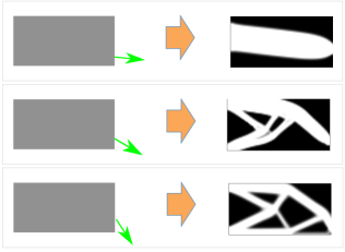
Figure 2: STO design space. Left: The loading on the right edge is parameterized by a vertical position, $p$, and a loading angle, $\theta$, and the filter size, $\rho$, which controls the length scale in the topology optimization. Right: Some of the more obvious connections between the force angle parameter choice, $\theta$ and resulting STO designs. A shallow angle of force encourages the material to be centrally located into what we refer to as a beam or beam-like structure (right-top). As the angle changes to become more inclined, the resulting design to includes smaller and smaller connections, ultimately becoming lattice-like because the collection of smaller beams form a kind of lattice (right-middle,-bottom).

Our experiments and evaluations will use solutions from the design of a cantilever beam that is clamped on the left edge and is under a static load on the right edge. The variable loading is parameterized by the vertical loading position, $p$, and the angle ($\theta$) of loading direction. The STO is further constrained by a filter size parameter, $\rho$, which determines the granularity of the material placements and effectively controls the size of the structures that are allowed to form in the solution. This design space is summarized on the left side of Figure 2.

Some specific design results are shown in the right side of Figure 2. In order to facilitate discussion, we will introduce some colloquial terminology we will use throughout the paper to describe various aspects of designs in this space. We will refer to designs which include a primary structure as a beam or beam-like, similar to the example on the top of Figure 2, and we will refer to examples with a collection of smaller connecting structures as a lattice or lattice-like, with one example shown on the bottom of Figure 2. Along those lines the design in the middle of Figure 2 we will describe as having both lattice-like features with a beam structure along the top side of the design. Additional examples can be found in a later part of the paper in Figure 4, as well as in many of the visualizations throughout.

3 Related work

3.1 Dimension reduction

The proposed method falls in the general class of dimensionality reduction (DR) techniques, but is designed to address specific challenges of feature summarization and coverage in the topology optimization context. However, because it shares many characteristics with more general DR we review that related work first to identify specific differences and similarities to existing methods.

An important aspect of our approach is to use examples from the dataset to summarize and represent the rest of the data. The idea of using a subset for DR is important and has been explored in other forms [12, 13, 14, 15, 16, 17]. In [17] they use examples to define the extents of an embedding space because the examples provide an undiluted representation of the underlying set. In another set of examples, [18] and [12] both use a subset of the dataset to represent the contents of data clusters or to identify points in a 2D embedded layout, because the subset presents a natural summary of data without any confusing abstraction or obfuscation. The works [13, 14, 15, 16] all use subsets because of their numerical closeness to the remaining data elements, allowing for the creation of powerful embedding methods. Subsets are a powerful representations because they contain details of the dataset, they avoid abstraction, and when selected appropriately can accurately represent neighbors.

One important goal of this work, which differentiates it from most DR approaches, is that we require a basis or axis after the DR transformation that easily relates back to the original data and provides explicit information on the existence of human-identifiable features (see Section 4.1 for a more precise treatment of this requirement). For the specific application to STO designs presented here, the axis should be easily related back to examples of STO designs, because these are physically meaningful and optimal, and become important for connecting designs and parameters. From the above discussion subsets are clearly an excellent choice to satisfy this interpretability constraint of STO summarization.

One of the most widely used DR techniques is principal component analysis (PCA) [19]. PCA seeks a linear projection to a lower dimension that maximally preserves variance of the dataset. While PCA is optimal in linear representation, the resulting basis is often quite difficult to interpret and frequently has only a vague relationship to the individual input data samples. In this paper we will examine PCA with respect to the STO application domain and show examples from an expert case study where using the PCA as the basis made otherwise simple tasks quite difficult. These same problems can also be found in many optimal basis or embedding techniques, such as independent component analysis (ICA) [20] and multidimensional scaling (MDS) [21, 22].

There are many nonlinear DR techniques, including nonlinear extensions of PCA, such as kernel PCA [23], or nonlinear geometric DR methods, such as Isomap [24] and local linear embedding (LLE) [25], that have been used to better model the geometric relationship of the data. While these approaches have arguably better representations of data on nonlinear manifolds, they do not directly address the interpretation problem, and, indeed, the resulting parameterizations often have no physical interpretation. Likewise, probabilistic nonlinear DR methods, such as stochastic neighbor embedding (SNE) [26], its t-distribution variant t-SNE [27], and parametric embedding (PE) [28], provide no clear interpretation relative to the original ensemble.

Improving DR from an interpretation standpoint has also been addressed in the literature [29, 30, 18]. While these methods aid in the use of standard DR techniques, they do not address the need for the axis to directly encode related human-identifiable features. For example, [29] and [30] both provide important tools for either finding the right point of view of the DR scatterplot or enhancing the choice of DR parameters for existing systems. Unfortunately, both cases, as with PCA, do not address the underlying problem that the DR axis obfuscate many of the human-identifiable features. [18] more closely addresses our needs by automatically selecting a subset to represent clusters in the DR. We compare to this general idea of clusters being representative of the data by using a k-medoids clustering for subset selection in some of our tests. The proposed approach is different in that it uses the subset, however it is determined, as the axis of the DR, while they perform a DR and then use a subset to represent resulting clusters. Additionally, the subset selection method from [18] has some fundamental problems which we directly address in our subset methodology. Their method first computes an singular value decomposition (SVD), closely related to PCA, and then finds points similar to the singular vectors (PCA modes). While this will work for specific datasets where points happen to lie near modes, this will not always be the case (this is similar to expecting the points to always lie near an average of the points). We instead propose selecting a subset that directly minimizes this representation error.

3.2 Subset-based visualization

The proposed work is strongly motivated by previous visualization research that has demonstrated the effectiveness of data subsets to understand the structure of a population. For instance, [14] uses greedy residual-based sampling to select the subset and PE, referred to above, to create two-dimensional embeddings.

Another set of related techniques is least square projection (LSP) [13] and part-linear multidimensional projection (PLMP) [15], that use a subset of the data to learn a linear low dimensional embedding. This is then applied to the full dataset. LSP is motivated by increasing the DR quality by limiting the learned projection to a set of control points, while PLMP is primarily motivated by computational challenges for extremely high dimensions datasets. LSP and PLMP both use clustering methods (k-medoids and bisecting k-means) to select the controls points. To understand the effectiveness of this, we evaluate k-medoids as a method for selecting a visualization subset and compare it to several other representation-motivated methods in this paper. Both LSP and PLMP result in a lower dimensional space whose axis are weighted combinations of the subset, similar to PCA.

Local affine multidimensional projection (LAMP) [16] provides for user selection of the subset and then uses that subset to produce a locally affine projection for the full dataset. Another interactive technique was presented in [17], where the user can interactively select basis extents from specific samples in the dataset, for the purposes of controlling how the scatter plot data is displayed. The proposed method differs from both in that the exemplars themselves are the axis and are selected automatically (rather than by the user), allowing it to scale to large subsets and large ensembles. Additionally, the proposed method automatically selects the subset based on some specific motivating criteria. Another point of difference is that [17] is focused entirely on a 2D scatter plot embedding, while we have used the proposed method almost entirely in higher-dimensional representations using alternative visualization strategies, such as parallel coordinates.

Design galleries [12] presents a 2D embedded layout and summarizes visual content of clusters or positions in the embedding using small multiples of a subset of the full dataset. This approach to using subsets for summarizing feature content of data points is quite effective, but is limited to 2D and 3D embeddings, which are often insufficient to adequately represent the high-dimensional data. This same limitation of embeddings also applies to many of the DR approaches described above. In the proposed approach, the dimensionality is only limited by the number of examples that can be shown in a row at the chosen screen and image resolutions.

3.3 Structural topology optimization analysis

Because we are not contributing directly to the methods of solving STO problems, we restrict our discussion to relevant work that analyzes or visualizes this type of data (for a more complete review of STO in general see, for example, [2]). In the domain of visualization, [3] introduced a complete system for finding and visualizing individual STO solutions. They present an impressive array of STO design spaces and visualization results, however their work focuses on the visualization of a single, complicated design space. Here, we are focused on understanding an ensemble of designs found by sampling different points in the parameter space or by different results from a stochastic process.

The work in [5] also has some overlap with this paper, because they use ensembles of designs to learn data driven models, relating the parameters to design solutions via a neural network. Their underlying motivation is to reduce the computational burden of finding new design solutions in the large design space. However, rather than learning a data driven relationship, we are instead interested in visualizing the data in such a way to allow the human designer to understand that relationship, and then apply that knowledge in future design problems. Additionally, [5] relies on PCA as the primary DR stage of their pipeline. This makes sense for a purely data-driven approach which does not address interpretability, and therefore has the previously described limitations.

4 Subset-based visualization of topology optimization designs

We propose a technique for visualizing a large collection of high-dimensional designs by first selecting a representative subset, using that subset as the visual basis, encoding the remaining data as linear combinations of those elements, and then displaying the resulting subset and encodings in standard visualization tools such as parallel coordinates [31] (or star coordinates [32, 33], scatter plot matrices [34], etc.).

An example is shown in Figure 3, where we have highlighted the main components of the subset-based visualization. The two main components are the subset display at the bottom (marked (B)), and the parallel coordinate plot of the weights relating the other data points to that subset (marked (A)). Because these are the main components of the visualization, careful selection of the type of subset and the properties of the weight relationship becomes very important. We additionally highlight a single coordinate axis in (C), with line positions along the axis correspond to reconstruction weights of all points using that element.

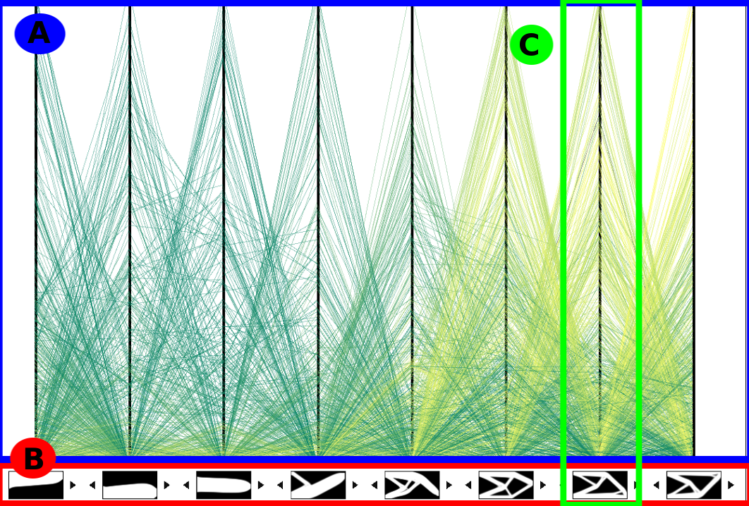
Figure 3: Diagram of the components of the proposed subset-based visualization using parallel coordinates. Component (A) shows the main parallel coordinate display that plots the computed weights of all data points on the chosen subset, by selecting and filtering this view, one gains an idea of what portion of the population is similar to the coordinate bases. Component (B) shows the subset axis figures. This subset represents the visual features of the dataset, and viewing the weights of the remaining points provides some intuitive idea of what each of the individual shapes consists of by considering the larger weights. Component (C) highlights a single coordinate axis, where the line positions along this axis are the weights of all points related to the highlighted subsample element.

4.1 Representative subset

The subset selection method can be motivated by different goals. For example, if we believe that data naturally stratifies into groups, a cluster-center-based subsample might be appropriate. In contrast, a random set of samples represents an unbiased subset. Because the typical screen size limits the number of basis elements that can be displayed (see Figure 3) it becomes critical to choose a subset that is both relatively small and that accurately represents the entire set of input data. For this reason, we formulate the representation goals of the subset decision precisely and then pursue optimum satisfaction of these goals. We define a subset as representative if linear combinations of that subset minimize the reconstruction error of the rest of the dataset.

If we express the input data in matrix form, $\mathbf{X}\in\mathbb{R}^{d\times n}$, where each column $\mathbf{x}_{i}\in\mathbb{R}^{d}$ is a data point and each row is a feature or dimension, the subset-based representation can be formulated so that $\mathbf{X}\approx\mathbf{R}=\mathbf{D}\tilde{\mathbf{B}}$, where $\mathbf{R}\in\mathbb{R}^{d\times n}$ is the representation (or reconstruction), $\mathbf{D}\in\mathbb{R}^{d\times m}$ is a subset of the data, and $\tilde{\mathbf{B}}\in\mathbb{R}^{m\times n}$ is the coefficients (or weights) used to combine the subsets into the approximate reconstructions. To find the most representative subset would mean simply minimizing the difference between the representation $\mathbf{R}$ and the input data $\mathbf{X}$, or

$$\min_{\tilde{\mathbf{B}},\mathbf{D}\subset\mathbf{A}}E(\tilde{\mathbf{B}},\mathbf{D}),$$ (1)

where,

$$E(\tilde{\mathbf{B}},\mathbf{D}) = \sum_{i}\|\mathbf{x}_{i}-\mathbf{D}\tilde{\mathbf{b}}_{i}\|_{2}^{2}$$ (2)

$$= \|\mathbf{X}-\mathbf{D}\tilde{\mathbf{B}}\|_{F}^{2},$$ (3)

in which we have used $\mathbf{D}\subset\mathbf{A}$ to denote that $\mathbf{D}$ is a column subset of $\mathbf{A}$.

In considering our specific STO problem, we found that domain experts are reliant on certain visual elements of the resulting designs which we refer to as human-identifiable features, or just features. For STO designs these include, for example, the number of internal holes, the number of thick beam structures, thin beam structures, how latticed the design is, etc. Consider some of the designs shown in Figure 4 (bottom two rows). These features are particularly important when making connections between parameters and designs. This idea of human-identifiable features is more general than for just STO designs and can change, appropriate to the domain.

As an intuitive example, we might consider the set of human faces that have features such as hair length, presence of facial hair, a hat, earings, etc., as seen in the sketched human faces (from [35]) in Figure 4 (top). These facial features are groups of data values (pixels) that have a correlated behavior across multiple images. For instance, longer hair is seen as sets of values/pixels on either side of the head that have dark values. Being able to identify the subset with the most representative features reduces computationally to finding the subset whose features (groups of pixels) maximally correlates with the rest of the dataset, which matches well with our formulation above. In the estimation and machine learning literature, research have observed that non-negative matrix factorization (NMF) has the property of extracting coherent features [36], by insisting that feature-capturing basis elements approximate the data by combining in a constructive manner. In other words, the non-negative constraint on weights tends to discourage the representation of data features through a negative-positive combination of large numbers of basis elements (as with PCA) and requires features (correlated values) to be represented explicitly in the basis elements. This effect can be seen in well-known negative-positive weighted decompositions such as Eigenfaces [37], which have face-like shapes but are difficult to interpret as clear facial features. Additionally, we will describe in our expert case study in Section 5.2.4, experiences where non-negative weights were easier for the participant to process mentally in terms of interpreting the combination of examples from the subset, reinforcing the importance of a non-negative weighting for relevant tasks.

With these details in mind, we further refine our goal in finding a representative subset which captures the most representative features by constraining the reconstruction weights, $\tilde{\mathbf{B}}$, to be non-negative. Thus, the non-negative formulation of the subset problem is:

$$\min_{\tilde{\mathbf{B}}\geq 0,\mathbf{D}\subset\mathbf{A}}E(\tilde{\mathbf{B}},\mathbf{D}).$$ (4)

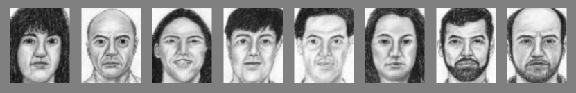
Figure 4: Representative subsets from face-sketch, STO D1, and STO D2. Top: representative subset from a face-sketch dataset [35], Middle: from the STO D1 design dataset with varying parameters and constant initialization, Bottom: from the STO D2 design dataset with constant parameters and varying initializations.

4.2 Simultaneous subset and coefficient computation

We now propose an approach for solving the optimization problem presented in the previous section. We can rewrite the objection function as,

$$E(\tilde{\mathbf{B}},\mathbf{D}) = \|\mathbf{X}-\mathbf{D}\tilde{\mathbf{B}}\|_{F}^{2}$$ (5)

$$= \|\mathbf{X}-\mathbf{X}\mathbf{B}\|_{F}^{2}=\hat{E}(\mathbf{B},m),$$ (6)

where $\mathbf{B}\in\mathbb{R}^{n\times n},\mathbf{b}_{i,:}=\tilde{\mathbf{b}}_{j,:}$, and $\tilde{\mathbf{b}}_{j,:}$ is the $j$-th row corresponding to the $j$-th data element in $\mathbf{D}$, the same as the $i$-th data element in $\mathbf{X}$. The smaller matrix $\tilde{\mathbf{B}}$ can be thought of as a submatrix of the larger more sparse $\mathbf{B}$, where $m$ specific (nonzero) rows are preserved.

Instead of building $\mathbf{B}$ from $\tilde{\mathbf{B}}$, we are interested in solving for $\mathbf{B}$ directly (and therefore obtain the embedded $\tilde{\mathbf{B}}$). The absolute optimum of the objective $\|\mathbf{X}-\mathbf{X}\mathbf{B}\|_{F}^{2}$ would result in $\mathbf{B}=\mathbf{I}$. However, if we constrain or regularize $\mathbf{B}$ so that it is row-sparse and non-negative, as described above, we can recover an optimal $\mathbf{B}$ with the desired properties. The regularization approach leads to this formulation for subset selection,

$$\mathbf{B}^{*}=\arg\min_{\mathbf{B}\geq 0}\|\mathbf{X-XB}\|_{F}^{2}+\lambda\|\mathbf{B}\|_{2,1}$$ (7)

where $\|\mathbf{B}\|_{2,1}=\sum_{i}\|\mathbf{B}_{:,i}\|_{2}$ is a mixed $\ell_{2,1}$ norm that induces row sparsity, where only a subset of the rows has nonzero entries, and $\mathbf{B}\geq 0$ means element-wise non-negativity ($b_{i,j}\geq 0,\forall i,j$).

The resulting $\mathbf{B}$ matrix encodes both the subset selection (corresponding to nonzero rows), and the weights connecting the rest of the dataset to the chosen subset (the values of the matrix). This is a convenient result as both the subset selection and weight computation occur simultaneously. This problem is known as a grouped lasso problem, and many solvers exist for efficiently estimating the matrix $\mathbf{B}$ [38, 39, 40]. We have found the method choice does not affect the resulting subset significantly, and have settled on using the fast grouped orthogonal matching pursuit (GOMP) solver[41], which was used in all results presented in this work.

4.3 Subset size

One important parameter to consider is the size of the subset. This parameter presents an important tradeoff. A larger subset will provide the opportunity to represent more unique features in the dataset, but a large enough subset could become cluttered, redundant, or even confusing. However, we have found that the screen space required for the proposed layout in Figure 3 is ultimately the limiting factor in the subset size, and so our recommendation is to use as many as the screen layout will allow, within reason. Another factor, which we have found useful in the decision, is to measure reconstruction error. For some datasets viewing the reconstruction error as a function of subset size can be helpful in determining a good tradeoff. In all of the experiments here, we use a subset of size 8, because we found this was appropriate for the screen displays used in our experiments and found it sufficiently large to capture the most important variations in the dataset.

4.4 Visual encoding

The method above places each design as a coordinate point in a medium-dimensional (e.g., $d=8$) space that is optimized to be representative and capture significant features. We have investigated a variety of methods for visually encoding the resulting representative subset coordinates, including scatter plot matrices, parallel coordinates, and star coordinates. Because of the non-negative combinations, the star-coordinate plot was promising. However, the documented ambiguities in the star-coordinate visualizations prevented sound exploration of the data and pattern discovery [34, 42]. The scatter plot matrix was difficult to use because of the large number of zero coefficients in the non-negative case, resulting in individual scatter plots that had points mainly clustered near the origin—the properties of which are unclear, but an area of ongoing consideration/investigation. Consequently, for this work we found the parallel coordinate visualization of the subset coordinates to be more effective, because it makes more visually apparent the coefficient relationships, better disambiguates data points, and, with the addition of interactive selection and filtering, makes it easier to find important relationships among data points. These motivations combined result in the proposed visualization shown in Figure 3.

4.5 Linked views

As described previously, the topology optimization designs are useful for STO task only when visualized coincident with parameters that gave rise to each design and corresponding scores related to expected functionality (e.g., maximum stress). Therefore, we augment the subset-based parallel coordinates view with a scatter plot showing combinations of the various parameters and scores. This additional view is then linked to the parallel coordinates view by using the same coloring, point selection, and filtering effects in both views.

We include two types of linked scatter plots. The first is a detailed view of the two selected axes from the parallel plots that we call the exemplar scatter plot. The second is a scatter plot that can use several options chosen by the user, from a t-SNE or isomap embedding of the dataset, to a scatter plot of specific parameters (angle, position, filter size) or score values (max stress, average stress, compliance). This additional visualization is a traditional scatter plot of parameter data, augmenting the subset display, and therefore the concerns about traditional DR techniques are not directly relevant. For example, some DR methods make cluster identification simple, and connecting that view to the proposed subset-based view would allow for fast interrogation of cluster attributes by visualization of the subset representations.

Additionally, we include a linked detail view that allows the user to view a specific data point and related details such as weight values. Figure 5 shows a few samples of each of these linked views, and Figure 1 shows a sample of them combined as a single visualization tool.

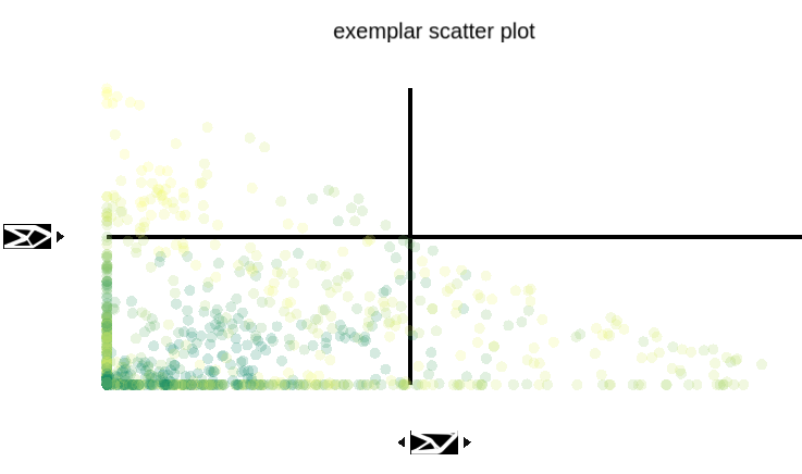
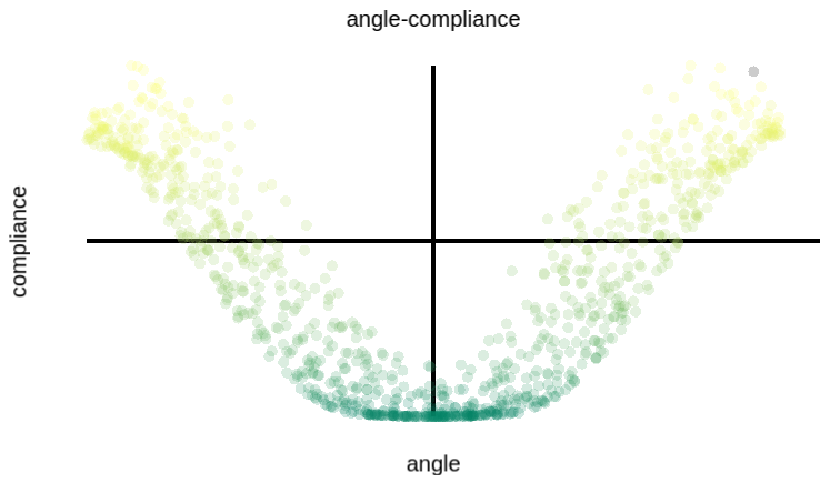
A           Exemplar scatter plot Parameter scatter plot           A

Example of the detail view showing a specific design
The colormap used throughout the examples

Figure 5: Linked scatter plot and detail view. Top: The exemplar scatter plot allowing detail view of two parallel coordinate views, and the second scatter plot view that can be set to a scatter plot of parameters (shown) or an embedding like t-SNE, Isomap, etc. as needed. Middle: An example of the detail view of a single data point including specific parameter values and weights used in a linear reconstruction. Bottom: The colormap used in all examples, representing low to high values of the user-selected parameter. For this figure points are colored according to average stress of the corresponding design.

5 Evaluation

We assessed the method in two parts. The first part, subset selection evaluation, focuses on evaluating the proposed subset selection method, using a quantitative analysis of feature coverage for each subset selection approach considered, and a quantitative assessment of representation error in a combined subset and weight computation. The second part, full system evaluation, focuses on the overall visualization with a quantitative analysis of successful task completion for the domain experts and a qualitative assessment of usage from a set of domain expert case studies. In addition to the evaluation, we include a final clarifying example to show how the full systems works on even very challenging datasets.

5.1 Subset selection evaluation

An important characteristic of the resulting subset is including examples of a broad range of user observable features of the dataset elements. The importance of this feature coverage arises from the need to represent a variety of points outside the chosen subset that will each include a potentially different mixture of those features. Likewise, any features not represented in the subset by definition will not be available in the visualization.

We consider our approach to compare feature coverage as a novel contribution, as we are unaware of previous work that has used feature coverage tests in this way to evaluate subset selection. This approach to measuring the level of coverage of the observable features allows a more direct, objective view of how well the subset represents what a user would see had they looked at all the elements of the dataset one by one.

The novelty is most easily seen in image-based datasets where observable features are difficult to extract automatically from the data elements. Specifically we select the subset using only the data elements, ignoring any manually-generated labels that would not be available in a completely new, unlabeled dataset that we would want to process. After selecting the subset, we use human-labeled visual features to determine quantitatively how well the subset covers the observable features – if the subset has a high coverage percentage, then it represents the dataset well, and if it has a low coverage percentage, then it does not represent the full dataset well. This comparison approach provides a strong indication of the quality of the subset from the point of view of representing the observable features in the full dataset.

5.1.1 Methods

We compared the proposed subset selection method, solved using non-negative group orthogonal matching pursuit (GOMP-NN), with the deterministic form of interpretable decomposition subset method (ID) [43, 44], the k-medoids method (KM) [45], and uniformly random subsets (RAND). The formulation of the proposed GOMP-NN approach was described previously in Section 4.2. ID is an appropriate alternative because it also simultaneously computes the weights, but it instead uses a pivoted-QR-type [44] subset selection, computing both positive and negative weights. KM (and related k-means) is a very well-known approach to clustering and/or quantizing a set of data, which also identifies cluster centers. Because KM does not explicitly prescribe a weight computation, we will look at both non-negative (KM-NN) and positive-negative weight options (KM-PN). RAND is a common method to subsample a dataset in an unbiased way. RAND also does not prescribe a specific type of weighting, so we compare against both options (RAND-NN and RAND-PN). One critical difference between GOMP-NN and either KM-NN or RAND-NN is that the non-negativity also drives the subset selection in GOMP-NN. In contrast, for KM-NN or RAND-NN, the nonnegative weights can only be computed after the subset selection.

In terms of asymptotic runtime, for a dataset with $n$ elements of $d$ dimension, GOMP is $\mathcal{O}(mn^{2}d)$, ID is $\mathcal{O}(mnd)$, KM is $\mathcal{O}(mndt)$, and RAND is $\mathcal{O}(1)$, where $t$ is the number of iterations to convergence for KM. For datasets where $n$ is the largest dimension, GOMP is the most expensive, followed by KM, and then ID. RAND is the fastest with a constant cost. However, the STO design datasets have a data dimension much larger than the number of points ($d>n$). Because of the high cost of solving for a single design, this situation will be common for general STO design ensembles. As the dimension of the design space increases, the cost for each solution will also increase, limiting the number of samples that can be solved. This indicates that asymptotic cost in $n$ will become less of an issue as larger systems are solved. From this vantage point, the runtime differences between GOMP, ID, and KM become less pronounced. KM is the only non-greedy method in terms of subset selection. For example, choosing $m$ verses $m+1$ subset elements can result in two different subset choices, while for both GOMP and ID the $m+1$ subset is the same as the $m$ subset except for the additional subset element found in the latest round. This is important when evaluating different size subsets because as the subset grows ID and GOMP both only require an additional sample to be found, where for KM the entire subset must be recomputed. Overall, for the STO design datasets we have not found a significant difference in runtime cost among methods (excepting RAND), and so limit the runtime discussion to this summary.

5.1.2 Datasets

We include an evaluation of subset method results on two datasets. One, CelebA, is a database of celebrity face images used in [46]. This dataset is of interest for the current problem because of the intuitive nature of the dataset type (everyone understands common face features). Also, this specific dataset contains a set of $40$ human-derived facial features amenable to the comparison, such as “mustache”, “eye glasses”, or “pointy nose”, etc. Evaluating this dataset also supports the claim that the proposed technique is more general than only STO design datasets. The original dataset consists of $2\times 10^{5}$ color face images of size $178\times 218$. Because this dataset is not the primary focus of the paper, we subsampled it both spatially (down sample by $4$) and randomly in the number of images (to $2\times 10^{4}$). As the STO datasets are much smaller than this down-sampled version, we consider this compromise acceptable.

The other, STO D1, is an STO design dataset, generated by collaborators/coauthors, with a design space of $40\times 80$ pixels and $10^{3}$ samples, where the structure of interest is attached to the left edge of the domain, and a point force is applied at some position $p\in[-20,20]$ and angle $\theta\in[0,\pi]$ on the right edge. The optimization is further constrained by a filter size $\rho\in[1.1,2.5]$ that controls how thin/thick structures are allowed in the solution (see Figure 2). A Monte Carlo sampling among these three parameters was used ($10^{3}$ samples), with the same constant initialization. Because this dataset did not have a predefined set of human-defined features like CelebA, we generated and evaluated them within a small-scale user study. A sample of the dataset is shown in the middle portion of Figure 4.

5.1.3 User-based evaluation of STO designs

To generate the human-defined features, we recruited one STO expert and eight different nonexpert graduate students. We asked the STO expert to specify a set of physically relevant features to describe the set of designs in a way that a nonexpert could understand, including things such as number of internal holes, number of external holes, thickness of the components, etc. We then asked three of the nonexpert participants to generate a set of visual features from their own assessment of the dataset. The expert and nonexperts each generated the feature set while being shown five random subsets of size 25 (125 total samples) from the dataset. One of the resulting nonexpert lists was not a binary feature set (as per the instructions) that had to be thrown out. After verifying both of the other nonexpert lists were binary feature sets (they could be evaluated in an approximate “yes” or “no” answer for any example), we randomly chose one of the remaining two nonexpert study for the remainder of the study, so that comparison could be made across participants.

We then asked five of the nonexperts to assess which of the subsets contained at least one instance of each feature in the expert list, and four do the same assessment but with the nonexpert list. Each nonexpert was completely blind to which subset they were assessing and the subsets were shown in a different order to each person. The assessed subsets were generated by GOMP-NN, ID, KM, and five different from RAND, resulting in eight total subsets being assessed by each participant for each list.

To compare two subsets we simply count how many features from each list were present in the subset – a subset which captures more of the features will better represent the remaining elements of the dataset.

5.1.4 Evaluation

We evaluate representation of each subset by reconstruction error and human-defined feature set coverage (count).

CelebA faces dataset. In terms of reconstruction error using non-negative weights for the subset sizes evaluated, GOMP-NN was always shown to be more representative than RANDOM-NN and KM-NN, while KM-NN did better than random for some subset sizes. For positive-negative weights, ID-PN and KM-PN did better than random for many sizes, but not all. Better here means the scores was better than the mean plus one standard deviation of the corresponding RANDOM. These quantitative representation results are shown in top of Figure 6.

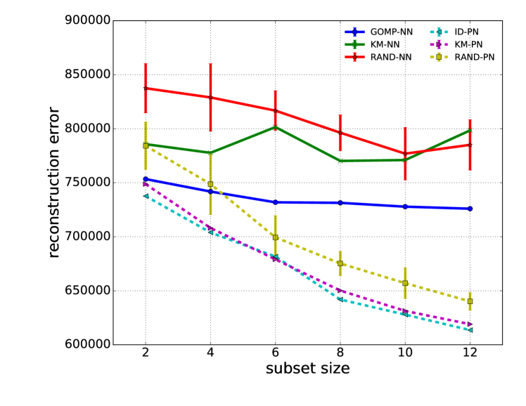
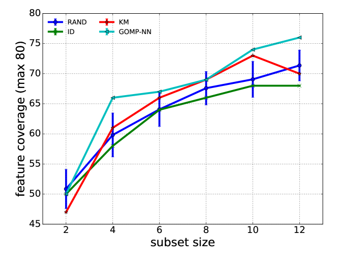
Figure 6: CelebA reconstruction error and coverage tests. Top: The reconstruction error for each subset type of size 2-12. Those using non-negative (NN) weights are shown with a solid plot line; positive-negative (PN) weighted reconstructions are shown with a dashed plot line. Bottom: The feature count found (out of 80) in each subset type. The random mean and standard deviation shown were computed over $10$ and $10^{2}$ samples respectively per measure.

However, the our comparison should also have some basis in how humans interpret the data. To establish this connection, we also consider the human-defined feature comparison. The results showed that GOMP-NN did better than random for all but two subset sizes, while among the others only KM really did better than random once, as shown in Figure 6. Note that different algorithms chose very different faces to get a similar number of features.

Topology optimization designs. The above human-face analysis showed that the proposed approach finds a representative subset in both the reconstruction error and the more qualitative human-defined-feature sense. For the specific case of STO designs, we performed a similar comparison. However, as described in Section 5.1.3, we created the feature list and feature assessment through a user-based evaluation strategy. This limited our evaluation to a single subset size, which we chose to be $8$ because that was the maximum number of subsamples we could show on the screen without the subsample resolution becoming too low in our visual layout. We will now summarize three types of results, a projection error comparison, an expert-feature-list-based assessment, and a nonexpert-feature-list-based assessment.

In the projection-error-based assessment we found that GOMP-NN was the most representative of the NN methods, while KM-PN was the most representative of the PN methods. In both cases all methods compared were more representative than the average random subset error. These results are summarized in Table I.

TABLE I: Shape reconstruction error test results for STO D1. The reconstruction error for each subset type of size 8. Those using non-negative (NN) weights are shown in the top part, positive-negative (PN) weighted reconstructions are shown in the lower part. The random mean and standard deviation were computed over $10^{2}$ samples. The lowest reconstruction error for each group is in bold font.

Method	Reconstruction error	Better?
GOMP-NN	628.51	Y
KM-NN	850.44	Y
RAND-NN	893.55(35.39)	N/A
ID	585.46	Y
KM-PN	537.59	Y
RAND-PN	609.33(26.52)	N/A

We also performed a similar comparison for a qualitative comparison of human-derived features. Rather than tag these features in all the designs, we had the participants assess the number of features present in each subset directly. This was a more reasonable amount of work for the number of participants we had, but it meant we were limited in the number of random subsets we could evaluate.

Even with the limited samples, we were able to show that for the expert feature list four of the five participants found that at least one of the nonrandom methods did better than random. Three of the five showed that both GOMP-NN and ID were better than RAND, while only one of the five showed KM-NN was better than RAND. Overall we interpret these results, summarized in Table II, as support for the methods specifically designed to select a representative set.

TABLE II: Shape feature coverage test results using expert list for STO D1. The feature count found (out of 45) from the expert feature list for each subset type of size 8, and whether this is better or not than random. Here, better means more than mean plus one standard deviation. The random mean and standard deviation were computed over five samples given to the same participant. The highest feature count for each participant is in bold font.

User	1	2	3	4	5
GOMP-NN	30	23	27	17	25
KM-NN	30	23	23	17	23
ID	31	26	26	17	24
RAND	27.0(4.1)	23.6(2.3)	24.6(1.9)	14.4(2.5)	21.8(1.6)
GOMP ?	N	N	Y	Y	Y
KM ?	N	N	N	Y	N
ID ?	N	Y	N	Y	Y
Any ?	N	Y	Y	Y	Y

For the nonexpert feature list we showed three out of four participants found an optimal method performed better than RAND. Specifically three out of four for GOMP-NN, two out of four for ID, and one out of four for KM-NN. While these results make little distinction among the type of subset methods, overall we take away that a method specifically designed to find a representative subset does in fact do better than RAND at feature representation. These results are summarized in Table III.

TABLE III: Shape feature coverage test results using nonexpert list for STO D1. The feature count found (out of 17) from the nonexpert feature list for each subset type of size 8, and whether this is better or not than random. The random mean and standard deviation were computed over $5$ samples given to the same participant. The highest feature count for each participant is in bold font.

User	1	2	3	4
GOMP-NN	11	14	13	15
KM-NN	12	12	7	13
ID	12	13	11	15
RAND	11.2(0.8)	12.4(1.5)	7.6(0.9)	11.0(1.0)
GOMP ?	N	Y	Y	Y
KM ?	N	N	N	Y
ID ?	N	N	Y	Y
Any ?	N	Y	Y	Y

5.2 Full system evaluation

Here we present an analysis of the full system from an STO domain expert point of view. For this analysis we had two domain experts (both coauthors) sit down and critically assess whether the tool successfully aids in building intuition around parameters, shapes, and quantitative design scores. While the domain experts are coauthors, we purposely had both play no role in the visualization development itself, limited mainly to helping the rest of the other authors understand what aspects of the data are important for them to explore and suggesting some visual interactions that could be helpful.

5.2.1 Methods

We use the same set of subset-selection and weight-computation methods explored in Section 5.1. However, because manual visual assessment is more limiting in time than the quantitative assessments done earlier, we limited the comparison among GOMP-NN, KM-NN, ID. Because prior work uses PCA to analyze these type of datasets, we also included a PCA version of the parallel coordinates view with the appropriate positive-negative weighting, referred to as PCA, shown in Figure 7. This provided four different axes and weighting choices, two with non-negative weighting and two with positive-negative weighting.

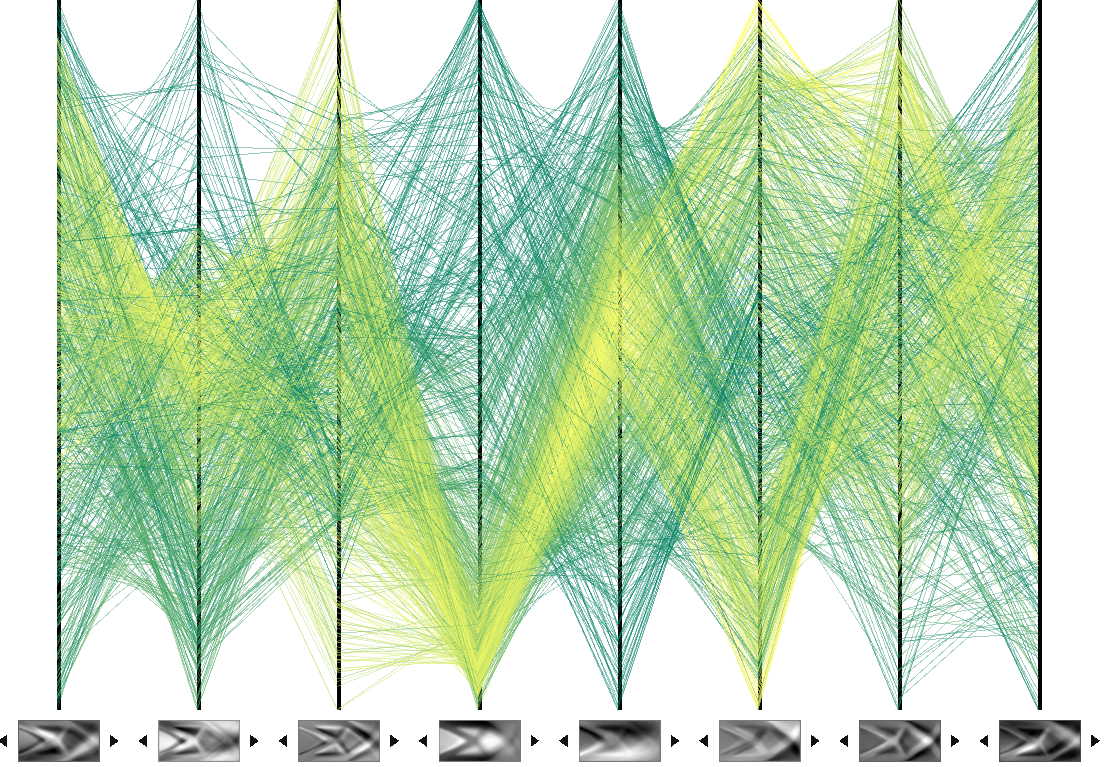
A           PCA as basis ID as basis           A

Figure 7: Alternatives non-negative weighted subset views. Left: The same visualization approach but using a PCA basis for the axis. Users found this approach very confusing both for the axes representation and attempting to combine them mentally using positive and negative weights. Right: Subset-based visualization using ID with its positive-negative weights. Users also found this combination confusing because it was difficult to manually subtract one image from another.

5.2.2 Datasets

The same parameter varying STO design dataset, STO D1 (described in Section 5.1.2), was used for this qualitative study. We also included a second STO design dataset, STO D2, where the three parameters were fixed to $p=0$, $\theta=\pi/4$, and $\rho=1.1$ respectively, but the initial configuration was initialized randomly, resulting in $1000$ different designs. Because of the nonconvex nature of the STO problem, the resulting ensemble had a large variety of latticed designs, although total design variance was not as great as STO D1. The domain experts also had much less initial intuition about this dataset. A sample from both datasets is shown in Figure 4.

5.2.3 Evaluation

Before viewing the final visualization tool, we asked the two domain experts to report any relationships they were already aware of between parameters, designs, and scores. We then translated those into a set of tasks: confirm each relationship known beforehand. The number of these prior known relationships that can be confirmed by each version of the tool is used as a quantitative measure for comparison. During the case studies, the experts were unaware of which type of subset-weight combination was shown (labeled A,B,C), except for PCA because of the obvious nature of the axes figures. In addition to evaluating how many prior relationships were confirmed, we also asked the experts to explore the data with the tool and report any additional relationships or other insights they gained during the use that we report as well.

Task completion assessment. Most of the relationships the domain experts were aware of before the visualization focus session involved simple parameter-to-shape relationships, such as position and contact point, angle and structure composition (lattice vs beam), and filter size and beam thickness. There was one relationship between shape and scoring: having many holes should lead to high stress values. Finally, one relationship among scores, specifically that stress and compliance should correlate well. One detail to note is that there was almost no prior intuition about the second dataset with fixed parameters and random initializations. We summarize the relationships identified before using the visualization technique along with specific numbers for easy reference in Table IV (top portion).

While exploring the datasets the experts arrived at several unknown, or at least unstated, relationships between the parameters and scores, such as position and compliance, angle and compliance. They also confirmed some unstated assumptions, such as all designs are variations among purely beam and purely lattice designs. The experts were also able to gain some intuition about the various shapes that arose in the second dataset. Specific relationships found in the study are shown in the lower portion of Table IV with a number and asterisk to distinguish them from the first group.

After allowing for exploration, we tasked the experts to confirm each of the relationships they identified before using the tool. Using the complete tool, the experts were able to confirm all prior relationships quite quickly with any of the basis types.

Because of the multiple components in the visualization we next tried to understand at a finer granularity how each piece aided in the confirmation process by removing some components. One particular modification that revealed a more informative comparison was to remove the detail plot entirely, so that the expert had to rely entirely on the parallel coordinate plot to both summarize the dataset designs and to tease out specific details of the designs and how they relate to the parameters and scores. This change resulted in different performance among the methods.

Specifically, the experts found it very difficult to confirm all but one of the known relationships using the PCA basis or the ID basis. When asked why it was difficult, they were quite critical of the PCA basis set and weights, as it was “impossible to combine the bases, especially with the positive-negative weights”. In essence, the experts found it very difficult to mentally combine the PCA basis to understand any of the reconstructions. One particularly illuminating example is that none of the PCA bases showed an example of a beam, because all beam representations were recreated by subtracting lattice-looking bases from each other; an example is shown in Figure 8. The ID subset visualization was also difficult for the experts to use in confirming relationships. Even though the axes were a subset of the designs, the positive-negative weights made the mental combination of examples difficult. This confirms our hypothesis, which is that constructive combinations of features allows for easier interpretation of data represented as mixtures of basis elements.

Example of beam reconstruction using PCA

Example of beam reconstruction using a subset

Figure 8: Beam reconstruction using PCA compared to a subset reconstruction. Top: Shows a straight beam design and how it is represented using PCA modes. Note that none of the basis elements looks like a beam, but by combining them in positive and negative fashion the original beam can be reconstructed quite accurately. Bottom: The same straight beam represented by a subset. Because some of the basis elements (subset elements) do look like a beam it is quite easy to mentally reconstruct what the data element would look like, if you did not have the design itself to view (perhaps due to space). Note that a similar problem would occur with subset visualization if the subset did not contain a beam structure, which is another motivation for using the proposed subset selection technique by definition it is the optimal subset for reconstruction using non-negative weights.

In contrast, the experts were able to confirm most of the prior relationships using KM-NN and GOMP bases. Consider the example comparison in Figure 8 where mentally extracting a beam design from the PCA basis is quite difficult, in contrast to the very obvious beam structure indicated by the subset visualization example. For some of the relationships, experts claimed a partial confirmation because of a desire to view more samples of some of the more detailed aspects of the dataset than those available. That experience outlines one limitation of the approach – that while the subset-based view provides a good overview of the dataset with feature details, it is difficult to extrapolate out to feature details not represented in the subset.

Most of this discussion has centered around the first of the two STO datasets, but results were also investigated for the second dataset. Most of the prior assumptions were not applicable to the second dataset because the parameters were fixed, but for the two that did apply we observed similar results. The precise results are summarized in Table V.

TABLE IV: Relationships reported by domain experts. The relationships reported before viewing the visualization tool are summarized in the top portion of table with assigned numbers. The relationships reported (discovered) while using the tool are reported in the lower half of the table (numbers with asterisks).

relationship	description
1	position and right side contact point
2	angle horizontal then structure horizontal
3	low angle and varying positions then shallow
	angle straight structure
4	filter size controls structure thickness
5	more holes in structure then higher stress
6	compliance and stress are correlated
7*	symmetric-quadratic relationship between
	position and compliance/stress
8*	position choice induces an upper limit
	on compliance (lowest at 0)
9*	negative correlation between angle and compliance
10*	all of the designs are variations of a beam or
	lattice design (confirmation)

TABLE V: Prior known relationships assessments by domain experts. Verification of known relationships described in Table IV using various versions of the visualization tool (by changing axis and visualization components). Detail indicates use of visualization with detail view, otherwise the detail view was excluded. Results are shown for the first (STO D1) and second (STO D2) datasets in upper and lower parts of the table, respectively. Here Yes (Y) means confirmed, No (N) cannot confirm, Partial (P) means confirmed but want more samples to be completely sure.

relationship	1	2	3	4	5	6
Detail (D1)	Y	Y	Y	Y	Y	Y
GOMP-NN (D1)	Y	P	Y	P	P	Y
ID (D1)	N	N	N	N	N	Y
KM-NN (D1)	P	P	P	N	P	Y
PCA (D1)	N	N	N	N	N	Y
Detail (D2)	-	-	-	-	Y	Y
GOMP-NN (D2)	-	-	-	-	P	Y
ID (D2)	-	-	-	-	N	Y
KM-NN (D2)	-	-	-	-	P	Y
PCA (D2)	-	-	-	-	N	Y

5.2.4 Case studies

We now present several case studies from the domain expert session. These case studies detail some of the uses we found for the tool, and identify some of the specific strengths and limitations of the proposed subset-based visualization.
Subset-based parallel coordinate view as surrogate to full dataset. As part of the relationship confirmation task above, we forced the domain experts to not use the detail view (individual elements), and the resulting use of the visualization was quite illuminating. When limited to the the subset-based parallel coordinate view, the experts selected points in the parameter scatter plot and then looked at which of the subset elements contained large weights. For the case of non-negative weighted views, they used those values to mentally consider what the element looks like and make a conclusion. This subset-based view usage is in contrast to the individual element view, where the experts selected points from the parameter scatter plot and looked at the corresponding element. To summarize, the subset-based view was being used as a surrogate for the full dataset in completing the confirmation tasks mentioned above. Note that in this same setting when the subset-based view was changed to use positive-negative weights or the PCA basis elements, this summarizing ability of the parallel coordinate view was apparently lost. In considering this aspect of the subset-based parallel coordinate view, the domain experts commented that it “Allows for a whole-view perspective of the data, instead of viewing the data elements individually”.
Limitations of subset-based view. One of the tasks was to confirm that the filter size influenced the size of the structures in the design (smaller filter size results in smaller lattice structures and other features). However because the subset contains only a limited number of the smaller lattice structure examples, the expert was unable to confirm the relationship fully, marking it as “partially” confirmed. Because the experts had previously confirmed the relationship using individual instances, they were expecting to see more examples of the relationship than what was available. The experience highlights one limitation of the method: when any feature is not included in the subset, the surrogate nature of the view is not nearly as true to the underlying dataset. This point emphasizes that the choice of subset becomes crucial to success, and why we advocate the use of the GOMP-NN-based selection.
Confirmation of design shape aspect of parameter-score relationships. The domain experts were able to discover new relationships among parameters and scores, for example relationships 7*,8*, and 9*, in Table IV. These relationships have implications for the design shapes themselves, and in each case the experts were able to use the subset-based view to understand that relationship. For example, for relationship 9* they were able to show that the steeper angle resulted in a more latticed structure that had more holes and higher stress values.
Exemplar scatter plot as summary device. The exemplar scatter plot, although not used extensively by the experts, did become useful for understanding and confirming general trends in the dataset, as well as for understanding the parallel coordinates plot at times. For example, the domain experts were able to confirm that the STO designs can be largely grouped into two large sets, those that have a large central beam, and those that are mainly lattice structure. This confirmation was accomplished by viewing the exemplar scatter plot with a beam structure on one axis, and a purely lattice structure on the other axis.
Parameter scatter plot as driver for discovery. For the full tool, the parameter-based scatter plots (i.e., scatter plot of angle and compliance) that is then colored by a third variable such as maximum stress, proved to be the primary tool used to drive discovery. The basic workflow consists of the experts looking at relationships on that plot, and then using the linked-nature of the views to explore visual aspects of the relationships in the subset-based visualization and the detail view.
Limitations of PCA- and ID-based views. The limitations of the PCA view became very evident in the domain expert study. While using the subset view, they were able to confirm and gauge general visual trends in the data, but when using the PCA version of the tool the users became quite frustrated. Some of the phrases used to describe their reaction are: “I can’t see any beams in the modes”, “convoluted examples… look like photo negatives… or ghosts of the structures”, and “the axis are no longer intuitive”. The positive-negative weights also played a role in the confusion. This was discovered by using the ID-based subset view, that uses subsets but with positive-negative weights. While the axes were easier to understand for the users, trying to mentally subtract examples from each other was difficult to do. When the bases were PCA modes, the task became even more difficult.

5.2.5 Additional examples

To further discuss some of the points made above, and to further demonstrate how the system benefits from the use of a subset-based display of the designs, we will now present some examples of the more challenging STO2 datasets. These example were not included in the case study, but are presented here for further illumination of the points brought up previously. Note that the STO2 dataset mentioned above, used as part of the expert case study, is more challenging to understand, even for an expert, because the only parameter that was changed was the initial material placement. In other words, the angle, position, and filter size parameters are all constant. This makes the dataset difficult to interpret because there is no longer a clear connection between parameter choice and the resulting STO design. However, we will show that the system is still quite useful for understanding the connection between attributes, such as stress, and the visual design.

The subset-based summary is shown in Figure 9 where the STO2 dataset has been loaded. The display is using the GOMP-NN basis and weights with a high stress example selected and highlighted in the left figure, and a low stress figure has been highlighted in the right figure. Because the subset-based view captures and shows the a subset of the dataset, which in this case appears to be the differing lattice structure, it becomes quite clear from the visualization that the more lattice structure there is in the design the higher the stress becomes.

A                            High stress example selected Low stress example selected                            A

Figure 9: GOMP-NN view of the more challenging STO2 dataset. This example shows how visual features can be directly connected to low and high stress using a subsample-based view (more lattice structure correlates with high stress).

Now contrast the very clear interpretation of that observation with what we see in the PCA-based view shown in Figure 10. Again we show the same high stress example in the left part of Figure 10 and the same low stress example in the right part. Now, because of the choice of PCA basis, it is quite difficult to understand what, if any, relationship can be seen using this view of the data.

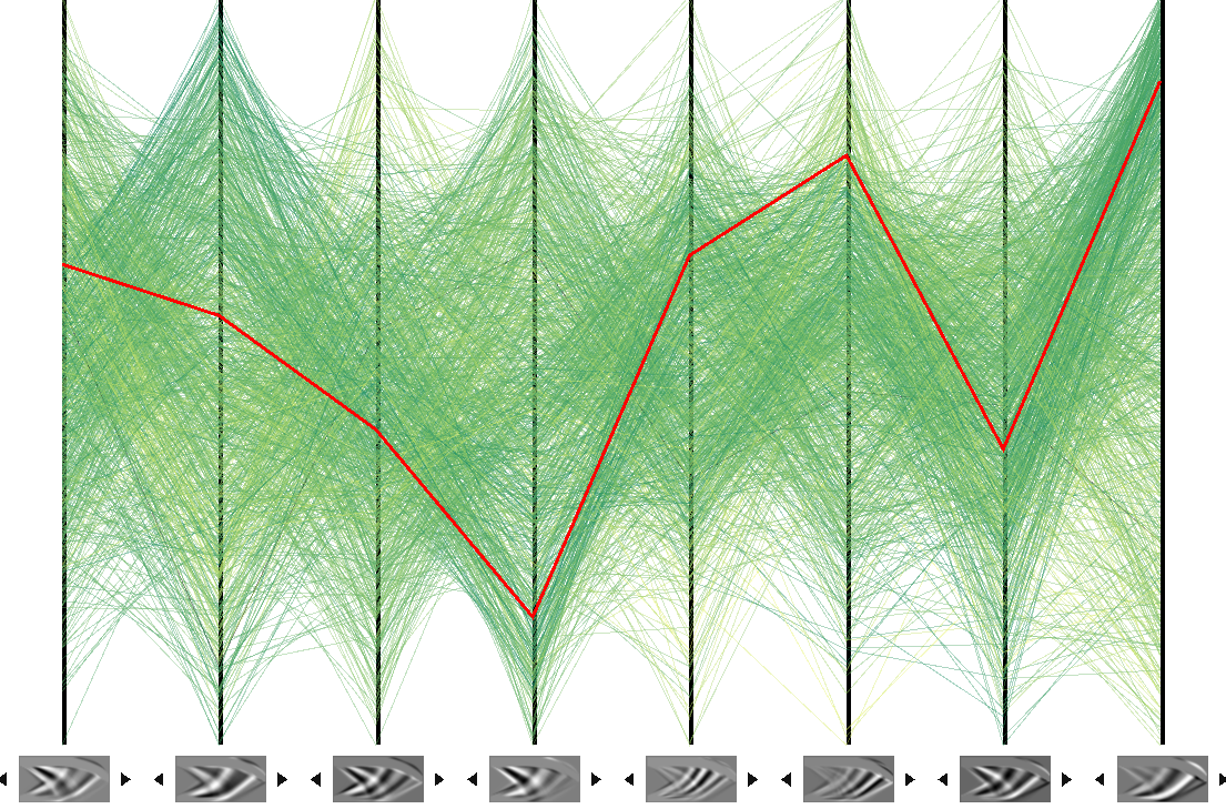
A                            High stress example selected Low stress example selected                            A

Figure 10: PCA view of the more challenging STO2 dataset. This example shows how it is difficult to find a connection between low and high stress and the design features using a PCA-based view.

This example reinforces what we observed on other datasets, such as STO1, CelebA, and the sketch face database. In terms of interpretability, a subset-based view provides superior summarization to PCA and related basis choices.

6 Discussion

Strengths. The representative subset view appears to be an appropriate technique for summarizing a dataset of visual features, and specifically for STO designs. By linking the subset-based view to the STO parameters through coloring and interactive selection, the visualization allows for a parameter-driven exploration of the dataset while the subset view provides the needed dataset visualization, avoiding the need to display all individual designs for most tasks. The method also appears suitable for more general datasets with visual features, and potentially non-visual features given appropriate linked views.

Limitations. Extrapolation of any features not present in subset is difficult to make, which can limit the amount of detailed relationships that can be found using the subset view. Additionally, our proposed method is limited to design spaces where linear combinations work. While we have found this to work for STO designs, some design spaces will require a different approach. In terms of our assessment, we limited ourselves (on purpose, for matters of scope) to 2D design spaces, but in the future it would be interesting to consider higher dimensional design spaces. While we explored several aspects of the method, our assessment was primarily based around the STO design dataset and the CelebA image database. In the future we would like to explore how this approach benefits in other data types, such as text and other nonspatial datasets.

Conclusions. The proposed visualization method has significant advantages over traditional dimension-reduction-based techniques in terms of allowing a domain expert to extrapolate and infer details of the dataset from a small, carefully chosen subset. For STO design this specifically allows connecting parameters and score values back to visual design features in many cases. The suggested optimally representative GOMP-NN-based subset selection has been shown to be the most representative in terms of reconstruction error for non-negative weighting and, in a more qualitative sense, more representative of human-determined features than a random dataset. Finally, expert case-studies have identified some of the strengths and limitations of the proposed approach.

References

- [1] M. P. Bendsøe and N. Kikuchi, “Generating optimal topologies in structural design using a homogenization method,” Computer methods in applied mechanics and engineering, vol. 71, no. 2, pp. 197–224, 1988.
- [2] M. P. Bendsoe and O. Sigmund, Topology Optimization: Theory, Methods, and Applications. Springer Science & Business Media, 2003.
- [3] J. Wu, C. Dick, and R. Westermann, “A system for high-resolution topology optimization,” IEEE transactions on visualization and computer graphics, vol. 22, no. 3, pp. 1195–1208, 2016.
- [4] U. Schramm and M. Zhou, “Recent developments in the commercial implementation of topology optimization,” in IUTAM symposium on topological design optimization of structures, machines and materials. Springer, 2006, pp. 239–248.
- [5] E. Ulu, R. Zhang, and L. B. Kara, “A data-driven investigation and estimation of optimal topologies under variable loading configurations,” Computer Methods in Biomechanics and Biomedical Engineering: Imaging & Visualization, vol. 4, no. 2, pp. 61–72, 2016.
- [6] A. Sutradhar, G. H. Paulino, M. J. Miller, and T. H. Nguyen, “Topological optimization for designing patient-specific large craniofacial segmental bone replacements,” Proceedings of the National Academy of Sciences, vol. 107, no. 30, pp. 13 222–13 227, 2010.
- [7] T. A. Reist, J. Andrysek, and W. L. Cleghorn, “Topology optimization of an injection moldable prosthetic knee joint,” Computer-Aided Design and Applications, vol. 7, no. 2, pp. 247–256, 2010.
- [8] J.-H. Zhu, W.-H. Zhang, and L. Xia, “Topology optimization in aircraft and aerospace structures design,” Archives of Computational Methods in Engineering, vol. 23, no. 4, pp. 595–622, 2016.
- [9] W. Chen, M. Fuge, and J. Chazan, “Design manifolds capture the intrinsic complexity and dimension of design spaces,” Journal of Mechanical Design, vol. 139, no. 5, p. 051102, 2017.
- [10] D. Brackett, I. Ashcroft, and R. Hague, “Topology optimization for additive manufacturing,” in Proceedings of the solid freeform fabrication symposium, Austin, TX, 2011, pp. 348–362.
- [11] B. S. Lazarov, F. Wang, and O. Sigmund, “Length scale and manufacturability in density-based topology optimization,” Archive of Applied Mechanics, vol. 86, no. 1-2, pp. 189–218, 2016.
- [12] J. Marks, B. Andalman, P. A. Beardsley, W. Freeman, S. Gibson, J. Hodgins, T. Kang, B. Mirtich, H. Pfister, W. Ruml et al., “Design galleries: A general approach to setting parameters for computer graphics and animation,” in Proceedings of the 24th annual conference on Computer graphics and interactive techniques. ACM Press/Addison-Wesley Publishing Co., 1997, pp. 389–400.
- [13] F. V. Paulovich, L. G. Nonato, R. Minghim, and H. Levkowitz, “Least square projection: A fast high-precision multidimensional projection technique and its application to document mapping,” IEEE Transactions on Visualization and Computer Graphics, vol. 14, no. 3, pp. 564–575, 2008.
- [14] Y. Chen, L. Wang, M. Dong, and J. Hua, “Exemplar-based visualization of large document corpus,” IEEE Transactions on Visualization and Computer Graphics, vol. 15, no. 6, 2009.
- [15] F. V. Paulovich, C. T. Silva, and L. G. Nonato, “Two-phase mapping for projecting massive data sets,” IEEE Transactions on Visualization and Computer Graphics, vol. 16, no. 6, pp. 1281–1290, 2010.
- [16] P. Joia, D. Coimbra, J. A. Cuminato, F. V. Paulovich, and L. G. Nonato, “Local affine multidimensional projection,” IEEE Transactions on Visualization and Computer Graphics, vol. 17, no. 12, pp. 2563–2571, 2011.
- [17] H. Kim, J. Choo, H. Park, and A. Endert, “Interaxis: Steering scatterplot axes via observation-level interaction,” IEEE transactions on visualization and computer graphics, vol. 22, no. 1, pp. 131–140, 2016.
- [18] P. Joia, F. Petronetto, and L. G. Nonato, “Uncovering representative groups in multidimensional projections,” in Computer Graphics Forum, vol. 34, no. 3. Wiley Online Library, 2015, pp. 281–290.
- [19] I. Jolliffe, Principal component analysis. Wiley Online Library, 2002.
- [20] A. Hyvärinen, J. Karhunen, and E. Oja, Independent component analysis. John Wiley & Sons, 2004, vol. 46.
- [21] J. B. Kruskal and M. Wish, Multidimensional scaling. Sage, 1978, vol. 11.
- [22] S. Ingram, T. Munzner, and M. Olano, “Glimmer: Multilevel mds on the gpu,” IEEE Transactions on Visualization and Computer Graphics, vol. 15, no. 2, pp. 249–261, 2009.
- [23] B. Schölkopf and A. J. Smola, Learning with kernels: support vector machines, regularization, optimization, and beyond. MIT press, 2002.
- [24] J. B. Tenenbaum, V. De Silva, and J. C. Langford, “A global geometric framework for nonlinear dimensionality reduction,” science, vol. 290, no. 5500, pp. 2319–2323, 2000.
- [25] S. T. Roweis and L. K. Saul, “Nonlinear dimensionality reduction by locally linear embedding,” Science, vol. 290, no. 5500, pp. 2323–2326, 2000.
- [26] G. E. Hinton and S. T. Roweis, “Stochastic neighbor embedding,” in Advances in neural information processing systems, 2002, pp. 833–840.
- [27] L. Van der Maaten and G. Hinton, “Visualizing data using t-sne,” Journal of Machine Learning Research, vol. 9, no. 2579-2605, p. 85, 2008.
- [28] T. Iwata, K. Saito, N. Ueda, S. Stromsten, T. D. Griffiths, and J. B. Tenenbaum, “Parametric embedding for class visualization,” Neural Computation, vol. 19, no. 9, pp. 2536–2556, 2007.
- [29] D. B. Coimbra, R. M. Martins, T. T. Neves, A. C. Telea, and F. V. Paulovich, “Explaining three-dimensional dimensionality reduction plots,” Information Visualization, vol. 15, no. 2, pp. 154–172, 2016.
- [30] R. M. Martins, D. B. Coimbra, R. Minghim, and A. C. Telea, “Visual analysis of dimensionality reduction quality for parameterized projections,” Computers & Graphics, vol. 41, pp. 26–42, 2014.
- [31] A. Inselberg and B. Dimsdale, “Parallel coordinates: a tool for visualizing multi-dimensional geometry,” in Proceedings of the 1st conference on Visualization’90. IEEE Computer Society Press, 1990, pp. 361–378.
- [32] E. Kandogan, “Star coordinates: A multi-dimensional visualization technique with uniform treatment of dimensions,” in Proceedings of the IEEE Information Visualization Symposium, vol. 650. Citeseer, 2000, p. 22.
- [33] ——, “Visualizing multi-dimensional clusters, trends, and outliers using star coordinates,” in Proceedings of the seventh ACM SIGKDD international conference on Knowledge discovery and data mining. ACM, 2001, pp. 107–116.
- [34] S. Liu, D. Maljovec, B. Wang, P. Bremer, and V. Pascucci, “Visualizing High-Dimensional Data : Advances in the Past Decade,” Eurographics Conference on Visualization (EuroVis), 2015.
- [35] X. Wang and X. Tang, “Face photo-sketch synthesis and recognition,” IEEE Transactions on Pattern Analysis and Machine Intelligence, vol. 31, no. 11, pp. 1955–1967, 2009.
- [36] D. D. Lee and H. S. Seung, “Learning the parts of objects by non-negative matrix factorization,” Nature, vol. 401, no. 6755, pp. 788–791, 1999.
- [37] M. A. Turk and A. P. Pentland, “Face recognition using eigenfaces,” in Computer Vision and Pattern Recognition, 1991. Proceedings CVPR’91., IEEE Computer Society Conference on. IEEE, 1991, pp. 586–591.
- [38] M. Yuan and Y. Lin, “Model selection and estimation in regression with grouped variables,” Journal of the Royal Statistical Society: Series B (Statistical Methodology), vol. 68, no. 1, pp. 49–67, 2006.
- [39] S. Boyd, “Alternating Direction Method of Multipliers,” Proceedings of the 51st IEEE Conference on Decision and Control, vol. 3, no. 1, pp. 1–44, 2011.
- [40] W. Deng, W. Yin, and Y. Zhang, “Group Sparse Optimization By Alternating Direction Method,” SPIE Optical Engineering + Applications, pp. 88 580R–88 580R, 2013. [Online]. Available: http://circ.ahajournals.org/cgi/content/abstract/95/2/473
- [41] J. Kim, R. Monteiro, and H. Park, “Group sparsity in nonnegative matrix factorization,” In proc. of the 2012 SIAM International Conference on Data Mining (SDM), pp. 851–862, 2012.
- [42] D. J. Lehmann and H. Theisel, “Orthographic star coordinates,” IEEE Transactions on Visualization and Computer Graphics, vol. 19, no. 12, pp. 2615–2624, 2013.
- [43] H. Cheng, Z. Gimbutas, P.-G. Martinsson, and V. Rokhlin, “On the compression of low rank matrices,” SIAM Journal on Scientific Computing, vol. 26, no. 4, pp. 1389–1404, 2005.
- [44] G. Golub, “Numerical methods for solving linear least squares problems,” Numerische Mathematik, vol. 7, no. 3, pp. 206–216, 1965.
- [45] H.-S. Park and C.-H. Jun, “A simple and fast algorithm for k-medoids clustering,” Expert systems with applications, vol. 36, no. 2, pp. 3336–3341, 2009.
- [46] Z. Liu, P. Luo, X. Wang, and X. Tang, “Deep learning face attributes in the wild,” in Proceedings of International Conference on Computer Vision (ICCV), 2015.