Nuclear spin squeezing by continuous quantum non-demolition measurement: a theoretical study

Abstract

We propose to take advantage of the very weak coupling of the ground-state helium-3 nuclear spin to its environment to produce very long-lived macroscopic quantum states, here nuclear spin squeezed states, in a gas cell at room temperature. To perform a quantum non-demolition measurement of a transverse component of the previously polarized collective nuclear spin, a discharge is temporarily switched on in the gas, which populates helium-3 metastable state. The collective spin corresponding to the $F=1/2$ metastable level then hybridizes slightly with the one in the ground state by metastability exchange collisions. To access the nuclear spin fluctuations, one continuously measures the light field leaking out of an optical cavity, where it has interacted dispersively with the metastable state collective spin. In a model of three coupled collective spins (nuclear, metastable and Stokes for light) in the Primakoff approximation, and for two measurement schemes, we calculate the moments of the collective nuclear spin squeezed component $I_{z}$ conditioned on the optical signal averaged over the observation time $t$. In the photon counting scheme, we find that the squeezed observable is $I_{z}^{2}$ rather than $I_{z}$. In the homodyne detection scheme, we analytically solve the stochastic equation for the state of the system conditioned on the measurement; the conditional expectation value of $I_{z}$ depends linearly on the signal and the conditional variance of $I_{z}$ does not depend on it. The conditional variance decreases as $(\Gamma_{\rm sq}t)^{-1}$, where the squeezing rate $\Gamma_{\rm sq}$, which we calculate explicitly, depends linearly on the light intensity in the cavity at weak atom-field coupling and saturates at strong coupling to the ground state metastability exchange effective rate, proportional to the metastable atom density. Finally, we take into account the de-excitation of metastable atoms at the walls, which induces nuclear spin decoherence with an effective rate $\gamma_{\alpha}$. It imposes a limit $\propto(\gamma_{\alpha}/\Gamma_{\rm sq})^{1/2}$ on the conditional variance reached in a time $\propto(\gamma_{\alpha}\Gamma_{\rm sq})^{-1/2}$. A multilingual version is available on the open archive HAL at https://hal.archives-ouvertes.fr/hal-03083577.
Keywords: spin squeezing ; helium 3 ; nuclear spin ; quantum metrology ; stochastic wave functions

1 Introduction

Helium-3 in its ground state enjoys the remarkable property of having a purely nuclear spin $1/2$, perfectly isolated from the outside world even in an environment as hostile to quantum coherences as a gas of helium in a centimetric cell at room temperature and a pressure of the order of a millibar. By well-mastered nuclear polarization techniques, reaching a polarization of 90 $\%$, we can then routinely prepare (for example for lung imaging by nuclear magnetic resonance MacFall1996 ) a giant collective nuclear spin with an extremely long lifetime. Recently, a coherence time $T_{2}$ larger than 60 hours was measured in ultra-precise magnetometry devices Heil2010 , that seems limited only by the longitudinal decay time $T_{1}$ due to collisions with the cell walls. These numbers make the macroscopic nuclear spin in a room temperature gas an ideal system for the production, the study and the use of entangled states, and therefore a competitor of cold atomic gases and Bose-Einstein condensates in metrology and quantum information processing PezzeRMP . Already in 2005, we suggested that the nuclear spins of helium-3 could give rise to quantum memories DantanReinaudi2005 or to non-local quantum states Reinaudi2007 with very long lifetimes. Since then, experimental breakthroughs have been made in the field of spin squeezing, notably by means of non-demolition quantum measurements (QND) in atomic alkali gases interacting with the electromagnetic field PezzeRMP ; stroboscopic ; Kasevich ; Xiao , which recently made it possible to obtain a squeezed spin state with a lifetime of one second in the hyperfine ground state of rubidium under metrological conditions Myles2020 . We recall that, in analogy with the squeezed states of light in quantum optics, a (here collective) spin $\vec{I}$ is said to be squeezed if it admits reduced fluctuations with respect to the standard quantum limit in a direction $z$ orthogonal to that $x$ of the mean spin ; this leads to increased accuracy in pointing the mean spin in that direction, hence in its precession frequency around the $y$ axis, in any metrological device such as an atomic clock or a magnetometer Wineland ; Ueda that is sufficiently free from technical noise to reach the standard quantum limit Santarelli .

Transposing to the nuclear spin of helium-3 the technique of squeezing by QND measurement used for the hyperfine spins of alkalis, represents a real challenge, however, due to the specificity of the nuclear spin: its weak coupling to the environment. The singlet ground state of helium-3, separated in energy by about 20 eV from the first excited state, is not directly accessible by laser. However, by means of an oscillating discharge, a small fraction of the gas atoms, on the order of $10^{-6}$, can be brought into the metastable triplet state, an excellent starting point for near infrared optical transitions. The orientation of the nuclear spins is then obtained through an indirect process, metastability exchange optical pumping Nacher2017 . Initially, the angular momentum is transferred by laser-matter interaction from photons to metastable atoms, a priori to their electron spin (the only one to be strongly coupled to the laser field) but a posteriori also to their nuclear spin thanks to hyperfine coupling. Secondly, we take advantage of the metastability exchange collisions between metastable and ground state atoms to orient the nuclear spins in the ground state, with a time scale of the order of a second, limited by the low density of the atoms in the metastable state. Even though the metastability exchange collision can transfer quantum correlations (see references DantanReinaudi2005 ; Reinaudi2007 and our section 3.2), we cannot expect that a single measurement on a small fraction of the atoms ($10^{-6}$) projects the whole system into a squeezed state. The solution we propose is to perform a continuous QND measurement amplified by a resonant optical cavity in which the cell is placed. Indeed, although the metastable atoms individually have a relatively short lifetime (they lose their quantum correlations and fall back into the ground state in each collision with the cell walls), a continuous destructive measurement of the light leaking out of the cavity after interaction with the metastable atoms amounts to performing a continuous QND measurement on the collective nuclear spin in the ground state, which prepares it into the desired squeezed state without affecting its lifetime. As we will see, our procedure for reducing spin fluctuations is more precisely summarized by the diagram:

​​​ collective spin $\vec{I}$ in the ground state	metastability exchange $\leftarrow\!\!\!\xrightarrow{\hskip 62.59596pt}$	collective spin in the metastable state	Faraday effet $\leftarrow\!\!\!\xrightarrow{\hskip 36.98866pt}$	cavity field polarized along $x$
$\Big{\uparrow}$				$\Big{\downarrow}$
​​​ reduction of fluctuations of $I_{z}^{2}$, $I_{z}$	$\xleftarrow{\hskip 56.9055pt}$	continuous non-demolition measurement of $I_{z}^{2}$, $I_{z}$	photon counting, $\xleftarrow{\hskip 65.44142pt}$ homodyne detection	continous measurement of the field polarized along $y$ leaking out from the cavity

This work gives a detailed theoretical description of the squeezing mechanism and its limits; a more detailed feasibility study taking into account the experimentally accessible values of the parameters is carried out in reference letter . Very recently, similar ideas have been put forward in a different physical system, the alkali-rare gas mixture Firstenberg2020 ; katz2019quantum . We are confident that quantum manipulation of long-lived nuclear spins is promised rapid development, opening up new perspectives for basic research and applications, in particular in magnetometry Xiao ; magnetth1 ; magnetth2 ; magnetexp1 ; magnetth3 .

2 Overview and semi-classical description

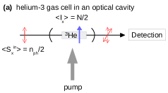
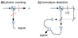
Figure 1: Overview of the set-up. (a) A centimetric glass cell is filled with a helium-3 gas at room temperature and placed in an optical cavity with axis ${z}$ (horizontal axis in the figure). The Stokes spin of light and the atomic spins (nuclear and metastable) are linearly polarized along ${x}$ (vertical axis in the figure). The cavity mode polarized along ${y}$, initially empty, is populated by the Faraday effect due to the quantum fluctuations of the metastable spins along ${z}$ during its propagation in the gas. It is measured continuously outside the cavity by one of the following two methods: (b) the photons leaking out of the cavity polarized along ${y}$ are separated from those polarized along ${x}$ by a polarizing beam-splitter and then detected in the photon counting regime. (c) Outside the cavity, a homodyne detection of one quadrature of the outgoing field polarized along ${y}$ is carried out, using as local oscillator the outgoing field polarized along ${x}$ (whose polarization has been previously rotated with a half-wave plate to bring it along ${y}$).

The considered physical system is shown in figure 1. A cell filled with a partially polarized gas of a few mbar of pure helium-3 atoms is placed inside an optical cavity. While the majority of atoms remain in the singlet ground state $1^{1}S$ of helium, a weak discharge brings a tiny fraction of the atoms, usually $\simeq 10^{-6}$, into the metastable triplet state 2${}^{3}S$. On the one hand, the cavity is driven by a laser beam propagating along the cavity axis ${z}$ and linearly polarized in the direction ${x}$, which is also the direction of polarization of the atomic sample, to excite the 2${}^{3}S-2^{3}P$ transition with a large frequency detuning; on the other hand, atoms in the metastable state 2${}^{3}S$ (of electronic and nuclear hyperfine spin) are coupled to atoms in the ground state (of purely nuclear spin) by metastability exchange collisions; remarkably, although each exchange collision is individually incoherent, this leads to a well-defined macroscopic coupling between the corresponding collective spins DupontRoc ; LaloeDupontLeduc . As the Faraday interaction with the metastable atoms causes the polarization of the light initially directed along ${x}$ to rotate slightly around the ${z}$ axis, by an angle proportional to the component of the collective metastable spins along ${z}$ as we will see, a continuous destructive measurement of the polarization component along ${y}$ of the field leaking out of the cavity (i) by counting photons as indicated in figure 1b or (ii) by homodyne detection as in figure figure 1c, ultimately performs a non-demolition continuous quantum measurement of the collective nuclear spin along ${z}$ of helium-3 atoms in the ground state.

In the rest of this section, by a semi-classical treatment of the spin fluctuations around their expectation values in the stationary state, we reduce our complex physical system to the simpler one of three coupled collective spins, of which section 3 will give a quantum description.

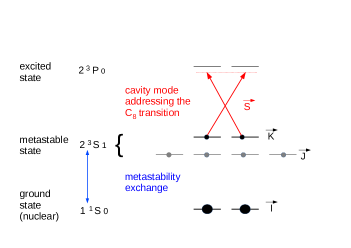
Figure 2: Relevant energy levels of the ³He atoms (the Zeeman sublevels correspond to the choice of ${z}$ as the quantization axis, the atoms being polarized along ${x}$). The cavity mode polarized along ${x}$ excites the transition $C_{8}$ between the level $F=1/2$ of the metastable state 2${}^{3}S_{1}$ and the highest energy level $F=1/2$ of the excited state 2${}^{3}P$, with a negative frequency detuning much larger in absolute value than the Doppler half-width of the excited state (of the order of 1 GHz), so that the velocity class resonant with the laser is almost empty, but much smaller than the 6.74 GHz hyperfine splitting in the metastable state (and a fortiori than the fine splitting 2${}^{3}P_{1}-2{}^{3}P_{0}$ of 29.6 GHz in the excited state), so that the metastable level $F=3/2$ is very weakly affected by the laser. (Note: The frequency separation does not make it possible to largely satisfy these two constraints, and we cannot exclude that the coupling of $F=3/2$ to the field has a small effect on the squeezing dynamics; we neglect it here but we could take it into account with a more complete than our minimal model Hamiltonian (2), like that of reference Dantan2007 ). The six sublevels of the 2${}^{3}S_{1}$ metastable state are coupled to the two (purely nuclear) sublevels of the $1^{1}S_{0}$ ground state by metastability exchange collisions.

The relevant atomic structure of the ³He atom and the transitions excited by the cavity field are shown in figure 2. We call $\vec{I}$ the collective nuclear spin in the ground state, $\vec{J}$ and $\vec{K}$ the collective spins associated with the hyperfine manifolds $F=3/2$ and $F=$ 1/2 in the metastable state. For light propagating along ${z}$, we introduce the Stokes spin Dantan2007 built from the creation and annihilation operators of a photon in the linearly polarized cavity modes along ${x}$ and ${y}$:

$$S_{x}=\frac{1}{2}\left(c_{x}^{\dagger}c_{x}-c_{y}^{\dagger}c_{y}\right)\quad;\quad S_{y}=\frac{1}{2}\left(c_{x}^{\dagger}c_{y}+c_{y}^{\dagger}c_{x}\right)\quad;\quad S_{z}=\frac{1}{2\mathrm{i}}\left(c_{x}^{\dagger}c_{y}-c_{y}^{\dagger}c_{x}\right)\,.$$ (1)

We assume for simplicity that the cell is uniformly illuminated by the cavity mode. Within the limit of a large detuning and a weak saturation of the atomic transition by the field, the excited state 2${}^{3}P$ can be eliminated adiabatically and the interaction Hamiltonian between the metastable spin $\vec{K}$ and the Stokes spin $\vec{S}$ takes the Faraday form Dantan2007 :

$$H=\hbar\chi K_{z}S_{z}$$ (2)

which is none other than the lightshift operator of Zeeman sublevels in the metastable level $F=1/2$, as we can clearly see from the form of $S_{z}$ in footnote 4. The coupled nonlinear equations describing the evolution of the mean spins are given in A, see equations (108)-(110). Besides the evolution due to the Faraday Hamiltonian (2) and to the metastability exchange collisions, they include the contribution of the usual Liouvillian terms in the quantum master equation describing the injection of a polarized coherent field along ${x}$ in the cavity and the losses due to the output mirror, whose combined effect leads to $\langle S_{x}\rangle=n_{\rm ph}/2$ in the stationary state in the absence of atoms, $n_{\rm ph}$ being the average number of photons in the polarized mode along ${x}$. These equations are then linearized around a partially polarized stationary solution (115)-(116), and the fluctuations of the spin $\vec{J}$ and the collective alignment tensor in $F=3/2$ are eliminated adiabatically to obtain coupled equations for the fluctuations of the three collective spins $\vec{I}$, $\vec{K}$ and $\vec{S}$, whose stationary mean values are given by:

$$\langle\vec{I}\rangle_{s}=\frac{N}{2}\,\vec{u}_{x}\quad;\quad\langle\vec{K}\rangle_{s}=\frac{n}{2}\,\vec{u}_{x}\quad;\quad\langle\vec{S}\rangle_{s}=\frac{n_{\rm ph}}{2}\,\vec{u}_{x}$$ (3)

Here $\vec{u}_{x}$ is the unit vector along ${x}$, $N$ and $n$ are the effective numbers of ground-state and metastable atoms participating in the dynamics of the collective spins. As we show in A, these effective numbers are renormalized with respect to the total true numbers $N_{\rm cell}$ and $n_{\rm cell}$ in the cell, by polarization dependent factors:

$$N=\eta\,N_{\rm cell}\quad;\quad n=\left(\frac{1-\eta^{2}}{3+\eta^{2}}\right)\eta\,n_{\rm cell}\\$$ (4)

where $\eta\in[0,1]$ is the nuclear polarization, and the semi-classical equations for the fluctuations of the three collective spins are:

$$\frac{\mathrm{d}}{\mathrm{d}t}\delta S_{z} =-\frac{\kappa}{2}\delta S_{z}\quad\quad\quad\quad\quad\quad\quad\quad\quad\>\>\frac{\mathrm{d}}{\mathrm{d}t}\delta S_{y}=-\frac{\kappa}{2}\delta S_{y}+\chi\langle S_{x}\rangle_{s}\delta K_{z}$$ (5)

$$\frac{\mathrm{d}}{\mathrm{d}t}\delta I_{z} =-\gamma_{f}\delta I_{z}+\gamma_{m}\delta K_{z}\quad\quad\quad\quad\quad\quad\frac{\mathrm{d}}{\mathrm{d}t}\delta I_{y}=-\gamma_{f}\delta I_{y}+\gamma_{m}\delta K_{y}$$ (6)

$$\frac{\mathrm{d}}{\mathrm{d}t}\delta K_{z} =-\gamma_{m}\delta K_{z}+\gamma_{f}\delta I_{z}\quad\quad\quad\quad\quad\quad\frac{\mathrm{d}}{\mathrm{d}t}\delta K_{y}=-\gamma_{m}\delta K_{y}+\gamma_{f}\delta I_{y}+\chi\langle K_{x}\rangle_{s}\delta S_{z}$$ (7)

Here, $\kappa$ is the cavity loss rate, $\gamma_{m}$ and $\gamma_{f}$ are the effective metastability exchange rates in the metastable state and in the ground state. The latter depend on the nuclear polarization as below and in figure 3a, and are in the same ratio as the effective atom numbers $N$ and $n$ (4) forming the collective spins:

$${\gamma_{f}=\frac{4+\eta^{2}}{8-\eta^{2}}\,\frac{1-\eta^{2}}{3+\eta^{2}}\,\frac{1}{T}\quad;\quad\gamma_{m}=\frac{4+\eta^{2}}{8-\eta^{2}}\,\frac{1}{\tau}\quad;}\quad\frac{\gamma_{m}}{\gamma_{f}}=\frac{N}{n}\gg 1$$ (8)

the individual metastability exchange collisions rates $1/T$ and $1/\tau$ experienced by an atom in the ground state and in the metastable state being proportional to $n_{\rm cell}$ and $N_{\rm cell}$ respectively, with the same proportionality constant. In figure 3b, we also show the nuclear polarization dependence of the effective Faraday coupling $\Omega_{\alpha}$ (26) between light and the nuclear spin hybridized by the metastable, which controls the spin squeezing rate in (32).

  

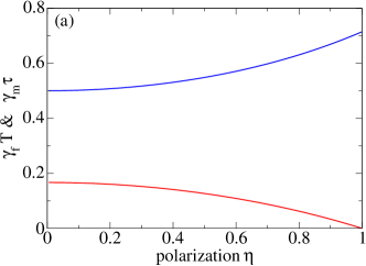
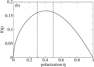
Figure 3: (a) Effective metastability exchange rates $\gamma_{f}$ (lower red curve) and $\gamma_{m}$ (upper blue curve) as given by equation (8) in the ground and metastable states, as functions of nuclear polarization $\eta$, normalized by the metastability exchange collision rates $1/T$ and $1/\tau$ experienced by a ground-state and a metastable atom in the gas. (b) Nuclear polarization dependence of the Faraday frequency $\Omega_{\alpha}$ entering in the rate (32) at which excitations are created by Faraday coupling in the hybridized nuclear bosonic mode, and in the spin squeezing rates (49) and (95), in the limit $\gamma_{f}\ll\gamma_{m}$; more precisely, we plot the factor $f(\eta)=\sqrt{\eta}\frac{1-\eta^{2}}{3+\eta^{2}}$ such that $\Omega_{\alpha}\simeq\Omega(\gamma_{f}/\gamma_{m})^{1/2}=\chi\sqrt{n_{\rm ph}n_{\rm cell}}\sqrt{\frac{n_{\rm cell}}{N_{\rm cell}}}f(\eta)$. When the polarization varies between 0.3 and 0.5 (vertical dashed lines), $f(\eta)$ deviates by 4 % from its maximum $\simeq$ 0.17 reached in $\eta=$ 0.42. It is therefore advantageous to place oneself close to this value of $\eta$ to reduce the temporal drift of $\Omega_{\alpha}$ due to a slight damping of the nuclear polarization during spin squeezing (indeed, the optical pumping process is then interrupted and the lifetime of the polarization is reduced by the presence of the discharge, it becomes of the order of $\gamma_{\alpha}^{-1}$, where $\gamma_{\alpha}$ is the induced decoherence rate of section 4.2.4).

3 Quantum description

In section 2, we have seen that we can model our complex physical system as three coupled collective spins (3): the nuclear spin $\vec{I}$ in the ground state, the spin $\vec{K}$ in the hyperfine level $F=1/2$ of the metastable state and the Stokes spin $\vec{S}$ of the cavity field. In this section, we present the full quantum treatment of this model. After having introduced the Primakoff approximation, we move on to the quantum description of the metastability exchange which couples the nuclear and metastable spins.

3.1 Primakoff approximation and metrological gain due to squeezing

Initially, the collective nuclear spin $\vec{I}$, the collective metastable spin $\vec{K}$ and the Stokes spin $\vec{S}$ of light are polarized along ${x}$, and will remain so throughout the experimental procedure. In the Holstein-Primakoff approximation, which treats the macroscopic spin components along ${x}$ as classical variables, the remaining ${y}$ and ${z}$ components, orthogonal to the mean spins, behave like the quadrature operators (Hermitian and antihermitian parts of annihilation operators, therefore canonically conjugated, $[X,P]=\mathrm{i}/2$) of three bosonic modes $a$, $b$, $c$:

$$\frac{I_{y}}{\sqrt{N}}\stackrel{{\scriptstyle\mbox{\scriptsize{Primakoff}}}}{{\simeq}}X_{a}=\frac{a+a^{\dagger}}{2}\quad ;\quad\frac{K_{y}}{\sqrt{n}}\stackrel{{\scriptstyle\mbox{\scriptsize{Primakoff}}}}{{\simeq}}X_{b}=\frac{b+b^{\dagger}}{2}\quad ;\quad\frac{S_{y}}{\sqrt{n_{\rm ph}}}\stackrel{{\scriptstyle\mbox{\scriptsize{Primakoff}}}}{{\simeq}}X_{c}=\frac{c+c^{\dagger}}{2}$$ (9)

$$\frac{I_{z}}{\sqrt{N}}\stackrel{{\scriptstyle\mbox{\scriptsize{Primakoff}}}}{{\simeq}}P_{a}=\frac{a-a^{\dagger}}{2\mathrm{i}}\quad ;\quad\frac{K_{z}}{\sqrt{n}}\stackrel{{\scriptstyle\mbox{\scriptsize{Primakoff}}}}{{\simeq}}P_{b}=\frac{b-b^{\dagger}}{2\mathrm{i}}\quad ;\quad\frac{S_{z}}{\sqrt{n_{\rm ph}}}\stackrel{{\scriptstyle\mbox{\scriptsize{Primakoff}}}}{{\simeq}}P_{c}=\frac{c-c^{\dagger}}{2\mathrm{i}}$$ (10)

We used the mean values (3) in the normalization. Let us make the link with the exact bosonic representation (1) of Stokes’ spin, writing:

$$\frac{S_{y}}{\sqrt{n_{\rm ph}}}-\mathrm{i}\frac{S_{z}}{\sqrt{n_{\rm ph}}}=\frac{1}{\sqrt{n_{\rm ph}}}c^{\dagger}_{y}c_{x}\stackrel{{\scriptstyle\mbox{\scriptsize{Primakoff}}}}{{\simeq}}c_{y}^{\dagger}\quad\quad;\quad\quad\frac{S_{y}}{\sqrt{n_{\rm ph}}}+\mathrm{i}\frac{S_{z}}{\sqrt{n_{\rm ph}}}=\frac{1}{\sqrt{n_{\rm ph}}}c^{\dagger}_{x}c_{y}\stackrel{{\scriptstyle\mbox{\scriptsize{Primakoff}}}}{{\simeq}}c_{y}$$ (11)

This shows that the creation operator $c^{\dagger}$ in (9)-(10), identified with $c_{y}^{\dagger}$ in Primakoff’s approximation, transfers a photon from the highly populated coherent state cavity mode polarized along ${x}$ into the initially empty cavity mode polarized along ${y}$. In Primakoff’s approximation, the atom-field Faraday coupling Hamiltonian (2) is written:

$$H=\hbar\Omega P_{b}P_{c}\quad\quad\mbox{with}\quad\quad\Omega=\chi\sqrt{nn_{\rm ph}}\,.$$ (12)

As $\chi$ does not depend on the field strength in the cavity, $\Omega^{2}$ is proportional to its intensity. Finally, let’s write in terms of Primakoff variables the parameter $\xi$ of reference Wineland quantifying the level of spin squeezing usable in a magnetometer (the metrological gain is the higher as $\xi$ is the lower, see our footnote 2), $z$ being the maximal squeezing transverse direction to the average spin and the collective nuclear spin being of quantum number $I=N_{\rm cell}/2$:

$$\boxed{\xi^{2}\equiv\frac{2I\,\mbox{Var}_{\rm signal}(I_{z})}{\langle I_{x}\rangle^{2}}=\frac{4\,\mbox{Var}_{\rm signal}(P_{a})}{\eta}}$$ (13)

The nuclear polarization $\eta$ being fixed, and a non-demolition quantum measurement being carried out continuously on the nuclear spin, one must try to minimize the variance of $P_{a}$ conditioned on the measurement signal to be defined, by making it decrease as much as possible below its initial value $1/4$.

3.2 Quantum master equation for metastability exchange

Let us consider in this subsection the evolution of the system due to metastability exchange only ($\chi=0$). In a quantum treatment, the classical equations (6)-(7) become stochastic equations including quantum fluctuations. In Primakoff’s approximation, this gives for the quadratures $X$ in the metastable and fundamental state:

$$\mathrm{d}X_{a}=-\gamma_{f}X_{a}\mathrm{d}t+\sqrt{\gamma_{m}\gamma_{f}}X_{b}\mathrm{d}t+\mathrm{d}X_{a}^{\rm stoch}\quad;\quad\mathrm{d}X_{b}=-\gamma_{m}X_{b}\mathrm{d}t+\sqrt{\gamma_{m}\gamma_{f}}X_{a}\mathrm{d}t+\mathrm{d}X_{b}^{\rm stoch}$$ (14)

where we used the third equality of equation (8). Langevin noises $\mathrm{d}X_{i}^{\rm stoch}$, with $i\in\{a,b\}$, have zero mean, are independent random variables at different times, and have variances and equal-time covariances calculated in reference DantanReinaudi2005 :

$$\langle\mathrm{d}X_{i}^{\rm stoch}\mathrm{d}X_{j}^{\rm stoch}\rangle=D_{ij}\mathrm{d}t\quad\mbox{with}\quad{\underline{\underline{D}}}=\frac{1}{2}\begin{pmatrix}\gamma_{f}&-\sqrt{\gamma_{m}\gamma_{f}}\\ -\sqrt{\gamma_{m}\gamma_{f}}&\gamma_{m}\end{pmatrix}$$ (15)

We have equations of the same form as (14) for the quadratures $P_{i}$, with other Langevin noises $\mathrm{d}P_{i}^{\rm stoch}$, with the same covariance matrix as equation (15) between them but with a covariance matrix with the noises $\mathrm{d}X_{i}^{\rm stoch}$ given by

$$\langle\mathrm{d}X_{i}^{\rm stoch}\mathrm{d}P_{j}^{\rm stoch}\rangle={\cal D}_{ij}\mathrm{d}t\quad\mbox{with}\quad{\underline{\underline{\cal D}}}=\mathrm{i}{\underline{\underline{D}}}$$ (16)

For calculating the mean values and variances of atomic observables, this stochastic formulation is equivalent to a quantum master equation for the atomic density operator $\rho_{\rm at}$ of the two bosonic modes $a$ and $b$:

$$\frac{\mathrm{d}\rho_{\rm at}}{\mathrm{d}t}=C\rho_{\rm at}C^{\dagger}-\frac{1}{2}\{C^{\dagger}C,\rho_{\rm at}\}\quad\mbox{with}\quad C=\sqrt{2\gamma_{f}}a-\sqrt{2\gamma_{m}}b$$ (17)

Indeed, the Langevin stochastic representation of the quantum master equation (17) for any operator $A$ is written

$$\mathrm{d}A=\frac{\mathrm{d}t}{2}\left\{C^{\dagger}[A,C]-[A,C^{\dagger}]C\right\}+\mathrm{d}A^{\rm stoch}\quad\mbox{where}\quad\mathrm{d}A^{\rm stoch}=[C^{\dagger},A]\mathrm{d}B+\mathrm{d}B^{\dagger}[A,C]$$ (18)

and $\mathrm{d}B$ is a Markovian stochastic operator with zero mean, with an equal-time covariance matrix

$$\langle\mathrm{d}B\,\mathrm{d}B^{\dagger}\rangle=\mathrm{d}t\quad;\quad\langle\mathrm{d}B\,\mathrm{d}B\rangle=\langle\mathrm{d}B^{\dagger}\mathrm{d}B^{\dagger}\rangle=\langle\mathrm{d}B^{\dagger}\mathrm{d}B\rangle=0$$ (19)

To be complete, let us sketch another reasoning, which avoids quantum Langevin noises. It suffices to admit that the equations of evolution on the means $\langle X_{i}\rangle$ and $\langle P_{i}\rangle$ taken from (6)-(7) derive from a quantum master equation of the Lindblad form (52). Since these equations are linear, the jump operators $C_{m}$ surrounding $\rho_{\rm at}$ in the quantum master equation are linear combinations of $a$ and $b$, and we recover (17).

3.3 Three-mode quantum master equation

The complete evolution, including the atom-field coupling of Hermitian Hamiltonian (12), metastability exchange and cavity losses, is described by the quantum master equation

$$\frac{\mathrm{d}\rho}{\mathrm{d}t}=\frac{1}{\mathrm{i}\hbar}\left[H,\rho\right]+\kappa\left(c\rho c^{\dagger}-\frac{1}{2}\{c^{\dagger}c,\rho\}\right)+C\rho C^{\dagger}-\frac{1}{2}\{C^{\dagger}C,\rho\}$$ (20)

where $C$ is the jump operator for metastability exchange (17), $\kappa$ is the cavity loss rate, $\gamma_{m}$ and $\gamma_{f}$ are the effective metastability exchange rates in the ground state and in the metastable state.

Initially, the three modes are in vacuum state corresponding to a polarized state for the three spins. For this initial state, the first moments of the quadratures remain zero, and one can obtain a closed system of equations for the second moments. We find that the quadratures $P$ maintain constant variances and zero covariances in the three modes,

$$\langle P_{a}^{2}\rangle(t)=\langle P_{b}^{2}\rangle(t)=\langle P_{c}^{2}\rangle(t)=\frac{1}{4}\quad;\quad\langle P_{a}P_{b}\rangle(t)=\langle P_{a}P_{c}\rangle(t)=\langle P_{b}P_{c}\rangle(t)=0$$ (21)

that the variance $\langle X_{c}^{2}\rangle$ remains bounded and the covariances $\langle X_{a}X_{c}\rangle$ and $\langle X_{b}X_{c}\rangle$ remain zero, while the variances and covariance of the quadratures $X_{a}$ and $X_{b}$, and therefore the number of excitations in the atomic modes, diverge linearly in time, at least as long as the Primakoff approximation is applicable. We give here explicitly only long-time behaviors:

$$\begin{array}[]{ll}\displaystyle\langle X_{a}^{2}\rangle(t)\underset{t\to+\infty}{=}\frac{\gamma_{m}\gamma_{f}}{(\gamma_{m}+\gamma_{f})^{2}}\frac{\Omega^{2}t}{4\kappa}+O(1)&\quad\displaystyle\langle X_{b}^{2}\rangle(t)\underset{t\to+\infty}{=}\frac{\gamma_{f}^{2}}{(\gamma_{m}+\gamma_{f})^{2}}\frac{\Omega^{2}t}{4\kappa}+O(1)\\ &\\ \displaystyle\langle X_{a}X_{b}\rangle(t)\underset{t\to+\infty}{=}\frac{\gamma_{m}^{1/2}\gamma_{f}^{3/2}}{(\gamma_{m}+\gamma_{f})^{2}}\frac{\Omega^{2}t}{4\kappa}+O(1)&\quad\displaystyle\langle X_{c}^{2}\rangle(t)-\frac{1}{4}\underset{t\to+\infty}{\to}\left(\frac{\Omega}{2\kappa}\right)^{2}\left(1-\frac{2\gamma_{m}}{\kappa+2(\gamma_{m}+\gamma_{f})}\right)\end{array}$$ (22)

3.4 One-mode model

In this subsection, we derive a one-mode quantum master equation describing the slow evolution of the nuclear spin within the limit

$$\Gamma_{\rm ex}\ll\gamma_{f}<\gamma_{m}\quad\mbox{and}\quad\Gamma_{\rm ex}\ll\kappa$$ (23)

where $\Gamma_{\rm ex}$ is the rate at which excitations are created under the effect of Faraday coupling in the hybridized nuclear bosonic mode $\alpha$ defined below (it suffices to know here that $\Gamma_{\rm ex}\propto\Omega^{2}$ so that (23) is a weak Faraday coupling limit $\Omega\to 0$). To this end, it is convenient to introduce the bosonic annihilation operators into a cleverly rotated basis, by means of the following linear combinations of the operators $a$ and $b$:

$$\alpha=\sqrt{\frac{\gamma_{m}}{\gamma_{m}+\gamma_{f}}}a+\sqrt{\frac{\gamma_{f}}{\gamma_{m}+\gamma_{f}}}b\quad\quad;\quad\quad\beta=\sqrt{\frac{\gamma_{m}}{\gamma_{m}+\gamma_{f}}}b-\sqrt{\frac{\gamma_{f}}{\gamma_{m}+\gamma_{f}}}a$$ (24)

$\alpha$ and $\beta$ indeed correspond to the eigenmodes of the metastability exchange part of the three-mode quantum master equation (20) (in practice, we have $\gamma_{m}\gg\gamma_{f}$, see equation (8), so that the mode $\beta$ corresponds to the metastable spin slightly hybridized with the spin of the ground state, and $\alpha$ to the nuclear spin slightly hybridized with the metastable spin). While the $\alpha$ mode undergoes a time divergence of its average number of excitations (hence the possibility of defining a rate $\Gamma_{\rm ex}$), the $\beta$ mode is strongly damped and tends towards a stationary value (see the results (21) and (22), which show that $\langle P_{\beta}^{2}\rangle=1/4$ and $\langle X_{\beta}^{2}\rangle=O(1)$ where $X_{\beta}=(\beta+\beta^{\dagger})/2$), which will allow to eliminate it adiabatically, just like the cavity field. In this new basis, the three-mode master equation (20) takes the form

$$\boxed{\frac{\mathrm{d}\rho}{\mathrm{d}t}=\frac{1}{\mathrm{i}\hbar}\left[H,\rho\right]+\kappa\left(c\rho c^{\dagger}-\frac{1}{2}\{c^{\dagger}c,\rho\}\right)+\gamma_{\beta}\left(\beta\rho\beta^{\dagger}-\frac{1}{2}\{\beta^{\dagger}\beta,\rho\}\right)}$$ (25)

where $\gamma_{\beta}\equiv 2(\gamma_{m}+\gamma_{f})$ and, noting $P_{\alpha}=(\alpha-\alpha^{\dagger})/2\mathrm{i}$ and $P_{\beta}=(\beta-\beta^{\dagger})/2\mathrm{i}$ the $P$ quadratures of the new modes,

$$H=\hbar(\Omega_{\alpha}P_{\alpha}+\Omega_{\beta}P_{\beta})P_{c}\quad\mbox{with}\quad\Omega_{\alpha}\equiv\Omega\sqrt{\frac{\gamma_{f}}{\gamma_{m}+\gamma_{f}}}\quad\mbox{and}\quad\Omega_{\beta}{\equiv}\Omega\sqrt{\frac{\gamma_{m}}{\gamma_{m}+\gamma_{f}}}$$ (26)

Reference Sorensen explains in all generality how to perform an adiabatic elimination at the level of the master equation. Here we prefer to carry it out, as in reference CastinMolmer_adel , in the weak Faraday coupling limit $\Omega\to 0$ in the Monte Carlo wave function formalism JOSAB ; CastinDalibard , where the density operator solution of the quantum master equation (25) is obtained by averaging pure states over independent stochastic realizations, each realization corresponding to the deterministic evolution of an unnormalized state vector $|\psi(t)\rangle$ under the action of the effective non-Hermitian Hamiltonian

$$H_{\rm eff}=H-\frac{\mathrm{i}\hbar}{2}\left(\kappa c^{\dagger}c+\gamma_{\beta}\beta^{\dagger}\beta\right)$$ (27)

interrupted randomly by quantum jumps (discontinuous evolutions $|\psi\rangle\to C|\psi\rangle$) of jump operators

$$C_{c}=\sqrt{\kappa}c\quad\mbox{and}\quad C_{\beta}=\sqrt{\gamma_{\beta}}\beta\,.$$ (28)

In the absence of the coherent coupling $\Omega$ in (26) the hybridized metastable mode and the cavity mode remain in the initial empty state. To first order in $\Omega$, this state is coupled to states with an excitation in the cavity (by the action of $P_{c}$) and with zero or one excitation in the mode of the hybridized metastable (by the action of $P_{\alpha}$ or $P_{\beta}$). We can then truncate the Monte Carlo state vector $|\psi\rangle$ in the Fock basis $\{|n_{\alpha}\rangle_{\rm background}|n_{\beta}\rangle_{\scriptsize\mbox{meta}}|n_{c}\rangle_{\rm cav}\}$ as follows

$$|\psi\rangle=|\psi_{\alpha}^{00}\rangle|0\rangle|0\rangle+|\psi_{\alpha}^{01}\rangle|0\rangle|1\rangle+|\psi_{\alpha}^{11}\rangle|1\rangle|1\rangle$$ (29)

committing an error of norm $O(\Omega^{2})$. Under the effect of the effective Hamiltonian (27), the fast components $|\psi_{\alpha}^{01}\rangle$ and $|\psi_{\alpha}^{11}\rangle$ exponentially join an adiabatic following regime of the slow component $|\psi_{\alpha}^{00}\rangle$ with rates $\kappa/2$ or $(\kappa+\gamma_{\beta})/2$. Hence their adiabatic elimination within the limit (23)

$$|\psi_{\alpha}^{11}\rangle_{\rm adiab}\simeq\frac{\mathrm{i}\Omega_{\beta}}{2(\kappa+\gamma_{\beta})}|\psi_{\alpha}^{00}\rangle\quad\mbox{and}\quad|\psi_{\alpha}^{01}\rangle_{\rm adiab}\simeq\frac{\Omega_{\alpha}}{\kappa}\,P_{\alpha}|\psi_{\alpha}^{00}\rangle$$ (30)

We put the expressions of $|\psi_{\alpha}^{11}\rangle_{\rm adiab}$, $|\psi_{\alpha}^{01}\rangle_{\rm adiab}$ in the Hamiltonian evolution equation of $|\psi_{\alpha}^{00}\rangle$ to obtain

$$\mathrm{i}\hbar\frac{\mathrm{d}}{\mathrm{d}t}|\psi_{\alpha}^{00}\rangle=-\frac{\mathrm{i}\hbar}{2}\left(\Gamma_{\rm ex}P_{\alpha}^{2}+\Gamma_{0}\right)|\psi_{\alpha}^{00}\rangle\equiv H_{\rm eff}^{00}\>|\psi_{\alpha}^{00}\rangle$$ (31)

where we have introduced the rates

$$\boxed{\Gamma_{\rm ex}=\frac{\Omega_{\alpha}^{2}}{\kappa}\quad\mbox{and}\quad\Gamma_{0}=\frac{\Omega_{\beta}^{2}}{4(\kappa+\gamma_{\beta})}}$$ (32)

By studying the effect of the cavity jump operator $C_{c}$ and the metastability exchange jump operator $C_{\beta}$ on the state vector (29), we can interpret the effective Hamiltonian of equation (31). (i) Let us first consider the effect of a cavity jump, which occurs at time $t$ with a rate $\kappa(\langle\psi_{\alpha}^{11}|\psi_{\alpha}^{11}\rangle+\langle\psi_{\alpha}^{01}|\psi_{\alpha}^{01}\rangle)_{\rm adiab}/\langle\psi_{\alpha}^{00}|\psi_{\alpha}^{00}\rangle$. Just after the jump, the state vector, initially in the adiabatic following regime, becomes

$$|\psi(t^{+})\rangle=C_{c}|\psi(t^{-})\rangle_{\rm adiab}\propto|\psi_{\alpha}^{01}(t^{-})\rangle_{\rm adiab}|0\rangle|0\rangle+|\psi_{\alpha}^{11}(t^{-})\rangle_{\rm adiab}|1\rangle|0\rangle$$ (33)

It is the superposition of an unstable component $|1\rangle|0\rangle$ and of a stable component $|0\rangle|0\rangle$. With a probability $\langle\psi_{\alpha}^{11}|\psi_{\alpha}^{11}\rangle_{\rm adiab}$ $/(\langle\psi_{\alpha}^{01}|\psi_{\alpha}^{01}\rangle+\langle\psi_{\alpha}^{11}|\psi_{\alpha}^{11}\rangle)_{\rm adiab}$ the cavity jump is then followed by a metastability exchange jump before the system state vector has time to reach its adiabatic value. In this case, we have a “double jump ”, which ultimately does not affect the component $|\psi_{\alpha}^{00}(t^{-})\rangle$ since

$$C_{\beta}C_{c}|\psi(t^{-})\rangle_{\rm adiab}\propto|\psi_{\alpha}^{00}(t^{-})\rangle|0\rangle|0\rangle$$ (34)

This process contributes to the scalar term (proportional to the identity) in the effective Hamiltonian of equation (31). With the complementary probability $\langle\psi_{\alpha}^{01}|\psi_{\alpha}^{01}\rangle_{\rm adiab}/(\langle\psi_{\alpha}^{01}|\psi_{\alpha}^{01}\rangle+\langle\psi_{\alpha}^{11}|\psi_{\alpha}^{11}\rangle)_{\rm adiab}$ the state vector returns to its adiabatic value before other jumps occur, and is slaved to ${|\psi_{\alpha}^{(01)}(t^{-})\rangle_{\rm adiab}\propto}P_{\alpha}|\psi_{\alpha}^{00}(t^{-})\rangle$, that is, the slow component $|\psi_{\alpha}^{00}(t^{-})\rangle$ has effectively undergone a single quantum jump with a jump operator proportional to $P_{\alpha}$. This process corresponds to the first term, proportional to $P_{\alpha}^{2}$, in the effective Hamiltonian of equation (31). (ii) Suppose next that the jump at time $t$ is a metastability exchange jump, which occurs with a rate $\gamma_{\beta}\langle\psi_{\alpha}^{11}|\psi_{\alpha}^{11}\rangle_{\rm adiab}/\langle\psi_{\alpha}^{00}|\psi_{\alpha}^{00}\rangle$. We verify in this case that the state vector after the jump, $C_{\beta}|\psi(t^{-})\rangle$, is entirely unstable and almost immediately undergoes a second jump, a cavity jump. The total effect corresponds here again to a double jump and to the action of a scalar operator on the slow component. We derive from this discussion the following single jump and double jump rates :

$$\Gamma_{s} = \frac{\kappa(\langle\psi_{\alpha}^{11}|\psi_{\alpha}^{11}\rangle+\langle\psi_{\alpha}^{01}|\psi_{\alpha}^{01}\rangle)_{\rm adiab}}{\langle\psi_{\alpha}^{00}|\psi_{\alpha}^{00}\rangle}\frac{\langle\psi_{\alpha}^{01}|\psi_{\alpha}^{01}\rangle_{\rm adiab}}{(\langle\psi_{\alpha}^{01}|\psi_{\alpha}^{01}\rangle+\langle\psi_{\alpha}^{11}|\psi_{\alpha}^{11}\rangle)_{\rm adiab}}=\Gamma_{\rm ex}\frac{\langle\psi_{\alpha}^{00}|P_{\alpha}^{2}|\psi_{\alpha}^{00}\rangle}{\langle\psi_{\alpha}^{00}|\psi_{\alpha}^{00}\rangle}\equiv\Gamma_{\rm ex}\langle P_{\alpha}^{2}\rangle$$ (35)

$$\Gamma_{d} = \frac{\kappa(\langle\psi_{\alpha}^{11}|\psi_{\alpha}^{11}\rangle+\langle\psi_{\alpha}^{01}|\psi_{\alpha}^{01}\rangle)_{\rm adiab}}{\langle\psi_{\alpha}^{00}|\psi_{\alpha}^{00}\rangle}\frac{\langle\psi_{\alpha}^{11}|\psi_{\alpha}^{11}\rangle_{\rm adiab}}{(\langle\psi_{\alpha}^{01}|\psi_{\alpha}^{01}\rangle+\langle\psi_{\alpha}^{11}|\psi_{\alpha}^{11}\rangle)_{\rm adiab}}+\frac{\gamma_{\beta}\langle\psi_{\alpha}^{11}|\psi_{\alpha}^{11}\rangle_{\rm adiab}}{\langle\psi_{\alpha}^{00}|\psi_{\alpha}^{00}\rangle}=\Gamma_{0}$$ (36)

We finally obtain the one-mode quantum master equation describing the slow evolution of the density operator $\rho_{\alpha}$ of the bosonic mode $\alpha$ (hybridized but almost purely nuclear spin):

$$\boxed{\frac{\mathrm{d}\rho_{\alpha}}{\mathrm{d}t}=C_{s}\rho_{\alpha}C_{s}^{\dagger}-\frac{1}{2}\{C_{s}^{\dagger}C_{s},\rho_{\alpha}\}+C_{d}\rho_{\alpha}C_{d}^{\dagger}-\frac{1}{2}\{C_{d}^{\dagger}C_{d},\rho_{\alpha}\}}$$ (37)

in terms of two quantum jumps, the single jump (cavity only) $C_{s}$ and the double jump (of cavity and metastability exchange in that order or in the other) $C_{d}$:

$$C_{s}=\sqrt{\Gamma_{\rm ex}}P_{\alpha}\quad;\quad C_{d}=\sqrt{\Gamma_{0}}\mathbb{1}$$ (38)

By solving equation (37) for the empty initial state of $\alpha$, we get:

$$\langle X_{\alpha}^{2}\rangle=\frac{1}{4}(1+\Gamma_{\rm ex}t)\quad;\quad\langle P_{\alpha}^{2}\rangle=\frac{1}{4}$$ (39)

which effectively designates $\Gamma_{\rm ex}$ as a rate of creation of excitations in the $\alpha$ mode. Going back to the initial atomic basis (unrotated) and by limiting the state vector (29) to its first term, we recover equation (21) and the first three results of equation (22) of the three-mode model, yet valid at any Faraday coupling $\Omega$, not necessarily infinitesimal. Finally, the average number of photons polarized along ${y}$ leaking out of the cavity per unit of time, given in the one-mode model by $\Gamma_{0}+\Gamma_{\rm ex}/4$ as shown by equation (45), agrees with the exact value $\kappa\langle c^{\dagger}c\rangle_{s}$ where the mean stationary number of $y$-polarized photons in the cavity $\langle c^{\dagger}c\rangle_{s}=\langle X_{c}^{2}\rangle_{s}-1/4$ is the last result of (22).

4 Continuous non-demolition quantum measurement of nuclear spin

The quantum averages calculated in section 3 correspond to the ensemble averages over an infinite number of realizations of the experiment. In this section we study what really interests us, the evolution of the system, in one or more given realizations, conditioned on the results of a continuous measurement on the $y$-polarized light leaking out of the cavity. For this, we return to the formulation in terms of Monte Carlo wave functions, as in section 3, where stochastic trajectories $|\psi(t)\rangle$ corresponding to a particular sequence of quantum jumps reconstruct the density operator of the system conditioned on measurement results CastinDalibard . The precise form of the Monte Carlo jump operators, which is not unique in the stochastic reformulation of a quantum master equation, is then determined by the particular measurements made.

4.1 Squeezing by photon counting

Suppose that we continuously and directly count (by photodetection) the number of $y$-polarized photons leaking out of the cavity (see figure 1b), as proposed in reference Milburn1993 . The jump operator associated with this measurement is $\sqrt{\kappa}c$, so the three-mode quantum master equation (20) is already in the right form to analyze the evolution of the state vector $|\psi(t)\rangle$ conditioned on the measurement.

The same is true within the limit of a weak Faraday coupling, $\Omega\to 0$, which leads to the one-mode model of section 3.4. As the jump operators $C_{d}$ and $C_{s}$ of the quantum master equation (37) both correspond to the cavity loss of a $y$-polarized photon (remember, $C_{d}$ results from a cavity jump immediately followed or preceded by a metastability exchange jump, and $C_{s}$ from a single cavity jump), the measurement cannot distinguish between the two, and the density operator conditioned on a given number $n$ of detected photons is obtained by averaging over realizations having this same total number $n$ of jumps. An unnormalized Monte Carlo state vector having undergone such $n$ jumps during $t$ is written

$$|\psi(t)\rangle=\mathrm{e}^{-\frac{\mathrm{i}}{\hbar}{H}^{00}_{\rm eff}(t-t_{n})}\,C_{\epsilon_{n}}\,\mathrm{e}^{-\frac{\mathrm{i}}{\hbar}{H}^{00}_{\rm eff}(t_{n}-t_{n-1})}\,C_{\epsilon_{n-1}}\ldots\,C_{\epsilon_{1}}\,\,\mathrm{e}^{-\frac{\mathrm{i}}{\hbar}{H}_{\rm eff}^{00}t_{1}}|\psi(0)\rangle$$ (40)

where $\epsilon_{k}\in\{s,d\}$ and $t_{k}$ are the type and time of the $k$ th jump, $H_{\rm eff}^{00}$ is the effective Hamiltonian (31) and we denote the state vector of the one-mode model $|\psi\rangle$ rather than $|\psi_{\alpha}^{00}\rangle$ to simplify. The quantum average of an observable $O$ is obtained by averaging over all possible trajectories, therefore by summing over the number and type of jumps and by integrating over their times:

$$\langle O\rangle(t)=\sum_{n}\int_{0<t_{1}<t_{2}\ldots<t_{n}<t}\mathrm{d}t_{1}\,\mathrm{d}t_{2}\ldots\mathrm{d}t_{n}\,\sum_{(\epsilon_{k})_{1\leq k\leq n}\in\{s,d\}^{n}}\langle\psi(t)|O|\psi(t)\rangle$$ (41)

where the squared norm of each unnormalized state vector $|\psi(t)\rangle$ automatically gives its probability density LiYun . By taking $O=\mathbb{1}$, we deduce the probability that $n$ jumps occurred in the time interval $[0,t]$:

$$\Pi_{n}(t)=\int_{0<t_{1}<t_{2}\ldots<t_{n}<t}\mathrm{d}t_{1}\,\mathrm{d}t_{2}\ldots\mathrm{d}t_{n}\,\sum_{(\epsilon_{k})_{1\leq k\leq n}\in\{s,d\}^{n}}\langle\psi(t)|\psi(t)\rangle$$ (42)

To evaluate (42), we take advantage of the fact that all the jump operators in (40) and their Hermitian conjugates commute with each other and with $H_{\rm eff}^{00}$. By using the identities

$$\sum_{\epsilon_{n}=s,d}\ldots\sum_{\epsilon_{1}=s,d}\left(C_{\epsilon_{n}}^{\dagger}C_{\epsilon_{n}}\ldots C_{\epsilon_{1}}^{\dagger}C_{\epsilon_{1}}\right)=\left(\sum_{\epsilon_{n}=s,d}C_{\epsilon_{n}}^{\dagger}C_{\epsilon_{n}}\right)\ldots\left(\sum_{\epsilon_{n}=s,d}C_{\epsilon_{1}}^{\dagger}C_{\epsilon_{1}}\right)=\left(\Gamma_{\rm ex}P_{\alpha}^{2}+\Gamma_{0}\mathbb{1}\right)^{n}$$ (43)

and by injecting a closure relation in the eigenbasis of $P_{\alpha}$ such as $P_{\alpha}|p_{\alpha}\rangle=p_{\alpha}|p_{\alpha}\rangle$, after having integrated over the times $t_{k}$ as allowed by the telescopic product of the evolution operators, we obtain

$$\Pi_{n}(t)=\frac{t^{n}}{n!}\int_{-\infty}^{+\infty}\,\mathrm{d}p_{\alpha}\,\left(\Gamma_{\rm ex}p_{\alpha}^{2}+\Gamma_{0}\right)^{n}\mathrm{e}^{-\Gamma_{\rm ex}p_{\alpha}^{2}t}\mathrm{e}^{-\Gamma_{0}t}\Pi(p_{\alpha},0)=\binom{2n}{n}\frac{(\Gamma_{\rm ex}t/8)^{n}\,\mathrm{e}^{-\Gamma_{0}t}}{(1+\Gamma_{\rm ex}t/2)^{n+1/2}}\,\Phi\left(-n,\frac{1}{2}-n;{\Gamma_{0}}t+\frac{2\Gamma_{0}}{\Gamma_{\rm ex}}\right)$$ (44)

where $\Pi(p_{\alpha},0)$ is the initial probability distribution of $p_{\alpha}$ (a Gaussian with zero mean and variance $1/4$) and $\Phi$ is Kummer’s hypergeometric confluent function ${}_{1}F_{1}$. We notice that (44) is in fact a Gaussian average on $p_{\alpha}$ of a Poisson distribution with parameter $\lambda=(\Gamma_{\rm ex}p_{\alpha}^{2}+\Gamma_{0})t$. We deduce the mean and the variance of the number of photodetections during $t$ :

$$\langle n\rangle=\left(\Gamma_{0}+\frac{1}{4}\Gamma_{\rm ex}\right)t\quad;\quad\mbox{Var}\,n=\langle n\rangle+\frac{(\Gamma_{\rm ex}t)^{2}}{8}$$ (45)

Still using equation (44), we access the probability distribution of $p_{\alpha}$ knowing that $n$ photons were detected in the time interval $[0,t]$, an even function of $p_{\alpha}$:

$$\Pi_{t}(p_{\alpha}|n)=\frac{1}{\Pi_{n}(t)}\frac{t^{n}}{n!}\left(\Gamma_{\rm ex}p_{\alpha}^{2}+\Gamma_{0}\right)^{n}\mathrm{e}^{-\Gamma_{\rm ex}p_{\alpha}^{2}t}\mathrm{e}^{-\Gamma_{0}t}\Pi(p_{\alpha},0)$$ (46)

As expected, it is an even function of $p_{\alpha}$, as photodetection only gives access to the outgoing $y$-polarized field intensity and cannot distinguish between opposite $\pm p_{\alpha}$ values of the $P_{\alpha}$ quadrature of the hybridized nuclear spin along $z$. This results in the squeezing of $P_{\alpha}^{2}$ fluctuations rather than $P_{\alpha}$, which we characterize by the conditional mean and variance of $P_{\alpha}^{2}$ knowing that $n$ photons were detected during $t$, deduced from (46):

$$\langle P_{\alpha}^{2}\rangle_{n}=\frac{(n+1)}{\Gamma_{\rm ex}t}\frac{\Pi_{n+1}(t)}{\Pi_{n}(t)}-\frac{\Gamma_{0}}{\Gamma_{\rm ex}}\quad;\quad{\mbox{Var}_{n}(P_{\alpha}^{2})\equiv\langle P_{\alpha}^{4}\rangle_{n}-\langle P_{\alpha}^{2}\rangle_{n}^{2}=\frac{(n+1)^{2}}{(\Gamma_{\rm ex}t)^{2}}\left[\frac{(n+2)\Pi_{n+2}(t)}{(n+1)\Pi_{n}(t)}-\frac{\Pi^{2}_{n+1}(t)}{\Pi_{n}^{2}(t)}\right]}$$ (47)

Finally, using equation (46), we find for $\Gamma_{\rm ex}t\to+\infty$ that the probability distribution of $p_{\alpha}^{2}$ conditioned on the number $n$ of photodetections is peaked around a value $p_{0}^{2}$ with a conditional variance tending to zero :

$$\boxed{p_{0}^{2}-\frac{1}{4}=\frac{n-\langle n\rangle}{\Gamma_{\rm ex}t}\quad\mbox{hence}\quad\langle P_{\alpha}^{2}\rangle_{n}\underset{\Gamma_{\rm ex}t\to+\infty}{\sim}p_{0}^{2}}\quad;\quad\boxed{\mbox{Var}_{n}(P_{\alpha}^{2})\underset{\Gamma_{\rm ex}t{\to+\infty}}{\sim}\frac{n}{(\Gamma_{\rm ex}t)^{2}}\to 0}$$ (48)

By replacing in this expression $n$ by its mean value and taking into account the value $1/8$ of the variance of $P_{\alpha}^{2}$ in the initial state, we end up with the nuclear spin squeezing rate by photon counting:

$${\boxed{\Gamma_{\rm sq}=\frac{\Gamma_{\rm ex}^{2}}{8(\Gamma_{0}+\frac{1}{4}\Gamma_{\rm ex})}}}$$ (49)

Correspondingly, the conditional probability distribution of $p_{\alpha}$ has two peaks at $\pm p_{0}$ as visible on the Wigner function in figure 5b, obtained by numerical simulation of the conditional evolution of the system over long times in the one-mode model (37). This clearly shows that, in a single realization of the experiment, the continuous photodetection of the $y$-polarized photons leaking out of the cavity makes more and more certain the value of $P_{\alpha}^{2}$, and therefore to a large extent of $I_{z}^{2}$, the square of the component along ${z}$ of the collective nuclear spin, as we clearly see by relating, in the limit $\Omega\to 0$, the conditional moments of $P_{a}^{2}$, that is of $I_{z}^{2}$ to those of $P_{\alpha}^{2}$ :

$$\langle P_{a}^{2}\rangle_{n}=\frac{\gamma_{m}}{\gamma_{f}+\gamma_{m}}\langle P_{\alpha}^{2}\rangle_{n}+\frac{\gamma_{f}/4}{\gamma_{f}+\gamma_{m}}\quad;\quad\mbox{Var}_{n}(P_{a}^{2})=\frac{\gamma_{m}^{2}}{(\gamma_{f}+\gamma_{m})^{2}}\mbox{Var}_{n}(P_{\alpha}^{2})+\frac{\gamma_{f}\gamma_{m}}{(\gamma_{f}+\gamma_{m})^{2}}\langle P_{\alpha}^{2}\rangle_{n}+\frac{\gamma_{f}^{2}/8}{(\gamma_{f}+\gamma_{m})^{2}}$$ (50)

Since the squeezing is on $P_{a}^{2}$ rather than $P_{a}$, the conditional angular distribution of the collective nuclear spin is bimodal (it has, like that of $P_{\alpha}$, two well-separated peaks provided $\gamma_{f}/\gamma_{m}\ll(2p_{0})^{2}$); these structures, which are narrower than the standard quantum limit, still allow for a more accurate angular pointing than in the unsqueezed state. We therefore redefine metrological gain (13) by replacing in the right-hand side of this equation the conditional variance of $P_{a}$ by the square of the halfwidth $\delta P_{a}$ of the peaks centered at $\pm P_{a,0}$ of the conditional probability distribution of $P_{a}$, then equating the center $P_{a,0}^{2}$ and the width $\delta(P_{a}^{2})$ of the distribution of $P_{a}^{2}$ with the conditional mean and standard deviation of $P_{a}^{2}$:

$$\xi^{2}=\frac{4(\delta P_{a})^{2}}{\eta}=\frac{(2P_{a,0}\delta P_{a})^{2}}{\eta P_{a,0}^{2}}=\frac{[\delta(P_{a}^{2})]^{2}}{\eta P_{a,0}^{2}}=\frac{\mbox{Var}_{n}(P_{a}^{2})}{\eta\langle P_{a}^{2}\rangle_{n}}$$ (51)

Note that this expression cannot be deduced from the method of moments explained in section II.B.6 of reference PezzeRMP taking $P_{a}^{2}$ as estimator, because the effect of the unitary transformation $\exp(2\mathrm{i}\theta X_{a})$ (in practice, a precession of the nuclear spin around a magnetic field along $y$) is not to shift the peak in the distribution of $P_{a}^{2}$ but to split it into two peaks centered at $(P_{a,0}\pm\theta)^{2}$.

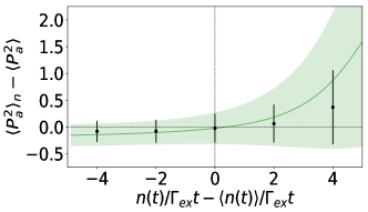
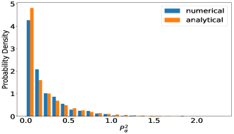
(a)   (b)

Figure 4: Squeezing of $P_{a}^{2}$ by photon counting at short times: $\Gamma_{\rm ex}t=15$, where $\Gamma_{\rm ex}$ is the rate (32) of creation of excitations in the hybridized nuclear bosonic mode $\alpha$. (a) Conditional mean and standard deviation of the squared nuclear spin quadrature $P_{a}^{2}$ knowing that $n$ photons were detected in the time interval $[0,t]$, as functions of this number $n$. The standard deviation is plotted as a confidence interval. The unconditional mean $\langle P_{a}^{2}\rangle=1/4$ is independent of time, see equation (21). Black dots and error bars: numerical simulation of the 3-mode model with 3000 realizations; green line and colored area: analytical predictions taken from equations (44), (47) and (50) of the one-mode model. In practice, the black points are obtained after averaging over classes of values of $n$ centered on these points (in a given class, the trajectories have close photodetection numbers $n$ but independent histories for the metastability exchange jumps which the experimenter cannot access). 3-mode model parameters: $\Omega/\kappa=1/3$, $\gamma_{m}/\kappa=1/10$, $\gamma_{f}/\kappa=1/1000$ (so that $\Gamma_{\rm ex}/\kappa=1/909$), $n_{a}^{\rm max}=64,n_{b}^{\rm max}=n_{c}^{\rm max}=8$. This corresponds to $\Gamma_{0}/\Gamma_{\rm ex}=12\,500/601\simeq 20.8$ and $\Gamma_{\rm sq}/\Gamma_{\rm ex}=601/101\,202\simeq 1/168$ where $\Gamma_{\rm sq}$ is the squeezing rate (49). (b) For the class centered on $n=\langle n(t)\rangle$, histogram of the conditional values of $P_{\alpha}^{2}$. Blue bars: numerical simulation of the three-mode model; orange bars: analytical predictions taken from equation (46) of the one-mode model.

Finally, we carry out a numerical verification of these analytical predictions in the three-mode model. In figure 4a, we plot the conditional mean of the square $P_{a}^{2}$ of the nuclear spin quadrature knowing that $n$ photodetections occurred in the time interval $[0,t]$, with $\Gamma_{\rm ex}t=15$ (black dots), depending on this number $n$. The ensemble of realizations is divided into 5 classes corresponding to a number of photodetections falling within a given interval, and the black dots are obtained by averaging over the realizations in the same class. The numerical results are close to the analytical predictions taken from (47) and (50) and plotted in green, except in the extreme classes which include a too low number of realizations. On the other hand, the asymptotic analytical predictions (48), not shown, would be in disagreement with the simulations of the two models because the time $t=15/\Gamma_{\rm ex}$ is not long enough, it is much less than the squeezing time $1/\Gamma_{\rm sq}$. In figure 4b, we plot the conditional probability distribution of $P_{\alpha}^{2}$ corresponding to the central class of figure 4a; there is also good agreement between one-mode analytical calculation and three-mode numerical simulation.

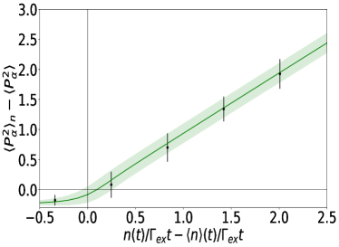
(a)

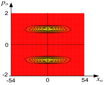
(b)

Figure 5: Squeezing of $P_{\alpha}^{2}$ by photon counting at long times, $\Gamma_{\rm ex}t=1000$, in the one-mode model (37) (this long time would make a simulation in the three-mode model more difficult). (a) Conditional mean and standard deviation of $P_{\alpha}^{2}$ knowing that the number of photodetections $n$ falls in a given class of values, similarly to figure 4a, for 2000 realizations. (b) Wigner distribution of the hybridized nuclear bosonic mode in the quadrature space $(X_{\alpha},P_{\alpha})$ at $\Gamma_{\rm ex}t=1000$, obtained by averaging the dyads $|\psi(t)\rangle\langle\psi(t)|$ whose number of photodetections falls in the 3rd class of (a) (302 trajectories out of 5000 realizations). It has two peak lines but no interference fringes (see note 14).

In figure 5, we are precisely exploring long times in the one-mode model, with $\Gamma_{\rm ex}t=$ 1000 that is $\Gamma_{\rm sq}t\simeq 5.94$. Figure 5a, which is the equivalent of figure 4a, shows that $\langle P_{\alpha}^{2}\rangle_{n}$ is then related to the number of photodetections $n$ as in the analytical prediction (48), i.e. according to the internal bisector in the units of the figure, with a conditional standard deviation (48) roughly constant $\simeq(\Gamma_{0}t)^{1/2}/\Gamma_{\rm ex}t\simeq 1/(\Gamma_{\rm sq}t)^{1/2}$ because $\Gamma_{0}$ is here $\gg\Gamma_{\rm ex}$.

4.2 Squeezing by homodyne detection

We now assume that the $y$-polarized photons leaking out of the cavity are continuously measured by homodyne detection Wiseman2002 , as in figure 1c. We must first find the stochastic equations giving the evolution of the system state vector conditioned on homodyne detection, since the jump operators appearing naturally in (25) or (37) of the three-mode or one-mode quantum master equation are unsuitable. We then present some analytical results obtained in the one-mode model and then in the three-mode model, before briefly discussing the effect of the finite coherence time of metastable atoms. In order to obtain these results, we used the fact that, for the vacuum initial state considered here, the conditional state vector is given exactly at all times by a Gaussian ansatz KlausGauss , whatever the number of modes of the model, in presence or absence of decoherence.

4.2.1 Suitable stochastic formulation of the quantum master equation

A general quantum master equation of the Lindblad form Lindblad

$$\frac{\mathrm{d}\rho}{\mathrm{d}t}=\frac{1}{\mathrm{i}\hbar}\left[H,\rho\right]+\sum_{m}C_{m}\rho C_{m}^{\dagger}-\frac{1}{2}\{C_{m}^{\dagger}C_{m},\rho\}$$ (52)

with $H$ the Hermitian part of the Hamiltonian and $C_{m}$ the jump operators, can be rewritten in an equivalent way by adding an arbitrary constant to the jump operators and/or by mixing them by any linear unitary combination. In order to take into account a homodyne detection on the outgoing field, we form, from a jump operator $C_{m}$ corresponding to a photodetection, the two “homodyne ”  jump operators $D_{m,\pm}$ CastinDalibard

$$D_{m,+}=\frac{\mu\mathbb{1}+C_{m}}{\sqrt{2}}\quad;\quad D_{m,-}=\frac{\mu\mathbb{1}-C_{m}}{\sqrt{2}}$$ (53)

where $\mu^{2}$ has the dimensions of a frequency. The measurement of the difference in the jump rates $D^{\dagger}_{+}D_{+}-D^{\dagger}_{-}D_{-}$ then gives access to a quadrature of $C_{m}$. Thus, for $\mu$ real and $C_{m}$ corresponding to the cavity jump operator $C_{c}$, see equation (28), the difference between the numbers of photons $N_{\pm}$ detected during the short time interval $\Delta t$ in the two output channels of figure 1c, which by definition constitutes the homodyne signal,

$$N_{+}=(D_{c,+}^{\dagger}D_{c,+}^{\phantom{\dagger}})\,\Delta t\quad;\quad N_{-}=(D_{c,-}^{\dagger}D_{c,-}^{\phantom{\dagger}})\,\Delta t\quad;\quad\frac{N_{+}-N_{-}}{2\,\mu}=\frac{c+c^{\dagger}}{2}\sqrt{\kappa}\Delta t$$ (54)

gives access to $X_{c}$  ; it is indeed this quadrature of the field, conjugated to $P_{c}$ therefore translated by a quantity proportional to $P_{b}$ and to the time under the action of the Hamiltonian $H$ (12), which provides information on $P_{a}$ through metastability exchange collisions. In the case of the quantum master equation with 3 modes (25), one has to apply the doubling procedure (53) a priori only to the jump operator of the cavity. In practice, we will apply it also to the jump operator $C_{\beta}$, that is we will double by homodyning all the jump operators $C_{m}$, in order to avoid the discomfort of a hybrid representation mixing discrete quantum jumps and continuous stochastic evolution, see equation (4.2.1) to come. In the case of the one-mode quantum master equation (37), we need to “homodyne ”  the two jump operators $C_{s}$ and $C_{d}$ anyway, since each of them comes with the loss of a photon in a cavity, as explained in section 3.4.

Within the limit of a large amplitude of the local oscillator $\mu$, we can act as if $\Delta t$ were infinitesimal and represent the evolution of the Monte Carlo wave function, now normalized to unity, by a continuous nonlinear stochastic equation without quantum jumps CastinDalibard ; Helvetica ; Percival in Ito point of view:

$$\mathrm{d}|\phi(t)\rangle =-\frac{\mathrm{i}}{\hbar}H|\phi(t)\rangle\mathrm{d}t-\frac{1}{2}\sum_{m}\left(C_{m}^{\dagger}C_{m}-\langle\phi(t)|C_{m}+C_{m}^{\dagger}|\phi(t)\rangle C_{m}+\frac{1}{4}\langle\phi(t)|C_{m}+C_{m}^{\dagger}|\phi(t)\rangle^{2}\right)|\phi(t)\rangle\mathrm{d}t +\sum_{m}\left(C_{m}-\frac{1}{2}\langle\phi(t)|C_{m}+C_{m}^{\dagger}|\phi(t)\rangle\right)|\phi(t)\rangle\,\mathrm{d}\zeta_{m}(t)$$

where, to each jump operator $C_{m}$ in the initial quantum master equation, we associate a continuous-time stochastic process $\mathrm{d}\zeta_{m}(t)$, with real values, Gaussian, of zero mean, of variance $\mathrm{d}t$, statistically independent of other processes and without memory. At the same level of approximation, the homodyne signal operator (54) is replaced by the sum of its average and a classical noise representing its fluctuations, which is none other than the corresponding $\mathrm{d}\zeta_{m}$ CastinDalibard :

$$\frac{N_{+}-N_{-}}{2\mu}=\frac{\sqrt{\kappa}\langle\phi|c+c^{\dagger}|\phi\rangle}{2}\mathrm{d}t+{\frac{1}{2}}\mathrm{d}\zeta_{c}$$ (56)

In practice, more than the homodyning history, that is the detailed time dependence of the homodyne detection signal, it is its time average over an interval of time $[0,t]$ which is easily accessible in an experiment and allows a post-selection of states (i.e. experimental realizations) in a set of non negligible statistical weight. We thus introduce the integrated signal having the dimension of the root of a frequency,

$$\boxed{\sigma(t)\equiv\frac{N_{+}^{\rm tot}-N_{-}^{\rm tot}}{2\mu t}=\frac{1}{t}\int_{0}^{t}\mathrm{d}t^{\prime}\left[\sqrt{\kappa}\langle\phi(t^{\prime})|X_{c}|\phi(t^{\prime})\rangle+{\frac{1}{2}\frac{\mathrm{d}\zeta_{c}(t^{\prime})}{\mathrm{d}t^{\prime}}}\right]}$$ (57)

and we will calculate in the following the mean and the variance of the quadrature $P_{a}$ of the nuclear spin conditioned on $\sigma$.

4.2.2 Analytical results in the one-mode model

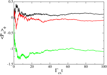
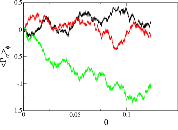
(a)   (b)

Figure 6: In the case of squeezing by continuous homodyne detection: random walk (61) performed in the one-mode model by the quantum average of the quadrature $P_{\alpha}$ of the nuclear spin in a given realization of the experiment. (a) Quantum average as a function of true time $t$ reduced by the rate (32) of creation of excitations for three realizations of the experiment; it is a stretched Brownian motion converging at long times towards a fixed but unpredictable value. (b) Idem as a function of the compact renormalized time $\theta$ (62); this time it is an ordinary Brownian motion but limited to $\theta\leq 1/8$.

Let us explicitly write the stochastic equation (4.2.1) for the one-mode model (37):

$$\mathrm{d}|\phi(t)\rangle=-\frac{\mathrm{d}t}{2}\Gamma_{\rm ex}[P_{\alpha}-\bar{P}_{\alpha}(t)]^{2}|\phi(t)\rangle+\sqrt{\Gamma_{\rm ex}}\mathrm{d}\zeta_{s}(t)[P_{\alpha}-\bar{P}_{\alpha}(t)]|\phi(t)\rangle$$ (58)

with $\bar{P}_{\alpha}(t)\equiv\langle\phi(t)|P_{\alpha}|\phi(t)\rangle$. The highlight is that the jump operator $C_{d}$ proportional to the identity, which added noise in the photon counting detection scheme of section 4.1, gives no contribution and completely disappears in the homodyne case. Indeed, the photons emitted during these jumps come from the component $|1\rangle|1\rangle$ of the state vector (29) containing one excitation $\beta$, which makes them optically incoherent with the light field injected into the cavity, i.e. with the component $|0\rangle|0\rangle$ of (29), in the sense that $|1\rangle|1\rangle$ contributes to $\langle c^{\dagger}c\rangle$ but not to $\langle c+c^{\dagger}\rangle$. So only the stochastic process $\mathrm{d}\zeta_{s}$ associated with the jump operator $C_{s}$ remains. This process coincides with the one $\mathrm{d}\zeta_{c}$ appearing in the homodyne detection signal (56), $\mathrm{d}\zeta_{s}\equiv\mathrm{d}\zeta_{c}$, a fact admitted here but which will be derived in section 4.2.3.

The stochastic equation (58) exhibits a linear noise term and a quadratic deterministic term in the operator $P_{\alpha}$, real in Fourier space. For the initial state considered here, it is thus solved exactly by a Gaussian ansatz on the wave function in momentum representation, real and correctly normalized for the commutation relation $[X_{\alpha},P_{\alpha}]=\mathrm{i}/2$:

$$\langle p_{\alpha}|\phi(t)\rangle=[2\pi u(t)]^{1/4}\exp\{-u(t)[p_{\alpha}-\bar{P}_{\alpha}(t)]^{2}\}$$ (59)

On the other hand, the Gaussianity is lost in the squeezing by photodetection protocol of section 4.1. Using the Ito calculation, we find that $u$ follows a deterministic evolution equation, to be integrated with the initial condition $u(0)=1$:

$$\mathrm{d}u(t)=\Gamma_{\rm ex}\mathrm{d}t\quad\mbox{so that}\quad u(t)=1+\Gamma_{\rm ex}t\quad\mbox{and}\quad\mbox{Var}_{\phi}P_{\alpha}(t)\equiv\frac{1}{4u(t)}=\frac{1}{4}\frac{1}{1+\Gamma_{\rm ex}t}$$ (60)

where we have also given the variance of $P_{\alpha}$ in the state $|\phi\rangle$. On the contrary, the equation for the mean value of $P_{\alpha}$ in $|\phi\rangle$ is purely stochastic, with a diffusion coefficient $D(t)$ depending on time and the initial condition $\bar{P}_{\alpha}(0)=0$:

$$\mathrm{d}\bar{P}_{\alpha}(t)=[2D(t)]^{1/2}\mathrm{d}\zeta_{s}(t)\quad\mbox{with}\quad D(t)=\frac{\Gamma_{\rm ex}}{8u(t)^{2}}=\frac{\Gamma_{\rm ex}}{8(1+\Gamma_{\rm ex}t)^{2}}$$ (61)

As $D(t)$ is of finite integral, $\bar{P}_{\alpha}(t)$ stabilizes asymptotically (at long times) at a fixed value on a single realization, as seen in figure 6, with a variance in the quantum state $\mbox{Var}_{\phi}P_{\alpha}$ tending to $0$. This phenomenon of “stochastic convergence ”  towards an eigenstate of the measured observable (in this case $P_{\alpha}$) is expected in the description of a quantum measurement by a diffusion equation of the state vector Helvetica ; Percival ; Gisin . To show it here, we introduce a renormalized time $\theta$ in terms of which $\bar{P}_{\alpha}$ performs an ordinary Brownian motion with a unity diffusion coefficient, and we notice that this time is bounded:

$$\theta=\int_{0}^{t}\mathrm{d}t^{\prime}D(t^{\prime})=\frac{{\Gamma_{\rm ex}}t}{8(1+\Gamma_{\rm ex}t)}\underset{t\to+\infty}{\to}\theta_{\infty}=\frac{1}{8}$$ (62)

At the renormalized instant $\theta_{\infty}$, $\bar{P}_{\alpha}$ follows a Gaussian law with zero mean and variance $1/4$: $\bar{P}_{\alpha}$ has therefore the same asymptotic probability distribution ($t\to+\infty$) as that of the observable $P_{\alpha}$ in the initial quantum state of the nuclear spin.

We now come to the mean and the variance of $P_{\alpha}$ conditioned on the value $\mathcal{S}$ of the time-integrated homodyning signal $\sigma$ (57). Remarkably, we find that the conditional mean is always proportional to the signal, with a time-dependent proportionality coefficient, and that the conditional variance depends on time but not on the signal:

$$\boxed{\langle P_{\alpha}\rangle_{\sigma=\mathcal{S}}=m(t)\frac{\mathcal{S}}{\sqrt{\Gamma_{\rm ex}}}\quad\mbox{where}\quad{m(t)={\frac{\Gamma_{\rm ex}t}{1+\Gamma_{\rm ex}t}}}\quad;\quad\mbox{Var}_{\sigma=\mathcal{S}}(P_{\alpha})=\mathcal{V}(t)\quad\mbox{where}\quad{\mathcal{V}(t)={\frac{1}{4(1+\Gamma_{\rm ex}t)}}}}$$ (63)

These expressions denote $\Gamma_{\rm ex}$ as the nuclear spin homodyne squeezing rate in the one-mode model that is at weak Faraday coupling:

$${\boxed{\Gamma_{\rm sq}\underset{\Omega\to 0}{\sim}\Gamma_{\rm ex}=\frac{\Omega^{2}\gamma_{f}}{\kappa(\gamma_{m}+\gamma_{f})}}}$$ (64)

In figure 7a, we plot $m(t)$ and $\mathcal{V}(t)$ as functions of the reduced time $\tau=\Gamma_{\rm ex}t$. Just as the quantum variance in a single realization $\mbox{Var}_{\phi}P_{\alpha}$, with which it actually coincides, the conditional variance tends asymptotically towards zero as the inverse of time. In the conditional average, the coefficient $m(t)$ tends towards 1 at long times. To understand this, let’s relate the integrated signal (57) to $\bar{P}_{\alpha}$ using adiabatic expressions (30) in the truncated state vector (29):

$$\sigma(t)=\frac{1}{t}\int_{0}^{t}\mathrm{d}t^{\prime}\left[\sqrt{\Gamma_{\rm ex}}\bar{P}_{\alpha}(t^{\prime})+{\frac{1}{2}\frac{\mathrm{d}\zeta_{s}(t^{\prime})}{\mathrm{d}t^{\prime}}}\right]$$ (65)

As $\bar{P}_{\alpha}(t)$ stabilizes asymptotically on a single realization, and the time average of the noise $\mathrm{d}\zeta_{s}$ tends to zero like $1/t^{1/2}$, $\sigma(+\infty)$ directly gives the value of $\bar{P}_{\alpha}(+\infty)$ up to a constant factor $\sqrt{\Gamma_{\rm ex}}$.

To derive the results (63), we first relate the conditional variance of the operator $P_{\alpha}$ to that of its quantum average in a realization $\bar{P}_{\alpha}$ as follows:

$$\mbox{Var}_{\sigma=\mathcal{S}}(P_{\alpha}) \!\!\!\equiv\!\!\! \langle\,\langle\phi|P_{\alpha}^{2}|\phi\rangle\,\rangle_{\sigma=\mathcal{S}}-\langle\,\langle\phi|{P}_{\alpha}|\phi\rangle\,\rangle_{\sigma=\mathcal{S}}^{2}=\langle\,\langle\phi|P_{\alpha}^{2}|\phi\rangle-\langle\phi|P_{\alpha}|\phi\rangle^{2}\,\rangle_{\sigma=\mathcal{S}}+\langle\bar{P}_{\alpha}^{2}\rangle_{\sigma=\mathcal{S}}-\langle\bar{P}_{\alpha}\rangle^{2}_{\sigma=\mathcal{S}}$$ (66)

$$\!\!\!=\!\!\! \langle\mbox{Var}_{\phi}P_{\alpha}\rangle_{\sigma=\mathcal{S}}+\mbox{Var}_{\sigma=\mathcal{S}}(\bar{P}_{\alpha})={\frac{1}{4}\frac{1}{1+\Gamma_{\rm ex}t}}+\mbox{Var}_{\sigma=\mathcal{S}}(\bar{P}_{\alpha})$$

where we have used expression (60) for the quantum variance of $P_{\alpha}$ in the state $|\phi\rangle$. It therefore remains to determine the conditional probability distribution of $\bar{P}_{\alpha}$ knowing that $\sigma=\mathcal{S}$,

$$P(\bar{P}_{\alpha}=p_{\alpha}|\sigma=\mathcal{S})\equiv\frac{P(\bar{P}_{\alpha}=p_{\alpha},\sigma=\mathcal{S})}{P(\sigma=\mathcal{S})}$$ (67)

The random variable $\bar{P}_{\alpha}(t)$, resulting from Brownian motion (61), has a Gaussian probability distribution; the same applies to the temporal integral of $\bar{P}_{\alpha}$ and to the noise $\mathrm{d}\zeta_{s}$, therefore to the signal $\sigma$ (65) which is their sum. As the variables $\bar{P}_{\alpha}$ and $\sigma$ have zero means, their joint probability distribution is characterized by their covariance matrix, or more directly by its inverse matrix, so that

$$P(\bar{P}_{\alpha}=p_{\alpha}|\sigma=\mathcal{S}) \!\!\!=\!\!\! \frac{\frac{1}{2\pi\sqrt{\langle\bar{P}_{\alpha}^{2}\rangle_{\rm stoch}\langle\sigma^{2}\rangle_{\rm stoch}-\langle\sigma\bar{P}_{\alpha}\rangle_{\rm stoch}^{2}}}\exp\left(-\frac{1}{2}\frac{p_{\alpha}^{2}\langle\sigma^{2}\rangle_{\rm stoch}+\mathcal{S}^{2}\langle\bar{P}_{\alpha}^{2}\rangle_{\rm stoch}-2p_{\alpha}\mathcal{S}\langle\sigma\bar{P}_{\alpha}\rangle_{\rm stoch}}{\langle\bar{P}_{\alpha}^{2}\rangle_{\rm stoch}\langle\sigma^{2}\rangle_{\rm stoch}-\langle\sigma\bar{P}_{\alpha}\rangle_{\rm stoch}^{2}}\right)}{\frac{1}{\sqrt{2\pi\langle\sigma^{2}\rangle_{\rm stoch}}}\exp\left(-\frac{\mathcal{S}^{2}}{2\langle\sigma^{2}\rangle_{\rm stoch}}\right)}$$ (68)

$$\!\!\!=\!\!\! \frac{1}{\sqrt{2\pi\left[\langle\bar{P}_{\alpha}^{2}\rangle_{\rm stoch}-\langle\sigma\bar{P}_{\alpha}\rangle_{\rm stoch}^{2}/\langle\sigma^{2}\rangle_{\rm stoch}\right]}}{\exp\left[-\frac{1}{2}\frac{\left(p_{\alpha}-\mathcal{S}\langle\sigma\bar{P}_{\alpha}\rangle_{\rm stoch}/\langle\sigma^{2}\rangle_{\rm stoch}\right)^{2}}{\langle\bar{P}_{\alpha}^{2}\rangle_{\rm stoch}-\langle\sigma\bar{P}_{\alpha}\rangle_{\rm stoch}^{2}/\langle\sigma^{2}\rangle_{\rm stoch}}\right]}$$

where $\langle\ldots\rangle_{\rm stoch}$ at time $t$ is the average taken over all the realizations of the stochastic process $\mathrm{d}\zeta_{s}(t^{\prime})$ in the time interval $[0,t]$. We deduce that, in equations (63),

$${m(t)}=\sqrt{\Gamma_{\rm ex}}\frac{\langle\sigma(t)\bar{P}_{\alpha}(t)\rangle_{\rm stoch}}{\langle\sigma^{2}(t)\rangle_{\rm stoch}}\quad\mbox{and}\quad{\mathcal{V}(t)=\frac{1}{4(1+\Gamma_{\rm ex}t)}}+\langle\bar{P}_{\alpha}^{2}(t)\rangle_{\rm stoch}-\frac{\langle\sigma(t)\bar{P}_{\alpha}(t)\rangle_{\rm stoch}^{2}}{\langle\sigma^{2}(t)\rangle_{\rm stoch}}$$ (69)

In order to determine their variances and covariance, we write $\sigma(t)$ and $\bar{P}_{\alpha}(t)$ as linear functionals of the stochastic process $\mathrm{d}\zeta_{s}$ and we use the fact that the Langevin forces $\mathrm{d}\zeta_{s}(t)/\mathrm{d}t$ and $\mathrm{d}\zeta_{s}(t^{\prime})/\mathrm{d}t^{\prime}$ have a Dirac correlation function $\delta(t-t^{\prime})$. Let us give the example of the first contribution to $\sigma(t)$:

$$\int_{0}^{t}\mathrm{d}t^{\prime\prime}\bar{P}_{\alpha}(t^{\prime\prime})=\int_{0}^{t}\mathrm{d}t^{\prime\prime}\int_{0}^{t^{\prime\prime}}\mathrm{d}t^{\prime}[2D(t^{\prime})]^{1/2}{\frac{\mathrm{d}\zeta_{s}(t^{\prime})}{\mathrm{d}t^{\prime}}}=\int_{0}^{t}\mathrm{d}t^{\prime}\int_{t^{\prime}}^{t}\mathrm{d}t^{\prime\prime}[2D(t^{\prime})]^{1/2}{\frac{\mathrm{d}\zeta_{s}(t^{\prime})}{\mathrm{d}t^{\prime}}}=\int_{0}^{t}\mathrm{d}t^{\prime}(t-t^{\prime})[2D(t^{\prime})]^{1/2}{\frac{\mathrm{d}\zeta_{s}(t^{\prime})}{\mathrm{d}t^{\prime}}}$$ (70)

where we changed the order of integration on $t^{\prime}$ and $t^{\prime\prime}$ then explicitly integrated on $t^{\prime\prime}$. We end up with the expressions we are looking for (63), the simplicity of which follows from the fact that, in one realization of the experiment, we always have

$$\boxed{\sigma(t)=\sqrt{\Gamma_{\rm ex}}{\frac{1+\Gamma_{\rm ex}t}{\Gamma_{\rm ex}t}}\bar{P}_{\alpha}(t)}$$ (71)

Remarkably, the knowledge of the integrated signal $\sigma(t)$ in a realization of the experiment of duration $t$ is sufficient to prepare the nuclear spin in a well-defined pure Gaussian state (59), with a parameter $u$ given by equation (60) and a mean quadrature $\bar{P}_{\alpha}$ related to the signal by equation (71)

Finally, let us return to the quadrature $P_{a}$ of the unhybridized nuclear spin, which is truly usable in the experiment once the discharge is switched-off in the cell, as shown by expression (13) of the metrological gain in a precession measurement. By inversion of transformation (24) and by limiting equation (29) to its first term (to the dominant order in $\Omega$), it comes

$$\langle P_{a}\rangle_{\sigma=\mathcal{S}}=\left(\frac{\gamma_{m}}{\gamma_{f}+\gamma_{m}}\right)^{1/2}\,\langle P_{\alpha}\rangle_{\sigma=\mathcal{S}}\quad\mbox{and}\quad\mbox{Var}_{\sigma=\mathcal{S}}(P_{a})=\frac{\gamma_{f}}{4(\gamma_{f}+\gamma_{m})}+{\frac{\gamma_{m}}{\gamma_{f}+\gamma_{m}}}\mbox{Var}_{\sigma=\mathcal{S}}(P_{\alpha})$$ (72)

The conditional variance of $P_{a}$ at long times tends towards a nonzero value, although low in practice: this is the intrinsic limit of this nuclear spin squeezing scheme, which uses the metastable state of ³He as an intermediate state.

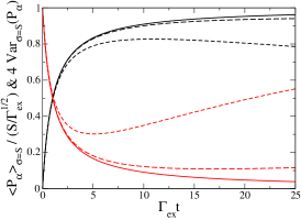
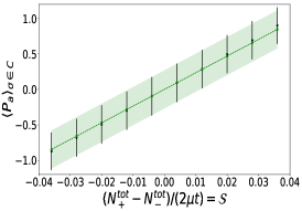
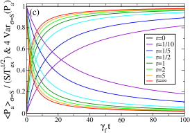
(a) (b) (c)

Figure 7: Nuclear spin squeezing by continuous homodyne measurement. (a) In the one-mode model, mean (in black) and variance (multiplied by 4, in red) of the quadrature $P_{\alpha}$ of the hybridized nuclear spin conditioned on the integrated homodyne signal $\sigma$, as functions of the integration time $t$. Solid lines: analytical expressions (63). Dashed lines: expressions (102) and (103) in the presence of decoherence by de-excitation of metastable atoms at the cell walls (long dashed line: $\epsilon=1/100$, short dashed line: $\epsilon=1/10$, with $\epsilon=\gamma_{\alpha}/\Gamma_{\rm ex}$ and $\gamma_{\alpha}$ the effective decoherence rate (98)). (b) In the three-mode model, for $\Gamma_{\rm ex}t=5$, mean and standard deviation of the quadrature $P_{a}$ of the nuclear spin conditioned on the signal $\sigma$ belonging to a class $C$, the range of values of $\sigma/\sqrt{\Gamma_{\rm ex}}$ having been divided into 10 classes of the same width (the values $\mathcal{S}$ of $\sigma$ are in units of $\Gamma_{\rm ex}^{1/2}$ on the horizontal axis). The standard deviation is plotted as a confidence interval. In black: numerical simulation of the stochastic equation (4.2.1) with $1079$ realizations. Dashed green and colored area: exact results taken from relations (85), (86) and the analytical expression of the conditional probability distribution of $\bar{P}_{a}$ in terms of the variances and covariance (92) similarly to equation (68). The deviation between numerical and analytical results in the extreme classes is attributable to the low numbers of realizations falling in these classes. Parameter values: $\Omega/\kappa=1/10$, $\gamma_{m}/\kappa=1/10$, $\gamma_{f}/\kappa=1/100$, $\Gamma_{\rm ex}/\kappa=1/1000$. (c) In the limit $\Gamma_{\rm ex}\to 0$ at $\Gamma_{\rm ex}/2\gamma_{f}$ fixed of the three-mode model, conditional mean and variance of $P_{a}$ (94) as functions of reduced time $\gamma_{f}t$, for different values of the ratio $r=2\Gamma_{\rm ex}/\gamma_{f}$ (increasing curves: mean, decreasing curves: variance).

4.2.3 Solution of the three-mode model

The study of spin squeezing in the one-mode model is limited to the regime (23) where the squeezing rate $\Gamma_{\rm sq}\sim\Gamma_{\rm ex}$ is the longest timescale in the system. However, it is crucial for applications to see how far we can speed up the squeezing process by increasing $\Gamma_{\rm ex}$ through, for example, the Faraday coupling $\Omega$ of metastable atoms to the cavity field. To this end, we obtain the analytical solution of the three-mode model by using the Gaussian character of the state vector which results, as for the one-mode model, from the initial state considered (the vacuum), from the linearity of the jump operators $C_{m}$ and the quadraticity of the Hamiltonian $H$ in the quadratures of the modes. The stochastic equation (4.2.1) therefore admits as an exact solution the Gaussian ansatz generalizing that of equation (59),

$$\langle p_{\alpha},p_{\beta},x_{c}|\phi(t)\rangle=\phi(\mathbf{q},t)=[8\pi\det\underline{\underline{u}}(t)]^{1/4}\exp\left\{-[\mathbf{q}-\bar{\mathbf{q}}(t)]\cdot\underline{\underline{u}}(t)\,[\mathbf{q}-\bar{\mathbf{q}}(t)]\right\}\equiv\mathrm{e}^{-S}$$ (73)

where $\underline{\underline{u}}$ is a real symmetric 3$\times 3$ matrix, $\bar{\mathbf{q}}$ is a real three-component vector, the coordinates $q_{\alpha}=p_{\alpha}$ and $q_{\beta}=p_{\beta}$ are in Fourier space (eigenbasis of the quadrature $P$) and the coordinate $q_{c}=x_{c}$ is in the “position" space (eigenbasis of the quadrature $X$). The only trick here was to choose as the metastability exchange jump operator $C_{\beta}=\sqrt{\gamma_{\beta}}\,\mathrm{i}\beta$; this choice of phase, which of course does not change the quantum master equation (25), remains legitimate for the evolution conditioned on the homodyne detection of the field because the metastability jumps are not measured. In the mixed representation of the wave function (73), the Hamiltonian $H$ is then purely imaginary and the jump operators are real, hence the real ansatz (73).

To get the equations of motion on $\underline{\underline{u}}$ and $\bar{\mathbf{q}}$, we calculate in two different ways the relative variation $\mathrm{d}\phi(\mathbf{q},t)/\phi(\mathbf{q},t)$ of the wave function, on the one hand by connecting it to the variation $\mathrm{d}S$ of the quantity $S$ in (73), separated into a deterministic part $\mathrm{d}S_{\!d}$ and a noisy part $\mathrm{d}S_{\!b}$, on the other hand by inserting ansatz (73) in the stochastic equation (4.2.1). By identifying the deterministic parts and the noisy parts of the two resulting forms, we obtain

$$-\mathrm{d}S_{\!b} \!\!\!=\!\!\! \gamma_{\beta}^{1/2}\left(\frac{1}{2}\partial_{q_{\beta}}S-q_{\beta}+\bar{q}_{\beta}\right)\mathrm{d}\zeta_{\beta}-\kappa^{1/2}\left(\frac{1}{2}\partial_{q_{c}}S-q_{c}+\bar{q}_{c}\right)\mathrm{d}\zeta_{c}$$ (74)

$$-\mathrm{d}S_{\!d}+\frac{1}{2}(\mathrm{d}S_{\!b})^{2} \!\!\!=\!\!\! (\Omega_{\alpha}q_{\alpha}+\Omega_{\beta}q_{\beta})\frac{\mathrm{d}t}{2}\partial_{q_{c}}S-\frac{\gamma_{\beta}\mathrm{d}t}{2}\left\{q_{\beta}^{2}-\frac{1}{2}+\frac{1}{4}\left[\partial_{q_{\beta}}^{2}S-\left(\partial_{q_{\beta}}S\right)^{2}\right]+\bar{q}_{\beta}\left(\partial_{q_{\beta}}S-2q_{\beta}\right)+\bar{q}_{\beta}^{2}\right\}$$ (75)

$$-\frac{\kappa\mathrm{d}t}{2}\left\{q_{c}^{2}-\frac{1}{2}+\frac{1}{4}\left[\partial_{q_{c}}^{2}S-\left(\partial_{q_{c}}S\right)^{2}\right]+\bar{q}_{c}\left(\partial_{q_{c}}S-2q_{c}\right)+\bar{q}_{c}^{2}\right\}$$

It remains to insert in (75) the expression of $\mathrm{d}S_{\!b}$ taken from (74), by applying Ito’s rule of replacing the squares of the noises by their mean, then identifying the terms of degree 2 in $\mathbf{q}-\bar{\mathbf{q}}$ to obtain the purely deterministic equation linear on $\underline{\underline{u}}$:

$$\begin{array}[]{lll}\mathrm{d}u_{\alpha\alpha}=-\Omega_{\alpha}\mathrm{d}t\,u_{\alpha c}&\displaystyle\mathrm{d}u_{\alpha\beta}=-\frac{\mathrm{d}t}{2}(\gamma_{\beta}u_{\alpha\beta}+\Omega_{\beta}u_{\alpha c}+\Omega_{\alpha}u_{\beta c})&\displaystyle\mathrm{d}u_{\alpha c}=-\frac{\mathrm{d}t}{2}(\kappa u_{\alpha c}+\Omega_{\alpha}u_{cc})\\ &&\\ \mathrm{d}u_{\beta\beta}=-\Omega_{\beta}\mathrm{d}t\,u_{\beta c}+\gamma_{\beta}\mathrm{d}t(1-u_{\beta\beta})&\displaystyle\mathrm{d}u_{\beta c}=-\frac{\mathrm{d}t}{2}[(\gamma_{\beta}+\kappa)u_{\beta c}+\Omega_{\beta}u_{cc}]&\mathrm{d}u_{cc}=\kappa\mathrm{d}t(1-u_{cc})\end{array}$$ (76)

and the terms of degree 1 in $\mathbf{q}-\bar{\mathbf{q}}$ to obtain the stochastic linear equation for $\bar{\mathbf{q}}$:

$$\mathrm{d}\bar{\mathbf{q}}=\frac{1}{2}\begin{pmatrix}0&0&0\\ 0&-\gamma_{\beta}&0\\ \Omega_{\alpha}&\Omega_{\beta}&-\kappa\end{pmatrix}\mathrm{d}t\,\bar{\mathbf{q}}+\frac{1}{2}[\mbox{Id}-\underline{\underline{c}}(t)]\begin{pmatrix}0\\ \gamma_{\beta}^{1/2}\mathrm{d}\zeta_{\beta}(t)\\ -\kappa^{1/2}\mathrm{d}\zeta_{c}(t)\end{pmatrix}$$ (77)

Needless to say, $\bar{\mathbf{q}}$ is the vector of the quantum averages of the variables $q$ in state vector (73); in addition, we have introduced the notation $\underline{\underline{c}}$ for the inverse matrix of $\underline{\underline{u}}$, which is none other than the quantum covariance matrix of $q$ up to a numerical factor. We therefore have:

$$\langle\phi(t)|q_{i}|\phi(t)\rangle=\bar{q}_{i}(t)\quad\mbox{and}\quad\langle\phi(t)|q_{i}q_{j}|\phi(t)\rangle=\bar{q}_{i}(t)\bar{q}_{j}(t)+\frac{1}{4}c_{ij}(t)\quad\forall i,j\in\{\alpha,\beta,c\}\quad\mbox{with}\quad\underline{\underline{c}}(t)=[\underline{\underline{u}}(t)]^{-1}$$ (78)

The differential system (76) is easily integrated for the initial condition $\underline{\underline{u}}(0)=\mathrm{Id}$:

$$u_{\alpha\alpha}(t) = 1+\frac{\Omega_{\alpha}^{2}t}{\kappa}-\frac{2\Omega_{\alpha}^{2}}{\kappa^{2}}\left(1-\mathrm{e}^{-\kappa t/2}\right)$$ (79)

$$u_{\alpha\beta}(t) = \frac{\Omega_{\alpha}\Omega_{\beta}}{\gamma_{\beta}}\left(\frac{1}{\gamma_{\beta}+\kappa}+\frac{1}{\kappa}\right)\left(1-\mathrm{e}^{-\gamma_{\beta}t/2}\right)+\frac{\Omega_{\alpha}\Omega_{\beta}}{\kappa(\kappa-\gamma_{\beta})}\left(\mathrm{e}^{-\kappa t/2}-\mathrm{e}^{-\gamma_{\beta}t/2}\right)+\frac{\Omega_{\alpha}\Omega_{\beta}}{\kappa(\gamma_{\beta}+\kappa)}\left(\mathrm{e}^{-(\gamma_{\beta}+\kappa)t/2}-\mathrm{e}^{-\gamma_{\beta}t/2}\right)$$ (80)

$$u_{\alpha c}(t) = -\frac{\Omega_{\alpha}}{\kappa}\left(1-\mathrm{e}^{-\kappa t/2}\right)$$ (81)

$$u_{\beta\beta}(t) = 1+\frac{\Omega_{\beta}^{2}}{\gamma_{\beta}(\gamma_{\beta}+\kappa)}\left(1-\mathrm{e}^{-\gamma_{\beta}t}\right)-\frac{2\Omega_{\beta}^{2}}{\kappa^{2}-\gamma_{\beta}^{2}}\left(\mathrm{e}^{-\gamma_{\beta}t}-\mathrm{e}^{-(\gamma_{\beta}+\kappa)t/2}\right)$$ (82)

$$u_{\beta c}(t) = -\frac{\Omega_{\beta}}{\gamma_{\beta}+\kappa}\left(1-\mathrm{e}^{-(\gamma_{\beta}+\kappa)t/2}\right)$$ (83)

$$u_{cc}(t) = 1$$ (84)

It would have been different if we had taken as unknown the covariance matrix $\underline{\underline{c}}(t)$, which obeys a Riccati nonlinear differential system RiccatiMabuchi . Since $\bar{\mathbf{q}}$ describes a Brownian motion (partially damped because the friction matrix in (77) has eigenvalues $0$, $\gamma_{\beta}/2$ and $\kappa/2$), and since the homodyne signal averaged over the time interval $[0,t]$ $\sigma$ is deduced by integration, these random variables have a Gaussian statistic and we can reproduce the reasoning of section 4.2.2. We find for the conditional mean and variance of the quadrature $P_{a}$ of the nuclear spin knowing that $\sigma=\mathcal{S}$ (this variance determines the metrological gain (13)):

$$\!\!\!\!\langle P_{a}\rangle_{\sigma=\mathcal{S}} \!\!\!\!=\!\!\!\! \frac{\langle\sigma(t)\bar{P}_{a}(t)\rangle_{\rm stoch}}{\langle\sigma^{2}(t)\rangle_{\rm stoch}}\mathcal{S}$$ (85)

$$\!\!\!\!\mbox{Var}_{\sigma=\mathcal{S}}(P_{a}) \!\!\!\!=\!\!\!\! \frac{1}{4}\left[\frac{\Omega_{\beta}^{2}}{\Omega^{2}}c_{\alpha\alpha}(t)+\frac{\Omega_{\alpha}^{2}}{\Omega^{2}}c_{\beta\beta}(t)-2\frac{\Omega_{\alpha}\Omega_{\beta}}{\Omega^{2}}c_{\alpha\beta}(t)\right]+\langle\bar{P}_{a}^{2}(t)\rangle_{\rm stoch}-\frac{\langle\sigma(t)\bar{P}_{a}(t)\rangle_{\rm stoch}^{2}}{\langle\sigma^{2}(t)\rangle_{\rm stoch}}=\frac{1}{4}-\frac{\langle\sigma(t)\bar{P}_{a}(t)\rangle_{\rm stoch}^{2}}{\langle\sigma^{2}(t)\rangle_{\rm stoch}}$$ (86)

The expression in brackets in equation (86) is the matrix element of $\underline{\underline{c}}(t)$ in the coordinate vector $(\Omega_{\beta}/\Omega,-\Omega_{\alpha}/\Omega,0)$ of direction $a$ in the rotated basis. The first term in the middle-hand side is therefore, up to a factor $4$, the quantum variance of $P_{a}$ in the stochastic state $\phi(t)$, depending on time but, let us recall, independent of the particular realization of $\phi(t)$. The simplified expression in the right-hand side follows from the property (21) on the unconditional mean $\langle P_{a}^{2}\rangle(t)=1/4$ and from the chain of equalities

$$\langle P_{a}^{2}\rangle(t)=\langle\ \langle\phi(t)|P_{a}^{2}|\phi(t)\rangle\ \rangle_{\rm stoch}=\langle\ \langle\phi(t)|P_{a}^{2}|\phi(t)\rangle-\langle\phi(t)|P_{a}|\phi(t)\rangle^{2}+\langle\phi(t)|P_{a}|\phi(t)\rangle^{2}\ \rangle_{\rm stoch}=\langle\mbox{Var}_{\phi(t)}P_{a}\rangle_{\rm stoch}+\langle\bar{P}_{a}^{2}(t)\rangle_{\rm stoch}$$ (87)

To determine the variance and covariance of the random variables $\bar{P}_{a}(t)$ and $\sigma(t)$, it remains to calculate their amplitudes on the stochastic processes $\mathrm{d}\zeta_{\beta}(t^{\prime})$ and $\mathrm{d}\zeta_{c}(t^{\prime})$, formally integrating equation (77) by the method of variation of constants for $\bar{P}_{a}$ and $\bar{X}_{c}$, and proceeding as in equation (70) for $\sigma$:

$$p_{\beta}(t,t^{\prime})=-\frac{1}{2}\gamma_{\beta}^{1/2}\left\{\frac{\Omega_{\beta}}{\Omega}c_{\alpha\beta}(t^{\prime})+\frac{\Omega_{\alpha}}{\Omega}[1-c_{\beta\beta}(t^{\prime})]\mathrm{e}^{-\gamma_{\beta}(t-t^{\prime})/2}\right\}$$ (88)

$$p_{c}(t,t^{\prime})=\frac{1}{2}\kappa^{1/2}\left\{\frac{\Omega_{\beta}}{\Omega}c_{\alpha c}(t^{\prime})-\frac{\Omega_{\alpha}}{\Omega}c_{\beta c}(t^{\prime})\mathrm{e}^{-\gamma_{\beta}(t-t^{\prime})/2}\right\}$$ (89)

$$\sigma_{\beta}(t,t^{\prime})=\frac{(\gamma_{\beta}\kappa)^{1/2}}{2t}\left\{-c_{\alpha\beta}(t^{\prime})[t-t^{\prime}-f_{\kappa}(t-t^{\prime})]\frac{\Omega_{\alpha}}{\kappa}+[1-c_{\beta\beta}(t^{\prime})][f_{\gamma_{\beta}}(t-t^{\prime})-f_{\kappa}(t-t^{\prime})]\frac{\Omega_{\beta}}{\kappa-\gamma_{\beta}}-c_{\beta c}(t^{\prime})f_{\kappa}(t-t^{\prime})\right\}$$ (90)

$$\sigma_{c}(t,t^{\prime})=\frac{1}{2t}-\frac{\kappa}{2t}\left\{-c_{\alpha c}(t^{\prime})[t-t^{\prime}-f_{\kappa}(t-t^{\prime})]\frac{\Omega_{\alpha}}{\kappa}-c_{\beta c}(t^{\prime})[f_{\gamma_{\beta}}(t-t^{\prime})-f_{\kappa}(t-t^{\prime})]\frac{\Omega_{\beta}}{\kappa-\gamma_{\beta}}+[1-c_{cc}(t^{\prime})]f_{\kappa}(t-t^{\prime})\right\}$$ (91)

where $f_{\lambda}(\tau)\equiv[1-\exp(-\lambda\tau/2)]/(\lambda/2)$. We obtain:

$$\langle\sigma(t)\bar{P}_{a}(t)\rangle_{\rm stoch} \!\!\!=\!\!\! \int_{0}^{t}\mathrm{d}t^{\prime}\,[p_{\beta}(t,t^{\prime})\sigma_{\beta}(t,t^{\prime})+p_{c}(t,t^{\prime})\sigma_{c}(t,t^{\prime})]\quad;\quad\langle\sigma^{2}(t)\rangle_{\rm stoch}=\int_{0}^{t}\mathrm{d}t^{\prime}\,[\sigma_{\beta}^{2}(t,t^{\prime})+\sigma_{c}^{2}(t,t^{\prime})]\quad;$$

$$\langle\bar{P}_{a}^{2}(t)\rangle_{\rm stoch} \!\!\!=\!\!\! \int_{0}^{t}\mathrm{d}t^{\prime}\,[p_{\beta}^{2}(t,t^{\prime})+p_{c}^{2}(t,t^{\prime})]$$ (92)

We deduce from these results the long time limits

$$\langle{P}_{a}\rangle_{\sigma=\mathcal{S}}\underset{t\to+\infty}{\to}\left(\frac{\gamma_{m}}{\gamma_{f}+\gamma_{m}}\right)^{1/2}\frac{\mathcal{S}}{\Gamma_{\rm ex}^{1/2}}\quad;\quad\mbox{Var}_{\sigma=\mathcal{S}}({P}_{a})\underset{t\to+\infty}{\to}\frac{1}{4}\frac{\gamma_{f}}{\gamma_{f}+\gamma_{m}}$$ (93)

with which the predictions (72) of the one-mode model, however obtained within the weak coupling limit (23), are in perfect agreement.

As an application of our analytical solution of the three-mode model, let the rate $\Gamma_{\rm ex}$ tend to zero at fixed reduced time $\tau=\Gamma_{\rm ex}t$ while maintaining (unlike the one-mode model) the ratio $\Gamma_{\rm ex}/\gamma_{f}$ to a non-infinitesimal constant value. The physical motivation is clear: in the planned experiments letter , $\gamma_{f}$ and $\Gamma_{\rm ex}$ are of the same order of magnitude but are really much smaller than $\gamma_{m}$ and $\kappa$ (by factors $\approx 10^{-6}$ and $10^{-9}$). We find in this limit:

$${{\boxed{\langle{P}_{a}\rangle_{\sigma=\mathcal{S}}\sim\frac{\Gamma_{\rm sq}t}{1+\Gamma_{\rm sq}t}\frac{\mathcal{S}}{\Gamma_{\rm ex}^{1/2}}\quad\mbox{and}\quad\mbox{Var}_{\sigma=\mathcal{S}}({P}_{a})\sim\frac{1}{4}\frac{1}{1+\Gamma_{\rm sq}t}}}}$$ (94)

where we have introduced the true or generalized squeezing rate

$${\boxed{\Gamma_{\rm sq}\equiv\left(\frac{1}{\Gamma_{\rm ex}}+\frac{2}{\gamma_{f}}\right)^{-1}}}$$ (95)

We find the natural scaling of the signal by $\Gamma_{\rm ex}^{1/2}$ already observed in the one-mode model and the same functional forms in time, but we lose all relation of proportionality of type (71) between integrated signal and quadrature average in a given realization, the conditional variance of $\bar{P}_{a}$ now being $\nequiv 0$. We represent in figure 7c the variation with reduced time $\gamma_{f}t$ of the conditional mean and variance (94) for different values of the ratio $r=2\Gamma_{\rm ex}/\gamma_{f}$. We notice that the squeezing process is all the faster as $r$ is larger, and that it saturates to a limiting behavior. This was predictable, because $\Gamma_{\rm sq}$ is an increasing function of $r$ with finite limit; at a fixed time, the conditional mean (in units of $\mathcal{S}/\Gamma_{\rm ex}^{1/2}$) is therefore an increasing function and the conditional variance a decreasing function of $r$, as seen in figure 7c. More precisely, in the weak coupling limit $\Omega\to 0$, where $r\to 0$, the generalized squeezing rate is equivalent to the rate $\Gamma_{\rm ex}$ of creation of excitations, in agreement with the one-mode model, and within the limit $r\to+\infty$, it saturates to the value $\gamma_{f}/2$. We cannot therefore squeeze faster than at the rate $\gamma_{f}$, which is not surprising: we cannot hope to reduce the fluctuations in nuclear spin before each atom in the ground state has undergone on average at least one metastability exchange collision, the effective rate $\gamma_{f}$ being in practice of the same order of magnitude as the individual rate $1/T$ in equation (8) except in the case of extreme polarization, see figure 3a.

4.2.4 Effect of decoherence

To be complete, we take into account, in the homodyne squeezing scheme, the finite lifetime $(2\gamma_{0})^{-1}$ of the metastable atoms, which de-excite when they reach the cell walls after diffusive motion in the gas. To this end, we add a jump operator $\sqrt{2\gamma_{0}}b$ to the three-mode quantum master equation (20). As the part other than Hermitian Hamiltonian remains quadratic in the quadratures of the modes, it can be put in reduced form by an appropriate rotation of the atomic modes, as we had already done in section 3.4: one simply has to expand $(a,b)$ in the orthonormal eigenbasis of the rate matrix

$$\underline{\underline{\Gamma}}=\begin{pmatrix}2\gamma_{f}&-2\sqrt{\gamma_{f}\gamma_{m}}\\ -2\sqrt{\gamma_{f}\gamma_{m}}&2(\gamma_{0}+\gamma_{m})\end{pmatrix}$$ (96)

with operator-valued coefficients $\alpha$ and $\beta$. The direction $\beta$ remains that of the maximum eigenvalue $\gamma_{\beta}$ of $\underline{\underline{\Gamma}}$, and $\alpha$ that of the minimum eigenvalue $\gamma_{\alpha}$, now nonzero. This leads to the quantum master equation

$$\boxed{\frac{\mathrm{d}\rho}{\mathrm{d}t}=\frac{1}{\mathrm{i}\hbar}\left[\hbar(\Omega_{\alpha}P_{\alpha}+\Omega_{\beta}P_{\beta})P_{c},\rho\right]+\kappa\left(c\rho c^{\dagger}-\frac{1}{2}\{c^{\dagger}c,\rho\}\right)+\gamma_{\alpha}\left(\alpha\rho\alpha^{\dagger}-\frac{1}{2}\{\alpha^{\dagger}\alpha,\rho\}\right)+\gamma_{\beta}\left(\beta\rho\beta^{\dagger}-\frac{1}{2}\{\beta^{\dagger}\beta,\rho\}\right)}$$ (97)

The new expression for Faraday frequencies $\Omega_{\alpha},\Omega_{\beta}$ and rates $\gamma_{\alpha},\gamma_{\beta}$ can be found in B, which also gives the analytical expression of the mean and of the variance of the quadrature $P_{a}$ of the nuclear spin conditioned on the integrated homodyne signal, in all generality. We restrict ourselves here to the physically useful limit $\gamma_{0}\ll\gamma_{m}$ (we still have $\gamma_{f}<\gamma_{m}$). To lowest order in $\gamma_{0}$, the coefficients $\Omega_{\alpha}$, $\Omega_{\beta}$ and $\gamma_{\beta}$ remain unchanged, and we have

$$\gamma_{\alpha}\simeq\frac{2\gamma_{0}\gamma_{f}}{\gamma_{m}+\gamma_{f}}$$ (98)

which is the reduced rate of decoherence in the hybridized nuclear spin. Moreover, we place ourselves in the limit (23), with $\gamma_{\alpha}=O(\Gamma_{\rm ex})$, which allows to evaluate the effect of decoherence using the one-mode model, which is obtained in the same way as in section 3.4. The stochastic equation (58) is completed as follows,

$$\mathrm{d}|\phi(t)\rangle=-\frac{\Gamma_{\rm ex}\mathrm{d}t}{2}(P_{\alpha}-\bar{P}_{\alpha})^{2}|\phi(t)\rangle+\sqrt{\Gamma_{\rm ex}}\mathrm{d}\zeta_{s}(t)(P_{\alpha}-\bar{P}_{\alpha})|\phi(t)\rangle-\frac{\gamma_{\alpha}\mathrm{d}t}{2}(\alpha^{\dagger}\alpha+2\mathrm{i}\bar{P}_{\alpha}\alpha+\bar{P}_{\alpha}^{2})|\phi(t)\rangle+\sqrt{\gamma_{\alpha}}\mathrm{d}\zeta_{\alpha}(t)(\mathrm{i}\alpha+\bar{P}_{\alpha})|\phi(t)\rangle$$ (99)

We have taken care to choose $\gamma_{\alpha}^{1/2}\mathrm{i}\alpha$ as the jump operator of the effective decoherence (the justification is the same as in section 4.2.3, decoherence jumps are not measured), which allows the equation to be solved by the same real Gaussian ansatz (59). This time we find

$$\mathrm{d}u \!\!\!=\!\!\! [\Gamma_{\rm ex}+\gamma_{\alpha}(1-u)]\mathrm{d}t\quad\Longrightarrow\quad{u(\tau)}=1+\frac{1-\exp(-\epsilon\tau)}{\epsilon}$$ (100)

$$\mathrm{d}\bar{P}_{\alpha} \!\!\!=\!\!\! -\frac{1}{2}\gamma_{\alpha}\bar{P}_{\alpha}\mathrm{d}t+\frac{\sqrt{\Gamma_{\rm ex}}\mathrm{d}\zeta_{s}+\sqrt{\gamma_{\alpha}}(u-1)\mathrm{d}\zeta_{\alpha}}{2u}$$ (101)

where we have set $\tau=\Gamma_{\rm ex}t$ and $\epsilon=\gamma_{\alpha}/\Gamma_{\rm ex}$. The same Gaussianity arguments as in 4.2.2 section lead to the same dependencies in the signal $\mathcal{S}$ of the conditional mean and variance,

$$\langle P_{\alpha}\rangle_{\sigma=\mathcal{S}} \!\!\!=\!\!\! m(\tau)\frac{\mathcal{S}}{\sqrt{\Gamma_{\rm ex}}}\quad\mbox{with}\quad m(\tau)=\sqrt{\Gamma_{\rm ex}}\frac{\langle\sigma(t)\bar{P}_{\alpha}(t)\rangle_{\rm stoch}}{\langle\sigma^{2}(t)\rangle_{\rm stoch}}$$ (102)

$$\mbox{Var}_{\sigma=\mathcal{S}}(P_{\alpha}) \!\!\!=\!\!\! \mathcal{V}(\tau)\quad\mbox{with}\quad\mathcal{V}(\tau)=\frac{1}{4}-\frac{\langle\sigma(t)\bar{P}_{\alpha}(t)\rangle_{\rm stoch}^{2}}{\langle\sigma^{2}(t)\rangle_{\rm stoch}}$$ (103)

and the variance and covariance taken over the stochastic processes $\mathrm{d}\zeta_{s}\equiv\mathrm{d}\zeta_{c}$ and $\mathrm{d}\zeta_{\alpha}$,

$$\frac{\langle\sigma^{2}\rangle_{\rm stoch}}{\Gamma_{\rm ex}} \!\!\!=\!\!\! \int_{0}^{\tau}\frac{\mathrm{d}\tau^{\prime}}{\tau^{2}}\left\{\left[{\frac{1}{2}}+\frac{1-\mathrm{e}^{\epsilon(\tau^{\prime}-\tau)/2}}{\epsilon u(\tau^{\prime})}\right]^{2}+\frac{\left[u(\tau^{\prime})-1\right]^{2}}{u^{2}(\tau^{\prime})}\frac{\left[1-\mathrm{e}^{\epsilon(\tau^{\prime}-\tau)/2}\right]^{2}}{\epsilon}\right\}={\frac{\epsilon\tau-2(1-\mathrm{e}^{-\epsilon\tau/2})}{\epsilon^{2}\tau^{2}}+\frac{1}{4\tau}}$$ (104)

$$\frac{\langle\sigma\bar{P}_{\alpha}\rangle_{\rm stoch}}{\sqrt{\Gamma_{\rm ex}}} \!\!\!=\!\!\! \int_{0}^{\tau}\frac{\mathrm{d}\tau^{\prime}}{\tau}\frac{\mathrm{e}^{\epsilon(\tau^{\prime}-\tau)/2}}{2u(\tau^{\prime})}\left\{{\frac{1}{2}}+\frac{1-\mathrm{e}^{\epsilon(\tau^{\prime}-\tau)/2}}{\epsilon u(\tau^{\prime})}+\frac{\left[u(\tau^{\prime})-1\right]^{2}}{u(\tau^{\prime})}\left[1-\mathrm{e}^{\epsilon(\tau^{\prime}-\tau)/2}\right]\right\}={\frac{1-\mathrm{e}^{-\epsilon\tau/2}}{2\epsilon\tau}}$$ (105)

These expressions allow to easily evaluate the effect of decoherence on spin squeezing through the metrological gain (13), see the dashed lines in figure 7a. For the practical case of a weak decoherence $\epsilon\ll 1$ and a time short compared to $1/\gamma_{\alpha}$, they can be expanded to first order in $\epsilon$:

$${\boxed{m(\tau)=\frac{\tau}{1+\tau}-\epsilon\frac{(\tau+3)\tau^{2}}{12(\tau+1)^{2}}+O(\epsilon^{2}\tau^{2})\quad;\quad\mathcal{V}(\tau)=\frac{1}{4(\tau+1)}+\epsilon\frac{(\tau+3/2)\tau^{2}}{12(\tau+1)^{2}}+O(\epsilon^{2}\tau^{2})}}$$ (106)

We then deduces that the optimal squeezing on $P_{\alpha}$ is obtained at a time $t_{\rm opt}\sim(3/\Gamma_{\rm ex}\gamma_{\alpha})^{1/2}$ and corresponds to a conditional variance $\mathcal{V}_{\rm opt}\sim(\gamma_{\alpha}/12\Gamma_{\rm ex})^{1/2}$. Note that in studies of spin squeezing of alkaline gases in cavities, we often introduce the cooperativity $C$ of the coupled atom-field system, defined as the square of the coupling frequency divided by the decay rates of the coupled states Vuletic . In this sense, the cooperativity of the hybridized nuclear spin-field system is equal to

$$C\equiv\frac{\Omega_{\alpha}^{2}}{\kappa\gamma_{\alpha}}=\frac{\Gamma_{\rm ex}}{\gamma_{\alpha}}\simeq\frac{\Omega^{2}}{2\gamma_{0}\kappa}$$ (107)

so that we recover the scaling law of power $-1/2$, usual in alkalis, relating the optimal spin variance to $C$ Vuletic . More generally, the decoherence has a weak effect on the nuclear spin squeezing as long as we stay at short times in front of $t_{\rm opt}$. The reader will find at the end of B an extension of these scaling laws beyond the one-mode model, i.e. for an arbitrary, not infinitesimal ratio $\Gamma_{\rm ex}/\gamma_{f}$; this was retained in the abstract of the article. The link between $\mathcal{V}_{\rm opt}$ and cooperativity (107) is then broken.

Acknowledgements : Alice Sinatra thanks Franck Laloë for helpful discussions. All authors except Yvan Castin are funded by the Horizon 2020 European research and innovation project macQsimal number 820393. Matteo Fadel thanks the Research Fund of the University of Basel for Excellent Junior Researchers.

Appendix A Semi-classical treatment and reduction to three coupled spins

Here we give the nonlinear equations that describe the dynamics of the system in semi-classical theory, and we linearize them for small fluctuations around a partially polarized stationary solution.

Nonlinear semi-classical equations

Starting from the considerations and notations of section 2, we take the average of the Heisenberg equations of motion in the quantum state of the system and perform the decorrelation approximation (called semi-classical in quantum optics) $\langle AB\rangle\simeq\langle A\rangle\langle B\rangle$ where $A$ and $B$ are two operators, to obtain the following nonlinear evolution equations for the expectation values of $\vec{S}$ the Stokes spin of the cavity field, $\vec{I}$ the collective nuclear spin in the ground state, $\vec{J}$ and $\vec{K}$ the collective spins associated with the manifolds $F=3/2$ and $F=1/2$ in the metastable state, and $\vec{\vec{Q}}$ the collective alignment tensor in $F=3/2$, of Cartesian components $Q_{\alpha\beta}$ :

$$\frac{\mathrm{d}\langle S_{x}\rangle}{\mathrm{d}t} =-\frac{\kappa}{2}\left(\langle S_{x}\rangle-\frac{n_{\rm ph}}{2}\right)-\chi\langle K_{z}\rangle\langle S_{y}\rangle \frac{\mathrm{d}\langle S_{y}\rangle}{\mathrm{d}t}=-\frac{\kappa}{2}\langle S_{y}\rangle+\chi\langle K_{z}\rangle\langle S_{x}\rangle \frac{\mathrm{d}\langle S_{z}\rangle}{\mathrm{d}t}=-\frac{\kappa}{2}\langle S_{z}\rangle$$ (108)

$$\frac{\mathrm{d}\langle K_{x}\rangle}{\mathrm{d}t} =\left.\frac{\mathrm{d}\langle K_{x}\rangle}{\mathrm{d}t}\right|_{\rm ME}-\chi\langle K_{y}\rangle\langle S_{z}\rangle \frac{\mathrm{d}\langle K_{y}\rangle}{\mathrm{d}t}=\left.\frac{\mathrm{d}\langle K_{y}\rangle}{\mathrm{d}t}\right|_{\rm ME}+\chi\langle K_{x}\rangle\langle S_{z}\rangle \frac{\mathrm{d}\langle K_{z}\rangle}{\mathrm{d}t}=\left.\frac{\mathrm{d}\langle K_{z}\rangle}{\mathrm{d}t}\right|_{\rm ME}$$ (109)

$$\frac{\mathrm{d}\langle\vec{J}\rangle}{\mathrm{d}t} =\left.\frac{\mathrm{d}\langle\vec{J}\rangle}{\mathrm{d}t}\right|_{\rm ME} \frac{\mathrm{d}\langle Q_{\alpha\beta}\rangle}{\mathrm{d}t}=\left.\frac{\mathrm{d}\langle Q_{\alpha\beta}\rangle}{\mathrm{d}t}\right|_{\rm ME} \frac{\mathrm{d}\langle\vec{I}\rangle}{\mathrm{d}t}=\left.\frac{\mathrm{d}\langle\vec{I}\rangle}{\mathrm{d}t}\right|_{\rm ME}$$ (110)

The terms proportional to the loss rate $\kappa$ of the cavity output mirror make $\langle S_{x}\rangle$ relax towards its stationary value $\langle S_{x}\rangle_{s}=n_{\rm ph}/2$ driven by the laser field polarized along ${x}$ injected into the cavity, and the transverse means $\langle S_{y}\rangle$ and $\langle S_{z}\rangle$ towards zero. The terms proportional to the Faraday coupling $\chi$ between the cavity mode and the spin $\vec{K}$ derive from the Hamiltonian (2). The contribution of metastability exchange collisions (ME) between ground-state and metastable atoms is deduced directly from the quantum master equation for the one-atom density operator of references DupontRoc ; LaloeDupontLeduc by simple multiplication or division by the total number of ground-state atoms $N_{\rm cell}$ or metastable atoms $n_{\rm cell}$ in the cell:

$$\left.\frac{\mathrm{d}\langle\vec{K}\rangle}{\mathrm{d}t}\right|_{\rm ME} =-\frac{7}{9\tau}\langle\vec{K}\rangle+\frac{1}{9\tau}\langle\vec{J}\rangle-\frac{1}{9\tau}\frac{n_{\rm cell}}{N_{\rm cell}}\langle\vec{I}\rangle-\frac{4}{3\tau}\frac{1}{N_{\rm cell}}\langle\vec{\vec{Q}}\rangle\cdot\langle\vec{I}\rangle$$ (111)

$$\left.\frac{\mathrm{d}\langle\vec{J}\rangle}{\mathrm{d}t}\right|_{\rm ME} =-\frac{4}{9\tau}\langle\vec{J}\rangle+\frac{10}{9\tau}\langle\vec{K}\rangle+\frac{10}{9\tau}\frac{n_{\rm cell}}{N_{\rm cell}}\langle\vec{I}\rangle+\frac{4}{3\tau}\frac{1}{N_{\rm cell}}\langle\vec{\vec{Q}}\rangle\cdot\langle\vec{I}\rangle$$ (112)

$$\left.\frac{\mathrm{d}\langle Q_{\alpha\beta}\rangle}{\mathrm{d}t}\right|_{\rm ME} =-\frac{2}{3\tau}\langle Q_{\alpha\beta}\rangle+\frac{1}{9\tau}\frac{1}{N_{\rm cell}}\left(3\frac{\langle I_{\alpha}\rangle\langle\Sigma_{\beta}\rangle+\langle I_{\beta}\rangle\langle\Sigma_{\alpha}\rangle}{2}-\delta_{\alpha\beta}\langle\vec{I}\rangle\cdot\langle\vec{\Sigma}\rangle\right)$$ (113)

$$\left.\frac{\mathrm{d}\langle\vec{I}\rangle}{\mathrm{d}t}\right|_{\rm ME} =-\frac{1}{T}\langle\vec{I}\rangle+\frac{1}{3T}\frac{N_{\rm cell}}{n_{\rm cell}}{(\langle\vec{J}\rangle-\langle\vec{K}\rangle)}$$ (114)

where $\langle\vec{\Sigma}\rangle=\frac{2}{3}\left[\langle\vec{J}\rangle+2\langle\vec{K}\rangle\right]$ is the expectation value of the electron spin in the metastable state. See equations (1.37b), (1.37a), (1.39) and (1.25) of reference LaloeDupontLeduc (taking into account a difference of a factor $6$ in the definition of the alignment tensor), or to equations (VIII.30), (VIII.29), (VIII.32) and (VIII.15) of reference DupontRoc (by adding a Kronecker factor $\delta_{\alpha\beta}$ omitted in (VIII.32)). Here $1/\tau$ and $1/T$, the individual metastability exchange collision rates for an atom in the metastable state and in the ground state, are in the ratio $T/\tau=N_{\rm cell}/n_{\rm cell}$ since, in one unit of time, an equal number of ground-state and metastable atoms have undergone an exchange collision DupontRoc ; LaloeDupontLeduc .

Partially polarized stationary solution

In a polarized stationary state of nuclear polarization $\eta\in[0,1]$,

$$\langle I_{x}\rangle_{s} =\eta\frac{N_{\rm cell}}{2}\quad\>;\quad\langle I_{y}\rangle_{s}=\langle I_{z}\rangle_{s}=0\quad\>;\quad\langle S_{x}\rangle_{s}=\frac{n_{\rm ph}}{2}\quad\>;\quad\langle S_{y}\rangle_{s}=\langle S_{z}\rangle_{s}=0$$ (115)

rotational invariance around ${x}$ axis constrains the mean spins in the metastable state to be aligned along ${x}$, and the mean alignment tensor to be diagonal in the Cartesian basis, with equal eigenvalues in ${y}$ and ${z}$ directions. The system (108)-(110) thus admits a stationary solution where the only nonzero expectation values in the metastable state are:

$$\langle K_{x}\rangle_{s} =\frac{\eta}{2}\frac{1-\eta^{2}}{3+\eta^{2}}n_{\rm cell}\ \ ;\ \ \langle J_{x}\rangle_{s}=\eta\frac{5+\eta^{2}}{3+\eta^{2}}n_{\rm cell}\ \ ;\ \ \langle\Sigma_{x}\rangle_{s}=\frac{4\eta}{3+\eta^{2}}n_{\rm cell}\ \ ;\ \ \langle Q_{yy}\rangle_{s}=\langle Q_{zz}\rangle_{s}=-\frac{1}{2}\langle Q_{xx}\rangle_{s}=-\frac{\eta}{12}\langle\Sigma_{x}\rangle_{s}$$ (116)

Linearized semi-classical equations

We now linearize equations (108)-(110) for classical fluctuations around the stationary solution (115)-(116) by performing the substitution $\langle A\rangle\rightarrow\langle A\rangle_{s}+\delta A$ and treating $\delta A$ to first order. By limiting ourselves to the subspace of transverse fluctuations, that is to say to the directions $\alpha=y,z$ orthogonal to the mean spins, we obtain a closed system:

$$\frac{\mathrm{d}}{\mathrm{d}t}\delta S_{\alpha} =-\frac{\kappa}{2}\delta S_{\alpha}+\chi\delta_{\alpha y}\langle S_{x}\rangle_{s}\delta K_{z}$$ (117)

$$\frac{\mathrm{d}}{\mathrm{d}t}\delta K_{\alpha} =-\frac{7}{9\tau}\delta K_{\alpha}+\frac{1}{9\tau}\delta J_{\alpha}-\frac{2\eta}{3\tau}\delta Q_{\alpha x}-\frac{1}{9T}\left(1+\frac{12}{n_{\rm cell}}\langle Q_{\alpha\alpha}\rangle_{s}\right)\delta I_{\alpha}+\chi\delta_{\alpha y}\langle K_{x}\rangle_{s}\delta S_{z}$$ (118)

$$\frac{\mathrm{d}}{\mathrm{d}t}\delta J_{\alpha} =-\frac{4}{9\tau}\delta J_{\alpha}+\frac{10}{9\tau}\delta K_{\alpha}+\frac{2\eta}{3\tau}\delta Q_{\alpha x}+\frac{10}{9T}\left(1+\frac{6}{5n_{\rm cell}}\langle Q_{\alpha\alpha}\rangle\right)\delta I_{\alpha}$$ (119)

$$\frac{\mathrm{d}}{\mathrm{d}t}\delta Q_{\alpha x} =-\frac{2}{3\tau}\delta Q_{\alpha x}+\frac{\eta}{12\tau}\delta\Sigma_{\alpha}+\frac{1}{6Tn_{\rm cell}}\langle\Sigma_{x}\rangle_{s}\delta I_{\alpha}$$ (120)

$$\frac{\mathrm{d}}{\mathrm{d}t}\delta I_{\alpha} =-\frac{1}{T}\delta I_{\alpha}+\frac{1}{3\tau}{(\delta J_{\alpha}-\delta K_{\alpha})}$$ (121)

Reduction to three coupled collective spins

By setting $\frac{\mathrm{d}}{\mathrm{d}t}\delta J_{\alpha}=0$ in equation (119) and $\frac{\mathrm{d}}{\mathrm{d}t}\delta Q_{\alpha x}=0$ in equation (120), we adiabatically eliminate the fluctuations of the collective spin $\vec{J}$ and of the collective alignment tensor whose evolutions are governed by the metastability exchange only:

$$\delta J_{\alpha}^{\rm adiab}=2\frac{10+\eta^{2}}{8-\eta^{2}}\delta K_{\alpha}+\frac{12\tau}{T}\frac{5+2\eta^{2}}{(3+\eta^{2})(8-\eta^{2})}\delta I_{\alpha}\quad;\quad\delta Q_{\alpha x}^{\rm adiab}=\frac{3\eta}{8-\eta^{2}}\delta K_{\alpha}+\frac{\tau}{T}\frac{\eta(13+\eta^{2})}{(3+\eta^{2})(8-\eta^{2})}\delta I_{\alpha}$$ (122)

The transfer of adiabatic expressions (122) in equations (118) and (121) on $\delta K_{\alpha}$ and $\delta I_{\alpha}$ leads in the body of the article to the reduced system (5)-(7) coupling the fluctuations of the three spins (3), where $\gamma_{f}$ and $\gamma_{m}$, the effective metastability exchange rates between the nuclear spin and the spin $F=1/2$ of the metastable, are given by equation (8).

Appendix B Solution of the three-mode model with decoherence for homodyne detection

Here we give the analytical solution of the three-mode model in the presence of decoherence, see the quantum master equation (97), for an evolution of the system conditioned on a continuous homodyne measurement of the component polarized along $y$ of the field leaking out of the cavity. The value of the coefficients $\gamma_{\alpha}$, $\gamma_{\beta}$, $\Omega_{\alpha}$ and $\Omega_{\beta}$, as well as the annihilation operators $\alpha$ and $\beta$, are deduced from a diagonalization of the rate matrix (96). The rates $\gamma_{\alpha}$ and $\gamma_{\beta}$ are the eigenvalues in ascending order:

$$\gamma_{\alpha,\beta}=\gamma_{m}+\gamma_{f}+\gamma_{0}\mp[(\gamma_{m}+\gamma_{f}+\gamma_{0})^{2}-4\gamma_{f}\gamma_{0}]^{1/2}$$ (123)

In terms of the Faraday frequencies $\Omega_{\alpha}$ and $\Omega_{\beta}$, the corresponding normalized eigenvectors are written as $(\Omega_{\beta}/\Omega,\Omega_{\alpha}/\Omega)$ and $(-\Omega_{\alpha}/\Omega,\Omega_{\beta}/\Omega)$, so that $\alpha=(\Omega_{\beta}a+\Omega_{\alpha}b)/\Omega$ and $\beta=(\Omega_{\beta}b-\Omega_{\alpha}a)/\Omega$ with

$$\Omega_{\alpha}=\frac{\Omega(\gamma_{f}-\gamma_{\alpha}/2)}{[\gamma_{m}\gamma_{f}+(\gamma_{f}-\gamma_{\alpha}/2)^{2}]^{1/2}}\quad;\quad\Omega_{\beta}=\frac{\Omega\sqrt{\gamma_{m}\gamma_{f}}}{[\gamma_{m}\gamma_{f}+(\gamma_{f}-\gamma_{\alpha}/2)^{2}]^{1/2}}$$ (124)

with a choice of sign ensuring that $\alpha\to a$ and $\beta\to b$ when $\gamma_{f}\to 0$ and reproducing (26) when $\gamma_{0}\to 0$. Since the jump operator $C_{\alpha}\propto\alpha$ describes unmeasured processes, we can, as we did for $C_{\beta}$, take it of the form $\sqrt{\gamma_{\alpha}}\mathrm{i}\alpha$ and reuse the real Gaussian ansatz (73) in order to solve the stochastic equation (4.2.1) on the state vector. In the evolution equation for matrix $\underline{\underline{u}}$ that appears in the ansatz, the indices $\alpha$ and $\beta$ now play symmetrical roles and we obtain

$$\begin{array}[]{lll}\mathrm{d}u_{\alpha\alpha}=-\Omega_{\alpha}\mathrm{d}t\,u_{\alpha c}+\gamma_{\alpha}\mathrm{d}t(1-u_{\alpha\alpha})&\displaystyle\mathrm{d}u_{\alpha\beta}=-\frac{\mathrm{d}t}{2}[(\gamma_{\alpha}+\gamma_{\beta})u_{\alpha\beta}+\Omega_{\beta}u_{\alpha c}+\Omega_{\alpha}u_{\beta c}]&\displaystyle\mathrm{d}u_{\alpha c}=-\frac{\mathrm{d}t}{2}[(\gamma_{\alpha}+\kappa)u_{\alpha c}+\Omega_{\alpha}u_{cc}]\\ &&\\ \mathrm{d}u_{\beta\beta}=-\Omega_{\beta}\mathrm{d}t\,u_{\beta c}+\gamma_{\beta}\mathrm{d}t(1-u_{\beta\beta})&\displaystyle\mathrm{d}u_{\beta c}=-\frac{\mathrm{d}t}{2}[(\gamma_{\beta}+\kappa)u_{\beta c}+\Omega_{\beta}u_{cc}]&\mathrm{d}u_{cc}=\kappa\mathrm{d}t(1-u_{cc})\end{array}$$ (125)

whose solution for the initial condition $\underline{\underline{u}}(0)=\mathrm{Id}$ is written

$$u_{\alpha\alpha}(t)= 1+\frac{\Omega_{\alpha}^{2}}{\gamma_{\alpha}(\kappa+\gamma_{\alpha})}\left(1-\mathrm{e}^{-\gamma_{\alpha}t}\right)-\frac{2\Omega_{\alpha}^{2}}{\kappa^{2}-\gamma_{\alpha}^{2}}\left(\mathrm{e}^{-\gamma_{\alpha}t}-\mathrm{e}^{-(\kappa+\gamma_{\alpha})t/2}\right)$$ (126)

$$u_{\alpha\beta}(t)= {\frac{\Omega_{\alpha}\Omega_{\beta}}{\gamma_{\alpha}+\gamma_{\beta}}\left(\frac{1}{\kappa+\gamma_{\alpha}}+\frac{1}{\kappa+\gamma_{\beta}}\right)\left(1-\mathrm{e}^{-(\gamma_{\alpha}+\gamma_{\beta})t/2}\right)+\frac{\Omega_{\alpha}\Omega_{\beta}}{(\kappa-\gamma_{\beta})(\kappa+\gamma_{\alpha})}\left(\mathrm{e}^{-(\kappa+\gamma_{\alpha})t/2}-\mathrm{e}^{-(\gamma_{\alpha}+\gamma_{\beta})t/2}\right)}$$

$${+\frac{\Omega_{\alpha}\Omega_{\beta}}{(\kappa-\gamma_{\alpha})(\kappa+\gamma_{\beta})}\left(\mathrm{e}^{-(\kappa+\gamma_{\beta})t/2}-\mathrm{e}^{-(\gamma_{\alpha}+\gamma_{\beta})t/2}\right)}$$ (127)

$$u_{\alpha c}(t)= -\frac{\Omega_{\alpha}}{\kappa+\gamma_{\alpha}}\left(1-\mathrm{e}^{-(\kappa+\gamma_{\alpha})t/2}\right)$$ (128)

$$u_{\beta\beta}(t)= 1+\frac{\Omega_{\beta}^{2}}{\gamma_{\beta}(\kappa+\gamma_{\beta})}\left(1-\mathrm{e}^{-\gamma_{\beta}t}\right)-\frac{2\Omega_{\beta}^{2}}{\kappa^{2}-\gamma_{\beta}^{2}}\left(\mathrm{e}^{-\gamma_{\beta}t}-\mathrm{e}^{-(\kappa+\gamma_{\beta})t/2}\right)$$ (129)

$$u_{\beta c}(t)= -\frac{\Omega_{\beta}}{\kappa+\gamma_{\beta}}\left(1-\mathrm{e}^{-(\kappa+\gamma_{\beta})t/2}\right)$$ (130)

$$u_{cc}(t)= \quad 1$$ (131)

The vector of coordinate averages $\bar{\mathbf{q}}$ appearing in ansatz (73) obeys the stochastic equation

$$\mathrm{d}\bar{\mathbf{q}}=\frac{1}{2}\begin{pmatrix}-\gamma_{\alpha}&0&0\\ 0&-\gamma_{\beta}&0\\ \Omega_{\alpha}&\Omega_{\beta}&-\kappa\end{pmatrix}\mathrm{d}t\,\bar{\mathbf{q}}+\frac{1}{2}[\mbox{Id}-\underline{\underline{c}}(t)]\begin{pmatrix}\gamma_{\alpha}^{1/2}\mathrm{d}\zeta_{\alpha}(t)\\ \gamma_{\beta}^{1/2}\mathrm{d}\zeta_{\beta}(t)\\ -\kappa^{1/2}\mathrm{d}\zeta_{c}(t)\end{pmatrix}$$ (132)

The unconditional expectation value $\langle P_{a}^{2}\rangle$ always being equal to $1/4$, the mean and the variance of $P_{a}$ conditioned on the integrated homodyne signal are still given by equations (85) and (86), by generalizing the expressions (92) of the variances and covariance of the random variables $\bar{P}_{a}(t)$ and $\sigma(t)$ in the case of three independent stochastic processes $\mathrm{d}\zeta_{\alpha}(t^{\prime})$, $\mathrm{d}\zeta_{\beta}(t^{\prime})$ and $\mathrm{d}\zeta_{c}(t^{\prime})$ as follows:

$$\langle\sigma(t)\bar{P}_{a}(t)\rangle_{\rm stoch} =\int_{0}^{t}\mathrm{d}t^{\prime}\,\sum_{\nu\in\{\alpha,\beta,c\}}p_{\nu}(t,t^{\prime})\sigma_{\nu}(t,t^{\prime})\quad;\quad\langle\sigma^{2}(t)\rangle_{\rm stoch}=\int_{0}^{t}\mathrm{d}t^{\prime}\,\sum_{\nu\in\{\alpha,\beta,c\}}\sigma_{\nu}^{2}(t,t^{\prime})\quad;$$

$$\langle\bar{P}_{a}^{2}(t)\rangle_{\rm stoch} =\int_{0}^{t}\mathrm{d}t^{\prime}\,\sum_{\nu\in\{\alpha,\beta,c\}}p_{\nu}^{2}(t,t^{\prime})$$ (133)

with the compact expressions of the corresponding amplitudes

$$p_{\nu}(t,t^{\prime}) =(-1)^{\delta_{\nu c}}\frac{\sqrt{\gamma_{\nu}}}{2\Omega}\left\{\Omega_{\beta}\mathrm{e}^{-\gamma_{\alpha}(t-t^{\prime})/2}[\delta_{\alpha\nu}-c_{\alpha\nu}(t^{\prime})]-\Omega_{\alpha}\mathrm{e}^{-\gamma_{\beta}(t-t^{\prime})/2}[\delta_{\beta\nu}-c_{\beta\nu}(t^{\prime})]\right\}$$ (134)

$$\sigma_{\nu}(t,t^{\prime}) =\frac{\delta_{\nu c}}{2t}+(-1)^{\delta_{\nu c}}\frac{\sqrt{\kappa\gamma_{\nu}}}{2t}\left\{[\delta_{c\nu}-c_{c\nu}(t^{\prime})]f_{\kappa}(t-t^{\prime})+\sum_{\mu\in\{\alpha,\beta\}}\frac{\Omega_{\mu}}{\kappa-\gamma_{\mu}}[\delta_{\mu\nu}-c_{\mu\nu}(t^{\prime})][f_{\gamma_{\mu}}(t-t^{\prime})-f_{\kappa}(t-t^{\prime})]\right\}$$ (135)

The index $\nu$ runs on the three values $\alpha$, $\beta$, $c$ and we set $\gamma_{c}=\kappa$. The $\delta$ function is that of Kronecker, and the $f_{\lambda}$ function is the same as in equations (88)-(91).

The general solution that we have just presented includes the five rates $\gamma_{\alpha},\Gamma_{\rm ex}=\Omega_{\alpha}^{2}/\kappa,\gamma_{f}$ on the one hand, $\gamma_{\beta},\kappa$ on the other hand. The experimentally relevant regime is one where the last two are “infinitely ”  larger than the first three and only contribute through unobservable transient regimes. Mathematically, we reach this limit by making $\gamma_{f}$ tend to zero with $\kappa,\gamma_{m},\gamma_{0}$ and $\Omega$ fixed and with $\tau=\Gamma_{\rm ex}t>0$ fixed. Then the first three rates jointly tend towards zero, that is with finite-limit ratios $\Gamma_{\rm ex}/\gamma_{f}\to\Omega^{2}\gamma_{m}/[\kappa(\gamma_{0}+\gamma_{m})^{2}]$ and $\gamma_{\alpha}/\gamma_{f}\to 2\gamma_{0}/(\gamma_{0}+\gamma_{m})$, the rate $\gamma_{\beta}$ reduces to $\gamma\equiv 2(\gamma_{0}+\gamma_{m})$ and the Faraday coupling $\Omega_{\beta}$ to $\Omega$. All exponential transients disappear in the matrix elements (126)-(130) of $\underline{\underline{u}}$ except those relaxing at the rate $\gamma_{\alpha}$. The amplitudes (134) and (135) on stochastic processes reduce to

$$\frac{p_{\alpha}(t,t^{\prime})}{\sqrt{\Gamma_{\rm ex}}} =\frac{u(\tau^{\prime})-1}{2u(\tau^{\prime})}\sqrt{\epsilon}\,\mathrm{e}^{-\epsilon(\tau-\tau^{\prime})/2} \frac{\sigma_{\alpha}(t,t^{\prime})}{\Gamma_{\rm ex}}=\frac{u(\tau^{\prime})-1}{\tau\,u(\tau^{\prime})}\sqrt{\epsilon}\,\frac{1-\mathrm{e}^{-\epsilon(\tau-\tau^{\prime})/2}}{\epsilon}$$ (136)

$$\frac{p_{\beta}(t,t^{\prime})}{\sqrt{\Gamma_{\rm ex}}} =\frac{\sqrt{\rho}}{(1+\rho)u(\tau^{\prime})}\mathrm{e}^{-\epsilon(\tau-\tau^{\prime})/2} \frac{\sigma_{\beta}(t,t^{\prime})}{\Gamma_{\rm ex}}=\frac{\sqrt{\rho}}{(1+\rho)\tau}\left[\frac{2}{u(\tau^{\prime})}\frac{1-\mathrm{e}^{-\epsilon(\tau-\tau^{\prime})/2}}{\epsilon}+\rho+\frac{\gamma}{\kappa}(\rho-1)\right]$$ (137)

$$\frac{p_{c}(t,t^{\prime})}{\sqrt{\Gamma_{\rm ex}}} =\frac{(1-\rho)}{2(1+\rho)u(\tau^{\prime})}\mathrm{e}^{-\epsilon(\tau-\tau^{\prime})/2} \frac{\sigma_{c}(t,t^{\prime})}{\Gamma_{\rm ex}}=\frac{1}{\tau}\left[\frac{1}{2}+\frac{1-\rho}{1+\rho}\frac{1}{u(\tau^{\prime})}\frac{1-\mathrm{e}^{-\epsilon(\tau-\tau^{\prime})/2}}{\epsilon}+\frac{\rho}{1+\rho}\left(1+\frac{2\gamma}{\kappa}\right)\right]$$ (138)

where $\epsilon=\gamma_{\alpha}/\Gamma_{\rm ex}$ as in section 4.2.4, the function $u(\tau)$ is given by equation (100) and the notation $\rho=\Omega^{2}\kappa/[\gamma(\kappa+\gamma)^{2}]$ generalizes the one of footnote 22. Relations (85) and (86) remain valid, with the new expressions for the variance and covariance

$$\boxed{\frac{\langle\sigma^{2}\rangle_{\rm stoch}}{\Gamma_{\rm ex}}={\frac{\epsilon\tau-2(1-\mathrm{e}^{-\epsilon\tau/2})}{\epsilon^{2}\tau^{2}}+\frac{\Gamma_{\rm ex}}{4\tau\Gamma_{\rm sq}^{\rm gen}}}\quad\quad\mbox{and}\quad\quad\frac{\langle\sigma\bar{P}_{a}\rangle_{\rm stoch}}{\sqrt{\Gamma_{\rm ex}}}={\frac{1-\mathrm{e}^{-\epsilon\tau/2}}{2\epsilon\tau}}}$$ (139)

and the generalized squeezing rate

$$\boxed{\Gamma_{\rm sq}^{\rm gen}=\left[\frac{1}{\Gamma_{\rm ex}}+\frac{2(\gamma_{0}+\gamma_{m})}{\gamma_{f}\gamma_{m}}\right]^{-1}}$$ (140)

which reproduce the variance and covariance (104) and (105) of the one-mode model with decoherence when $\Gamma_{\rm ex}/\gamma_{f}\to 0$ and the spin squeezing rate (95) of the three-mode model without decoherence when $\gamma_{0}\to 0$. The new results can be simplified within the useful limit of weak effective decoherence $\gamma_{\alpha}/\Gamma_{\rm ex}\to 0$ by a order-one expansion in $\epsilon$, which allows to generalize (106) as follows on the conditional mean and variance at a non-infinitesimal value of $\Gamma_{\rm ex}/\gamma_{f}$:

$$m(t) =\frac{\Gamma_{\rm sq}^{\rm gen}t}{1+\Gamma_{\rm sq}^{\rm gen}t}-\frac{\gamma_{\alpha}}{\Gamma_{\rm sq}^{\rm gen}}\frac{(3+\Gamma_{\rm sq}^{\rm gen}t)(\Gamma_{\rm sq}^{\rm gen}t)^{2}}{12(1+\Gamma_{\rm sq}^{\rm gen}t)^{2}}+O[(\gamma_{\alpha}t)^{2}]$$ (141)

$$\mathcal{V}(t) =\frac{1}{4(1+\Gamma_{\rm sq}^{\rm gen}t)}+\frac{\gamma_{\alpha}}{\Gamma_{\rm sq}^{\rm gen}}\frac{(\Gamma_{\rm sq}^{\rm gen}t+3/2)(\Gamma_{\rm sq}^{\rm gen}t)^{2}}{12(1+\Gamma_{\rm sq}^{\rm gen}t)^{2}}+O[(\gamma_{\alpha}t)^{2}]$$ (142)

This generalization simply amounts to replace $\tau$ by $\Gamma_{\rm sq}^{\rm gen}t$ and $\epsilon$ by $\gamma_{\alpha}/\Gamma^{\rm gen}_{\rm sq}$ in the right-hand sides of (106). The optimal squeezing on $P_{a}$ is then obtained at a time $t_{\rm opt}\sim(3/\Gamma_{\rm sq}^{\rm gen}\gamma_{\alpha})^{1/2}$ and corresponds to a conditional variance $\mbox{Var}_{\sigma=\mathcal{S}}^{\rm opt}(P_{a})\sim(\gamma_{\alpha}/12\Gamma_{\rm sq}^{\rm gen})^{1/2}$; the optimal metrological gain is deduced from this by equation (13).

References

- (1) J. MacFall, H. Charles, R. Black, H. Middleton, J. Swartz, B. Saam, B. Driehuys, C. Erickson, W. Happer, G. Cates, G. Johnson, C. Ravin, “Human lung air spaces: potential for MR imaging with hyperpolarized He-3”, Radiology 200 (1996), p. 553.
- (2) C. Gemmel, W. Heil, S. Karpuk, K. Lenz, C. Ludwig, Y. Sobolev, K. Tullney, M. Burghoff, W. Kilian, S. Knappe-Grüneberg, W. Müller, A. Schnabel, F. Seifert, L. Trahms, S. Baeßler, “Ultra-sensitive magnetometry based on free precession of nuclear spins”, Eur. Phys. J. D 57 (2010), p. 303.
- (3) T. R. Gentile, P. J. Nacher, B. Saam, T. G. Walker, “Optically polarized ”, Rev. Mod. Phys. 89 (2017), 045004.
- (4) L. Pezzè, A. Smerzi, M. K. Oberthaler, R. Schmied, P. Treutlein, “Quantum metrology with nonclassical states of atomic ensembles”, Rev. Mod. Phys. 90 (2018), 035005.
- (5) A. Dantan, G. Reinaudi, A. Sinatra, F. Laloë, E. Giacobino, M. Pinard, “Long-Lived Quantum Memory with Nuclear Atomic Spins”, Phys. Rev. Lett. 95 (2005), 123002.
- (6) G. Reinaudi, A. Sinatra, A. Dantan, M. Pinard, “Squeezing and entangling nuclear spins in helium 3”, Journal of Modern Optics 54 (2007), p. 675.
- (7) G. Vasilakis, H. Shen, K. Jensen, M. Balabas, D. Salart, B. Chen, E. Polzik, “Generation of a squeezed state of an oscillator by stroboscopic back-action-evading measurement”, Nature Phys. 11 (2015), p. 389.
- (8) O. Hosten, N. J. Engelsen, R. Krishnakumar, M. A. Kasevich, “Measurement noise 100 times lower than the quantum-projection limit using entangled atoms”, Nature 529 (2016), p. 505.
- (9) Han Bao, Junlei Duan, Shenchao Jin, Xingda Lu, Pengxiong Li, Weizhi Qu, Mingfeng Wang, I. Novikova, E.E. Mikhailov, Kai-Feng Zhao, K. Mølmer, Heng Shen, Yanhong Xiao, “Spin squeezing of atoms by prediction and retrodiction measurements ”, Nature 581 (2020), p. 159.
- (10) M.-Z. Huang, J. A. de la Paz, T. Mazzoni, K. Ott, A. Sinatra, C. L. G. Alzar, J. Reichel, “Self-amplifying spin measurement in a long-lived spin-squeezed state”, preprint, arXiv:2007.01964 (2020).
- (11) D.J. Wineland, J.J. Bollinger, W.M. Itano, D.J. Heinzen, Squeezed atomic states and projection noise in spectroscopy, Phys. Rev. A 50 (1994), p. 67.
- (12) M. Kitagawa, M. Ueda, Squeezed spin states, Phys. Rev. A 47 (1993), p. 5138.
- (13) G. Santarelli, Ph. Laurent, P. Lemonde, A. Clairon, A.G. Mann, S. Chang, A.N. Luiten, C. Salomon, Quantum Projection Noise in an Atomic Fountain: A High Stability Cesium Frequency Standard, Phys. Rev. Lett. 82 (1999), p.4619.
- (14) A. Serafin, M. Fadel, P. Treutlein, A. Sinatra, “Nuclear spin squeezing in Helium-3 by continuous quantum non-demolition measurement”, preprint, hal-03058456 (2020).
- (15) O. Katz, R. Shaham, E. S. Polzik, O. Firstenberg, “Long-Lived Entanglement Generation of Nuclear Spins Using Coherent Light”, Phys. Rev. Lett. 124 (2020), 043602.
- (16) O. Katz, R. Shaham, O. Firstenberg, “Quantum interface for noble-gas spins”, preprint, arXiv:1905.12532 (2019).
- (17) J.M. Geremia, J.K. Stockton, A.C. Doherty, H. Mabuchi, “Quantum Kalman Filtering and the Heisenberg Limit in Atomic Magnetometry ”, Phys. Rev. Lett. 91 (2003), 250801.
- (18) K. Mølmer, L.B. Madsen, “Estimation of a classical parameter with Gaussian probes: Magnetometry with collective atomic spins ”, Phys. Rev. A 70 (2004), 052102.
- (19) R. Jiménez-Martínez, J. Kolodynski, C. Troullinou, V.G. Lucivero, Jia Kong, M.W. Mitchell, “Signal Tracking Beyond the Time Resolution of an Atomic Sensor by Kalman Filtering ”, Phys. Rev. Lett. 120 (2018), 040503.
- (20) Cheng Zhang, K. Mølmer, “Estimating a fluctuating magnetic field with a continuously monitored atomic ensemble ”, Phys. Rev. A 102 (2020), 063716.
- (21) J. Dupont-Roc, “Étude de quelques effets liés au pompage optique en champ faible”, Thesis, Université Paris VI, 1972.
- (22) J. Dupont-Roc, M. Leduc, F. Laloë, “Contribution à l’étude du pompage optique par échange de métastabilité dans 3He. - Première Partie”, Journal de Physique 34 (1973), p. 961.
- (23) J. Cviklinski, A. Dantan, J. Ortalo, M. Pinard, “Conditional squeezing of an atomic alignment”, Phys. Rev. A 76 (2007), 033830.
- (24) A. Kuzmich, L. Mandel, J. Janis, Y. E. Young, R. Ejnisman, N. P. Bigelow, “Quantum nondemolition measurements of collective atomic spin”, Phys. Rev. A 60 (1999), p. 2346.
- (25) F. Reiter, A.S. Sørensen, “Effective operator formalism for open quantum systems”, Phys. Rev. A 85 (2012), 032111.
- (26) Y. Castin, K. Mølmer, “Monte Carlo Wave-Function Analysis of 3D Optical Molasses”, Phys. Rev. Lett. 74 (1995), p. 3772.
- (27) K. Mølmer, Y. Castin, J. Dalibard, “Monte Carlo wave-function method in quantum optics”, J. Opt. Soc. Am. B 10 (1993), p. 524.
- (28) Y. Castin, J. Dalibard, K. Mølmer, “A Wave Function approach to dissipative processes”, AIP Conference Proceedings, Thirteenth International Conference on Atomic Physics (edited by H. Walther, T.W. Hänsch, B. Neizert), 275 (1992).
- (29) H. M. Wiseman, G. J. Milburn, “Quantum theory of field-quadrature measurements”, Phys. Rev. A 47 (1993), p. 642.
- (30) Yun Li, Y. Castin, A. Sinatra, “Optimum Spin Squeezing in Bose-Einstein Condensates with Particle Losses”, Phys. Rev. Lett. 100 (2008), 210401.
- (31) S. Zippilli, D. Vitali, P. Tombesi, J.-M. Raimond, “Scheme for decoherence control in microwave cavities ”, Phys. Rev. A 67 (2003), 052101.
- (32) L. K. Thomsen, S. Mancini, H. M. Wiseman, “Continuous quantum nondemolition feedback and unconditional atomic spin squeezing”, J. Phys. B 35 (2002), p. 4937.
- (33) L.B. Madsen, K. Mølmer, “Spin squeezing and precision probing with light and samples of atoms in the Gaussian description ”, Phys. Rev. A 70 (2004), 052324.
- (34) G. Lindblad, “On the Generators of Quantum dynamical semigroups”, Commun. Math. Phys. 48 (1976), p. 119.
- (35) N. Gisin, “Stochastic quantum dynamics and relativity”, Helv. Phys. Acta 62 (1989), p. 363.
- (36) N. Gisin, I. Percival, “The quantum state diffusion model applied to open systems”, J. Phys. A 25 (1992), p. 5677.
- (37) N. Gisin, “Quantum Measurements and Stochastic Processes”, Phys. Rev. Lett. 52 (1984), p. 1657.
- (38) J.K. Stockton, J.M. Geremia, A.C. Doherty, H. Mabuchi, “Robust quantum parameter estimation: Coherent magnetometry with feedback ”, Phys. Rev. A 69 (2004), 032109.
- (39) H. Tanji-Suzuki, I.D. Leroux, M.H. Schleier-Smith, M. Cetina, A.T. Grier, J. Simon, V. Vuletic, “Interaction between Atomic Ensembles and Optical Resonators: Classical Description ”, Adv. At. Mol. Opt. Phys. 60 (2011), p. 201.