Selling Renewable Utilization Service to Consumers via Cloud Energy Storage

Abstract

This paper proposes a cloud energy storage (CES) model for enabling greater utilization of local renewable generation by building consumers (BCs). As opposed to most existing ES sharing models that the energy storage operator (ESO) leases energy or power capacity to its customers, our CES model suggests the ESO to sell renewable utilization service (RUS) for higher profitability. Particularly, the customers request CES service in the amounts of total local renewable generation they want to shift to supply their demand over the contracted time period. We propose a quadratic price model for the ESO charging its customers by the requested RUS, and formulate their interactions as a Stackelberg game which admits an equilibrium. We prove the CES model outperforms individual ES (IES) model in social welfare. We demonstrate the CES model can provide 2-4 times profit to the ESO and bring higher economic benefits (i.e., cost reduction) to its customers over the existing ES sharing models. Moreover, we show the CES model can achieve near social optima and high ES efficiency (i.e., ES utilization) which are not provided by the other ES models. Particularly, this paper can work as an example how market design and sharing economy can shape the efficiency of energy systems.

I Introduction

Renewable energy is crucial for transitioning to a sustainable and low-carbon energy system [1]. The continuing drop in renewable cost and increase in policy incentives and mandatory targets have boosted renewable installation (e.g., wind and solar power, etc.) around the globe [2, 3]. Whereas blending the volatile and non-dispatchable renewable supply into consumer demand at scale still remains to be resolved due to their asynchronous pace. Energy storage (ES) deems one effective solution to offset the temporal imbalance [4, 5, 6]. However, ES is still expensive and thus paring renewable generators with isolated ES will make the shaped renewable supply cost-prohibitive and raise the levelized cost above high-carbon alternatives [7, 8]. At the same time, despite being capital-intensive, individual or isolated ES installations for renewable integration are usually under-utilized due to the volatility of renewable generation. This poses the possibility of designing appropriate ES business models to enable cost-effective renewable integration.

Sharing economy has manifested in transportation and housing systems [9, 10], suggesting its potential to bring in new technologies into energy systems such as ES [11]. For example, multiple consumers can share their under-utilized private ES with each other, or jointly invest in a central ES [12]. Besides, third-party providers can invest in ES to provide storage service to their customers [13]. The underlying idea is to increase ES utilization and marginal value , thus lowering the economic barriers for ES deployment. Different sharing paradigms can enable different ES business models and applications. Third-party based ES sharing models run by an energy storage operator (ESO) are foreseeable in future energy systems from the profitability and flexibility of providing service at scale. Moreover, ES consumers can overcome the high ES capital cost barriers and embrace greater local renewable utilization. Though the potential economic benefits of ES sharing are clear, achieving the objective is a non-trivial task, and depends on a well-designed ES business model to address the following challenges.

• The ESO and consumers are both self-interested, thus the ES sharing model must admit an equilibrium that ensures both ESO profitability and consumer incentives (i.e., higher economic benefits over individual ES installations).

• As ES is capital-intensive, the operation of the shared ES should be well coordinated so as to improve the ES utilization and economic benefits for the ESO. However, the ES consumers are separate and competitive.

• Due to the diversity of demand and renewable generation, the consumers generally require to charge and discharge the ES in heterogeneous multi-step patterns, which makes it difficult for the ESO to uniformly price the ES service.

Mainly due to the above challenges, most of the existing third-party based ES sharing models fail in securing desirable ESO profit or consumer incentives (see [14, 15, 16, 13, 17]). Typically, [14] proposed a cloud energy storage (CES) model for customers to harvest grid price arbitrage. However, the numeric results report the maximal ESO profit rate is only 4.6% (relative to the ES capital cost) even all consumers commit to paying a service fee equal to individual ES installation (in such setting, no incentive is actually provided to the consumers). [17] also proposed a CES model and addressed the specific problem of ES service pricing. In their model, the ESO charges the consumers by their occupied energy capacity (in $\mathrm{kW}\text{\,}\mathrm{h}$) and power capacity (in $\mathrm{kW}$) with a linear price model. However, we can infer from the numeric results that the ESO profit is mainly from the economics of scale rather than increasing ES utilization through sharing (the ESO purchases ES at scale with a price 40% lower than individual purchase). Besides, [16, 13] proposed a novel third-party based ES sharing model characterized by a two-stage structure: the ESO computes the optimal price to maximize its profit and the customers determine the optimal energy capacity to rent. They also used a similar linear price model by the energy capacity (in $\mathrm{kW}\text{\,}\mathrm{h}$). Notably, a systematic algorithm was proposed to search for the equilibrium price by exploring the problem structures. However, the algorithm seems cumbersome for application. Moreover, the profitability of ESO seems sensitive to scenarios as it depends on the operation of the self-interested and independent consumers over their contracted energy capacity.

In a nutshell, most third-party based ES sharing models can not ensure ESO profitability and consumer incentives. This is mainly caused by the inappropriate (linear) price model used for bargaining. The objective to benefit both the ESO and consumers can be achieved if and only if the ES utilization is enhanced through coordination and sharing. Whereas a linear price model based on energy or power capacity can not direct the coordination of customers over their multi-step charging and discharging of the shared ES. In such setting, the ESO and consumers are likely to fail in bargaining and sharing the potential economic benefits of ES. More importantly, most of such models do not retain social welfare, taking the sharing economy away from its pathway of improving resource efficiency and creating a sustainable future [18].

I-A Contributions

Motivated by the literature, especially [16, 13], this paper studies a third-party based cloud energy storage (CES) model. We seek to achieve ESO profitability and consumer incentives while retaining social welfare. In contrast to most existing works where the ESO profits by leasing energy or power capacity, our CES model suggests the ESO to sell renewable utilization service (RUS) to its consumers. Particularly, the consumers request CES service in the amounts of total local renewable generation they want to shift to supply their demand over the contracted time period. We propose a quadratic price model for the ESO charging its consumers by their requested RUS. The underlying motivation of a quadratic price model is to capture the increasing marginal ES capital investment undertaken by the ESO to achieve the increasing RUS requested by the consumers. Our CES model adopts a general bargaining framework where the ESO is allowed to accept or reject the required RUS and the consumers exclusively determine their requested RUS to maximize their economic benefits. We make the following main contributions in this paper:

• We propose a CES model by suggesting the ESO to gain profit by selling renewable utilization service (RUS) to consumers. The CES model can secure higher consumer incentives over individual ES (IES) installations.

• We formulate the problem as a Stackelberg game with the ESO as the leader and the consumers as the followers. We prove the CES model admits an equilibrium that is accessible by solving a mixed-integer linear programming (MILP) problem.

• We demonstrate the desirable ESO profitability and consumer incentives through numeric studies. Particularly, we show the CES model is superior to the existing ES sharing models [16, 13] both in ESO profit and consumer incentives.

• We prove the CES model outperforms IES model in social welfare theoretically. Moreover, we demonstrate the CES model can achieve near-optimal social welfare via numeric studies.

The remainder of this paper is structured as follows. In Section II, we survey the existing ES sharing models. In Section III, we introduce the CES model and the Stackelberg game formulation. In Section IV, we study the equilibrium of CES model and present the main theoretical results. In Section V, we study the economic benefits of CES model via numeric studies. In Section VI, we conclude this paper.

II Literature

Based on the sharing paradigms, the existing ES sharing models can be divided into three groups: i) peer-to-peer ES sharing, ii) community ES sharing, and iii) third-party based ES sharing. They mainly differ in the ownership of ES resources and interactions among the participants.

Peer-to-peer ES sharing refers to multiple consumers sharing their under-utilized private ES with each other (see [19, 20] for examples). Community ES sharing characterizes multiple users cooperatively investing and using a central ES (see [12, 21, 22, 23], and the references therein). Clearly, these two kinds of ES sharing models differ in the ownership of ES resources. They also differ in the communication and interaction among the consumers. For peer-to-peer ES sharing, the amount of shared ES capacity as well as the price are generally bargained exclusively by the end-users, whereas in community ES sharing models the ES resources are generally managed by a central coordinator. In the literature, most of the existing peer-to-peer ES sharing models focused on sharing under-utilized physical capacity (see [20]), whereas community ES sharing models mostly studied the cooperation of multiple customers regarding the ES operation (see [12]). Therefore, the latter generally favors the social welfare but requires the participants to form a federation beforehand and adhere to centralized coordination.

The last main category is third-party based ES sharing models where an ESO invests in ES resources to gain profit by either leasing ES capacity (see [16, 13] for examples) or providing storage service to its consumers (see [14, 15] for examples). Obviously, this kind of ES sharing models involves two kinds of agents with asymmetric roles (i.e., ESO and consumers), which significantly differs from the other two categories with only peer participants. Therefore, this problem generally corresponds to market mechanism design to allocate ES economic benefits among the ESO and its consumers.

Different practices call for different sharing paradigms as discussed in [24]. For example, peer-to-peer sharing can benefit customers with private or isolated ES resources, while community ES models allow consumers to harness the maximal ES economic benefits through full cooperation from the planning stage of purchase. Third-party based ES sharing models can unload the capital cost barrier from the consumers and accelerate the ES deployment. From the perspective of market structures, peer-to-peer and third-party based ES sharing models can create a flexible market to allow the consumers to dynamically join or drop out, while community sharing models require a more-or-less fixed membership. Despite the flexibility and prospects, ESO profitability and desirable consumer incentives for third-party based ES sharing models are essential for exercising [25], which hasn’t been well addressed and thus motivates this work.

III The Problem

In this section, we first introduce our CES model settings and then present the Stackelberg game formulation.

III-A CES model

Figure 1: The platform of CES model.

The platform of a CES model in which the ESO provides ES service to its consumers is illustrated in Fig. 1. The platform is composed of three main blocks: building consumers (BCs) with local renewable generation (e.g., solar and wind power), the ESO and ES facilities owned by the ESO. The BCs can use the local renewable generation or procure electricity from the grid to satisfy their demand. Conversely, their surplus local renewable generation can be sold back to the grid or stored if with ES. We consider the practice that the BCs can choose to install private or isolated ES or subscribe to the ESO for renewable utilization service (RUS): the total amount of local renewable generation $r_{i}$ (in $\mathrm{kW}\text{\,}\mathrm{h}$) they want to shift to supply their non-elastic demand at some other time by the CES. In other word, the BCs can choose to store their surplus renewable generation in the CES and then discharge it to supply their future demand. In such settings, the ESO can seek profit by investing in ES facilities and providing RUS (i.e., ES service) to the BCs at scale .

Illustration of RUS: Fig. 2 gives an illustrative example of RUS $r_{i}$ for BC $i$. We use the curve to indicate a net generation profile (renewable generation minus demand) of BC $i$. Intuitively, the instant net renewable generation (above the axis) can not supply the BC’s future demand (below the axis) without storage. However, by subscribing to the ESO, the surplus renewable generation indicated by $S^{+}_{1}$ and $S^{-}_{2}$ can be stored in the CES and then used to supply the subsequent demand indicated by $S^{-}_{1}$ and $S^{-}_{2}$. For this example, we have the RUS $r_{i}=S^{+}_{1}+S^{+}_{2}=S^{-}_{1}+S^{-}_{2}$ for BC $i$, which characterizes the total amounts of renewable generation shifted by the CES to supply BC $i$’s demand over the contracted time period (e.g., one day).

Figure 2: An illustrative example of RUS.

The ESO decides the RUS price and the optimal ES (energy and power) capacity to invest in with the objective to maximize its profit. Particularly, the ESO should account for the consumer incentives, otherwise the BCs may not join the business. Based on the price, the BCs determine their optimal RUS to request so as to minimize their total operation cost (i.e., electricity bill plus the RUS fee). For the ESO’s sake, we allow the ESO to accept or reject the requested RUS in the communication. Particularly, our CES model adopts the similar idea of cloud computing where the consumers mostly care about accomplishing their computing tasks regardless of how the computing resources are dynamically distributed by the operator. Analogously, the CES model envisions the consumers only care about the satisfaction of their requested RUS instead of the ES operation behind. In other words, we assume the ESO will compute the optimal charging and discharging policies for the BCs provided with their predicted net generation profiles.

III-B Main assumptions

We make the following main assumptions in this paper:

• We consider the BCs buying electricity from the grid at a fixed price that is much higher than that of selling back.

• We do not consider energy sharing among the BCs.

• We focus on inelastic demand and do not consider demand response of the BCs.

• We study an ES sharing market with single ESO.

III-C Stackelberg game formulation

We consider a group of BCs $\mathcal{N}:=\{1,2,\cdots,N\}$ subscribing to the ESO for RUS over the contract time period $\mathcal{T}:=\{1,2,\cdots,T\}$.

Since both the ESO and BCs are cost-aware, the problems for them are both trade-offs. For the BCs, if more local renewable generation is shifted to support demand, their electricity bills will decrease (we assume zero marginal cost for renewable generation). However, they would have to pay higher ES service fees to the ESO. Conversely, the ESO can gain higher revenue by accepting more RUS but would have to invest more ES facilities. This interaction between the ESO and BCs can be well captured by a Stackelberg game with the ESO as the leader and the BCs as followers. The ESO proposes an RUS price and then the BCs calculate their optimal RUS requests. Before we present the Stackelberg game formulation, we first address the RUS price model.

RUS price model: Clearly, the RUS price model determines the existence of an equilibrium as well as the efficiency of ES resource (i.e., social welfare). In this paper, we adopt a quadratic price model for the ESO charging the BCs by their requested RUS:

$$\begin{split}Q_{i}(r_{i})=q_{i}({r_{i}})^{2}\end{split}$$ (1)

where $q_{i}$ denotes the RUS service price coefficient and $r_{i}$ indicates the RUS of BC $i$. $Q_{i}(r_{i})$ captures the RUS payment of BC $i$ for the requested RUS $r_{i}$.

There are two arguments for such price model. First, it can capture the increasing marginal ES investment made by the ESO to achieve the increasing RUS for the BCs. That is to say, the ESO generally needs to spare increasing marginal ES resource to satisfy the increasing RUS. This can be further interpreted that for a specific BC, the scheduling flexibility of its net generation profile decreases with the increasing RUS, thus more ES resource is required to achieve per-unit RUS. This characteristic can be captured by the quadratic price model (1) as we have $Q^{{}^{\prime}}_{i}(r_{i})=2q_{i}r_{i}$, i.e., the marginal ES service cost is increasing w.r.t. $r_{i}$. Second, we resort to a discriminatory price coefficient $q_{i}$ to account for the heterogeneous net generation patterns of the BCs. More specifically, for two BCs requiring the same RUS, the ES resource occupied are usually different due to their different net generation patterns. In the subsequent, we give the Stackelberg game for the CES model with the BCs as the followers and the ESO as the leader.

BC $i$: We consider a fixed grid price for the BCs and the purchase price $c^{\text{+}}_{g}$ from the grid is largely greater that of the selling price $c^{\text{-}}_{g}$, i.e., $c^{\text{+}}_{g}\gg c^{\text{-}}_{g}$. This means it is more sensible for the BCs to use local renewable generation for fulfilling their demand instead of selling back to the grid. Since the BCs are free to install private ES or join the CES model, and they only care about the relative economic benefits of different options, we use the BCs’ cost without ES (w/o ES) as baseline and study the cost reductions for different ES models in this paper. As for BC $i$ joining the CES model and requesting RUS $r_{i}$, the cost reduction comprises of two blocks: i) the reduced electricity bill due to RUS $\big{(}c^{\text{+}}_{g}-c^{\text{-}}_{g}\big{)}r_{i}$, and ii) the RUS payment to the ESO $Q_{i}(r_{i})=q_{i}({r_{i}})^{2}$. Clearly, BC $i$ has to make a trade-off between the electricity bill reduction and the RUS payment. We use a collection of representative scenarios $\omega\in\Omega$ to capture the volatility of renewable generation for each BC. Therefore, the problem for BC $i$ to decide the optimal RUS $r_{i}$ to minimize its total cost can be described as

$$J^{*}_{\scriptscriptstyle\text{BC},i}=\min-\big{(}c^{\text{+}}_{g}-c^{\text{-}}_{g}\big{)}r_{i}+q_{i}({r_{i}})^{2}$$

subject to: ($${\cal P}_{\scriptscriptstyle\text{BC},i}$$)

$$\quad\quad r^{\min}_{i}\leq r_{i}\leq r^{\max}_{i}.$$ (2a)

$$\quad\quad\text{var:}~{}r_{i}.$$

where $r^{\min}_{i}$ and $r^{\max}_{i}$ represent the minimum and maximum RUS that can be requested by BC $i$. $r^{\min}_{i}$ and $r^{\max}_{i}$ are generally determined by the net generation profile of BC $i$. For example, we usually have $r^{\min}_{i}=0$ and $r^{\max}_{i}$ as the amounts of accumulated surplus renewable generation over the contracted time period $\mathcal{T}$. Essentially, each BC can not ask to shift more renewable generation than it produces. Therefore, we can define $r^{\max}_{i}$ as

$$r^{\max}_{i}=\sum_{T\in\mathcal{T}}\sum_{\omega\in\Omega}p_{\omega}[p^{\text{r},\omega}_{i,t}-p^{\text{d},\omega}_{i,t}]_{+}$$

where $p^{\text{r},\omega}_{i,t}$ and $p^{\text{d},\omega}_{i,t}$ represent the renewable generation and inelastic demand of BC $i$ at time $t$, and $[x]_{+}=\max(x,0)$.

It is important to note that the BCs will only participate in the CES if higher economic benefits are provided over the IES model. Specifically, define $J^{\scriptscriptstyle\text{Ind}}_{\scriptscriptstyle\text{BC},i}$ as the minimal total cost of BC $i$ with IES model, which is available from off-line computation, the necessary condition for BC $i$’s participation can be captured by

$$J^{*}_{\scriptscriptstyle\text{BC},i}\leq J^{\scriptscriptstyle\text{Ind}}_{\scriptscriptstyle\text{BC},i}$$ (3)

ESO: The ESO seeks to gain profit by selling RUS to the BCs. To explore the maximum economic benefits, we study the problem from the planning stage by considering the ES sizing. In such setting, the profit of ESO also comprises of two parts: i) the ES capital investment, and ii) the RUS payment charged from the BCs. We denote the ES energy and power capacity as $E$ ($\mathrm{kW}\text{\,}\mathrm{h}$) and $P$ ($\mathrm{kW}$). Considering the computation burden, we project the ES planning problem on a daily basis and use an amortized price model for energy capacity $C_{\scriptscriptstyle E}$ (s$$\mathrm{/}{\mathrm{k}\mathrm{W}\mathrm{h}}$) and power capacity $C_{\scriptscriptstyle P}$ (s$$\mathrm{/}{\mathrm{k}\mathrm{W}}$) for planning, which are obtained according to the projected ES price $100$€$\mathrm{/}{\mathrm{k}\mathrm{W}\mathrm{h}}$ and $300$€$\mathrm{/}{\mathrm{k}\mathrm{W}}$ by 2025 [26]. The ESO will determine the RUS price and the ES size based on the requested RUS to maximize its profit. Besides, the ESO is allowed to accept or reject the requested RUS for profitability. Particularly, the ESO is authorized to determine the optimal charging and discharging policies for the BCs. Therefore, the problem for the ESO can be formulated as

$$J^{*}_{\scriptscriptstyle\text{ESO}}=\max~{}\sum_{i\in\cal N}q_{i}({r_{i}})^{2}-(C_{\scriptscriptstyle E}E+C_{\scriptscriptstyle P}P)$$

$$\text{subject~{}to:}~{}~{}\eqref{eq:ChargingDischarging},\eqref{eq:grid_trading},\eqref{eq:ES_limits},\eqref{eq:RUT_service}. {\cal P}_{\scriptscriptstyle\text{ESO}}$$ ()

$$\text{var:}~{}~{}E,P,q_{i},y^{\omega}_{i},~{}\forall i\in\mathcal{N},\omega\in\Omega.$$

• Constraints (5) correspond to the ES operation policies for the BCs defined as below. Constraints (5a)-(5b) impose the charging and discharging power limits $p^{\text{ch},\max}$ and $p^{\text{dis},\max}$ on the BCs. Constraint (5c) tracks the stored energy for each BC with $\eta^{\text{ch}},\eta^{\text{dis}}<1$ denoting the ES roundtrip efficiency. Particularly, the stored energy for different BCs are metered separately and we do not consider energy trading in this paper. Constraint (5d) prevents the BCs from over discharging their stored energy in the CES. The binary variables $x^{\text{ch},\omega}_{i,t},x^{\text{dis},\omega}_{i,t}$ are introduced to impose the physical restrictions of simultaneous charging and discharging for each BC. Constraint (5f) indicates the BCs can only charge the CES with renewable energy not the procured energy from the grid. This is because we design to use the CES to shift renewable generation.

  $$0\leq p^{\text{ch},\omega}_{i,t}\leq x^{\text{ch},\omega}_{i,t}p^{\text{ch},\max},$$ (5a)

  $$0\leq p^{\text{dis},\omega}_{i,t}\leq x^{\text{dis},\omega}_{i,t}p^{\text{dis},\max},$$ (5b)

  $$e^{b,\omega}_{i,t+1}=e^{b,\omega}_{i,t}+p^{\text{ch},\omega}_{i,t}\eta^{\text{ch}}-p^{\text{dis},\omega}_{i,t}/\eta^{\text{dis}},$$ (5c)

  $$e^{b,\omega}_{i,t}\geq 0,$$ (5d)

  $$x^{\text{ch},\omega}_{i,t}+x^{\text{dis},\omega}_{i,t}\leq 1,x^{\text{ch},\omega}_{i,t},x^{\text{dis},\omega}_{i,t}\in\{0,1\},$$ (5e)

  $$p^{\text{ch},\omega}_{i,t}\leq p^{r,\omega}_{i,t},~{}\forall\omega\in\Omega,\forall i\in\mathcal{N},t\in\mathcal{T}.$$ (5f)

• Constraints (6) model the balance of BCs’ instantaneous supply and demand. At each instant $t$, the BCs’ net demand (i.e., $p^{\text{d},\omega}_{i,t}>p^{\text{r},\omega}_{i,t}$) is satisfied by the energy discharged from the CES plus the grid purchase, or the net renewable generation (i.e., $p^{\text{d},\omega}_{i,t}<p^{\text{r},\omega}_{i,t}$) is balanced by the energy charged into the CES and the grid injections. In particular, we use the binary variables to indicate $s_{i}$ whether the requested RUS of BC $i$ is accept ($s_{1}=1$) or reject ($s_{i}=0$) by the ESO. Particularly, if BC $i$ (i.e., $s_{i}=0$) is rejected, the energy balance constraint (6) for BC $i$ will be relaxed. Certainly, to achieve energy balance, the energy trading with the grid should comply with the physical limits as imposed by constraint (6d).

  $$p^{\text{g+},\omega}_{i,t}-p^{\text{g-},\omega}_{i,t}\geq p^{\text{ch},\omega}_{i,t}-p^{\text{dis},\omega}_{i,t}+s_{i}p^{\text{d},\omega}_{i,t}-p^{\text{r},\omega}_{i,t},$$ (6a)

  $$x^{\text{g+},\omega}_{i,t}+x^{\text{g-},\omega}_{i,t}\leq 1,~{}x^{\text{g+},\omega}_{i,t},x^{\text{g-},\omega}_{i,t}\in\{0,1\},$$ (6b)

  $$s_{i}\in\{0,1\},$$ (6c)

  $$p^{\text{g+},\omega}_{i,t}\leq x^{\text{g+},\omega}_{i,t}p^{g,\max},~{}p^{\text{g-},\omega}_{i,t}\leq x^{\text{g-},\omega}_{i,t}p^{g,\max},$$ (6d)

  $$\quad\quad~{}\forall\omega\in\Omega,\forall i\in\mathcal{N},t\in\mathcal{T}.$$

• Constraints (7) model the ES capacity limits. Intuitively, the total amount of stored energy for all BCs can not exceed the ES energy capacity. Analogously, the net charging or discharging power must respect the ES power capacity limits (7a).

  $$0\leq \sum_{i\in\mathcal{N}}e^{b,\omega}_{i,t}\leq E,$$ (7a)

  $$-P\leq \sum_{i\in\mathcal{N}}p^{\text{ch},\omega}_{i,t}-\sum_{i\in\mathcal{N}}p^{\text{dis},\omega}_{i,t}\leq P,$$ (7b)

  $$\quad\quad\quad~{}\forall\omega\in\Omega,~{}t\in\mathcal{T}$$

• Constraint (8) captures the satisfaction of RUS:

  $$\begin{split}C_{i}(\bm{y}^{\omega}_{i})\leq\overline{C}_{i}-(c^{\text{g+}}-c^{\text{g-}})r_{i},~{}\forall i\in\mathcal{N}\end{split}$$ (8)

  where for brevity we use $\bm{y}^{\omega}_{i}=[p^{\text{ch},\omega}_{i,t},p^{\text{dis},\omega}_{i,t},x^{\text{ch},\omega}_{i,t},x^{\text{dis},\omega}_{i,t},$ $e^{b,\omega}_{i,t},p^{\text{g+},\omega}_{i,t},p^{\text{g-},\omega}_{i,t},x^{\text{g+},\omega}_{i,t},x^{\text{g-},\omega}_{i,t},s_{i}],\forall t,\omega$ to denote the concatenated decision variables associated with BC $i$. $\overline{C}_{i}$ denotes the electricity bill of BC $i$ with w/o ES model, which can be obtained off-line. $C_{i}(\bm{y}^{\omega}_{i})$ quantifies the incurred electricity bill of BC $i$ with the requested RUS $r_{i}$ defined as

  $$C_{i}(\bm{y}^{\omega}_{i})=\sum_{\omega\in\Omega}p_{\omega}\big{(}c^{\text{+}}_{g}\sum_{t\in\mathcal{T}}p^{\text{g+},\omega}_{i,t}-c^{\text{-}}_{g}\sum_{t\in\mathcal{T}}p^{\text{g-},\omega}_{i,t}\big{)}$$

  The intuitive interpretation of constraint (8) is that shifting at least $r_{i}$ units of local renewable generation for BC $i$ is equivalent to reducing its electricity bill by at least $(c^{\text{+}}_{g}-c^{\text{-}}_{g})r_{i}$.

IV Equilibrium and Main Results

In this section, we study the existence of the equilibrium and social welfare of the CES model.

IV-A Obtain the equilibrium

We first study the existence of equilibrium. For the Stackelberg game formulation in Section III-B, we can obtain an explicit formula for the followers’ problem (${\cal P}_{\scriptscriptstyle\text{BC},i}$) given the RUS price parameters $q_{i}$:

$$r_{i}=\Big{[}\frac{c^{\text{+}}_{g}-c^{\text{-}}_{g}}{2q_{i}}\Big{]}_{r^{\min}_{i}}^{r^{\max}_{i}}$$ (9)

where $[x]^{y}_{z}=\max\{\min\{x,y\}\}$ indicates projecting $x$ into the segment $[y,z]$.

We assume the equilibrium exists and denote it by $(q^{*}_{i},r^{*}_{i})$, therefore we must have

$$\begin{split}r^{*}_{i}=\left\{\begin{array}[]{ll}r^{\min}_{i},&q^{*}_{i}>\frac{c^{\text{+}}_{g}-c^{\text{-}}_{g}}{2r^{\min}_{i}}\\ \frac{c^{\text{+}}_{g}-c^{\text{-}}_{g}}{2q^{*}_{i}},&\frac{c^{\text{+}}_{g}-c^{\text{-}}_{g}}{2r^{\max}_{i}}\leq q^{*}_{i}\leq\frac{c^{\text{+}}_{g}-c^{\text{-}}_{g}}{2r^{\min}_{i}}\\ r^{\max}_{i},&q^{*}_{i}<\frac{c^{\text{+}}_{g}-c^{\text{-}}_{g}}{2r^{\max}_{i}}\end{array}\right.\end{split}$$ (10)

We can derive from (10) that

$$q^{*}_{i}=\frac{c^{\text{+}}_{g}-c^{\text{-}}_{g}}{2r^{*}_{i}},~{}r^{\min}_{i}\leq r^{*}_{i}\leq r^{\max}_{i}$$ (11)

To obtain the equilibrium, we can substitute (11) into problem (${\cal P}_{\scriptscriptstyle\text{ESO}}$) and get the blended mixed-integer linear programming (MILP) problem:

$$J^{*}_{\scriptscriptstyle\text{ESO}}=\max~{}\sum_{i\in\cal N}\frac{c^{\text{+}}_{g}-c^{\text{-}}_{g}}{2}{r_{i}}-(C_{\scriptscriptstyle E}E+C_{\scriptscriptstyle P}P)$$

$$\text{subject~{}to:}~{}~{}\eqref{eq:ChargingDischarging},\eqref{eq:grid_trading},\eqref{eq:ES_limits},\eqref{eq:RUT_service}. {\cal P}$$ ()

$$\quad\quad\quad\quad r^{\min}_{i}\leq r_{i}\leq r^{\max}_{i},$$

$$\quad\quad\quad\quad\frac{c^{\text{+}}_{g}-c^{\text{-}}_{g}}{2}{r_{i}}+C_{i}(\bm{y}^{\omega}_{i})\leq s_{i}J^{\scriptscriptstyle\text{Ind}}_{\scriptscriptstyle\text{BC}~{}i},$$ (12a)

$$\quad\quad\quad\quad r_{i}\leq s_{i}r^{\max}_{i},~{}\forall i\in\mathcal{N}.$$ (12b)

$$\text{var:}~{}~{}E,P,r_{i},y^{\omega}_{i},s_{i},~{}\forall i\in\mathcal{N},\omega\in\Omega.$$

where we translate constraints (8) into constraint (12a) to capture consumer incentives. Constraint (12b) models the accept and reject mechanism for the ESO. Particularly, we have $r_{i}=0$ if BC $i$ is rejected ($s_{i}=0$).

Therefore, the existence of equilibrium corresponds to the solution of problem (${\cal P}$) and we have the main results.

Theorem 1.

The Stackelberg game for the CES model admits an equilibrium.

Proof.

To prove the existence of the equilibrium, it suffices to prove at least one optimal solution exists for problem (${\cal P}$), which can be illustrated by two steps. First, we note problem (${\cal P}$) is well-defined and at least one feasible solution exists. Second, problem (${\cal P}$) is compact as we have $r^{\min}_{i}\leq r_{i}\leq r^{\max}_{i}$. Thus, at least one optimal solution $\bm{r}^{*}=[r^{*}_{i}]~{}\forall i$ and $\bm{q}^{*}=[\frac{c^{\text{+}}_{g}-c^{\text{-}}_{g}}{2r^{*}_{i}}]~{}\forall i$ exists. This induces the existence of the equilibrium for the CES model.

∎

IV-B Social welfare

In this subsection, we study the social welfare of the CES model and compare it with the IES and CMES model. As discussed in the literature, community ES (CMES) models refer to multiple consumers cooperatively invest and share a central ES which is managed by a central coordinator to maximize the community-wise economic benefits [27], and thus can be used to capture the social optima of ES sharing. As for the social performance of the CES model, we have the following main results.

Theorem 2.

The social welfare of CES model is bounded by the individual ES (IES) model and community ES (CMES) model, i.e.,

$$\text{SC(CMES)}\leq\text{SC(CES)}\leq\text{SC(IES)}$$

where $SC(\cdot)$ indicates the social cost of a specific ES model.

Proof.

We structure our proof by the left-hand side (LHS) and the right-hand side (RHS), respectively.

i) We first prove the LHS, i.e., $\text{SC(CMES)}\leq\text{SC(CES)}$. For the CES model, the social welfare is characterized by the total cost: the electricity bill plus the ES capital cost, i.e.,

$$\begin{split}\text{SC(CES)}=\sum_{i\in\mathcal{N}}\big{\{}\overline{C}_{i}-(c^{\text{+}}_{g}-c^{\text{-}}_{g})r^{*}_{i}\big{\}}+C_{\scriptscriptstyle E}E+C_{\scriptscriptstyle P}P\end{split}$$

where $r^{*}_{i}$ is the optimal RUS for BC $i$ corresponding to the equilibrium as discussed in Section IV-A.

For the CMES model [27], the social welfare can be obtained by solving the following optimization problem:

$$\text{SC(CMES)}=\min\sum_{i\in\mathcal{N}}\big{\{}\overline{C}_{i}-(c^{\text{+}}_{g}-c^{\text{-}}_{g})r_{i}\big{\}}+C_{\scriptscriptstyle E}E+C_{\scriptscriptstyle P}P$$

$$\text{subject~{}to:}~{}~{}\eqref{eq:ChargingDischarging},\eqref{eq:grid_trading},\eqref{eq:ES_limits},\eqref{eq:RUT_service}. {\cal P}_{\scriptscriptstyle\text{CMES}}$$ ()

$$\quad\quad\quad\quad r^{\min}_{i}\leq r_{i}\leq r^{\max}_{i},~{}\forall i\in\mathcal{N}.$$

$$\quad\quad\quad\quad\text{var:}~{}~{}E,P,r_{i},y^{\omega}_{i},~{}\forall i\in\mathcal{N},\omega\in\Omega.$$

By comparing problem (${\cal P}_{\scriptscriptstyle\text{CMES}}$) and problem (${\cal P}$), we see the latter includes all the constraints of the former. Therefore, all the feasible solutions of problem (${\cal P}$) are also feasible for problem (${\cal P}_{\scriptscriptstyle\text{CMES}}$). Particularly, the optimal solution of problem (${\cal P}$), i.e., $r^{*}_{i},\forall i$, must be a feasible solution of problem (${\cal P}_{\scriptscriptstyle\text{CMES}}$). Therefore, we have

$$\text{SC(CMES)}\leq\text{SC(CES)}$$

ii) We prove the RHS, i.e., $\text{SC(CES)}\leq\text{SC(IES)}$. Based on the problem definition, we know the BCs will join in the CES provided with the incentives not less than IES model, otherwise they will choose to install IES. Therefore, for the proof, we only need to concentrate on the involved BCs in the CES denoted by $\mathcal{S}:=\{i\in\mathcal{N}|s_{i}=1\}$. Intuitively, for the set of BCs $\mathcal{S}$, we have the provided cost reduction by the ESO is not less than the IES model, i.e.,

$$\begin{split}-(c^{\text{+}}_{g}-c^{\text{-}}_{g})r^{*}_{i}+q^{*}_{i}{r^{*}_{i}}^{2}\leq&-(c^{\text{+}}_{g}-c^{\text{-}}_{g})\tilde{r}_{i}\\ &+C_{\scriptscriptstyle E}\tilde{E}_{i}+C_{\scriptscriptstyle P}\tilde{P}_{i},~{}\forall i\in\mathcal{S}.\\ \end{split}$$ (14)

where $r^{*}_{i}$ and $q^{*}_{i}$ indicate the equilibrium of the CES model. $\tilde{r}_{i}$, $\tilde{E}_{i}$ and $\tilde{P}_{i}$ denote the optimal RUS, ES energy and power capacity for the IES model for BC $i$ with IES model.

Besides, we must have non-negative profit for the ESO, otherwise it would not start the business, i.e.,

$$\begin{split}C_{\scriptscriptstyle E}E^{*}+C_{\scriptscriptstyle P}P^{*}\leq\sum_{i\in\mathcal{S}}q^{*}_{i}({r^{*}_{i}})^{2}\end{split}$$ (15)

By combining (14) and (15), we have

$$\begin{split}&\sum_{i\in\mathcal{S}}-(c^{\text{+}}_{g}-c^{\text{-}}_{g})r^{*}_{i}+C_{\scriptscriptstyle E}E^{*}+C_{\scriptscriptstyle P}P^{*}\\ &\quad\quad\leq\sum_{i\in\mathcal{S}}-(c^{\text{+}}_{g}-c^{\text{-}}_{g})\tilde{r}_{i}+C_{\scriptscriptstyle E}\tilde{E}_{i}+C_{\scriptscriptstyle P}\tilde{P}_{i}.\end{split}$$ (16)

Equivalently, we have $\text{SC(CES)}\leq\text{SC(IES)}$. ∎

Remark 1.

Theorem (2) implies the CES model outperforms IES model in social welfare. In other words, the CES model can explore high economic benefits from ES. However, the social performance of the CES model is upper bounded by the CMES model. This is reasonable as the CMES model provides the social optima through full cooperation.

V Numeric Results

In this section, we study the performance of the CES model via case studies. Particularly, we empirically justify the rationality of the quadratic price model in Section V-B. We study the ESO profitability and consumer incentives in Section V-C. Last but importantly, we study the social welfare and ES efficiency in Section V-D.

V-A Data and Parameters

We set the case studies based on real data for building demand [28] and renewable generation (i.e., wind power and solar power) [29]. To account for the complementary features, we consider multiple types of buildings (i.e., office, hotel, school, hospital and restaurant) participating in the CES model. A typical demand curve and renewable generation (i.e., wind and solar power) profile are shown in Fig. 3(a) and Fig. 3(b), respectively.

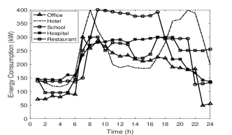
Figure 3: (a) A typical demand profile for different types of buildings (i.e., office, hotel, school, hospital, restaurant). (b) A typical wind and solar generation profile.

We set the ES roundtrip efficiency as $\eta^{\text{ch}},\eta^{\text{dis}}=0.9$. For the amortized ES capital price, we set the annual interest rate $r=0.06$ and the ES lifetime $L=10$ years. $|\Omega|=10$ representative scenarios are used to capture the volatility of renewable generation. The maximum trading power with the grid is set as $p^{g,\max}=1000$ $\mathrm{kW}$ for each building. The charging and discharging rate limits for each BC are set as $p^{\text{ch},\max},p^{\text{dis},\max}=500$\mathrm{kW}$$.

V-B RUS Price Model

We first empirically justify the quadratic price model, and then compare the RUS price with the projections of IES model.

To justify the quadratic price model, we first study the marginal ES capital investment w.r.t. the RUS for each BC with the IES model. We consider $N=5$ BCs of different types and set the grid price as $c^{\text{g+}}=0.3$s$$\mathrm{/}{\mathrm{k}\mathrm{W}\mathrm{h}}$ and $c^{\text{g-}}=0$. With IES model, the minimum ES capital cost of BC $i$ to achieve RUS $r_{i}$ can be obtained by solving the following problem:

$${Q}^{\scriptscriptstyle\text{IES}}_{i} (r_{i})=\min C_{\scriptscriptstyle E}E_{i}+C_{\scriptscriptstyle P}P_{i} \mathcal{P}_{\text{IES}}$$ ()

$$\text{subject~{}to}:$$

$$\quad 0\leq p^{\text{ch},\omega}_{i,t}\leq x^{\text{ch}}_{i,t}p^{\text{ch},\max},$$ (17a)

$$\quad 0\leq p^{\text{dis},\omega}_{i,t}\leq x^{\text{dis}}_{i,t}p^{\text{dis},\max},$$ (17b)

$$\quad e^{b,\omega}_{i,t+1}=e^{b,\omega}_{i,t}+p^{\text{ch},\omega}_{i,t}\eta^{\text{ch}}-p^{\text{dis},\omega}_{i,t}/\eta^{\text{dis}},$$ (17c)

$$\quad 0\leq e^{b,\omega}_{i,t}\leq E_{i},$$ (17d)

$$\quad p^{\text{ch},\omega}_{i,t},p^{\text{dis},\omega}_{i,t}\leq P_{i},$$ (17e)

$$\quad x^{\text{ch}}_{i,t}+x^{dis}_{i,t}\leq 1,x^{\text{ch}}_{i,t},x^{\text{dis}}_{i,t}\in\{0,1\},$$ (17f)

$$\quad p^{\text{ch},\omega}_{i,t}\leq p^{r,\omega}_{i,t},$$ (17g)

$$\quad p^{\text{g+},\omega}_{i,t}-p^{\text{g-},\omega}_{i,t}=p^{\text{ch},\omega}_{i,t}-p^{\text{dis},\omega}_{i,t}+p^{\text{d},\omega}_{i,t}-p^{\text{r},\omega}_{i,t},$$ (17h)

$$\quad x^{\text{g+},\omega}_{i,t}+x^{\text{g-},\omega}_{i,t}\leq 1,~{}x^{\text{g+},\omega}_{i,t},x^{\text{g-},\omega}_{i,t}\in\{0,1\},$$ (17i)

$$\quad p^{\text{g+},\omega}_{i,t}\leq x^{\text{g+},\omega}_{i,t}p^{g,\max},~{}p^{\text{g-},\omega}_{i,t}\leq x^{\text{g-},\omega}_{i,t}p^{g,\max},$$ (17j)

$$\quad\quad\quad~{}\forall\omega\in\Omega,\forall i\in\mathcal{N},t\in\mathcal{T}.$$

$$\quad C_{i}(\bm{y}^{\omega}_{i})\leq\overline{C}_{i}-(c^{\text{g+}}-c^{\text{g-}})r_{i},$$ (17k)

$$\text{var:}~{}E_{i},P_{i},y^{\omega}_{i},\forall\omega\in\Omega.$$

where problem ($\mathcal{P}_{\text{IES}}$) adopts the notations of Section III and the RUS $r_{i}$ can be regarded as an input.

For each BC (BC1-BC5), we can simulate their minimum ES capital cost w.r.t. the RUS $i$ by increasing $r_{i}$ from $r^{\min}_{i}=0$ to $r^{\max}_{i}$ with an incremental of $10$$\mathrm{kW}\text{\,}\mathrm{h}$. We display the simulated results in Fig. 4 (dotted curves). For each BC, we can find a quadratic function $\hat{Q}^{\scriptscriptstyle\text{IES}}_{i}(r_{i})=\hat{q}_{i}{r_{i}}^{2}$ that well fits the simulated curve (solid curves). This implies for the BCs with IES installations, the marginal ES capital cost w.r.t. the RUS can be approximately captured by a quadratic function. This somehow justifies the quadratic price model used by the ESO to charge the BCs for their requested RUS.

Figure 4: ES capital cost w.r.t the RUS $r_{i}$ for BC1-BC5 with IES model (dotted curve: simulated results. solid curves: fitted results).

Subsequently, we compare the optimal RUS price of CES model with the projections of IES model. For the IES model, the optimal RUS $\hat{r}_{i}$ and ES capital cost $\hat{Q}^{\scriptscriptstyle\text{IES}}_{i}(\hat{r}_{i})$ can be obtained from the simulations. For comparison, we can obtain the projected RUS price $\hat{q}_{i}=\hat{Q}^{\scriptscriptstyle\text{IES}}_{i}/{\hat{r}_{i}}^{2}$ for IES model. For the CES model, the optimal RUS $r^{*}_{i}$ and price $q^{*}_{i}$ are obtained by solving problem (${\cal P}$). For the two ES models, the optimal RUS and (projected) price are compared in TABLE I. We conclude the CES model provides a much lower RUS price to the BCs compared with IES model(i.e, $q^{*}_{i}<\hat{q}_{i}$) and enables higher renewable utilization (i.e., $r^{*}_{i}>\hat{r}_{i}$).

TABLE I: Optimal RUS and (projected) RUS price with the IES and CES model.

ES model	IES		CES
#BC	$\hat{r}_{i}$($\mathrm{kW}\text{\,}\mathrm{h}$)	$\hat{q}_{i}$($\times 10^{3}$ )	$r^{*}_{i}$($\mathrm{kW}\text{\,}\mathrm{h}$)	$q^{*}_{i}$($\times 10^{3}$ )
BC1	14.95	11.4	50.81	2.95
BC2	45.97	3.5	90.74	1.65
BC3	44.61	3.3	86.35	1.74
BC4	81.45	2.3	114.88	1.31
BC5	45.63	3.5	98.42	1.52

V-C ESO Profitability and Consumer Incentives

In this part, we study the ESO profitability and consumer incentives of the CES model. Particularly, we compare the CES model with i) an existing third-party based ES sharing model, referred to VES model [16, 13], and ii) IES model. For the VES model, the ESO charges the BCs by their required energy capacity (no charging and discharging rate limits) with a linear price model. The price is determined by the ESO to maximize its profit. We investigate a number of case studies under the different scales (i.e., $N\in\{5,10,15,20\}$ and grid price settings (i.e., $c^{\text{+}}_{g}=\{0.25,0.3,0.35\}$s$$\mathrm{/}{\mathrm{k}\mathrm{W}\mathrm{h}}$ and $c^{\text{-}}_{g}=0$ for all cases). Considering the problem complexity, we depend on simulations to obtain the equilibrium price for the VES model. Specifically, we simulate the ES rental price $q$ from $0.05$s$$\mathrm{/}{\mathrm{k}\mathrm{W}\mathrm{h}}$ to $0.5$ s$$\mathrm{/}{\mathrm{k}\mathrm{W}\mathrm{h}}$ with an incremental of $0.002$ s$$\mathrm{/}{\mathrm{k}\mathrm{W}\mathrm{h}}$. It’s clear that the equilibrium price corresponds to the point with maximal ESO profit if exists. For the CES model, the equilibrium price can be obtained by solving problem (${\cal P}$) based on CPLEX toolbox embedded in MATLAB. We compare the ESO profit with the VES and CES model under the different grid price settings in TABLE II. Firstly, we note the ESO profit is increasing w.r.t the scale and grid price both with the VES and CES model. While the former is straightforward, the latter can be understood that the BCs would require higher RUS under a higher grid price, thus creating higher profit for the ESO. Notably, the CES model can generate much higher ESO profit (i.e., about 2-4 times) than the VES model in the case studies.

TABLE II: ESO profit with VES and CES model.

N	$c^{\text{+}}_{g}=0.25$s$$\mathrm{/}{\mathrm{k}\mathrm{W}\mathrm{h}}$		$c^{\text{+}}_{g}=0.3$s$$\mathrm{/}{\mathrm{k}\mathrm{W}\mathrm{h}}$		$c^{\text{+}}_{g}=0.35$s$$\mathrm{/}{\mathrm{k}\mathrm{W}\mathrm{h}}$
	VES	CES	VES	CES	VES	CES
	(s$)	(s$)	(s$)	(s$)	(s$)	(s$)
5	3.22	23.83	8.57	34.45	15.54	29.56
10	25.74	73.83	47.96	100.09	67.54	102.83
15	37.66	116.89	70.41	157.17	91.79	179.34
20	54.47	191.23	102.75	251.63	130.64	271.90

Figure 5: Cost reduction for BC1-BC20 with different ES model (w/o ES model as benchmark) under the grid price settings: (a) $c^{\text{+}}_{g}=0.25s\$$$\mathrm{/}{\mathrm{k}\mathrm{W}\mathrm{h}}$, (b) $c^{\text{+}}_{g}=0.3s\$$$\mathrm{/}{\mathrm{k}\mathrm{W}\mathrm{h}}$, (c) $c^{\text{+}}_{g}=0.35s\$$$\mathrm{/}{\mathrm{k}\mathrm{W}\mathrm{h}}$.

Further, we look into the consumer incentives with the different ES models. For comparisons, we use each BC’s electricity bill without ES (w/o ES) as its baseline and refer to the cost reduction over the baseline as consumer incentive. We compare the CES model with the IES and VES model. For the IES model, each BC installs individual ES to support local renewable utilization so as to minimize its total cost. For display limits, we use the case with $N=20$ BCs as an example and show the consumer incentives with the different ES models in Fig. 5 (we can observe the similar results for the other scales. First, we see the VES model provides the least cost reduction to the BCs for all grid price settings. Therefore, we can envision the BCs would prefer to install individual ES rather than participate in the VES model considering the economic gains alone. In contrast, the CES model yields the most cost reduction for each BC over the other ES models. Further, we can observe some interesting phenomenon from the low to high grid price settings. For the IES model, the cost reduction for each BC increases w.r.t. the grid price. Particularly, for the high grid price, i.e., $c^{\text{+}}_{g}=0.35s\$$\mathrm{kW}\text{\,}\mathrm{h}$$, the IES model can provide comparable cost reduction to most BCs (i.e., BC2-BC4, BC6-BC7, BC10-BC11, BC16-BC20) compared with the CES model. This implies the economic gap between the IES and CES model will diminish with the increase of grid price. This is reasonable that the economic barriers of IES model cased by the ES capital cost will drop when the grid price increase. We can also interpret the results from the opposite that the difference over the different ES models will vanish if the ES capital cost is brought down to some boundaries.

V-D Social welfare and ES efficiency

We study the social welfare and ES efficiency with the CES model under the different scale (i.e, $N=\{5,10,15,20\}$) and grid price (i.e., $c^{\text{+}}_{g}=\{0.25,0.3,0.35\}$s$$\mathrm{/}{\mathrm{k}\mathrm{W}\mathrm{h}}$ and $c^{\text{-}}_{g}=0$) settings. We compare the CES model with the IES and VES model and use the w/o ES and CEMS model as the references of lowest and highest social welfare.

For the CES and VES model, the social welfare is characterized by the total cost of all BCs minus the profit of ESO. For the IES and CMES model, the social welfare equals to the total electricity bills of all BCs plus the ES capital cost. For the w/o ES model, the social welfare defines the total electricity bills of all BCs as there is no ES installed.

TABLE III: Social welfare of different ES models.

(a) grid price $c^{\text{+}}_{g}=0.25s\$$$\mathrm{/}{\mathrm{k}\mathrm{W}\mathrm{h}}$

N	ES models
	w/o ES	IES	VES	CES	CMES
	($\times 10^{2}$s$)	($\times 10^{2}$s$)	($\times 10^{2}$s$)	($\times 10^{2}$s$)	($\times 10^{2}$s$)
5	10.73	10.65	10.70	10.02	9.90
10	23.62	23.42	23.22	21.67	21.40
15	35.60	35.37	35.05	32.49	32.30
20	47.19	46.77	46.36	42.31	42.08

(b) grid price $c^{\text{+}}_{g}=0.3s\$$$\mathrm{/}{\mathrm{k}\mathrm{W}\mathrm{h}}$

N	ES models
	w/o ES	IES	VES	CES	CMES
	($\times 10^{2}$s$)	($\times 10^{2}$s$)	($\times 10^{2}$s$)	($\times 10^{2}$s$)	($\times 10^{2}$s$)
5	12.88	12.70	12.68	11.88	11.78
10	28.34	27.92	27.57	25.66	25.48
15	42.72	42.21	41.64	38.66	38.53
20	56.63	55.74	54.99	50.46	50.15

(b) grid price $c^{\text{+}}_{g}=0.35s\$$$\mathrm{/}{\mathrm{k}\mathrm{W}\mathrm{h}}$

N	ES models
	w/o ES	IES	VES	CES	CMES
	($\times 10^{2}$s$)	($\times 10^{2}$s$)	($\times 10^{2}$s$)	($\times 10^{2}$s$)	($\times 10^{2}$s$)
5	15.03	14.71	14.73	13.64	13.63
10	33.06	32.34	31.93	29.54	29.54
15	49.84	48.95	48.32	44.76	44.73
20	66.07	64.56	64.03	58.23	58.19

We report the social welfare of different cases in TABLE III. First of all, the w/o ES and CMES model provide the lowest and highest social welfare for each case as anticipated. Obviously, the CES model outperforms the IES and VES model in social welfare as the former provides lower social cost over the other two for each case. Besides, we see the VES and IES model are comparable in social cost for each case.

Further, to quantify the social performance gaps of different ES models, we define a relative social cost (RSC) metric that captures the normalized social performance of different ES models over the CMES and w/o ES model, i.e.,

$$\text{RSC}(x)=\frac{\text{SC}(x)-\text{SC}(\text{CMES})}{\text{SC}(\text{w/o ES})-\text{SC}(\text{CMES})}$$

where $x$ denotes an ES model, i.e., $x\in\{\text{IES},\text{VES},\text{CES}\}$. Intuitively, we have $\text{RSC}(\text{CMES})=0$ (social optima) and $\text{RSC}(\text{w/o ES})=1$. Besides, we note the smaller the RSC, the higher of social welfare. For comparisons, we visualize the RSC metric of different ES models under the different scale (i.e., $N\in\{5,10,15,20\}$) and grid price (i.e., $c^{\text{+}}_{g}=\{0.25,0.3,0.35\}$s$$\mathrm{/}{\mathrm{k}\mathrm{W}\mathrm{h}}$) settings in Fig. 6. Firstly, we see the RSC of all ES models (i.e., IES, VES, CES) are bounded by the w/o ES and CMES model (i.e., $\text{RSC}(\text{IES}),\text{RSC}(\text{VES}),\text{RSC}(\text{CES})\in[0,1]$). Besides, the IES and VES only achieve minor social superiority over the lower baseline ( i.e., RSC(w/o ES) =0) for all cases. Nevertheless, the CES model dominates the IES and VES model for all case in social welfare (i.e., $\text{RSC}(\text{CES})\ll\text{RSC}(\text{IES}),\text{RSC}(\text{VES}$) ). More notably, we see the CES model achieves the near social optima (i.e., $\text{RSC}(\text{CES})\approx 1$).

Figure 6: Relative social cost (RSC) of different models (w/o ES and CMES as benchmarks: RSC(w/o ES) = 0 and RSC(CMES) = 1) under the grid price settings (a) $c^{\text{+}}_{g}=0.25s\$$$\mathrm{/}{\mathrm{k}\mathrm{W}\mathrm{h}}$, (b) $c^{\text{+}}_{g}=0.3s\$$$\mathrm{/}{\mathrm{k}\mathrm{W}\mathrm{h}}$. (c) $c^{\text{+}}_{g}=0.35s\$$$\mathrm{/}{\mathrm{k}\mathrm{W}\mathrm{h}}$.

The high social welfare generally corresponds to high resource efficiency. To further demonstrate it, we study the ES efficiency with the CES model by comparing with the VES model. Specifically, we study the ES utilization indicated by the State-of-Charge (SoC) and charging/discharging rates over the contracted time period. We use the case with $N=10$ BCs and grid price $c^{\text{+}}_{g}=0.35s\$$$\mathrm{/}{\mathrm{k}\mathrm{W}\mathrm{h}}$ for a randomly picked scenario as an example (similar results are observe in the other cases). The charging/discharging rates ($\mathrm{kW}$) and the SoC (%) for the BCs (BC1-BC10) with the two ES models are contrasted in Fig. 7 and Fig. 8, respectively. Notably, we see CES model exhibits much higher ES utilization than the VES model both for energy capacity (i.e., SoC) and power capacity (i.e., charging and discharging rates). Moreover, we can observe some interesting phenomenon regarding the ES operation patterns over the two ES models. Specifically, from Fig. 7, we observe the BCs mostly charge or discharge synchronously and do not see much cancellations in sharing with the VES model as expected in [16, 13]. This can be understood that though the ESO expects the BCs to charge and discharge in a complementary manner, the linear price model based on energy capacity does not provide the coordination signals. In other words, the BCs operate their contracted energy capacity separately, resulting in the low utilization of ES resources, especially the power capacity. Actually, this leads to the short profitability of ESO as discussed in Section V-C. Nevertheless, we can observe quite different results for the CES model. At each instant, we can see both charging and discharging from different BCs, resulting in frequent cancellation and high ES utilization both for the energy and power capacity. This demonstrates the favorable performance of the CES model in shaping ES efficiency.

Figure 7: Charging/discharging rates of BC1-BC10 with (a) VES model, and (b) CES model.

Figure 8: State-of-charge (SoC) of BC1-BC10 with (a) VES model, and (b) CES model.

VI Conclusion

This paper proposed a cloud energy storage (CES) model for enabling distributed renewable integration of building consumers (BCs). Different from most existing ES sharing models that the entity gains profit by leasing energy or power capacity, our CES model is deployed by allowing the energy storage operator (ESO) to sell renewable utilization service (RUS) to its consumers. To capture the increasing marginal “effort” (i.e., ES resources) made by the ESO to achieve the requested RUS, we adopted a quadratic price model which was empirically justified through simulations. We formulated the interactions between the ESO and the BCs as a Stackelberg game and demonstrated the existence of an equilibrium. Besides, we showed the CES model can achieve better social welfare than individual ES (IES) model. The superior performance of the CES model over the IES model and an existing ES sharing model (referred to VES model) are also demonstrated via case studies. Specifically, we showed the CES model can provide 2-4 times ESO profit over the VES model. Meanwhile, higher cost reduction are provided to the BCs. Last and noteworthy, we showed the CES model can achieve near social optima and high ES efficiency (i.e., utilization) which are not provided by the other ES sharing models. Conclusively, this paper can work as an example to show how market design and sharing economy can shape the efficiency of energy systems.

References

- [1] S. Weitemeyer, D. Kleinhans, T. Vogt, and C. Agert, “Integration of renewable energy sources in future power systems: The role of storage,” Renewable Energy, vol. 75, pp. 14–20, 2015.
- [2] “Openei.” https://www.irena.org/-/media/Files/IRENA/Agency/Publication/2020/Mar/IRENA_RE_Capacity_Highlights_2020.pdf. Accessed: 2020-10-13.
- [3] “Openei.” https://www.greentechmedia.com/articles/read/bloombergnef-solar-and-wind-add-two-thirds-of-new-generation-in-20. Accessed: 2020-10-13.
- [4] D. Stenclik, P. Denholm, and B. Chalamala, “Maintaining balance: the increasing role of energy storage for renewable integration,” IEEE Power and Energy Magazine, vol. 15, no. 6, pp. 31–39, 2017.
- [5] C. Goebel and H.-A. Jacobsen, “Bringing distributed energy storage to market,” IEEE Transactions on Power Systems, vol. 31, no. 1, pp. 173–186, 2015.
- [6] M. Arbabzadeh, R. Sioshansi, J. X. Johnson, and G. A. Keoleian, “The role of energy storage in deep decarbonization of electricity production,” Nature communications, vol. 10, no. 1, pp. 1–11, 2019.
- [7] U. EIA, “Levelized cost and levelized avoided cost of new generation resources in the annual energy outlook 2016,” Washington DC, USA, 2016.
- [8] M. S. Ziegler, J. M. Mueller, G. D. Pereira, J. Song, M. Ferrara, Y.-M. Chiang, and J. E. Trancik, “Storage requirements and costs of shaping renewable energy toward grid decarbonization,” Joule, vol. 3, no. 9, pp. 2134–2153, 2019.
- [9] K. Barron, E. Kung, and D. Proserpio, “The sharing economy and housing affordability: Evidence from airbnb.,” in EC, p. 5, 2018.
- [10] N. Agatz, A. Erera, M. Savelsbergh, and X. Wang, “Optimization for dynamic ride-sharing: A review,” European Journal of Operational Research, vol. 223, no. 2, pp. 295–303, 2012.
- [11] P. Lombardi and F. Schwabe, “Sharing economy as a new business model for energy storage systems,” Applied energy, vol. 188, pp. 485–496, 2017.
- [12] P. Chakraborty, E. Baeyens, K. Poolla, P. P. Khargonekar, and P. Varaiya, “Sharing storage in a smart grid: A coalitional game approach,” IEEE Transactions on Smart Grid, vol. 10, no. 4, pp. 4379–4390, 2018.
- [13] D. Zhao, H. Wang, J. Huang, and X. Lin, “Virtual energy storage sharing and capacity allocation,” IEEE Transactions on Smart Grid, vol. 11, no. 2, pp. 1112–1123, 2019.
- [14] J. Liu, N. Zhang, C. Kang, D. S. Kirschen, and Q. Xia, “Decision-making models for the participants in cloud energy storage,” IEEE Transactions on Smart Grid, vol. 9, no. 6, pp. 5512–5521, 2017.
- [15] Z. Liu, J. Yang, W. Song, N. Xue, S. Li, and M. Fang, “Research on cloud energy storage service in residential microgrids,” IET Renewable Power Generation, vol. 13, no. 16, pp. 3097–3105, 2019.
- [16] D. Zhao, H. Wang, J. Huang, and X. Lin, “Pricing-based energy storage sharing and virtual capacity allocation,” in 2017 IEEE International Conference on Communications (ICC), pp. 1–6, IEEE, 2017.
- [17] H. He, L. Cheng, H. Zhu, L. Tang, E. Du, and C. Kang, “Optimal capacity pricing and sizing approach of cloud energy storage: A bi-level model,” in 2019 IEEE Power & Energy Society General Meeting (PESGM), pp. 1–5, IEEE, 2019.
- [18] Z. Mi and D. Coffman, “The sharing economy promotes sustainable societies,” Nature communications, vol. 10, no. 1, pp. 1–3, 2019.
- [19] W. Zhong, K. Xie, Y. Liu, C. Yang, S. Xie, and Y. Zhang, “Online control and near-optimal algorithm for energy storage sharing in smart grid,” in ICC 2019-2019 IEEE International Conference on Communications (ICC), pp. 1–6, IEEE, 2019.
- [20] W. Tushar, B. Chai, C. Yuen, S. Huang, D. B. Smith, H. V. Poor, and Z. Yang, “Energy storage sharing in smart grid: A modified auction-based approach,” IEEE Transactions on Smart Grid, vol. 7, no. 3, pp. 1462–1475, 2016.
- [21] J. Yao and P. Venkitasubramaniam, “Stochastic games of end-user energy storage sharing,” in 2016 IEEE 55th Conference on Decision and Control (CDC), pp. 4965–4972, IEEE, 2016.
- [22] J. Yao and P. Venkitasubramaniam, “Privacy aware stochastic games for distributed end-user energy storage sharing,” IEEE Transactions on Signal and Information Processing over Networks, vol. 4, no. 1, pp. 82–95, 2017.
- [23] H. Zhu and K. Ouahada, “Credit-based distributed real-time energy storage sharing management,” IEEE Access, vol. 7, pp. 185821–185838, 2019.
- [24] N. Vespermann, T. Hamacher, and J. Kazempour, “Access economy for storage in energy communities,” IEEE Transactions on Power Systems, 2020.
- [25] Y. Dvorkin, R. Fernandez-Blanco, D. S. Kirschen, H. Pandžić, J.-P. Watson, and C. A. Silva-Monroy, “Ensuring profitability of energy storage,” IEEE Transactions on Power Systems, vol. 32, no. 1, pp. 611–623, 2016.
- [26] H. Pandžić, “Optimal battery energy storage investment in buildings,” Energy and Buildings, vol. 175, pp. 189–198, 2018.
- [27] Y. Yang, G. Hu, and C. J. Spanos, “Optimal sharing and and fair cost allocation of community energy storage,” arXiv preprint arXiv:2010.15455, 2020.
- [28] “Openei.” https://openei.org/datasets/files/961/pub/. Accessed: 2020-08-05.
- [29] “Measurement and instrumentation data center (midc), nrel transforming energy.” https://midcdmz.nrel.gov/apps/daily.pl?site=NWTC&start=20010824&yr=2020&mo=1&dy=28. Accessed: 2020-08-05.