Deferrable Load Scheduling under Demand Charge: A Block Model-Predictive Control Approach

Abstract

Optimal scheduling of deferrable electrical loads can reshape the aggregated load profile to achieve higher operational efficiency and reliability. This paper studies deferrable load scheduling under demand charge that imposes a penalty on the peak consumption over a billing period. Such a terminal cost poses challenges in real-time scheduling when demand forecasts are inaccurate. A block model-predictive control approach is proposed by breaking the demand charge into a sequence of stage costs. The problem of charging electric vehicles is used to illustrate the efficacy of the proposed approach. Numerical examples show that the block model-predictive control outperforms the benchmark methods in various settings.

I Introduction

The scheduling of deferrable loads has shown promising benefits to many distribution system applications, such as flexible load aggregation [1, 2, 3, 4], serving electric vehicle (EV) charging demands [5, 6, 7, 8, 9, 10, 11, 12], and data center power management [13]. The possibility of “load shifting” enables the optimal shaping of demand patterns, improving power system flexibility, and achieving enhanced economic goals.

For commercial and industrial consumers, a significant challenge in real-time scheduling of deferrable loads is that the demand charge imposed on the maximum consumption over a billing period can be a substantial part of the overall operating cost. Because demand charge is a terminal cost at the end of the billing period, a scheduling decision policy needs to consider the impact of the past and current decisions on the overall peak consumption. Without accurate demand forecasts, deferring current demands to the future may incur substantial demand charge when the deferred demands compete with new demand arrivals for services. The problem becomes even more challenging when demands have completion deadlines with penalties on unmet demands.

We study the real-time deferrable load scheduling under demand charge (DLS-DC), where stochastic demands arrive with random energy and service completion requests. Practical examples of DLS-DC include scheduling EV charging in public charging facilities and cloud services in large data centers. In both cases, the demand volume during peak hours could make the demand charge substantial for a service provider.

I-A Related Work

The scheduling of deferrable loads has drawn much attention over the past few decades. A popular theme is to formulate the problem as a dynamic program (DP) for real-time control. To overcome DP’s curse of dimensionality, index policies and priority rules have been proposed in [14, 10, 15]. In particular, for the large scale EV charging with stochastic demands and random arrivals, the Whittle’s index policy was developed in [14] and shown to be symptomatically optimal in the light traffic regimes. In [10], Xu et al. established a partial priority rule that prioritized EVs with Less Laxity and Longer remaining Processing time (LLLP). This result was further extended by Jin and Xu in [15], who proposed a complete scheduling rule that prioritized EVs under Less Laxity first with Later Deadline (LLF-LD).

Deterministic deadline scheduling policies such as Earliest Deadline First (EDF) [16] and Least Laxity First (LLF) [17] have also been considered for deferrable load scheduling. These techniques are optimal regardless of the underlying stochastic models under restricted conditions. In general, such techniques are suboptimal in either robust or average measures, although finite competitive ratio scheduling exists for some cases [5].

Model-predictive control (MPC) has been widely adopted for online scheduling strategies for its simplicity and favorable performance in many applications. In the absence of demand charge, MPC has been applied for the real-time scheduling of deferrable loads [4], including cases involving random arrivals of demands [11] and random network topology changes [12]. MPC can also be utilized for tracking a given pre-scheduled trajectory [18, 3]. Chen et al. [3] showed that the distribution of tracking errors would concentrate around if forecasting errors were bounded.

Demand charge has been in place in the U.S. since the 1900s [19], and it has been applied to EV charging [11], thermostatic control of commercial buildings [20, 21], and data centers [22, 13]. In [23], Kumar et al. proposed a stochastic MPC approach to schedule stationary batteries that simultaneously served local demands and provided frequency regulation services. Most relevant to this paper, perhaps, are the work of Jin and Xu [15, 24] and that by Risbeck and Rawllings in [25]. In [15], Jin and Xu proposed a priority rule for real-time scheduling of EV charging that had strong performance guarantee, although demand charge was not considered. Demand charge was considered explicitly in [24] for the scheduling of non-deferrable loads by tracking the up-to-date peak power in a DP framework. In [25], the authors proposed the so-called economic MPC (EMPC) with a special terminal cost and constraint to track a specific reference trajectory. In the absence of such a reference, the EMPC formulation in [25] does not apply directly.

I-B Summary of Results

Formulating DLS-DC as a stochastic optimal control problem, we propose a block model-predictive control (BMPC) approach by tracking the peak consumption and assessing the impact of the demand charge in each stage. Whereas the idea of tracking the peak consumption was considered in [13, 24, 25], BMPC differs from existing techniques in the specific stage costs used in the optimization, and how the peak consumption is tracked over multiple scheduling intervals.

There are apparent similarities between BMPC and EMPC [25]; both are derived based on the principle of MPC, and both involve some forms of terminal costs. The main difference is that EMPC solves a deterministic optimization problem aimed to track a reference trajectory. Thus the performance of EMPC depends on the quality of such a reference. BMPC, on the other hand, solves a stochastic one with exogenous random parameters, which does not require a reference trajectory but exploits generically short-term forecasts in a rolling-window fashion. The terminal costs used in the two approaches are, therefore, quite different. Another non-trivial difference is that EMPC assumes that the measurement window in which the maximum consumption is measured matches the scheduling interval. Typically in practice, a demand charge is levied on the maximum average consumption within several scheduling intervals.

We conduct numerical simulations to compare BMPC with four state-of-the-art algorithms including nominal MPC (NMPC) without demand charge, EMPC[25], EDF [16] and LLF-LD[15]. Numerical results demonstrate that BMPC achieves near-optimal performance in most cases. In particular, BMPC can achieve 10% more total reward than the second best approach when EV charging requests are stochastic. Comparing with EDF and LLF-LD, BMPC can obtain more than 20% total reward on average.

The remainder of this paper is organized as follows. We formulate the DLS-DC problem as a stochastic optimal control problem in Section II. In Section III, we develope the BMPC algorithm and present justifications on the terminal cost for the demand charge. In Section IV, an application study on EV charging scheduling is presented. Then we demonstrate the numerical results in Section V. Finally, we conclude the paper in Section VI.

II DLS-DC Model

We present in this section a general stochastic control formulation of DLS-DC. Deferrable loads are flexible demands such that their services can be delayed. By shifting part or all of the demands, DLS-DC has strong inter-temporal dependencies. In Section IV, we consider EV charging as a specific form of deferrable loads.

We model the process of scheduling of deferrable loads by a discrete-time dynamic equation

$$x_{t+1}=f_{t}(x_{t},u_{t},\xi_{t}),~{}t\in\mathcal{T}=\{0,1,\cdots,T-1\},$$ (1)

where the time index $t$ models the decision interval (or stage), $x_{t}$ the state vector of deferrable loads that includes the amount of unserved demands, $u_{t}$ the control vector such as the demands to be served in interval $t$, and $\xi_{t}$ the exogenous random parameter (such as new arrivals of demands) that influences the state of the deferrable loads in the next stage.

We consider the problem of optimal DLS-DC by a sequence of control laws $\{\mu_{t}\}_{t=0}^{T-1}$, where $\mu_{t}$ maps the state of deferrable loads $x_{t}$ and the exogenous input $\xi_{t}$ to the control $u_{t}=\mu_{t}(x_{t},\xi_{t})$ at stage $t$. The objective is to maximize the expected total reward of scheduling under demand charge defined by the following stochastic optimal control problem (2):

$$\max_{\{\mu_{t}\}_{t\in\mathcal{T}}}~{} \mathbb{E}\left[\sum_{t\in\mathcal{T}}{\mathcal{G}_{t}(\tilde{x}_{t},\tilde{u}_{t},\xi_{t})}-\mathcal{C}(\psi)\right]$$ (2a)

s.t. $$\tilde{x}_{t+1}=f_{t}(\tilde{x}_{t},\tilde{u}_{t},\xi_{t}),\quad t\in\mathcal{T},$$ (2b)

$$h_{t}(\tilde{x}_{t},\tilde{u}_{t},\xi_{t})\leq 0,\quad t\in\mathcal{T},$$ (2c)

$$\tilde{u}_{t}=\mu_{t}(\tilde{x}_{t},\xi_{t}),\quad t\in\mathcal{T},$$ (2d)

$$\psi=\max_{t\in\{0,\ell,2\ell,\dots,T-\ell\}}~{}\left\{\frac{1}{\ell}\sum_{\tau=t}^{t+\ell-1}{c(\tilde{x}_{\tau},\tilde{u}_{\tau},\xi_{\tau})}\right\},$$ (2e)

$$\text{initializing}~{}\tilde{x}_{0}=x_{0},$$ (2f)

where $\tilde{x}_{t}$ and $\tilde{u}_{t}$ are decision variables corresponding to the state and control at stage $t$ respectively, $\mathcal{G}_{t}(\cdot)$ the stage reward function, representing the reward of action of serving demands at stage $t$, $h_{t}(\cdot)$ a set of constraints on the state and control (e.g. maximum power drawn from the grid), $c(\tilde{x}_{t},\tilde{u}_{t},\xi_{t})$ the total demands served in interval $t$, $\psi$ the maximum average demand in non-(overlapping) $\ell$ consecutive scheduling intervals that are referred to as (average-power) measurement window, and $\mathcal{C}(\psi)$ the terminal cost that models the demand charge. Note that the model defined in (2) is applicable to a much broader class of scheduling problems beyond DLS-DC.

Figure 1: Temporal structure of BMPC and NMPC with an example of $W=2\ell$.

The main difficulties of dealing with demand charges in the stochastic optimal control framework come from the mismatch of different timescales. In particular, three timescales coexist in the formulated DLS-DC model:

1. the control $u_{t}=\mu_{t}(x_{t},\xi_{t})$ happens at every stage $t\in\mathcal{T}=\{0,1,\cdots,T-1\}$;

2. the peak average consumption that sets the demand charge is calculated at the end of each measurement window at $t=\{\ell,2\ell,\cdots,T\}$;

3. the demand charge is imposed at the terminal stage $T$.

Because a stage reward $\mathcal{G}_{t}(x_{t},u_{t},\xi_{t})$ is realized at every stage $t$ whereas the demand charge $\mathcal{C}(\psi)$ is levied at the end of the entire control horizon, it is challenging to balance the trade-off between the immediate stage reward and the uncertain demand charge set at the end of the scheduling horizon.

III Block Model Predictive Control

This section formalizes a block decision structure and proposes an MPC-based framework for DLS-DC. The proposed framework is termed Block MPC because the rolling window moves a block of $\ell$ stages at a time.

III-A Block Model-Predictive Control under Demand Charge

To address the timescale mismatch issues (see Section II) arising from the demand charge, we introduce an additional system state $\phi_{t}$ at every stage $t$, which tracks the highest average consumption over an $\ell$-sized measurement window until stage $t$. The new state variable $\phi_{t}$ evolves according to

$$\phi_{t+1}=\begin{cases}\max\left\{\phi_{t},\frac{\sum_{\tau=t-\ell+1}^{t}{c(x_{\tau},u_{\tau},\xi_{\tau})}}{\ell}\right\}&\text{if}~{}t+1\in\mathcal{T^{\prime}},\\ \phi_{t}&\text{otherwise},\end{cases}$$ (3)

where $\mathcal{T^{\prime}}=\{0,\ell,2\ell,\dots,T-\ell\}$ denotes the set of the beginnings of each measurement window. Note that $\phi_{t+1}\geq\phi_{t}$ for every $t\in\mathcal{T}$. Therefore, the optimal DLS-DC (2) can be equivalently formulated as:

$$\max_{\{\mu_{t}\}_{t\in\mathcal{T}}}{} \mathbb{E}\left[\sum_{t\in\mathcal{T}}{\mathcal{G}_{t}(\tilde{x}_{t},\tilde{u}_{t},\xi_{t})}-\mathcal{C}(\tilde{\phi}_{T})\right]$$ (4)

s.t. $$\eqref{eqn:sys_state}\eqref{eqn:sys_cons}\eqref{eqn:sys_control}\eqref{eqn:sys_1}\eqref{eqn:new_state_update},$$

$$\text{initializing}~{}\tilde{\phi}_{0}=\phi_{0},$$

where $\tilde{\phi}_{t}$ denotes the decision variable corresponding to the new state at stage $t$. With the new state variable, it is much easier to apply the idea of MPC on the reformulated problem (4). Generally, MPC considers the optimal control problem of a shorter control horizon $\{t,\cdots,t+W\}$ and utilizes a forecasted trajectory $\{\hat{\xi}_{k}\}_{k=t}^{t+W-1}$. As a result, BMPC solves the following optimal control problem for a rolling window of length $W$ at $t\in\mathcal{T^{\prime}}$:

$$\max_{\{\tilde{u}_{k}\}_{k=t}^{t+W-1}}~{} \sum_{k=t}^{t+W-1}\mathcal{G}_{k}\big{(}\tilde{x}_{k},\tilde{u}_{k},\hat{\xi}_{k}\big{)}-\mathcal{H}(\tilde{\phi}_{t+W})$$ (5a)

s.t. $$\tilde{x}_{k+1}=f_{t}(\tilde{x}_{k},\tilde{u}_{k},\hat{\xi}_{k}),$$ (5b)

$$\tilde{\phi}_{k}~{}\text{updates as in}~{}\eqref{eqn:new_state_update},$$ (5c)

$$h_{t}(\tilde{x}_{k},\tilde{u}_{k},\hat{\xi}_{k})\leq 0,$$ (5d)

$$\hskip 85.35826ptk=t,\dots,t+W-1,$$

$$\text{initializing}~{}\tilde{x}_{t}=x_{t},\tilde{\phi}_{t}=\phi_{t},$$ (5e)

where $\mathcal{H}(\tilde{\phi}_{t+W})$ is the BMPC terminal cost (to be specified in Section III-B). The main difference between BMPC and the nominal MPC (NMPC) (see Section III-C) is the block structure, illustrated in Fig. 1. Instead of moving from stage $t$ to $t+1$, BMPC moves one block ($\ell$ stages) each time, i.e., from $t$ to $t+\ell$. The optimal controls of (5) in the first block $\{\tilde{u}^{*}_{t},\cdots,\tilde{u}^{*}_{t+\ell-1}\}$ will be implemented. Others $\{\tilde{u}^{*}_{t+\ell},\cdots,\tilde{u}^{*}_{t+W-1}\}$ are only advisory.

The BMPC approach is summarized as Algorithm 1 below. Two factors affect the performance of BMPC: an initial guess on the maximum average consumption $\phi_{0}$, and a terminal cost $\mathcal{H}(\phi_{t+W})$. An accurate estimate on $\phi_{0}$ can be obtained using external information, e.g., learning from historical data. The choice of the terminal cost $\mathcal{H}(\phi_{t+W})$ lies at the heart of BMPC solution to DLS-DC. Detailed discussions and comparisons are in Section III-B.

1:  Initialization: Initialize system with $x_{0}$, $\phi_{0}$, $W$ and $\ell$.

2:  for $t\in\{0,\ell,\cdots,T-\ell\}$ do

3:     Observe the system current state $x_{t}$, the up-to-date highest average consumption $\phi_{t}$ and the actual input $\xi_{t}$;

4:     Forecast the random inputs $\{\hat{\xi}_{k}\}_{k=t+1}^{t+W-1}$ over stage $t+1$ to $t+W-1$;

5:     Solve the BMPC Problem (5);

$$\{u_{k}\}_{k=t}^{k+W-1}=\text{BMPC}(x_{t},\phi_{t},\{\hat{\xi}_{k}\}_{k=t}^{t+W-1})$$ (6)

6:     Take the the first $\ell$-stage controls from the solution to (5): $\bm{U}_{t}^{*}=(u^{*}_{t},\dots,u^{*}_{t+\ell-1})$;

7:     for $j\in\{t,t+1,\dots,t+\ell-1\}$ do

8:        Observe system state $x_{j}$ and the actual input $\xi_{j}$;

9:        Take $u^{*}_{j}=\mu_{j}(x_{j},\xi_{j})$ and update system state to $x_{j+1}$ according to (1);

10:        Update $\phi_{t}$ according to (3). 

11:     end for

12:  end for

Algorithm 1 BMPC under Demand Charge

III-B BMPC Terminal Cost $\mathcal{H}(\phi_{t+W})$

Intuitively, good choices of the terminal cost $\mathcal{H}(\phi_{t+W})$ should reflect the amortization of the demand charge in the current operating interval $t$. Some primitive forms of the terminal cost could be:

$$\mathcal{H}(\phi_{t+W}):=\mathcal{C}(\phi_{t+W}),\quad t\in\mathcal{T^{\prime}},$$ (7a)

$$\mathcal{H}(\phi_{t+W}):=\frac{W}{T}\mathcal{C}(\phi_{t+W}),\quad t\in\mathcal{T^{\prime}}.$$ (7b)

However, these two choices perform poorly in practice because (7a) imposes the demand charge over the entire control horizon $T$ on the rolling window. When $W\ll T$, the demand charge $\mathcal{C}(\phi_{t+W})$ would dominate the total stage reward of the rolling window. As a result, the solution in this setting will often be so conservative that schedulers would rather sacrifice most of the stage reward than incur a large demand charge cost. In addition, (7a) fails to capture the fact that the demand charge is only posed for the peak consumption.

A slightly better choice is (7b), which splits the demand charge equally among $T$ stages. This choice essentially assumes that the states of deferrable loads within each measurement window are almost identical, which is often not true in practice.

We propose a more judicious choice

$$\mathcal{H}(\phi_{t+W}):=\mathcal{C}(\phi_{t+W}-\phi_{t}),~{}t\in\mathcal{T^{\prime}}.$$ (8)

The rationale behind (8) is twofold. First, it is clear that $\phi_{t+W}\geq\phi_{t}$ always holds true according to (3). If the peak consumption of the current rolling window $\{t,\cdots,t+W\}$ is no higher than the previous one ($\phi_{t+W}=\phi_{t}$), no additional cost should be considered, i.e., $\mathcal{H}(\phi_{t+W})=0$. Additional cost occurs only when the peak consumption increases, i.e., $\phi_{t+W}>\phi_{t}$.

The BMPC terminal cost can be further justified for power system applications where the demand charge cost is linear. In this case, we have

$$\mathcal{C}(\phi_{T})=\mathcal{C}(\phi_{0})+\sum_{t\in\mathcal{T^{\prime}}}\mathcal{H}(\phi_{t+W})=\mathcal{C}(\phi_{0})+\sum_{t\in\mathcal{T}}\mathcal{C}(\phi_{k+1}-\phi_{k}),$$ (9)

which enables us to define a revised stage reward function that considers the cost of the demand charge at each stage $t\in\mathcal{T}$:

$$\mathcal{V}_{t}(x_{t},u_{t},\xi_{t},\phi_{t}):=\mathcal{G}_{t}(x_{t},u_{t},\xi_{t})-\mathcal{C}(\phi_{t+1}-\phi_{t}).$$ (10)

It is clear that (8) is a direct result of formulating BMPC using (10). The equation above reveals that (8) embeds the demand charge cost, which occurs at the end of control horizon, into each stage as decomposed in (10). Therefore, (8) effectively avoids the inferior performance by directly using the demand charge structure such as (7a) or (7b).

III-C Related MPC Approaches

We summarize two related MPC approaches as benchmarks in our comparison studies. The first is the nominal MPC without demand charge, where no demand charge penalty is added to the objective. The second is a modification of EMPC [25] so that it applicable for general measurement window size $\ell$.

III-C1 Nominal MPC (NMPC) without Demand Charge

Instead of moving $\ell$ steps every time as in the BMPC approach, NMPC moves only one step at each time (see Fig. 1), i.e., solving the following optimization problem consisting of $W$ stages at every stage $t\in\mathcal{T}$:

$$\max~{}J_{t}^{\text{NMPC}} :=\sum_{k=t}^{t+W-1}{\mathcal{G}(\tilde{x}_{k},\tilde{u}_{k},\hat{\xi}_{k})}$$ (11)

s.t. $$\eqref{eqn:bmpc_sys}\eqref{eqn:bmpc_cons},$$

$$\text{initializing}~{}\tilde{x}_{t}=x_{t}.$$

Unlike BMPC, only the optimal control $\tilde{u}^{*}_{t}$ will be implemented. Others $\{\tilde{u}^{*}_{t+1},\cdots,\tilde{u}^{*}_{t+W-1}\}$ are only advisory. Note that NMPC does not take the demand charge into consideration, which is another major difference from BMPC.

III-C2 Economic MPC (EMPC) [25]

Here we demonstrate the formulation of EMPC under DLS-DC when $\ell=1$ and then present a slight modification of EMPC so that it applies to cases when $\ell\geq 2$.

Let $(\mathbf{x}^{\text{ref}},\mathbf{u}^{\text{ref}},\bm{\xi}^{\text{ref}})$ be an arbitrarily known reference trajectory over $\mathcal{T}$. For each $t\in\mathcal{T}$, the objective of EMPC is defined as

$$J^{\text{EMPC}}_{t}:=\sum_{k=t}^{t+W-1} {\mathcal{G}_{k}(x_{k},u_{k},\xi_{k}^{\text{ref}})}$$ (12)

$$-\mathcal{C}(\max(\phi_{t+W},\breve{\psi}_{t+W}^{\text{ref}}))-\mathcal{C}(\psi^{\text{ref}}),$$

where parameters $\psi^{\text{ref}}$ and $\breve{\psi}_{t+W}^{\text{ref}}$ denote the peak consumption over the entire and the remaining horizon (from stage $t+W$ to $T$) of the reference trajectory respectively, and are computed as

$$\psi^{\text{ref}} :=\max_{t\in\mathcal{T}}~{}{c(x_{t}^{\text{ref}},u_{t}^{\text{ref}},\xi^{\text{ref}}_{t})},$$ (13)

$$\breve{\psi}^{\text{ref}}_{t} :=\max_{k\in\mathcal{T},k\geq t}~{}{c(x_{k}^{\text{ref}},u_{k}^{\text{ref}},\xi^{\text{ref}}_{k})},~{}t\in\mathcal{T}.$$ (14)

At stage $t$, EMPC can be formulated as

$$\max_{\{\tilde{u}_{k}\}_{k=t}^{t+W-1}}~{} J_{t}^{\text{EMPC}}$$

s.t. $$\tilde{x}_{k+1}=f_{t}(\tilde{x}_{k},\tilde{u}_{k},\xi_{k}^{\text{ref}}),$$ (15a)

$$h_{t}(\tilde{x}_{k},\tilde{u}_{k},\xi_{k}^{\text{ref}})\leq 0,$$ (15b)

$$\tilde{\phi}_{k+1}=\max(\tilde{\phi}_{k},c(\tilde{x}_{k},\tilde{u}_{k},\xi_{k}^{\text{ref}})),$$ (15c)

$$\hskip 71.13188ptk=t,\dots,t+W-1,$$

$$\tilde{x}_{t+W}=x_{t+W}^{\text{ref}},$$ (15d)

$$\text{initializing}~{}\tilde{x}_{t}=x_{t},\tilde{\phi}_{t}=\phi_{t},$$ (15e)

where (15c) represents a special case of (3) ($\ell=1$) and (15d) the terminal constraint. The temporal structure of EMPC is the same as NMPC (see Fig. 1).

Although the original EMPC does not consider the case when the measurement window mismatches the scheduling interval ($\ell\geq 2)$, we only need to amend the values of the requested parameters from the reference trajectory so that EMPC can still be implemented. Since the demand charge is assessed according to the average consumption over $\ell$ consecutive stages, we re-compute parameters $\psi^{\text{ref}}$ and $\breve{\psi}^{\text{ref}}_{t}$ as

$$\psi^{\text{ref}}:=\max_{t\in\mathcal{T^{\prime}}}~{}\left\{\frac{1}{\ell}\sum_{\tau=t}^{t+\ell-1}{c(x^{\text{ref}}_{\tau},u^{\text{ref}}_{\tau},\xi^{\text{ref}}_{\tau})}\right\},$$ (16)

$$\breve{\psi}^{\text{ref}}_{t} :=\max_{k\in\mathcal{T^{\prime}},k\geq t}~{}\left\{\frac{1}{\ell}\sum_{\tau=k}^{k+\ell-1}{c(x_{\tau}^{\text{ref}},u_{\tau}^{\text{ref}},\xi^{\text{ref}}_{\tau})}\right\},~{}t\in\mathcal{T},$$ (17)

Then we use these amended values for the input parameters as requested by EMPC. However, it is clear that the recomputed values would not match those required by EMPC, which would cause a mismatch to the reference trajectory.

BMPC differs from EMPC in the following aspects:

Scheduling Interval

EMPC assumes that the resolution of the demand charge measurement matches the scheduling interval, while BMPC optimizes the demand charge according to the average consumption within multiple scheduling intervals, which fits in the practical cases.

Terminal Constraint and Terminal Cost

With known reference state and exogenous parameter trajectories, EMPC solves a deterministic multi-interval tracking problem under a terminal state constraint. However, EMPC does not accommodate cases when the exogenous parameter cannot be perfectly forecasted. EMPC also imposes a terminal cost to account for the demand charge, which needs nearly full information from a reference trajectory. In the absence of such a reference, it is unclear how to adjust the terminal cost to account accurately for demand charge. It should be noted that a simple adaptation of the terminal cost to $\mathcal{C}(\phi_{t+W})$ over penalizes the stage decisions. On the other hand, BMPC does not need to follow a reference trajectory, but to solve a small-scale deterministic optimization problem by exploiting generically short-term forecasts. Consequently, their terminal costs are quite different.

IV EV Charging via BMPC

We now specialize DLS-DC to tackle the problem of centralized scheduling of EV charging at public facilities [5, 6, 8, 9, 14]. To this end, deferrable loads are EVs with charging demands that arrive stochastically, each with a random amount of charging need and specified deadline for completion[14]. Here we adopt a Markov decision process (MDP) model widely used for the EV charging problems [14, 10, 15].

IV-A Nominal Model Assumptions

Consider an EV charging facility with $N$ chargers (charging ports) as illustrated in Fig. 2. EVs arriving at the charging facility are assigned randomly to one of the available chargers. We assume that, upon arrival, the EV reveals to the operator its charging demand and deadline for completion.

The operator faces a deadline scheduling problem, aimed at completing as many EV charging jobs as possible by their deadlines. The reward for the operator is the revenue from serving EV demands. The cost, on the other hand, comes from the electricity consumed in EV charging, the demand charge imposed by the distribution utility, and the penalty when the charging demand is not fulfilled. The operator also faces the constraint that only a finite number of chargers can be activated simultaneously due to transformer constraints from the distribution circuit.

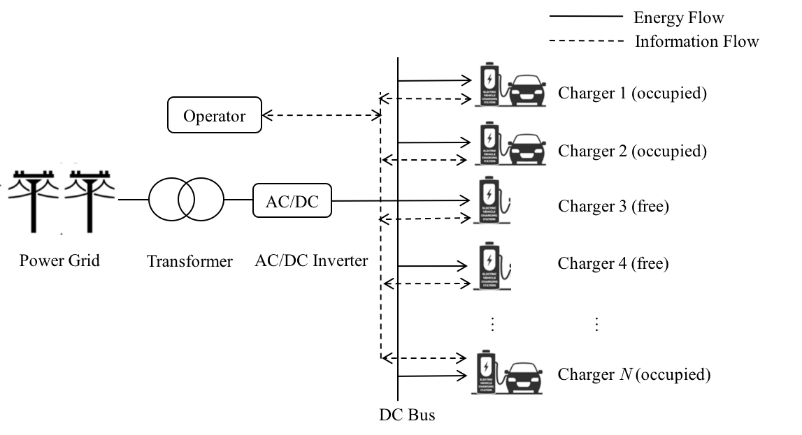
Figure 2: Schematic of EV charging scheduling

Some of the key details of the EV charging problem and assumptions are outlined below.

A1)

All the chargers with a constant charging rate $R$ are available at any stage $t\in\mathcal{T}$. The charging decision at stage $t$ for the $i$th charger is a binary variable $u_{i,t}\in\{0,1\}$, with $1$ activating and $0$ deactivating the charging port. We also denote $M$ as the maximum number of simultaneous chargers allowed by the maximum power constraint of the local transformer, where $M<N$.

A2)

The peak average consumption used to compute the demand charge is represented by variable $\psi$. In the case of EV charging, we assume the demand charge is a linear function $\mathcal{C}(\psi)=\pi^{d}\psi$ with the demand charge price $\pi^{d}$.

A3)

The EV arriving at the $i$th charger at the beginning of stage $t_{0}$ reveals random $D_{i,t_{0}}$ (the total amount of energy to be completed) and $T_{i,t_{0}}$ (the time for completion). An EV will be automatically removed at the end of its completion time. An EV arriving at charger $i$ will be rejected if charger $i$ has been already occupied.

A4)

The operator receives a per unit reward $\pi^{r}$ and pays a time-varying charging cost $\pi^{e}_{t}$ if it serves an EV at stage $t$. For simplicity, we assume that parameters $\pi^{r}$ and $\{\pi^{e}_{t}\}_{t=0}^{T-1}$ are deterministic. The proposed approaches can be easily extended towards stochastic settings.

A5)

If the total charging demand of EV $i$ is not completed at its completion time, then a penalty $qz_{i}$ occurs at price $q$, and $z_{i}$ denotes the amount of unmet demand. For simplicity, we assume that the penalty price is greater than the largest charging cost over the whole horizon, i.e., $q\geq\pi^{e}_{t},~{}\forall t\in\mathcal{T}$.

IV-B EV Charging as DLS-DC

We now define the DLS-DC model described in Section II for the EV charging problem.

IV-B1 Exogenous Stochastic Input $\bm{\xi}=(\xi_{i,t})$

The input of DLS-DC model is a vector random process that models the arrivals of deferrable demands at individual chargers. The occupancy of each charger is an on-off process with the charger being occupied for the duration of the EV charging deadline and being idle for the duration of a Bernoulli process with parameter $p_{i}$ set by the overall arrival rate of the EV demand. At the beginning of an occupied period of charger $i$, say at $t_{0}$, an EV arrives with random energy demand $D_{i,t_{0}}$ and random deadline $T_{i,t_{0}}$. Thus the input process at charger $i$ is given by $\xi_{i,t}=(D_{i,t_{0}},T_{i,t_{0}})$ for $t=t_{0},\cdots,T_{i,t_{0}}$. When the charger is idle, $\xi_{i,t}=(0,0)$. With probability $p_{i}$, $\xi_{i,t}=(0,0)$ transitions to $\xi_{i,t+1}=(D_{i,t+1},T_{i,t+1})$.

IV-B2 System State and State Evolution

The state of charger $i$ at stage $t$ is given by a tuple $x_{i,t}=(r_{i,t},\tau_{i,t})$, where $r_{i,t}$ represents the remaining demand to be served by deadline $T_{i,t}$ at charger $i$ and $\tau_{i,t}=T_{i,t}-t$ the lead time to the EV’s completion at stage $t$. Hence, the system state is modeled as

$$x_{i,t+1}=\begin{cases}x_{i,t}-(u_{i,t},1)&~{}\text{if}~{}\tau_{i,t}>1,\\ \xi_{i,t}&~{}\text{if}~{}\tau_{i,t}\leq 1.\end{cases}$$ (18)

Note that when the charger is free, its state is $(0,0)$. When there is no EV arriving at charger $i$, the state of the charger remains at $(0,0)$.

IV-B3 Constraints

The total amount of power used for charging at one stage is limited by

$$\sum_{i=1}^{N}{u_{i,t}}\leq M,~{}t\in\mathcal{T}.$$ (19)

As shown in A2), the peak average demand $\psi$ over $\ell$ intervals is

$$\psi=\max_{t\in\mathcal{T}^{\prime}}~{}{\frac{R}{\ell}\sum_{\tau=t}^{t+\ell-1}{\sum_{i=1}^{N}{u_{i,\tau}}}}.$$ (20)

IV-B4 Stage Reward

The stage reward collected from all the EVs at stage $t$ is given by

$$\mathcal{G}_{t}(\mathbf{x}_{t},\mathbf{u}_{t},\bm{\xi}_{t})=R\Delta\left[(\pi^{r}-\pi_{t}^{e})\sum_{i=1}^{N}{u_{i,t}}-q\sum_{i\in\mathcal{J}_{t}}{(r_{i,t}-u_{i,t})}\right]$$ (21)

where $\Delta$ denotes the length of a scheduling stage and $\mathcal{J}_{t}$ the set of EVs that will leave at stage $t+1$, i.e., $\mathcal{J}_{t}:=\{i:\tau_{i,t}=1\}$.

IV-B5 MDP formulation

The objective of EV scheduling is to find the optimal control policy $\{\mu_{t}^{*}\}_{t\in\mathcal{T}}$ to maximize the expected total reward in the presence of the demand charge. At each stage $t$, a control law maps states to controls:

$$\mathbf{u}_{t}=\mu_{t}(\mathbf{x}_{t},\bm{\xi}_{t}).$$ (22)

Given an initial state $\mathbf{x}_{0}$, the EV schedule system can be formulated as

$$\max_{\{\mu_{t}\}_{t\in\mathcal{T}}}{} {\mathbb{E}\left[\sum_{t=0}^{T-1}{\mathcal{G}_{t}(\tilde{\mathbf{x}}_{t},\tilde{\mathbf{u}}_{t},\bm{\xi}_{t})}-\pi^{d}\psi\right]}$$ (23)

s.t. $$\eqref{eqn:EV_state}\eqref{eqn:EV_power}\eqref{eqn:EV_dc}\eqref{eqn:policy_to_state},$$

$$\text{initializing}~{}\tilde{\mathbf{x}}_{0}=\mathbf{x}_{0}.$$

With (23), various MPC solutions, including the proposed BMPC approach, can be implemented.

V Numerical Results

We conducted simulations involving stochastic EV-charging demands with random arrival times, charging demands and deadlines for completion. We assumed that the number of newly arrived EVs at each stage followed a Poisson distribution. The charging demand and completion time of a new EV followed uniform distributions $\mathcal{U}(0,D_{\text{max}})$ and $\mathcal{U}(0,T_{\text{max}})$ respectively.

All prices were deterministic. The electricity prices were from the Electric Reliability Council of Texas (ERCOT). The penalty price $q$ was set as 0.3 $/kWh. In numerical simulations, we varied the demand charge price $\pi^{d}$ from 6 $/kW to 21 $/kW [24], where the length of the measurement window was fixed at 15 minutes and billing period a whole month. Other parameters are summarized in Table I.

TABLE I: Parameter settings

Parameter	Value	Note
$N$	50	Total Number of Chargers
$R$	240 kW	Constant Charging Power
$M$	25	Maximum Number of Simultaneous Chargers
$\lambda$	5	Expected EV Arrival Rate
$D_{\text{max}}$	120 kWh	Maximum Energy Demand
$T_{\text{max}}^{d}$	1 hour	Maximum Completion Time

V-A Benchmark and Performance

To compare with BMPC, we adopted both MPC-based approaches (NMPC and EMPC, see Section III-C) and index rules (EDF [16] and LLF-LD [15]) as the benchmark methods. For each sampled trajectory, we ran each algorithm and computed its total reward gap to the upper bound (in percentage) as the performance measure. Suppose we obtained $S$ sampled trajectories for all EV charging requests across time $\{\bm{\xi}_{t}^{s},t=0,\dots,T\}_{s=1}^{S}$. We then solved an integer program that defined the deterministic DLS-DC for the upper bound of the total reward on the $s$th trajectory:

$$\max_{\{\tilde{\mathbf{u}}_{t}\}_{t\in\mathcal{T}}}{} \sum_{t=0}^{T-1}{\mathcal{G}_{t}(\tilde{\mathbf{x}}_{t},\tilde{\mathbf{u}}_{t},\bm{\xi}_{t}^{s})}-\pi^{d}\psi$$ (24)

s.t. $$\eqref{eqn:EV_state}\eqref{eqn:EV_power}\eqref{eqn:EV_dc},$$

$$\text{initializing}~{}\tilde{\mathbf{x}}_{0}=\mathbf{x}_{0}.$$

By solving (24), we also obtained the optimum of the maximum average consumption measured by the demand charge for each trajectory. For a given demand charge price, we simulated all methods over $S=100$ scenarios with randomly generated EV charging requests, and reported the average performances over these scenarios.

V-B Multi-resolution DLS-DC

In practice, the resolution of control can be significantly finer than that of the demand-charge measurement. For example, the measurement window size can be 15 minutes whereas the EV charging decisions can be made at the one to five minute resolution, i.e. $\ell=3\sim 15$. The results presented in this section are from simulations with $\ell=3$, i.e., $\Delta=5$ minutes.

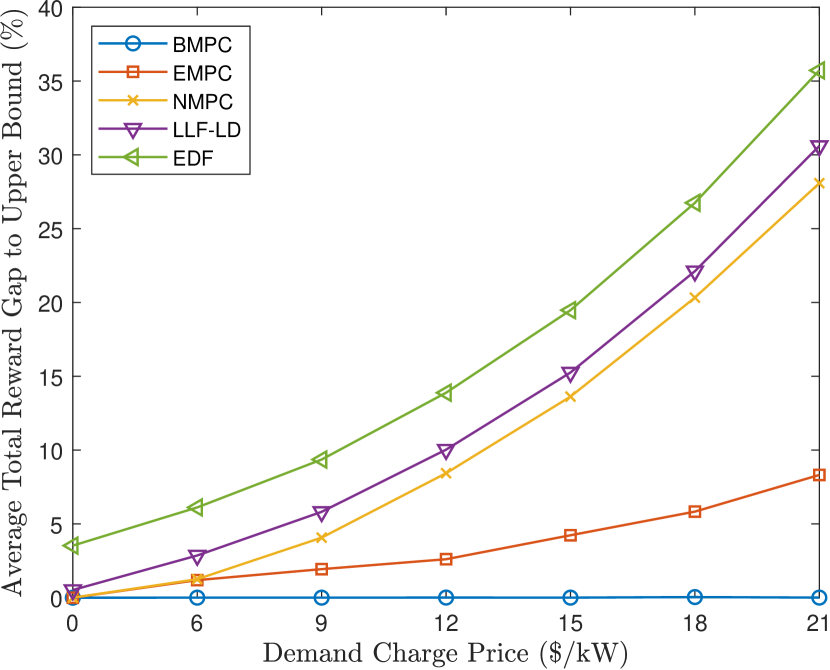
(a) perfect forecast

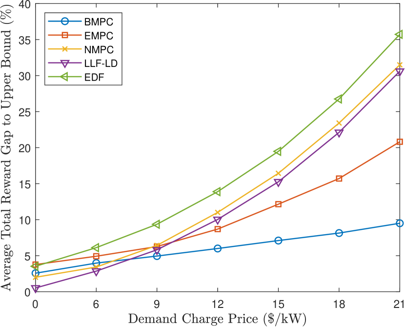
(b) imperfect forecast

Figure 3: Average performance gap to upper bound with multi-resolution scheduling ($\ell=3$).

V-B1 Perfect Forecast

In this case, we assumed that accurate information on EV arrivals, charging demands and required completion times were available, e.g., via reservation apps.

Fig. 3(a) compared the performance of BMPC with other methods under different demand charge prices (x-axis). The y-axis of Fig. 3(a) showed the average optimality gaps between each method and the upper bound over all the sampled trajectories. We observed that BMPC outperformed other methods that did not consider the demand charge. In particular, BMPC almost reached upper bound ($0.16\%$ gaps), and achieved 27% higher reward on average than NMPC. EMPC, however, performed worse than BMPC when $\ell=3$. As mentioned in Section III-C, this was due to the mismatch between the actual peak values of the reference trajectory and those requested by EMPC. As shown in Table II, we observed that although both BMPC and EMPC managed to reduce the peak consumption as the demand charge price went higher, the peak consumption of EMPC deviated from the optimal one, which degraded its performance by at most 8% compared to BMPC.

TABLE II: Maximum average power consumption (MW) with multi-resolution scheduling ($\ell=3$) under forecast (Others: NMPC, LLF-LD and EDF)

DC price ($/MW)		0	6	9	12	15	18	21
Optimal		6.00	4.96	4.88	4.56	4.56	4.32	4.24
perfect   forecast	BMPC	6.00	4.96	4.88	4.56	4.56	4.32	4.24
	EMPC	6.00	5.28	5.04	5.04	5.04	4.80	4.80
	Others	6.00	6.00	6.00	6.00	6.00	6.00	6.00
imperfect   forecast	BMPC	6.00	4.96	4.88	4.56	4.56	4.32	4.24
	EMPC	5.04	5.04	5.04	5.04	5.04	5.04	5.04
	Others	6.00	6.00	6.00	6.00	6.00	6.00	6.00

V-B2 Imperfect Forecast

We considered a slightly more complicated setting, where the EV arrivals, charging demands and required completion times were random. For BMPC and NMPC, the forecasts on exogenous process $\bm{\xi}$ were based on the mean trajectories. The computation of forecasted reference trajectory of EMPC was demonstrated in Appendix A.

It was worth noting that BMPC may need to modify the schedule at certain stages, since it took a block of controls based on the inaccurate information for the near future. For example, BMPC would commit to the charging actions $\{\mathbf{\tilde{u}}^{*}_{t},\mathbf{\tilde{u}}^{*}_{t+1},\cdots,\mathbf{\tilde{u}}^{*}_{t+\ell-1}\}$ after solving (5) at stage $t$. The subsequent actions from $\mathbf{\tilde{u}}^{*}_{t}$, which were optimal for the predicted EV trajectory, might become infeasible for the realized EV profile. One simple solution to this issue was to deactivate the chargers that were conducting the infeasible actions whenever such rescheduling was necessary.

Similar with Fig. 3(a), Fig. 3(b) quantified the average gaps between all methods and the upper bound. Due to the potentially suboptimal rescheduling actions of BMPC, LLF-LD achieved the best performance when the demand charge was small (e.g., $\pi^{d}\leq 6$ $/kW in Fig. 3(b)). In such a regime, the reward from scheduling played a more important role than the demand charge cost, and the peak differences among all the methods were relatively small (see Table II), which made the MPC-based methods less average total reward due to prediction errors. When the demand charge price was relatively high, the savings on the demand charge that BMPC achieved dominated the penalties due to the rescheduling, thus BMPC outperformed other methods and achieved nearly 20% more average total reward than LLF-LD at 21 $/kW. Meanwhile, the performance of EMPC further downgraded to at most 10% gap to BMPC and 20% to the upper bound, since both of mismatching in peak information and following an inaccurate reference trajectory came into effect.

V-C Single-resolution DLS-DC

This section validates the case when the resolution of peak-consumption measurement matched that of the decision, i.e. $\ell=1$ ($\Delta=15$ minutes). In this case, BMPC operated at the same timescales as NMPC and EMPC.

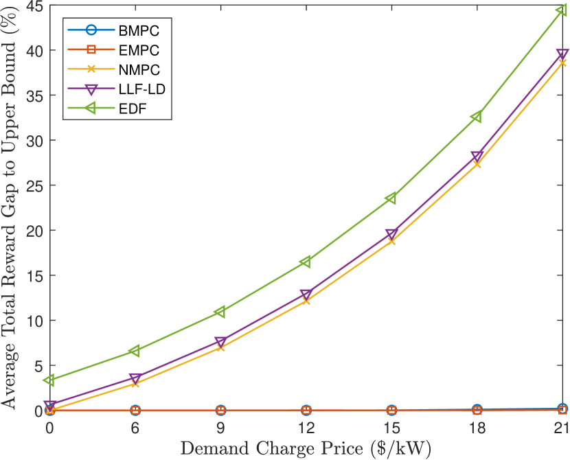
(a) perfect forecast

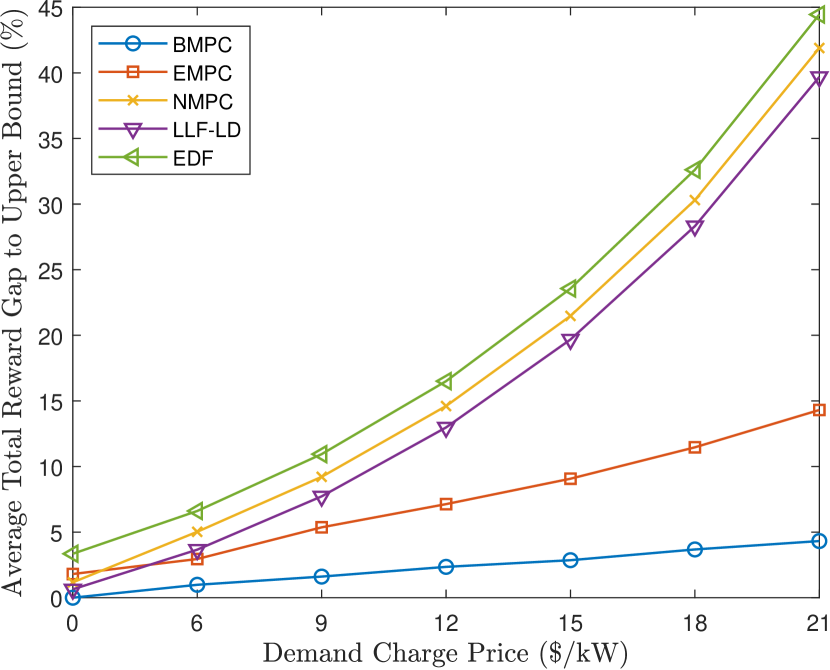
(b) imperfect forecast

Figure 4: Average performance gap to upper bound with single-resolution scheduling ($\ell=1$).

TABLE III: Maximum average consumption (MW) with single-resolution scheduling ($\ell=1$) under forecast (Others: NMPC, LLF-LD and EDF)

DC price ($/MW)		0	6	9	12	15	18	21
Optimal		6.00	4.32	4.08	4.08	3.84	3.60	3.36
perfect   forecast	BMPC	6.00	4.32	4.08	4.08	3.84	3.60	3.36
	EMPC	6.00	4.32	4.08	4.08	3.84	3.60	3.36
	Others	6.00	6.00	6.00	6.00	6.00	6.00	6.00
imperfect   forecast	BMPC	6.00	4.32	4.08	4.08	3.84	3.60	3.36
	EMPC	5.04	4.32	4.32	4.32	4.32	4.32	4.32
	Others	6.00	6.00	6.00	6.00	6.00	6.00	6.00

V-C1 Perfect Forecast

We first considered the case with accurate information on EVs. As shown in Fig. 4(a), the best method was EMPC, which reached upper bound (almost $0\%$ gaps at all the demand charge prices) because it tracked the optimal reference trajectory. BMPC achieved similar performances but with slightly bigger gaps ($0.17\%$). The other methods (NMPC, LLF-LD and EDF), which did not take the demand charge into account, all experienced rapid growth of the optimality gaps due to the large demand charge costs.

Table III further compared all methods in terms of peak consumption over the whole month. Both BMPC and EMPC reduced peak charging power as the demand charge prices increased, whereas the other methods failed to reduce the peak consumption thus reached the total charging limit 6 MW at all the demand charge prices.

V-C2 Imperfect Forecast

We then considered imperfect forecasts on EVs. Predictions were generated using the same method as shown in Section V-B.

Due to prediction errors, all MPC-based methods had positive gaps. We observed that BMPC was the best method with optimality gaps less than 5%. EMPC, however, was no longer the best choice. EMPC achieved 10% less reward than BMPC when the demand charge price was at 21 $/kW. The main reason for the marked gap increase was that it tracked an untrustworthy reference trajectory. Since LLF-LD and EDF did not require predictions, their performances remained the same as the perfect forecast case.

V-D Discussions

Figs. 3 and 4 also illustrated the performance of NMPC, EDF, and LLF-LD. Comparing with BMPC and EMPC, the suboptimal performances of these methods were consequences of not considering the demand charge costs.

As shown in all figures, EDF was always the one with the least total reward in all cases. EDF was a simplistic and myopic scheduling policy; it failed to meet many charging requests thus suffered from large penalties.

In the cases with perfect forecast (see Figs. 3(a) and 4(a)), NMPC performed slightly better than LLF-LD. In the cases with imperfect forecast (see Figs. 3(b) and 4(b)), LLF-LD surpassed NMPC. This was because predictions were not required to run LLF-LD. It should be noted that, as an index-like policy, LLF-LD had much lower computation cost than MPC-based techniques, and it performed the best when the demand charge was relatively low.

VI Conclusion

We consider the problem of DLS-DC, which can be widely adopted to applications such as scheduling of EV charging and cloud computing services. Due to the difficulties of multiple timescales posed by the demand charge pricing, we propose the BMPC algorithm with a special terminal cost to incorporate the demand charge at each scheduling stage. Through a motivating application of EV charging scheduling, our proposed approach shows advantageous performances compared to the benchmark methods, highlighting the significant impact of demand charge for deferrable load scheduling.

Appendix A Selected Benchmark Solutions

A-1 Reference Trajectory of Economic MPC [25]

Here we introduce the computation of a reference trajectory for EMPC under stochastic settings. We assume the random inputs $\{\xi_{t}\}_{t=0}^{T-1}$ follow an arbitrary distribution with expectation at $\overline{\xi}$, then a forecasted reference trajectory can be computed by solving the following deterministic DLS-DC:

$$\max_{\{\tilde{u}_{t}\}_{t\in\mathcal{T}}}~{} \sum_{t\in\mathcal{T}}{\mathcal{G}_{t}(\tilde{x}_{t},\tilde{u}_{t},\overline{\xi})}-\mathcal{C}(\psi)$$ (25a)

s.t. $$\tilde{x}_{t+1}=f_{t}(\tilde{x}_{t},\tilde{u}_{t},\overline{\xi}),\quad t\in\mathcal{T}$$ (25b)

$$h_{t}(\tilde{x}_{t},\tilde{u}_{t},\overline{\xi})\leq 0,\quad t\in\mathcal{T}$$ (25c)

$$u_{t}=\mu_{t}(\tilde{x}_{t},\overline{\xi}),\quad t\in\mathcal{T}$$ (25d)

$$\tilde{x}_{0}=x_{0},$$ (25e)

$$\psi=\max_{t\in\mathcal{T^{\prime}}}~{}\left\{\frac{1}{\ell}\sum_{\tau=t}^{t+\ell-1}{c(\tilde{x}_{\tau},\tilde{u}_{\tau},\overline{\xi})}\right\}.$$ (25f)

By denoting $(\mathbf{x}^{\text{ref}},\mathbf{u}^{\text{ref}})$ as the optimal solution of (25), the forecasted reference trajectory can be obtained as $(\mathbf{x}^{\text{ref}},\mathbf{u}^{\text{ref}},\overline{\bm{\xi}})$.

A-2 Earliest Deadline First (EDF)[16]

EDF is a rather simple online scheduling rule for deferrable loads. Specifically, at each stage $t$, it gives priorities to tasks with the earliest deadlines and tries to serve as many tasks as possible. Therefore, EDF would use the full power limit when the demand is heavy, resulting in large cost on demand charge.

A-3 Least Laxity First with Later Deadline (LLF-LD) [15]

LLF-LD is an online algorithm for deferrable load scheduling, which prioritizes tasks with less laxity at each stage. Laxity, as defined in [15], is the difference between a server’s lead time and its remaining processing time, reflecting the maximum number of stages that a task can tolerate before the time it has to be continuously processed to avoid non-completion penalty. For the EV charging problem in Section IV, the laxity of an EV at charger $i$ at stage $t$ is $\tau_{i,t}-r_{i,t}$. If the laxity of two tasks are the same, then it prioritizes the one with later deadline. Note that LLF-LD would also fully utilize the grid capacity as EDF, which results in significant amount of demand charge.

References

- [1] T.-H. Chang, M. Alizadeh, and A. Scaglione, “Real-time power balancing via decentralized coordinated home energy scheduling,” IEEE Transactions on Smart Grid, vol. 4, no. 3, pp. 1490–1504, 2013.
- [2] H. Hao, B. M. Sanandaji, K. Poolla, and T. L. Vincent, “Aggregate flexibility of thermostatically controlled loads,” IEEE Transactions on Power Systems, vol. 30, no. 1, pp. 189–198, 2014.
- [3] N. Chen, L. Gan, S. H. Low, and A. Wierman, “Distributional analysis for model predictive deferrable load control,” in 53rd IEEE Conference on Decision and Control. IEEE, 2014, pp. 6433–6438.
- [4] M. Rahmani-Andebili, “Scheduling deferrable appliances and energy resources of a smart home applying multi-time scale stochastic model predictive control,” Sustainable Cities and Society, vol. 32, pp. 338–347, 2017.
- [5] S. Chen and L. Tong, “iEMS for large scale charging of electric vehicles: Architecture and optimal online scheduling,” in 2012 IEEE Third International Conference on Smart Grid Communications (SmartGridComm), 2012, pp. 629–634.
- [6] Y. Xu and F. Pan, “Scheduling for charging plug-in hybrid electric vehicles,” in 2012 IEEE 51st IEEE Conference on Decision and Control (CDC). IEEE, 2012, pp. 2495–2501.
- [7] D. T. Nguyen and L. B. Le, “Joint optimization of electric vehicle and home energy scheduling considering user comfort preference,” IEEE Transactions on Smart Grid, vol. 5, no. 1, pp. 188–199, 2013.
- [8] Q. Huang, Q.-S. Jia, Z. Qiu, X. Guan, and G. Deconinck, “Matching EV charging load with uncertain wind: A simulation-based policy improvement approach,” IEEE Transactions on Smart Grid, vol. 6, no. 3, pp. 1425–1433, 2015.
- [9] Z. Yu, S. Chen, and L. Tong, “An intelligent energy management system for large-scale charging of electric vehicles,” CSEE Journal of Power and Energy Systems, vol. 2, no. 1, pp. 47–53, 2016.
- [10] Y. Xu, F. Pan, and L. Tong, “Dynamic scheduling for charging electric vehicles: A priority rule,” IEEE Transactions on Automatic Control, vol. 61, no. 12, pp. 4094–4099, 2016.
- [11] G. Zhang, S. T. Tan, and G. G. Wang, “Real-time smart charging of electric vehicles for demand charge reduction at non-residential sites,” IEEE Transactions on Smart Grid, vol. 9, no. 5, pp. 4027–4037, 2017.
- [12] C. Le Floch, S. Bansal, C. J. Tomlin, S. J. Moura, and M. N. Zeilinger, “Plug-and-play model predictive control for load shaping and voltage control in smart grids,” IEEE Transactions on Smart Grid, vol. 10, no. 3, pp. 2334–2344, 2017.
- [13] M. Dabbagh, B. Hamdaoui, A. Rayes, and M. Guizani, “Shaving data center power demand peaks through energy storage and workload shifting control,” IEEE Transactions on Cloud Computing, 2017.
- [14] Z. Yu, Y. Xu, and L. Tong, “Deadline scheduling as restless bandits,” IEEE Transactions on Automatic Control, vol. 63, no. 8, pp. 2343–2358, 2018.
- [15] J. Jin and Y. Xu, “Priority rules on the charging of electric vehicles with energy storage,” 2019.
- [16] C. L. Liu and J. W. Layland, “Scheduling algorithms for multiprogramming in a hard-real-time environment,” Journal of the ACM (JACM), vol. 20, no. 1, pp. 46–61, 1973.
- [17] A. K.-L. Mok, “Fundamental design problems of distributed systems for the hard-real-time environment,” Ph.D. dissertation, Massachusetts Institute of Technology, 1983.
- [18] A. Di Giorgio, F. Liberati, and S. Canale, “Electric vehicles charging control in a smart grid: A model predictive control approach,” Control Engineering Practice, vol. 22, pp. 147–162, 2014.
- [19] J. L. Neufeld, “Price discrimination and the adoption of the electricity demand charge,” Journal of Economic History, pp. 693–709, 1987.
- [20] Z. Wang, B. Asghari, and R. Sharma, “Stochastic demand charge management for commercial and industrial buildings,” in 2017 IEEE Power & Energy Society General Meeting. IEEE, 2017, pp. 1–5.
- [21] Y. Zhang and G. Augenbroe, “Optimal demand charge reduction for commercial buildings through a combination of efficiency and flexibility measures,” Applied Energy, vol. 221, pp. 180–194, 2018.
- [22] H. Xu and B. Li, “Reducing electricity demand charge for data centers with partial execution,” in Proceedings of the 5th international conference on Future energy systems, 2014, pp. 51–61.
- [23] R. Kumar, M. J. Wenzel, M. J. Ellis, M. N. ElBsat, K. H. Drees, and V. M. Zavala, “A stochastic model predictive control framework for stationary battery systems,” IEEE Transactions on Power Systems, vol. 33, no. 4, pp. 4397–4406, 2018.
- [24] J. Jin and Y. Xu, “Optimal storage operation under demand charge,” IEEE Transactions on Power Systems, vol. 32, no. 1, pp. 795–808, 2016.
- [25] M. J. Risbeck and J. B. Rawlings, “Economic model predictive control for time-varying cost and peak demand charge optimization,” IEEE Transactions on Automatic Control, vol. 65, no. 7, pp. 2957–2968, 2020.