Abstract

We perform a comprehensive and model-independent analysis for characterizing the spin and dynamical structure of the production of a non-diagonal pair of Majorana particles with different masses and arbitrary spins, $e^{-}e^{+}\to X_{2}X_{1}$, followed by a sequential two-body decay, $X_{2}\to ZX_{1}$, of the heavier particle $X_{2}$ into a $Z$ gauge boson and the lighter particle $X_{1}$ escaping undetected at high-energy $e^{+}e^{-}$ colliders. Standard leptonic $Z$-boson decays, $Z\to\ell^{-}\ell^{+}$ with $\ell=e$ or $\mu$, are employed for precisely diagnosing the $Z$ polarization influenced by the production and decay processes. Based on helicity formalism and Wick helicity rotation for describing the correlated production-decay amplitudes and distributions, we work out the implications on the amplitudes and distributions of discrete CP symmetry and the Majorana condition that two particles are their own anti-particles. For the sake of a concrete illustration, an example of this type in the minimal supersymmetric Standard Model is investigated in detail.

1 Introduction

The Standard Model (SM) [1, 2, 3] has been firmly confirmed as a self-consistent gauge theory with a weakly-coupled sector for electroweak (EW) symmetry breaking with the discovery of a scalar boson [4, 5] and the ever-increasing confidence of its compatibility with the SM Higgs boson [6, 7] at the CERN Large Hadron Collider (LHC). Nevertheless, we highly expect new physics beyond the SM (BSM) to be revealed at the TeV scale (Terascale), motivated by tiny but non-vanishing neutrino masses [8], matter dominance in our Universe [9, 10], dark matter [11, 12, 13] and inflation [14], etc. Conceptually, the naturalness issue [15, 16, 17] has been the prime argument for the realization of new BSM physics at the weak scale of 246 GeV.

To much puzzlement, except for a SM-like Higgs boson, no new BSM particles have been so far observed in the LHC experiments around the Terascale threshold. One plausible scenario for the LHC null search results is that all the strongly-interacting colored BSM particles are too heavy to be directly produced at the LHC and the electroweak (EW) BSM particles, although kinematically accessible, may not lead to tractable signals due to rather small production rate, uncharacteristic signature and/or large SM backgrounds at hadron colliders. On the other hand, the future high-energy $e^{+}e^{-}$ colliders would be capable of discovering and diagnosing some new EW particles, as long as kinematically accessible, because of well-constrained event topology and very clean experimental environment.

In the present work, we study such a challenging but plausible scenario at an $e^{+}e^{-}$ collider that two neutral BSM particles are kinematically accessible only with the combination of the diagonal pair of the lighter particles and the non-diagonal pair of two particles, while the diagonal pair of the heavier particles is kinematically inaccessible, see for example Ref. [18]. Particularly, two neutral particles are assumed to be their own antiparticles but their spins are arbitrary. Such Majorana particles  are unavoidable in supersymmetric theories, guaranteeing that every known bosonic particle has a heavier fermionic partner and vice versa for each known fermion, and they are predicted also by various grand unified theories and extra-dimensional models and even in solid-state physics [19].

Referring to Refs. [20, 21] as a few previous works for the processes of diagonal pair production, we focus on the analysis of the combined process of production of a non-diagonal pair of Majorana particles with different masses and arbitrary spins, followed by a sequential decay chain of two-body decays as

$$e^{-}\,+\,e^{+}\, \to \,X_{2}\,+\,X_{1}$$ (1)

$$\ \ \rotatebox[origin={c}]{180.0}{\Large$\Lsh$}\ \ Z\,+\,X_{1}$$

$$\ \ \qquad\rotatebox[origin={c}]{180.0}{\Large$\Lsh$}\ \ \ell^{-}\,+\,\ell^{+}\,,$$

where the mass splitting $\Delta m=m_{2}-m_{1}$ of the particles $X_{2}$ and $X_{1}$ is larger than the $Z$ boson mass $m_{Z}$, i.e. $m_{2}-m_{1}>m_{Z}$, and the charged lepton $\ell$ is taken to be $e$ or $\mu$, allowing for the full reconstruction of the $Z$-boson momentum with great precision.

The neutral particle $X_{1}$ is assumed to be stable and so it escapes undetected with no tractable signals as the lightest neutral supersymmetric particle (LSP) in the minimal supersymmetric SM (MSSM) with $R$ parity. Consequently, the combined process has a distinct $V$-shape signature of a charged-lepton pair of which the four-momentum is balanced due to energy-momentum conservation with the missing four-momentum carried away by two invisible $X_{1}$ particles

$$e^{-}e^{+}\ \ \rightarrow\ \ \ell^{-}\ell^{+}\,+\,\not\!\!{E}\,,$$ (2)

with $\not\!\!{E}$ denoting the invisible part and with the constraint $m_{\ell\ell}=m_{Z}$ for the invariant mass of two final leptons, signalling the presence of an intermediate on-shell $Z$ boson.

For a non-zero $X_{2}$ spin $j_{2}$, the $X_{2}$ particle is produced generally in a polarized state in the process (1), especially, if the interactions are parity-violating. The information on the polarization of the spin-1 gauge boson $Z$ can be extracted through the angular distributions in its well-established leptonic decays, $Z\to\ell^{-}\ell^{+}$, with $\ell=e$ or $\mu$. However, the $Z$ momentum direction in the $X_{2}$ rest frame ($X_{2}$RF) which is the most convenient for describing the decays analytically is not identical to that in the $e^{+}e^{-}$ CM frame ($ee$CM) directly reconstructed experimentally. A proper Wick helicity rotation [22, 23, 24] needs to be incorporated for linking the $Z$ polarization state with respect to the $Z$ momentum direction in the $ee$CM to that with respect to the $Z$ momentum direction in the $X_{2}$RF.

The prime goal of the present work is to derive the correlated production-decay (polar-)angular correlations in a transparent and compact way exploiting the helicity formalism and an Wick helicity rotation for probing the spins and dynamical properties of two Majorana particles in a general setting.

The paper is organized as follows. In Section 2, we present the complete amplitudes of the production process and two sequential two-body decays in a compact and general form and analyze the implications of the discrete CP symmetry and the Majorana condition on the amplitudes and production-decay correlations. Section 3 is devoted to a systematic derivation of all the angular correlations and a detailed analysis of the fully-reconstructible polar-angle correlations. In Section 4 those model-independent theoretical results are demonstrated with one specific example of a non-diagonal pair of neutralinos [25, 26, 27, 28, 29, 30], which are Majorana fermions in the MSSM. Finally some conclusions are given in Section 5.

2 Production and Decay Amplitudes

In this section, firstly we present in a compact and transparent form the complete helicity amplitudes for the production of a nondiagonal pair of Majorana particles and for the two sequential two-body decays shown in Eq. (1), of which the kinematical configuration is depicted in detail in Figure 1. A proper Wick helicity rotation and an azimuthal-angle adjustment are performed for linking the decay helicity amplitudes in the $X_{2}$RF and $ee$CM. Secondly, we remark on the general constraints on the amplitudes by CP invariance and by the Majorana condition.

2.1 Helicity amplitudes

We adopt the helicity formalism [22, 31] for deriving the helicity amplitudes of the production process for a nondiagonal pair $X_{2}X_{1}$ of Majorana particles

$$e^{-}(k,\sigma)\,+\,e^{+}(\bar{k},\bar{\sigma})\ \ \rightarrow\ \ X_{2}(p_{2},\lambda_{2})\,+\,X_{1}(p_{1},\lambda_{1})\,,$$ (3)

in the $e^{-}e^{+}$ center-of-mass (CM) frame ($ee$CM), and those of the two-body decay of the Majorana particle $X_{2}$ of mass $m_{2}$ and spin $j_{2}$ into an on-shell spin-1 $Z$ boson of mass $m_{Z}$ and a Majorana particle $X_{1}$ of mass $m_{1}$ and spin $j_{1}$

$$X_{2}(p^{\prime}_{2},\lambda_{2})\ \ \rightarrow\ \ Z(q_{Z},\lambda_{Z})\,+\,X_{1}(q_{1},\sigma_{1})\,,$$ (4)

in the $X_{2}$RF (See Refs. [23, 34] for the neutralino two-body decay in the MSSM) and for the $Z$ two-body leptonic decay

$$Z(q^{\prime}_{Z},\lambda^{\prime}_{Z})\ \ \rightarrow\ \ \ell^{-}(k_{-},\tau_{-})\,+\ell^{+}(k_{+},\tau_{+})\,,$$ (5)

in the $Z$ rest frame ($Z$RF). The four-momentum and helicity of each particle are shown in parenthesis with each primed four-momentum referring to the four-momentum in the rest frame of its corresponding particle, $X_{2}$ or $Z$. One crucial point to be ensured in calculating the amplitudes of the correlated production-decay process is that the $Z$-boson polarization state in the $X_{2}$RF is in general different from that in the $Z$RF directly reconstructible in the $ee$CM.

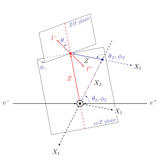
Figure 1: A diagrammatic description of kinematical configurations of the combined production-decay process (1). The $X_{2}$ polar and azimuthal angles, $\theta_{2}$ and $\phi_{2}$, are defined with respect to the $e^{-}$ momentum direction and a properly chosen $x$-axis. The $Z$ polar and azimuthal angles, $\theta_{Z}$ and $\phi_{Z}$, are defined in the $X_{2}$ rest frame boosted back along the $X_{2}$ momentum direction from the $ee$CM and the $\ell^{-}$ polar and azimuthal angles, $\theta_{-}$ and $\phi_{-}$, are defined in the $Z$ rest frame boosted back along the $Z$ momentum direction in the $ee$CM, respectively. The azimuthal angle $\phi_{-}$ denotes the relative angle between the $eeZ$ plane and the $Z\ell\ell$ plane in the $ee$CM.

Explicitly, in the kinematical configuration depicted in Figure 1, the helicity amplitude of the production process $e^{-}e^{+}\to X_{2}X_{1}$ can be written as

$${\cal M}^{e^{-}e^{+}\to X_{2}X_{1}}_{\sigma,\bar{\sigma};\lambda_{2},\lambda_{1}}(\theta_{2},\phi_{2})={\cal P}_{\sigma,\bar{\sigma};\lambda_{2},\lambda_{1}}(\cos\theta_{2})\,\,d^{J}_{\sigma-\bar{\sigma},\lambda_{2}-\lambda_{1}}(\theta_{2})\,e^{\imath(\sigma-\bar{\sigma})\phi_{2}}\,,$$ (6)

where $J={\rm max}(|\sigma-\bar{\sigma}|,|\lambda_{2}-\lambda_{1}|)$, and the angles $\theta_{2}$ and $\phi_{2}$ denote the scattering polar and azimuthal angles of the $X_{2}$ with respect to the $e^{-}$ momentum direction and a fixed $x$-axis, of which the direction may be fixed for transverse $e^{-}$ or $e^{+}$ beam polarizations, in the $ee$CM. Finally the polar-angle dependent function $d^{J}_{\sigma-\bar{\sigma},\lambda_{2}-\lambda_{1}}(\theta_{2})$ is the Wigner $d$ function in the convention of Rose [32].

The general theoretical analysis of the $Z$ polarization in the two-body decay $X_{2}\to ZX_{1}$ is the most transparent analytically in the $X_{2}$RF. The decay helicity amplitude can be decomposed in terms of the decay polar and azimuthal angles, $\theta_{Z}$ and $\phi_{Z}$, for the momentum direction of the $Z$ boson in the $X_{2}$RF

$${\cal M}^{X_{2}\to ZX_{1}}_{\lambda_{2};\lambda_{Z},\sigma_{1}}(\theta_{Z},\phi_{Z})={\cal C}_{\lambda_{Z},\sigma_{1}}\,d^{j_{2}}_{\lambda_{2},\lambda_{Z}-\sigma_{1}}(\theta_{Z})\,e^{i\lambda_{2}\phi_{Z}}\quad\mbox{with}\quad|\lambda_{Z}-\sigma_{1}|\leq j_{2}\,,$$ (7)

where the azimuthal angle $\phi_{Z}$ is defined with respect to the plane formed by the $e^{-}$ and $X_{2}$ momenta in the $ee$CM. Because the $Z$-momentum direction in the $X_{2}$RF is different from that in the $ee$CM, the helicity amplitudes in Eq. (7) need to be transformed by a proper Wick helicity rotation [22, 23, 24] for connecting the $Z$ helicity state in the $X_{2}$RF to that in the $ee$CM with a so-called Wick helicity rotation angle $\omega_{{}_{Z}}$ satisfying

$$\cos\omega_{{}_{Z}} = \frac{\beta_{Z}+\beta_{2}\cos\theta_{Z}}{\sqrt{(1+\beta_{2}\beta_{Z}\cos\theta_{Z})^{2}-(1-\beta^{2}_{2})(1-\beta^{2}_{Z})}}\,,$$ (8)

$$\sin\omega_{{}_{Z}} = \frac{\sqrt{1-\beta^{2}_{Z}}\,\beta_{2}\sin\theta_{Z}}{\sqrt{(1+\beta_{2}\beta_{Z}\cos\theta_{Z})^{2}-(1-\beta^{2}_{2})(1-\beta^{2}_{Z})}}\,,$$ (9)

where $\beta_{2}$ and $\beta_{Z}$ are the $X_{2}$ speed in the $ee$CM and the $Z$ speed in the $X_{2}$RF, which are unambiguously determined in terms of the $e^{-}e^{+}$ CM energy $\sqrt{s}$ and the $X_{1,2}$ and $Z$-boson masses. The resulting decay helicity amplitude directly coupled with the $Z$-boson decay helicity amplitude reads 

$${\cal A}_{\lambda_{2};\lambda^{\prime}_{Z},\sigma_{1}}(\theta_{Z},\phi_{Z})=\sum_{\lambda_{Z}=\pm 1,0}\,d^{1}_{\lambda^{\prime}_{Z},\lambda_{Z}}(\omega_{{}_{Z}})\,\,{\cal M}^{X_{2}\to ZX_{1}}_{\lambda_{2};\lambda_{Z},\sigma_{1}}(\theta_{Z},\phi_{Z})\,,$$ (10)

It is important to note that the Wick helicity rotation angle $\omega_{{}_{Z}}$ along with the polar angle $\theta_{Z}$ is determined event by event, although the azimuthal angle $\phi_{Z}$ defined with respect to the $e^{-}X_{2}$ plane in the $ee$CM cannot be reconstructed due to the invisible $X_{1}$.

Among various decay channels of the $Z$ boson, the leptonic $Z$-boson decays $Z\to\ell^{-}\ell^{+}$, especially with $\ell=e$ and $\mu$, provide a very clean and powerful means for reconstructing the $Z$-boson rest frame, independently of its production mechanisms, and for extracting the information on $Z$ polarization. The helicity amplitude of the leptonic $Z$-boson decay can be written as

$${\cal M}^{Z\to\ell^{-}\ell^{+}}_{\lambda^{\prime}_{Z};\,\sigma_{-},\sigma_{+}}(\theta_{-},\phi_{-})={\cal Z}_{\sigma_{-},\sigma_{+}}\,d^{1}_{\lambda^{\prime}_{Z},\sigma_{-}-\sigma_{+}}(\theta_{-})\,e^{i\lambda^{\prime}_{Z}\phi_{-}}\,,$$ (11)

in terms of the polar and azimuthal angles, $\theta_{-}$ and $\phi_{-}$, in the $Z$RF with the azimuthal angle defined with respect to the plane formed by the $e^{-}$ and $Z$ momenta in the $ee$CM, which are determined fully with great precision. In terms of the normalized vector and axial-vector couplings $v_{\ell}=\sin^{2}\theta_{W}-1/4$ and $a_{\ell}=1/4$ with the weak mixing angle $\theta_{W}$, the reduced helicity amplitude ${\cal Z}_{\sigma_{-},\sigma_{+}}$ in Eq. (11) is given by

$$Z_{\sigma_{-},\sigma_{+}}=-\imath\sqrt{2}\,g_{{}_{Z}}\,m_{Z}\,\left(v_{\ell}+\Delta\sigma\,a_{\ell}\right)\,\,\delta_{\sigma_{-},-\sigma_{+}}\,,$$ (12)

with $\Delta\sigma=\sigma_{-}-\sigma_{+}=\pm 1$ and $g_{{}_{Z}}=e/c_{W}s_{W}$ in terms of the positron electric charge $e$ and the abbreviations, $c_{W}=\cos\theta_{W}$ and $s_{W}=\sin\theta_{W}$, when the charged lepton mass is ignored. However, it is necessary to adjust the azimuthal-angle phase factor of the helicity amplitude in Eq. (11) by an azimuthal angle $\gamma_{Z}$ for compensating the mismatch between the $ZX_{2}X_{1}$ plane and the $eeZ$ plane in the $ee$CM, leading to the $Z$-boson decay amplitude with an adjusted phase factor as

$${\cal B}_{\lambda^{\prime}_{Z};\sigma_{-}\sigma_{+}}(\theta_{-},\phi^{\prime}_{-})={\cal Z}_{\sigma_{-}\sigma_{+}}\,d^{1}_{\lambda^{\prime}_{Z},\sigma_{-}-\sigma_{+}}(\theta_{-})\,\,e^{i\lambda^{\prime}_{Z}\phi^{\prime}}\,,$$ (13)

with the newly-defined azimuthal angle $\phi^{\prime}=\phi-\gamma_{{}_{Z}}$. The angle $\gamma_{{}_{Z}}$ satisfies

$$\cos\gamma_{{}_{Z}} = \frac{\cos\theta_{2}\sin\theta^{\prime}_{Z}+\sin\theta_{2}\cos\theta^{\prime}_{Z}\cos\phi_{Z}}{\sqrt{1-(\cos\theta_{2}\cos\theta^{\prime}_{Z}-\sin\theta_{2}\sin\theta^{\prime}_{Z}\cos\phi_{Z})^{2}}}\,,$$ (14)

$$\sin\gamma_{{}_{Z}} = \frac{\sin\theta_{2}\sin\phi_{Z}}{\sqrt{1-(\cos\theta_{2}\cos\theta^{\prime}_{Z}-\sin\theta_{2}\sin\theta^{\prime}_{Z}\cos\phi_{Z})^{2}}}\,,$$ (15)

where the angle $\theta^{\prime}_{Z}$ is the $Z$-boson polar angle with respect to the $X_{2}$ momentum direction in the $ee$CM, which can be determined event by event through the relations

$$\tan\theta^{\prime}_{Z}=\frac{\beta_{Z}\sin\theta_{Z}}{\gamma_{2}(\beta_{2}+\beta_{Z}\cos\theta_{Z})}\quad\mbox{and}\quad E^{\prime}_{Z}=m_{Z}\,\gamma_{2}\gamma_{Z}(1+\beta_{2}\beta_{Z}\cos\theta_{Z})\,,$$ (16)

with $\gamma_{2}=(s+m^{2}_{2}-m^{2}_{1})/2m_{2}\sqrt{s}$, $\beta_{2}=\sqrt{1-1/\gamma^{2}_{2}}$, $\gamma_{Z}=(m^{2}_{2}-m^{2}_{1}+m^{2}_{Z})/2m_{2}m_{Z}$ and $\beta_{Z}=\sqrt{1-1/\gamma^{2}_{Z}}$, and with the polar angle $\theta_{Z}$ determined by measuring the $Z$-boson energy $E^{\prime}_{Z}$ in the $ee$CM directly, as can be checked with the right expression in Eq. (16). However, the polar angle $\theta_{2}$ and the azimuthal angle $\phi_{Z}$ cannot be directly measured event by event because of two invisible $X_{1}$ particles in the combined production-decay process (1).

Combining the production helicity amplitude in Eq. (6) and two decay helicity amplitudes in Eqs. (10) and (13) adjusted by an Wick helicity rotation and an azimuthal rotation, we obtain the fully-correlated production-decay helicity amplitude as

$${\cal M}_{\sigma,\bar{\sigma};\sigma_{-},\sigma_{+};\lambda_{1},\sigma_{1}}=D_{2}(p^{2}_{2})D_{{}_{Z}}(q^{2}_{Z})\sum_{\lambda_{2},\lambda^{\prime}_{Z}}{\cal M}_{\sigma,\bar{\sigma};\lambda_{2},\lambda_{1}}(\theta_{2},\phi_{2})\,{\cal A}_{\lambda_{2};\lambda^{\prime}_{Z},\sigma_{1}}(\theta_{Z},\phi_{Z})\,{\cal B}_{\lambda^{\prime}_{Z};\sigma_{-},\sigma_{+}}(\theta_{-},\phi^{\prime}_{-})\,,$$ (17)

with the adjusted azimuthal angle $\phi^{\prime}_{-}=\phi_{-}-\gamma_{{}_{Z}}$ and the $X_{2}$ and $Z$ Breit-Wigner propagators, $D_{2}=1/(p^{2}_{2}-m^{2}_{2}+im_{2}\Gamma_{2})$ and $D_{Z}=1/(q^{2}_{Z}-m^{2}_{Z}+im_{Z}\Gamma_{Z})$.

2.2 CP symmetry and Majorana Condition

Before going into a detailed description of the angular correlations in Section 3, we study some general restrictions on the helicity amplitudes due to CP invariance and the Majorana condition that each of the neutral particles $X_{2}$ and $X_{1}$ is its own antiparticle, respectively.

Even in transitions involving weak interactions, the production and decay processes observe CP symmetry to a great extent while often violating P and C symmetries. So we discuss the consequences of the CP symmetry among discrete spacetime symmetries in the production and decay helicity amplitudes. For the production and decay processes involving two Majorana particles $X_{2}$ and $X_{1}$, CP invariance leads to the following relations

$${\cal P}_{\sigma,\bar{\sigma};\lambda_{2},\lambda_{1}}(\cos\theta_{2}) = \eta^{P}_{{}_{\rm CP}}\,(-1)^{J}\,\,{\cal P}_{-\bar{\sigma},-\sigma;-\lambda_{2},-\lambda_{1}}(-\cos\theta_{2})\,,$$ (18)

$${\cal C}_{\lambda_{Z},\sigma_{1}} = \eta^{C}_{{}_{\rm CP}}\,\,{\cal C}_{-\lambda_{Z},-\sigma_{1}}\,,$$ (19)

with the appropriate helicity-independent CP parities, $\eta^{P}_{{}_{\rm CP}}$ and $\eta^{C}_{{}_{\rm CP}}$, consisting of intrinsic parties and particle spins. Note that these CP tests do not assume the absence of absorptive parts and rescattering effects at all.

Together with CPT invariance valid in the absence of absorptive parts and/or rescattering effects, the Majorana condition that both of the two neutral particles $X_{2}$ and $X_{1}$ are their own antiparticles leads to the relations for the production and decay helicity amplitudes:

$${\cal P}_{\sigma,\bar{\sigma};\lambda_{2},\lambda_{1}}(\cos\theta_{2}) = \eta^{P}_{{}_{\rm M}}\,(-1)^{J}\,\,{\cal P}^{*}_{-\bar{\sigma},-\sigma;-\lambda_{2},-\lambda_{1}}(-\cos\theta_{2})\,,$$ (20)

$${\cal C}_{\lambda_{Z},\sigma_{1}} = \eta^{C}_{{}_{\rm M}}\,\,{\cal C}^{*}_{-\lambda_{Z},-\sigma_{1}}\,,$$ (21)

where the parity factors $\eta^{P}_{\rm M}$ and $\eta^{C}_{\rm M}$ are dependent on the intrinsic CPT parities and spins but independent of helicities.

3 Correlated Angular Distributions

The fully-correlated production-decay amplitudes in Eq.( 17) allow us to probe all the polarization phenomena with which the spins and interaction structures of the production and decay processes can be determined. In this Section, we derive all the analytic expressions for the correlated angular distributions, which consist of three helicity-dependent parts.

The first process under attack is the production of a non-diagonal pair of Majorana particles $e^{-}e^{+}\to X_{2}X_{1}$. Summing over the helicities of the invisible $X_{1}$ and incorporating the electron and positron $2\times 2$ polarization density matrices, $\rho^{-}$ and $\rho^{+}$, we can write the helicity-dependent differential cross section in the form

$$\frac{d\sigma}{d\Omega_{2}}(\lambda_{2},\lambda^{\prime}_{2})=\frac{\kappa_{21}}{64\pi^{2}s}\,\,\Sigma^{\lambda_{2}}_{\lambda^{\prime}_{2}}\,,$$ (22)

where $d\Omega_{2}=d\cos\theta_{2}\,d\phi_{2}$, $\mu_{1,2}=m_{1,2}/\sqrt{s}$ and $\kappa_{21}=\lambda^{1/2}(1,\mu^{2}_{2},\mu^{2}_{1})$ with the Källén kinematical function $\lambda(1,x,y)=[1-(x+y)^{2}][1-(x-y)^{2}]$. The production tensor $\Sigma$ in Eq. (22) reads

$$\Sigma^{\lambda_{2}}_{\lambda^{\prime}_{2}}=\sum_{\sigma,\sigma^{\prime}}\,\sum_{\bar{\sigma},\bar{\sigma}^{\prime}}\,\sum_{\lambda_{1}}\,\rho^{-}_{\sigma,\sigma^{\prime}}\,\rho^{+}_{\bar{\sigma},\bar{\sigma}^{\prime}}\,\,{\cal M}_{\sigma,\bar{\sigma};\lambda_{2},\lambda_{1}}{\cal M}^{*}_{\sigma^{\prime},\bar{\sigma}^{\prime};\lambda^{\prime}_{2},\lambda_{1}}\,,$$ (23)

with the implied summation over repeated indices $(\sigma,\sigma^{\prime},\bar{\sigma},\bar{\sigma^{\prime}})=\pm 1/2=\pm$ and $\lambda_{1}=-j_{1},\cdots,j_{1}$. The $(2j_{2}+1)\times(2j_{2}+1)$ polarization density matrix of the produced $X_{2}$ is given by

$$\rho^{X_{2}}_{\lambda_{2},\lambda^{\prime}_{2}}=\Sigma^{\lambda_{2}}_{\lambda^{\prime}_{2}}/\Sigma^{\sigma_{2}}_{\sigma_{2}}\,,$$ (24)

with the implied summation over the repeated $X_{2}$ helicity index $\sigma_{2}=-j_{2},\cdots,j_{2}$.

If only the longitudinal polarizations of the $e^{-}$ and $e^{+}$ beams and the electron chirality conservation related to the tiny electron mass [33] is imposed on the electron-positron current, the combined $e^{-}e^{+}$ polarization tensor is simplified as

$$\rho^{-}_{\sigma,\sigma^{\prime}}\,\rho^{+}_{\bar{\sigma},\bar{\sigma}^{\prime}}=\delta_{\sigma,\sigma^{\prime}}\,\delta_{\sigma,-\bar{\sigma}}\,\delta_{\sigma^{\prime},-\bar{\sigma}^{\prime}}\,\,\frac{1}{4}\,\left[\,1-P_{L}\bar{P}_{L}+\sigma\,(P_{L}-\bar{P}_{L})\,\right]\,,$$ (25)

with the degrees $P_{L}$ and $\bar{P}_{L}$ of electron and positron longitudinal polarizations, respectively. Because of the Majorana condition (20), the polar-angle distribution set by the trace of the production tensor is forward-backward (FB) symmetric but the P-odd $X_{2}$ polarization components defined by the differences $\rho^{X_{2}}_{\lambda_{2},\lambda_{2}}-\rho^{X_{2}}_{-\lambda_{2},-\lambda_{2}}$ with $\lambda_{2}=-j_{2},\cdots,j_{2}$ is FB antisymmetric.

In the narrow-width approximation, the produced $X_{2}$ particle decays on-shell with good approximation. As pointed out before, it is necessary to include an Wick helicity rotation and an azimuthal-angle adjustment for calculating the helicity amplitude of the sequential decay chain of two 2-body decays $X_{2}\to ZX_{1}$ and $Z\to\ell^{-}\ell^{+}$. The correlated decay distribution including the matrix in Eq. (24) encoding $X_{2}$ polarization is given by

$$\frac{d\Gamma}{d\Omega_{Z}d\Omega_{-}}=\frac{3\kappa_{Z}}{256\pi^{3}m_{2}}\,{\rm B}(Z\to\ell^{-}\ell^{+})\,\sum_{\lambda_{2},\sigma_{2}}\sum_{\lambda^{\prime}_{Z},\sigma^{\prime}_{Z}}\,\sum_{\sigma_{1}}\rho^{X_{2}}_{\lambda_{2},\sigma_{2}}\,\left[{\cal A}_{\lambda_{2};\lambda^{\prime}_{Z},\sigma_{1}}\,{\cal A}^{*}_{\sigma_{2};\sigma^{\prime}_{Z},\sigma_{1}}\right]\,\rho^{Z}_{\lambda^{\prime}_{Z},\sigma^{\prime}_{Z}}\,,$$ (26)

where $\kappa_{Z}=\lambda^{1/2}(1,m^{2}_{1}/m^{2}_{2},m^{2}_{Z}/m^{2}_{2})$, $d\Omega_{Z}=d\cos\theta_{Z}d\phi_{Z}$ and $d\Omega_{-}=d\cos\theta_{-}d\phi_{-}$ and the summation over all repeated helicity indices is taken. With the known $Z\ell\ell$ couplings in the SM, the normalized $3\times 3$ $Z$-boson decay density matrix $\rho^{Z}$ is given in terms of an asymmetry parameter $A_{\ell}=2v_{\ell}a_{\ell}/(v^{2}_{\ell}+a^{2}_{\ell})$ by

$$\rho^{Z}_{\lambda^{\prime}_{Z},\sigma^{\prime}_{Z}}(\theta_{-},\phi^{\prime}_{-})\,=\,\frac{1}{4}\left(\begin{array}[]{ccc}1+c^{2}_{-}+2A_{\ell}\,c_{-}&\sqrt{2}\,(A_{\ell}+c_{-})\,s_{-}\,e^{i\phi^{\prime}_{-}}&s^{2}_{-}\,e^{2i\phi^{\prime}_{-}}\\[5.69054pt] \sqrt{2}\,(A_{\ell}+c_{-})\,s_{-}\,e^{-i\phi^{\prime}_{-}}&2s^{2}_{-}&\sqrt{2}\,(A_{\ell}-c_{-})\,s_{-}\,e^{i\phi^{\prime}_{-}}\\[5.69054pt] s^{2}_{-}\,e^{-2i\phi^{\prime}_{-}}&\sqrt{2}\,(A_{\ell}-c_{-})\,s_{-}\,e^{-i\phi^{\prime}_{-}}&1+c^{2}_{-}-2A_{\ell}\,c_{-}\end{array}\right)\,,$$ (30)

in the $(+1,0,-1)$ helicity basis of the $Z$ boson with the abbreviations, $c_{-}=\cos\theta_{-}$ and $s_{-}=\sin\theta_{-}$, and with the adjusted azimuthal angle $\phi^{\prime}_{-}=\phi_{-}-\gamma_{Z}$. We emphasize once more that the azimuthal angle $\gamma_{Z}$ depends on the $X_{2}$ polar angle and $Z$ polar and azimuthal angles and so it is not straightforward to construct the $\phi^{\prime}_{-}$ distribution.

In contrast, the $\theta_{-}$ distribution can be measured unambiguously. Integrating the distribution over the lepton azimuthal angle $\phi_{-}$ casts the density matrix into a diagonal form

$$\rho^{Z}_{\lambda_{Z},\lambda_{Z}}=\frac{1}{4}\,{\rm diag}\left(1+c^{2}_{-}+2A_{\ell}\,c_{-},\ \ 2s^{2}_{-},\ \ 1+c^{2}_{-}-2A_{\ell}\,c_{-}\right)\quad\mbox{with}\quad\lambda_{Z}=+1,\,0,\,-1\,,$$ (31)

depending on the reconstructible polar angle $\theta_{-}$. Furthermore, integrating the correlated distribution over the azimuthal angle $\phi_{Z}$ also washes out the effects due to the off-diagonal components of the $X_{2}$ polarization density matrix $\rho^{X_{2}}$ and leads to the correlated polar-angle distribution given by

$$\frac{d\Gamma}{d\cos\theta_{Z}d\cos\theta_{-}} = \frac{3\kappa_{Z}\,{\rm B}(Z\to\ell^{-}\ell^{+})}{64\pi m_{2}}\sum^{j_{2}}_{\lambda_{2}=-j_{2}}\,\rho^{X_{2}}_{\lambda_{2},\lambda_{2}}\,\sum_{\lambda^{\prime}_{Z}}\sum_{\lambda_{Z},\,\sigma_{Z}}\,\left[\,d^{1}_{\lambda^{\prime}_{Z},\,\lambda_{Z}}(\omega_{{}_{Z}})d^{1}_{\lambda^{\prime}_{Z},\,\sigma_{Z}}(\omega_{{}_{Z}})\,\right]\,$$ (32)

$$\times \sum^{j_{1}}_{\sigma_{1}=-j_{1}}{\cal C}_{\lambda_{Z},\sigma_{1}}\,{\cal C}^{*}_{\sigma_{Z},\sigma_{1}}\,\left[\,d^{j_{2}}_{\lambda_{2},\lambda_{Z}-\sigma_{1}}(\theta_{Z})d^{j_{2}}_{\lambda_{2},\sigma_{Z}-\sigma_{1}}(\theta_{Z})\,\right]\,\rho^{Z}_{\lambda^{\prime}_{Z},\lambda^{\prime}_{Z}}(\theta_{-})\,,$$

with the $X_{2}$ polarization density matrix $\rho^{X_{2}}$ depending on the $X_{2}$ production mechanism and with the constraints $|\lambda_{Z}-\sigma_{1}|\leq j_{2}$ and $|\sigma_{Z}-\sigma_{1}|\leq j_{2}$ on the summation over the $X_{1}$ helicities as well as the $Z$ helicities $\pm 1$ and $0$.

4 A Specific Example

As a concrete example of the correlated production-decay process (1), we consider the production of a nondiagonal pair of two lighter neutralinos $\tilde{\chi}^{0}_{2}$ and $\tilde{\chi}^{0}_{1}$ among the four neutralinos, all of which are mixtures of U(1)_Y and SU(2)_L gauginos $\tilde{B}$ and $\tilde{W}_{3}$ and two Higgsinos $\tilde{H}^{0}_{1}$ and $\tilde{H}^{0}_{2}$ and are spin-1/2 Majorana fermions in the MSSM. In this example, we assume that the two-body decay $\tilde{\chi}^{0}_{2}\to Z\tilde{\chi}^{0}$ is kinematically allowed, i.e. the second neutralino mass is greater than the sum of the first neutralino mass and the $Z$-boson mass [34]. For notational convenience and consistency, we set $\tilde{\chi}^{0}_{2}=X_{2}$ and $\tilde{\chi}^{0}_{1}=X_{1}$ in the following.

Generally, the production process $e^{-}e^{+}\to X_{2}X_{1}$ has the contributions from $t$- and $u$-channel selectron exchanges as well as a $s$-channel $Z$ exchange. Nevertheless, for a simple demonstration without too much loss of generality in the context of the present work, we assume all the selectron-exchange contributions to be decoupled due to sufficiently large selectron masses as in the context of the so-called split supersymmetry scenario [35, 36], while maintaining only the $s$-channel $Z$ contribution. In this case, for both the production process $e^{-}e^{+}\to X_{2}X_{1}$ and two-body decay $X_{2}\to ZX_{1}$, it is sufficient to consider in addition to the standard $Z\ell\ell$ vertices the $X_{2}X_{1}Z$ vertices whose expressions are given in terms of a complex coupling by

$$\langle X_{2R}|Z|X_{1R}\rangle=\langle X_{1R}|Z|X_{2R}\rangle^{*}=+g_{{}_{Z}}\,{\cal Q}\,,$$ (33)

$$\langle X_{2L}\,|Z|X_{1L}\rangle=\langle X_{1L}\,|Z|X_{2L}\rangle^{*}=-g_{{}_{Z}}\,{\cal Q}^{*}\,,$$ (34)

for the right and left chiral modes with $g_{{}_{Z}}=e/c_{W}s_{W}$ and the normalized coupling ${\cal Q}=(N_{13}N^{*}_{23}-N_{14}N^{*}_{24})/2$ in terms of the unitary $4\times 4$ matrix $N$ rotating the gauge eigenstate basis to the mass eigenstate basis for diagonalizing the neutralino mass matrix [18]. Therefore, the axial-vector and vector couplings are purely real and purely imaginary, respectively.

The production transition amplitude for the process $e^{-}e^{+}\to X_{2}X_{1}$ can be expressed as a sum of two-current products as follows:

$${\cal T}(e^{-}e^{+}\to X_{2}X_{1})=g^{2}_{Z}D_{Z}(s)\,\sum_{a,b=\pm}Q_{ab}\,\left[\bar{v}(e^{+})\gamma_{\mu}P_{a}u(e^{-})\right]\,\left[\bar{u}(X_{2})\gamma^{\mu}P_{b}v(X_{2})\right]\,,$$ (35)

in terms of four bilinear charges, defined by the chiralities of the associated electron and neutralino currents with $P_{\pm}=(1+\pm\gamma_{5})/2$. Explicitly, the normalized bilinear charges are

$$Q_{++}=c_{+}\,{\cal Q}^{*}\,,\quad Q_{+-}=-c_{+}\,{\cal Q}\,,\quad Q_{-+}=c_{-}\,{\cal Q}^{*}\,,\quad Q_{--}=-c_{-}\,{\cal Q}\,,$$ (36)

with the normalized $Z\ell\ell$ right- and left-chiral couplings $c_{+}=s^{2}_{W}$ and $c_{-}=s^{2}_{W}-1/2$. Ignoring the electron mass, the electron and positron helicities are opposite to each other in all amplitudes so that the reduced production helicity amplitudes $T_{\sigma,-\sigma;\lambda_{2},\lambda_{1}}=g^{2}_{Z}\,s\,D_{Z}(s)\,\langle\sigma;\lambda_{2},\lambda_{1}\rangle$ with $\sigma,\lambda_{2},\lambda_{1}=\pm 1/2=\pm$ are written in a compact form as

$$\langle+;\pm,\pm\rangle = \sqrt{2}c_{+}\,[\,\mu_{+}\sqrt{1-\mu^{2}_{-}}\,\imath\,{\rm Im}({\cal Q})\pm\mu_{-}\sqrt{1-\mu^{2}_{+}}\,{\rm Re}({\cal Q})\,]\,,$$ (37)

$$\langle-;\pm,\pm\rangle = \sqrt{2}c_{-}\,[\,\mu_{+}\sqrt{1-\mu^{2}_{-}}\,\imath\,{\rm Im}({\cal Q})\pm\mu_{-}\sqrt{1-\mu^{2}_{+}}\,{\rm Re}({\cal Q})\,]\,,$$ (38)

$$\langle+;\pm,\mp\rangle = 2c_{+}\,[\,\sqrt{1-\mu^{2}_{-}}\,\imath\,{\rm Im}({\cal Q})\mp\sqrt{1-\mu^{2}_{+}}\,{\rm Re}({\cal Q})\,]\,,$$ (39)

$$\langle-;\pm,\mp\rangle = 2c_{-}\,[\,\sqrt{1-\mu^{2}_{-}}\,\imath\,{\rm Im}({\cal Q})\mp\sqrt{1-\mu^{2}_{+}}\,{\rm Re}({\cal Q})\,]\,,$$ (40)

with the normalized dimensionless factors $\mu_{\pm}=(m_{2}\pm m_{1})/\sqrt{s}$. We note that CP is violated if both the real and imaginary parts of the complex factor ${\cal Q}$ are non-zero, as can be checked with the relation in Eq. (18). On the other hand, the Majorana condition in Eq. (20) is satisfied with $J=1$ and the overall intrinsic parity of $\eta^{P}_{\rm M}=+1$.

The same complex factor ${\cal Q}$ appearing in Eq. (36) enables us to describe the two-body decay $X_{2}\to ZX_{1}$ fully. The reduced decay helicity amplitudes in the $X_{2}$RF, which is independent of the $X_{2}$ helicity due to angular momentum conservation, read

$${\cal C}_{\pm\pm} = \sqrt{2}\,g_{{}_{Z}}\,[\,\sqrt{m_{-}^{2}-m^{2}_{Z}}\,\,{\rm Im}({\cal Q})\mp\imath\,\sqrt{m_{+}^{2}-m^{2}_{Z}}\,\,{\rm Re}({\cal Q})\,]\,,$$ (41)

$${\cal C}_{0\,\pm} = g_{{}_{Z}}\,\left[\,\frac{m_{+}}{m_{Z}}\sqrt{m_{-}^{2}-m^{2}_{Z}}\,\,{\rm Im}({\cal Q})\mp\imath\,\frac{m_{-}}{m_{Z}}\sqrt{m_{+}^{2}-m^{2}_{Z}}\,\,{\rm Re}({\cal Q})\,\right]\,,$$ (42)

for $\lambda_{Z}=\pm 1,0=\pm,0$ and $\sigma_{1}=\pm 1/2=\pm$ with the convention $m_{\pm}=m_{2}\pm m_{1}$ introduced for notational convenience. The remaining reduced helicity amplitudes ${\cal C}_{\pm\mp}$ are vanishing due to angular momentum conservation. Furthermore, all the angular dependent parts are encoded solely in Wigner $d$ functions. The CP relation in Eq. (19) is violated again if the coupling ${\cal Q}$ is neither purely real nor purely imaginary. Note that the Majorana condition (21) is valid with the combined intrinsic parity of $\eta^{C}_{\rm M}=+1$.

Since the lightest neutralino escapes undetected and the heavier neutralino decays into the invisible lightest neutralino and a $Z$ boson, the production angle $\theta_{2}$ cannot be determined unambiguously for non-asymptotic energies.

To describe the electron and positron polarizations in a general setting, the reference frame must be fixed. The electron-momentum direction can be used to define the $z$-axis. If the electron beam is transversely polarized, the direction of transverse polarization is set to be the $x$-axis. In any case, because the azimuthal angle $\phi_{2}$ of the $X_{2}$ momentum cannot be reconstructed with the invisible $X_{1}$, we consider only the longitudinally polarized electron and positron beams. Then, the polarized differential production cross section is given in terms of the degrees of electron and positron longitudinal polarizations, $P_{L}$ and $\bar{P}_{L}$, by

$$\frac{d\sigma}{d\cos\theta_{2}}=\frac{\pi\alpha^{2}_{Z}\kappa_{21}}{4}\,s\,|D_{Z}(s)|^{2}\,\left[\,(1-P_{L}\bar{P}_{L})\,\Sigma_{\rm unp}+(P_{L}-\bar{P}_{L})\,\Sigma_{LL}\right]\,,$$ (43)

with $\kappa_{21}=\lambda^{1/2}(1,m^{2}_{2}/s,m^{2}_{1}/s)$ and $\alpha_{Z}=g^{2}_{Z}/4\pi$. The coefficients $\sum_{\rm unp}$ and $\sum_{LL}$ depend on the polar angle $\theta_{2}$ and the $e^{-}e^{+}$ CM energy but not on the azimuthal angle $\phi_{2}$ any more. Their expressions are given in terms of the chiral complex factor ${\cal Q}$ by

$$\Sigma_{\rm unp} = (c^{2}_{+}+c^{2}_{-})\,\left\{[1-(\mu^{2}_{2}-\mu^{2}_{1})^{2}+\lambda_{21}\cos^{2}\theta_{2}]\,|{\cal Q}|^{2}-4\mu_{2}\mu_{1}{\rm Re}({\cal Q}^{2})\right\}\,,$$ (44)

$$\Sigma_{LL} = (c^{2}_{+}-c^{2}_{-})\,\left\{[1-(\mu^{2}_{2}-\mu^{2}_{1})^{2}+\lambda_{21}\cos^{2}\theta_{2}]\,|{\cal Q}|^{2}-4\mu_{2}\mu_{1}{\rm Re}({\cal Q}^{2})\right\}\,,$$ (45)

with $\mu_{1,2}=m_{1,2}/\sqrt{s}$. We note that the coefficients $\Sigma_{\rm unp}$ and $\Sigma_{LL}$ are FB symmetric with respect to the polar angle $\theta_{2}$, as guaranteed by the Majorana condition, and as a matter of fact they are proportional to each other, rendering the normalized angular distribution independent of the beam polarizations. In any case, the $e^{-}$ and $e^{+}$ beam polarizations can be employed for increasing the production rate.

The chiral structure of the neutralinos can be also inferred from the polarization of the neutralinos. The degree of longitudinal $X_{2}$ polarization for longitudinally polarized electron and positron beams is given in a simple factorized form as

$$P_{L}(\theta_{2})={\cal P}_{ee}(P_{L},\bar{P}_{L})\,\frac{\left[\,(1-\mu^{2}_{2}-\mu^{2}_{1})\,|{\cal Q}|^{2}-2\mu_{2}\mu_{1}{\rm Re}({\cal Q}^{2})\,\right]\,\cos\theta_{2}}{[1-(\mu^{2}_{2}-\mu^{2}_{1})^{2}+\kappa^{2}_{21}\cos^{2}\theta_{2}]|{\cal Q}|^{2}-4\mu_{2}\mu_{1}{\rm Re}({\cal Q}^{2})}\,,$$ (46)

with the effective $e^{-}e^{+}$ longitudinal-polarization factor $P_{ee}$ given by

$${\cal P}_{ee}(P_{L},\bar{P}_{L})=\frac{(1-P_{L}\bar{P}_{L})A_{e}+P_{L}-\bar{P}_{L}}{1-P_{L}\bar{P}_{L}+(P_{L}-\bar{P}_{L})A_{e}}\,,$$ (47)

with $A_{e}=(c^{2}_{+}-c^{2}_{-})/(c^{2}_{+}+c^{2}_{-})=2v_{e}a_{e}/(v^{2}_{e}+a^{2}_{e})\simeq-0.16$ [37]. Consequently, the $e^{-}$ and $e^{+}$ longitudinal beam polarizations change the overall size of the production rate but they do not affect the angular distribution of the $X_{2}$ longitudinal polarization. Furthermore, the longitudinal polarization is FB antisymmetric with respect to the polar angle $\theta_{2}$ so that the $X_{2}$ particle is unpolarized on average after integrating over the production polar-angle $\theta_{2}$.

After the $\theta_{2}$ integration is taken, we obtain the normalized correlated polar-angle distribution, which is independent of the production mechanism, as

$$\frac{1}{\Gamma}\frac{d\Gamma}{d\cos\theta_{Z}d\cos\theta_{-}}=\frac{3}{4}\sum_{\lambda^{\prime}_{Z}}\,W_{\lambda^{\prime}_{Z},\lambda^{\prime}_{Z}}(\omega_{{}_{Z}})\,\rho^{Z}_{\lambda^{\prime}_{Z},\lambda^{\prime}_{Z}}(\theta_{-})\,,$$ (48)

where the so-called Wick distribution functions $W_{\lambda^{\prime}_{Z},\lambda^{\prime}_{Z}}(\omega_{{}_{Z}})$ are defined as [24]

$$W_{\lambda^{\prime}_{Z},\lambda^{\prime}_{Z}}(\omega_{{}_{Z}})=\sum_{\lambda_{Z},\sigma_{1}}\,[\,d^{1}_{\lambda^{\prime}_{Z},\lambda_{Z}}(\omega_{{}_{Z}})\,]^{2}\,|{\cal C}_{\lambda_{Z},\sigma_{1}}|^{2}/\sum_{\lambda_{Z},\sigma_{1}}\,|{\cal C}_{\lambda_{Z},\sigma_{1}}|^{2}\quad\mbox{with}\quad|\lambda_{Z}-\sigma_{1}|\leq 1/2\,,$$ (49)

of which the sum is normalized to unity. The Majorana condition (21) on the reduced decay helicity amplitudes guarantees $W_{++}(\omega_{{}_{Z}})=W_{--}(\omega_{{}_{Z}})$ leading to the absence of the parity-violating distribution linear in $\cos\theta_{-}$. Consequently, like the production polar-angle distribution, the decay $\theta_{-}$ distribution is forward-backward symmetric. Explicitly, the normalized two-dimensional correlated polar-angle distribution independent of the magnitude of the complex factor ${\cal Q}$ is given by

$$\frac{1}{\Gamma}\frac{d\Gamma}{d\cos\theta_{Z}d\cos\theta_{-}}=\frac{1}{4}\left[\,1-\frac{1}{4}\,\eta_{\cal Q}\,(3\cos^{2}\omega_{{}_{Z}}-1)(3\cos^{2}\theta_{-}-1)\,\right]\,,$$ (50)

where the $\alpha_{\cal Q}$-dependent coefficient $\eta_{\cal Q}$ is defined as

$$\eta_{\cal Q}=\frac{1}{2}\,\frac{[(m_{2}+m_{1})^{2}-m^{2}_{Z}]\,[(m_{2}-m_{1})^{2}-m^{2}_{Z}]}{[(m_{2}+m_{1})^{2}+2m^{2}_{Z}]\,[(m_{2}-m_{1})^{2}-m^{2}_{Z}]+12m_{2}m_{1}m^{2}_{Z}\cos^{2}\alpha_{\cal Q}}\,,$$ (51)

in terms of the phase angle $\alpha_{\cal Q}$ of ${\cal Q}=|{\cal Q}|(\cos\alpha_{\cal Q}+\imath\sin\alpha_{\cal Q})$. If the lepton polar-angle dependence is not taken into account, the $\theta_{Z}$ distribution is simply isotropic, i.e. independent of the polar angle $\theta_{Z}$. On the other hand, the $\theta_{-}$ dependence is sensitive to the boost factor $\beta_{2}$ of the decaying particle $X_{2}$. For instance, if the particle $X_{2}$ is at rest, the vanishing Wick helicity rotation angle $\omega_{{}_{Z}}$ renders the $\theta_{-}$ distribution maximally dependent on the coefficient $\eta_{\cal Q}$.

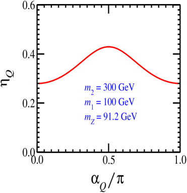
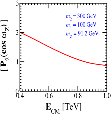
Figure 2: (Left) The coefficient $\eta_{\cal Q}$ is shown as a function of the phase $\alpha_{\cal Q}$. (Right) The integral $[P_{2}(\cos\omega_{{}_{Z}})]$ of the second Legendre polynomial $P_{2}$ of $\cos\omega_{{}_{Z}}$ is shown as a function of the $e^{-}e^{+}$ CM energy $\sqrt{s}=E_{\rm CM}$ (right). For this simple illustration, the range of $\sqrt{s}=E_{\rm CM}$ is taken to be from $0.4\,{\rm TeV}$ to $1.0\,{\rm TeV}$.

For an explicit numerical illustration, we set the following values for the $X_{2}$ and $X_{1}$ masses

$$m_{2}=300\,{\rm GeV}\quad\mbox{and}\quad m_{1}=100\,{\rm GeV}\,,$$ (52)

while varying the $e^{-}e^{+}$ CM energy $\sqrt{s}=E_{\rm CM}$ from 0.4 TeV to 1.0 TeV. The left side of Figure 2 shows the dependence of the coefficient $\eta_{\cal Q}$ on the phase $\alpha_{\cal Q}$. By measuring the coefficient we can determine the phase $\alpha_{\cal Q}$ up to a two-fold discrete ambiguity. Unless $\alpha_{\cal Q}$ is $0,\pi/2$ or $\pi$, i.e. unless ${\cal Q}$ is purely real or imaginary, CP is violated in the neutralino system. The right side of Figure 2 shows the integral of $P_{2}(\cos\omega_{{}_{Z}})=(3\cos^{2}\omega_{{}_{Z}}-1)/2$ over the polar angle $\theta_{Z}$ as a function of the $e^{-}e^{+}$ CM energy $\sqrt{s}=E_{\rm CM}$. For a simple illustration the $E_{\rm CM}$ range is taken from 0.4 TeV (identical to the threshold energy of $m_{2}+m_{1}$) to 1.0 TeV. The integral value is monotonically decreasing implying that the sensitivity to the complex factor ${\cal Q}$ is maximal at the production threshold. In contrast, the production cross section is increasing with the CM energy near the threshold. So, there exists a specific value of $E_{\rm CM}$ above the threshold for the optimal sensitivity to ${\cal Q}$.

5 Conclusions

In this paper we have made a general and systematic model-independent study of correlated distributions connected to the production process $e^{-}e^{+}\to X_{2}X_{1}$ of two Majorana particles $X_{2}$ and $X_{1}$ with different masses and arbitrary spins, followed by two sequential 2-body decays, $X_{2}\to ZX_{1}$ and $Z\to\ell^{-}\ell^{+}$ with $\ell=e$ or $\mu$, with invisible $X_{1}$. The constraints due to CP invariance and the Majorana condition were discussed. Formally, a proper Wick helicity rotation and an azimuthal-angle adjustment were taken into account for combining the production and decay helicity amplitudes derived in the most compact form from an analytic point of view and for describing a few general properties of the combined production-decay process involving two Majorana particles in a transparent way. Then, a specific example with the non-diagonal pair of two lighter neutralinos has been investigated for demonstrating the validity of all the worked-out general properties in a concrete and detailed manner.

In relation to this work we are at present analyzing the general structure of the $ZX_{2}X_{1}$ interaction vertices of a $Z$ boson and two Majorana particles $X_{2}$ and $X_{1}$ with any integer and/or half-integer spins and, furthermore, we plan to probe that of the interaction vertices of three Majorana particles with arbitrary spin combinations. This research project, of which the outcome will be reported soon elsewhere, is a natural extension of several previous works [38, 39, 40, 41, 42, 43].

References

• [1] S. L. Glashow, “Partial Symmetries of Weak Interactions,” Nucl. Phys. 22 (1961), 579-588 doi:10.1016/0029-5582(61)90469-2.
• [2] S. Weinberg, “A Model of Leptons,” Phys. Rev. Lett. 19 (1967), 1264-1266 doi:10.1103/PhysRevLett.19.1264.
• [3] A. Salam, “Weak and Electromagnetic Interactions,” Conf. Proc. C 680519 (1968), 367-377 doi:10.1142/9789812795915_0034.
• [4] G. Aad et al. [ATLAS], “Observation of a new particle in the search for the Standard Model Higgs boson with the ATLAS detector at the LHC,” Phys. Lett. B 716 (2012), 1-29 doi:10.1016/j.physletb.2012.08.020 [arXiv:1207.7214 [hep-ex]].
• [5] S. Chatrchyan et al. [CMS], “Observation of a New Boson at a Mass of 125 GeV with the CMS Experiment at the LHC,” Phys. Lett. B 716 (2012), 30-61 doi:10.1016/j.physletb.2012.08.021 [arXiv:1207.7235 [hep-ex]].
• [6] G. Aad et al. [ATLAS], “Combined measurements of Higgs boson production and decay using up to $80$ fb-1 of proton-proton collision data at $\sqrt{s}=$ 13 TeV collected with the ATLAS experiment,” Phys. Rev. D 101 (2020) no.1, 012002 doi:10.1103/PhysRevD.101.012002 [arXiv:1909.02845 [hep-ex]].
• [7] A. M. Sirunyan et al. [CMS], “Combined measurements of Higgs boson couplings in proton–proton collisions at $\sqrt{s}=13\,{\rm TeV}$,” Eur. Phys. J. C 79 (2019) no.5, 421 doi:10.1140/epjc/s10052-019-6909-y [arXiv:1809.10733 [hep-ex]].
• [8] M. C. Gonzalez-Garcia and M. Maltoni, “Phenomenology with Massive Neutrinos,” Phys. Rept. 460 (2008), 1-129 doi:10.1016/j.physrep.2007.12.004 [arXiv:0704.1800 [hep-ph]].
• [9] D. E. Morrissey and M. J. Ramsey-Musolf, “Electroweak baryogenesis,” New J. Phys. 14 (2012), 125003 doi:10.1088/1367-2630/14/12/125003 [arXiv:1206.2942 [hep-ph]].
• [10] W. Buchmuller, R. D. Peccei and T. Yanagida, “Leptogenesis as the origin of matter,” Ann. Rev. Nucl. Part. Sci. 55 (2005), 311-355 doi:10.1146/annurev.nucl.55.090704.151558 [arXiv:hep-ph/0502169 [hep-ph]].
• [11] G. Jungman, M. Kamionkowski and K. Griest, “Supersymmetric dark matter,” Phys. Rept. 267 (1996), 195-373 doi:10.1016/0370-1573(95)00058-5 [arXiv:hep-ph/9506380 [hep-ph]].
• [12] G. Bertone, D. Hooper and J. Silk, “Particle dark matter: Evidence, candidates and constraints,” Phys. Rept. 405 (2005), 279-390 doi:10.1016/j.physrep.2004.08.031 [arXiv:hep-ph/0404175 [hep-ph]].
• [13] M. Dine and A. Kusenko, “The Origin of the matter - antimatter asymmetry,” Rev. Mod. Phys. 76 (2003), 1 doi:10.1103/RevModPhys.76.1 [arXiv:hep-ph/0303065 [hep-ph]].
• [14] D. H. Lyth and A. Riotto, “Particle physics models of inflation and the cosmological density perturbation,” Phys. Rept. 314 (1999), 1-146 doi:10.1016/S0370-1573(98)00128-8 [arXiv:hep-ph/9807278 [hep-ph]].
• [15] E. Gildener and S. Weinberg, “Symmetry Breaking and Scalar Bosons,” Phys. Rev. D 13 (1976), 3333 doi:10.1103/PhysRevD.13.3333.
• [16] S. Weinberg, “Implications of Dynamical Symmetry Breaking,” Phys. Rev. D 13 (1976), 974-996 doi:10.1103/PhysRevD.19.1277.
• [17] L. Susskind, “Dynamics of Spontaneous Symmetry Breaking in the Weinberg-Salam Theory,” Phys. Rev. D 20 (1979), 2619-2625 doi:10.1103/PhysRevD.20.2619.
• [18] S. Y. Choi, J. Kalinowski, G. A. Moortgat-Pick and P. M. Zerwas, “Analysis of the neutralino system in supersymmetric theories,” Eur. Phys. J. C 22 (2001), 563-579 doi:10.1007/s100520100808 [arXiv:hep-ph/0108117 [hep-ph]].
• [19] S. R. Elliott and M. Franz, “Colloquium: Majorana Fermions in nuclear, particle and solid-state physics,” Rev. Mod. Phys. 87 (2015), 137 doi:10.1103/RevModPhys.87.137 [arXiv:1403.4976 [cond-mat.supr-con]].
• [20] S. Y. Choi, N. D. Christensen, D. Salmon and X. Wang, “Spin and chirality effects in antler-topology processes at high energy $e^{+}e^{-}$ colliders,” Eur. Phys. J. C 75 (2015) no.10, 481 doi:10.1140/epjc/s10052-015-3682-4 [arXiv:1503.02666 [hep-ph]].
• [21] S. Y. Choi, T. Han, J. Kalinowski, K. Rolbiecki and X. Wang, “Characterizing invisible electroweak particles through single-photon processes at high energy $e^{+}e^{-}$ colliders,” Phys. Rev. D 92 (2015) no.9, 095006 doi:10.1103/PhysRevD.92.095006 [arXiv:1503.08538 [hep-ph]].
• [22] E. Leader, “Spin in particle physics,” Camb. Monogr. Part. Phys. Nucl. Phys. Cosmol. 15 (2011), pp.1-500
• [23] S. Y. Choi, “$Z$-boson polarization as a model-discrimination analyzer,” Phys. Rev. D 98 (2018) no.11, 115037 doi:10.1103/PhysRevD.98.115037 [arXiv:1811.10377 [hep-ph]].
• [24] S. Y. Choi, J. H. Jeong and J. H. Song, “General Spin Analysis from Angular Correlations in Two-Body Decays,” Eur. Phys. J. Plus 135 (2020) no.2, 210 doi:10.1140/epjp/s13360-020-00132-1 [arXiv:1903.00166 [hep-ph]].
• [25] J. R. Ellis, J. M. Frere, J. S. Hagelin, G. L. Kane and S. T. Petcov, “Search for Neutral Gauge Fermions in $e^{+}e^{-}$ Annihilation,” Phys. Lett. B 132 (1983), 436-442 doi:10.1016/0370-2693(83)90343-X
• [26] S. M. Bilenky, N. P. Nedelcheva and E. K. Khristova, “On Production of Majorana Particles in Polarized $e^{+}e^{-}$ Collisions,” Phys. Lett. B 161 (1985), 397-399 doi:10.1016/0370-2693(85)90786-5
• [27] S. M. Bilenky, E. K. Khristova and N. P. Nedelcheva, “Possible Tests for Majorana Nature of Heavy Neutral Fermions Produced in Polarized $e^{+}e^{-}$ Collisions,” Bulg. J. Phys. 13 (1986), 283 JINR-E2-86-353.
• [28] G. A. Moortgat-Pick and H. Fraas, “Influence of CP and CPT on production and decay of Dirac and Majorana fermions,” Eur. Phys. J. C 25 (2002), 189-197 doi:10.1007/s10052-002-0979-x [arXiv:hep-ph/0204333 [hep-ph]].
• [29] E. K. Khristova and N. P. Nedelcheva, “On the Lightest Supersymmetric Particle in Polarized $e^{+}e^{-}$ Collisions,” Phys. Lett. B 208 (1988), 525-529 doi:10.1016/0370-2693(88)90661-2
• [30] A. B. Balantekin, A. de Gouvêa and B. Kayser, “Addressing the Majorana vs. Dirac Question with Neutrino Decays,” Phys. Lett. B 789 (2019), 488-495 doi:10.1016/j.physletb.2018.11.068 [arXiv:1808.10518 [hep-ph]].
• [31] G. C. Wick, “Angular momentum states for three relativistic particles,” Annals Phys. 18 (1962), 65-80 doi:10.1016/0003-4916(62)90059-3
• [32] M. E. Rose, “Elementary Theory of Angular Momentum” (Dover Publication Inc., New York, 2011) ISBN-13: 978-0486684802.
• [33] K. i. Hikasa, “Transverse Polarization Effects in $e^{+}e^{-}$ Collisions: The Role of Chiral Symmetry,” Phys. Rev. D 33 (1986), 3203 doi:10.1103/PhysRevD.33.3203
• [34] S. Y. Choi and Y. G. Kim, “Analysis of the neutralino system in two body decays of neutralinos,” Phys. Rev. D 69 (2004), 015011 doi:10.1103/PhysRevD.69.015011 [arXiv:hep-ph/0311037 [hep-ph]].
• [35] G. F. Giudice and A. Romanino, “Split supersymmetry,” Nucl. Phys. B 699 (2004), 65-89 [erratum: Nucl. Phys. B 706 (2005), 487-487] doi:10.1016/j.nuclphysb.2004.08.001 [arXiv:hep-ph/0406088 [hep-ph]].
• [36] N. Arkani-Hamed, S. Dimopoulos, G. F. Giudice and A. Romanino, “Aspects of split supersymmetry,” Nucl. Phys. B 709 (2005), 3-46 doi:10.1016/j.nuclphysb.2004.12.026 [arXiv:hep-ph/0409232 [hep-ph]].
• [37] P. A. Zyla et al. [Particle Data Group], “Review of Particle Physics,” PTEP 2020 (2020) no.8, 083C01 doi:10.1093/ptep/ptaa104
• [38] B. Kayser, “Majorana Neutrinos and their Electromagnetic Properties,” Phys. Rev. D 26 (1982), 1662 doi:10.1103/PhysRevD.26.1662
• [39] B. Kayser, “CPT, CP, and C Phases and their Effects in Majorana Particle Processes,” Phys. Rev. D 30 (1984), 1023 doi:10.1103/PhysRevD.30.1023
• [40] F. Boudjema, C. Hamzaoui, V. Rahal and H. C. Ren, “Electromagnetic Properties of Generalized Majorana Particles,” Phys. Rev. Lett. 62 (1989), 852 doi:10.1103/PhysRevLett.62.852
• [41] F. Boudjema and C. Hamzaoui, “Massive and massless Majorana particles of arbitrary spin: Covariant gauge couplings and production properties,” Phys. Rev. D 43 (1991), 3748-3758 doi:10.1103/PhysRevD.43.3748
• [42] J. F. Nieves and P. B. Pal, “Electromagnetic properties of neutral and charged spin 1 particles,” Phys. Rev. D 55 (1997), 3118-3130 doi:10.1103/PhysRevD.55.3118 [arXiv:hep-ph/9611431 [hep-ph]].
• [43] J. F. Nieves, “Electromagnetic properties of spin-3/2 Majorana particles,” Phys. Rev. D 88 (2013), 036006 doi:10.1103/PhysRevD.88.036006 [arXiv:1308.5889 [hep-ph]].