Sparse PCA via $\ell_{2,p}$-Norm Regularization
for Unsupervised Feature Selection

Abstract

In the field of data mining, how to deal with high-dimensional data is an inevitable problem. Unsupervised feature selection has attracted more and more attention because it does not rely on labels. The performance of spectral-based unsupervised methods depends on the quality of constructed similarity matrix, which is used to depict the intrinsic structure of data. However, real-world data contain a large number of noise samples and features, making the similarity matrix constructed by original data cannot be completely reliable. Worse still, the size of similarity matrix expands rapidly as the number of samples increases, making the computational cost increase significantly. Inspired by principal component analysis, we propose a simple and efficient unsupervised feature selection method, by combining reconstruction error with $\ell_{2,p}$-norm regularization. The projection matrix, which is used for feature selection, is learned by minimizing the reconstruction error under the sparse constraint. Then, we present an efficient optimization algorithm to solve the proposed unsupervised model, and analyse the convergence and computational complexity of the algorithm theoretically. Finally, extensive experiments on real-world data sets demonstrate the effectiveness of our proposed method.

1 Introduction

With the rapid development of information technology, high-dimensional data exist almost everywhere in all walks of life, such as weather forecast [1], financial transaction analysis [2], geological prospecting [3], image search [4], text mining [5], bioinformatics [6], etc. Unfortunately, the curse of dimensionality seriously restricts many practical applications. To solve this problem, feature selection is used to reduce the dimension by finding a relevant feature subset of data [7]. The advantages of feature selection mainly include: improving the performance of data mining tasks, reducing computational cost, improving the interpretability of data. Therefore, feature selection has become a necessary prerequisite for many data mining tasks, such as pattern recognition [8], clustering [9], classification [10], similarity retrieval [11], etc.

Based on whether data labels are available, feature selection can be divided into supervised and unsupervised methods [12]. Supervised feature selection utilizes the correlation between features and labels to find discriminative features. However, obtaining labels is expensive, or even impractical in many applications. Thus, unsupervised feature selection has attracted a lot of attention, because it does not rely on labels. In the paper, we propose a new method for unsupervised feature selection. The main contributions are summarized as follows:

• A new unsupervised model is proposed to perform feature selection. The sparse projection matrix is learned by minimizing the reconstruction error of data.

• An optimization algorithm is presented to solve the proposed model. We prove the convergence of the algorithm, and evaluate its computational complexity, which is linear to the number of samples.

• Extensive experiments on real-world data sets demonstrate the effectiveness of our proposed method.

The rest paper is organized as follows. In Section 2, we give a brief review of the related work and introduce some notations and definitions. In Section 3, we propose a new unsupervised feature selection model. In Section 4, the optimization algorithm is presented to solve the proposed model. In Section 5, we discuss the convergence and computational complexity of the optimization algorithm. In Section 6, experiments are implemented to evaluate the effectiveness of the proposed method. Finally, we provide the conclusion in Section 7.

2 Background

2.1 Related work

The techniques of unsupervised feature selection can be divided into three types [13]: filter, wrapper and embedded methods.

Filter methods [14] are independent of the data mining tasks. They are usually intuitive and computationally efficient. LapScore (Laplacian Score) [15] is one of the most classic filter methods. It calculates the score for each feature independently, according to its ability to preserve the intrinsic structure of original data. Then, all the features are ranked by the scores. Because each feature is evaluated independently, it may work well on binary-cluster problems, but are very likely to fail in multi-cluster cases [16].

Wrapper methods [17] combine feature selection with the data mining tasks. The mining algorithm is utilized to evaluate the effectiveness of selected features. The result of feature selection performs well in the mining task. However, wrapper methods are usually computationally expensive and weak in generalization.

Embedded methods [18] integrate feature selection into model learning. Since there is no need to evaluate feature subsets, they are more efficient than wrapper methods [19]. Thus, embedded methods have gradually become a hotspot, and many representative methods keep emerging, such as MCFS (Multi-Cluster Feature Selection) [16], UDFS (Unsupervised Discriminative Feature Selection) [20], EUFS (Embedded Unsupervised Feature Selection) [21], DGUFS (Dependence Guided Unsupervised Feature Selection) [22], SOGFS (Structured Optimal Graph Feature Selection) [23] and RNE (Robust Neighborhood Embedding Feature Selection) [24], etc.

MCFS selects features by using spectral regression with $\ell_{1}$-norm regularization, so that the multi-cluster structure of original data can be preserved. UDFS selects the discriminative features by joint discriminative analysis and $\ell_{2,1}$-norm minimization. EUFS embeds unsupervised feature selection into a clustering algorithm via sparse learning. $\ell_{2,1}$-norm is applied on the cost function to reduce the effects of noise. DGUFS enhances the interdependence among original data, cluster labels, and selected features. SOGFS conducts feature selection and local structure learning simultaneously, so that the similarity matrix can be determined adaptively. RNE selects features by calculating feature weight matrix through locally linear embedding algorithm, and ultilizing $\ell_{1}$-norm to minimize its reconstruction error.

Most embedded methods, even including LapScore, utilize spectral analysis and manifold learning to select discriminative features. They usually build a similarity matrix to depict the intrinsic structure of original data. However, real-world data contain a large number of noise samples and features, making the similarity matrix constructed by original data cannot be completely reliable. Worse still, the size of similarity matrix expands rapidly as the number of samples increases, making the computational cost increase significantly. Inspired by principal component analysis [25], we propose a simple and efficient unsupervised feature selection method from a new perspective.

2.2 Notations and definitions

We first introduce some notations and definitions that will be used throughout the paper. Given a matrix $M\in\mathbb{R}^{n\times d}$, the ($i,j$)-th element of $M$ is denoted by $m_{ij}$, its $i$-th row, $j$-th column are denoted by $m^{i}$, $m_{j}$ respectively. The transpose of $M$ is denoted by $M^{T}$. The trace of $M$ is denoted by ${\rm Tr}(M)$. The $\ell_{2,p}$-norm is defined as:

$$\begin{split}\left\|{\rm M}\right\|_{2,p}=\left(\sum_{i=1}^{n}{\left(\sum_{j=1}^{d}m_{ij}^{2}\right)}^{\frac{p}{2}}\right)^{\frac{1}{p}}=\left(\sum_{i=1}^{n}\left\|m^{i}\right\|_{2}^{p}\right)^{\frac{1}{p}},\ p>0\end{split}$$ (1)

When $p\geq 1$, since it satisfies the basic norm conditions, $\ell_{2,p}$-norm is a valid norm. However, when $0<p<1$, $\ell_{2,p}$ is not a valid norm. For convenience, we still call them norms in the paper.

3 Unsupervised feature selection model

Supposing a data set {$x_{1},x_{2},\ldots,x_{n}$} contains $n$ data points $x_{i}\in\mathbb{R}^{d\times 1}$, $X\in\mathbb{R}^{n\times d}$ denotes the data matrix. Without loss of generality, we assume that all the data points are centralized:

$$\begin{split}\sum_{i=1}^{n}x_{i}=0\end{split}$$ (2)

Supposing we explore principal component analysis for dimension reduction, the new coordinate system formed by principal components is:

$$\begin{split}&\{w_{1},w_{2},\ldots,w_{d}\},\quad w_{i}\in\mathbb{R}^{d\times 1}\\ &s.t.\quad\|w_{i}\|=1,\quad w^{T}_{i}w_{j}=0\ (i\neq j)\end{split}$$ (3)

If we want to reduce the dimension of the data points from $d$ to $m$ $(m<d)$, some coordinates in the coordinate system should be discarded. Then, the new coordinate system $W\in\mathbb{R}^{d\times m}$ is:

$$\begin{split}&W=\{w_{1},w_{2},\ldots,w_{m}\},\quad w_{i}\in\mathbb{R}^{d\times 1}\\ &s.t.\quad\|w_{i}\|=1,\quad w^{T}_{i}w_{j}=0\ (i\neq j)\end{split}$$ (4)

Thus, the projection of the data point $x_{i}$ in the new coordinate system is:

$$\begin{split}z_{i}=\{z_{i1},z_{i2},\ldots,z_{im}\}^{T},\quad z_{ij}=w^{T}_{j}x_{i}\end{split}$$ (5)

where $z_{ij}$ is the $j$th-dimension coordinate of $x_{i}$ in the low dimensional coordinate system. Eq. (5) can be rewritten as

$$\begin{split}z_{i}=W^{T}x_{i}\end{split}$$ (6)

If we reconstruct $x_{i}$ with $z_{i}$, the original data point can be recovered as:

$$\begin{split}\hat{x_{i}}=\sum_{j=1}^{m}{z_{ij}w_{j}}=Wz_{i}\end{split}$$ (7)

For the entire data set, the sum of the error between each original data point $x_{i}$ and its reconstructed point $\hat{x_{i}}$ is:

$$\begin{split}\sum_{i=1}^{n}\left\|\hat{x}_{i}-x_{i}\right\|_{2}^{2}\end{split}$$ (8)

We can substitute Eq. (7) into Eq. (8):

$$\begin{split}\sum_{i=1}^{n}\left\|Wz_{i}-x_{i}\right\|_{2}^{2}\end{split}$$ (9)

According to the property of $\ell_{2}$-norm, Eq. (9) can be further expanded to:

$$\begin{split}\sum_{i=1}^{n}\left(Wz_{i}\right)^{T}\left(Wz_{i}\right)-2\sum_{i=1}^{n}\left(Wz_{i}\right)^{T}x_{i}+\sum_{i=1}^{n}x_{i}^{T}x_{i}\end{split}$$ (10)

Due to $w^{T}_{i}w_{j}=0\ (i\neq j)$, we can get $W^{T}W=I$. Then, Eq. (10) can be converted to the following equation:

$$\begin{split}\sum_{i=1}^{n}z_{i}^{T}z_{i}-2\sum_{i=1}^{n}z_{i}^{T}W^{T}x_{i}+\sum_{i=1}^{n}x_{i}^{T}x_{i}\end{split}$$ (11)

According to Eq. (6), the above equation can be rewritten as

$$\begin{split}&\sum_{i=1}^{n}z_{i}^{T}z_{i}-2\sum_{i=1}^{n}z_{i}^{T}z_{i}+\sum_{i=1}^{n}x_{i}^{T}x_{i}\\ &=-\sum_{i=1}^{n}z_{i}^{T}z_{i}+\sum_{i=1}^{n}x_{i}^{T}x_{i}\end{split}$$ (12)

According to Eq. (2), Eq. (6) and the properties of matrix trace, we can get

$$\begin{split}\sum_{i=1}^{n}z_{i}^{T}z_{i}&=\operatorname{Tr}\left(W^{T}\left(\sum_{i=1}^{n}x_{i}x_{i}^{T}\right)W\right)\\ &=\operatorname{Tr}(W^{T}X^{T}XW)\end{split}$$ (13)

We can further substitute Eq. (13) into Eq. (12). Thus, Eq. (8) is equivalent to

$$\begin{split}-\operatorname{Tr}(W^{T}X^{T}XW)+\sum_{i=1}^{n}x_{i}^{T}x_{i}\end{split}$$ (14)

Principal component analysis requires that the reconstruction error should be minimal. Thus, the objective function is

$$\begin{split}\min_{W^{T}W=I}-\operatorname{Tr}(W^{T}X^{T}XW)+\sum_{i=1}^{n}x_{i}^{T}x_{i}\end{split}$$ (15)

For a given data set, $\sum_{i=1}^{n}x_{i}^{T}x_{i}$ is a constant, which has no impact on the minimization of the objective function. Then, Eq. (15) can be rewritten as

$$\begin{split}\min_{W^{T}W=I}-\operatorname{Tr}(W^{T}X^{T}XW)\end{split}$$ (16)

For the general case that the data points are not centralized, Eq. (16) can be rewritten as

$$\begin{split}\min_{W^{T}W=I}-\operatorname{Tr}(W^{T}S_{t}W)\end{split}$$ (17)

where $S_{t}=X^{T}HX$ is the total scatter matrix. $H$ is the centering matrix:

$$\begin{split}H=I_{n}-\frac{1}{n}\textbf{1}\textbf{1}^{T}\end{split}$$ (18)

As we all known, $\ell_{2,0}$-norm is the most suitable for feature selection. For the sake of feature selection, we add a regularization term to the objective function of Eq. (17):

$$\begin{split}&\min_{W^{T}W=I}-Tr(W^{T}S_{t}W)+\gamma\|W\|_{2,0}\end{split}$$ (19)

where $\gamma>0$ is a regularization parameter. The regularization term can make the projection matrix $W$ be sparse on the row vectors, so as to complete the task of feature selection. Unfortunately, it is difficult to solve $\ell_{2,0}$-norm problem directly. Because $\ell_{2,p}$-norm $(0<p\leq 1)$ is a reasonable choice to approximate $\ell_{2,0}$-norm in the feature selection task [23], we can replace $\ell_{2,0}$-norm with $\ell_{2,p}$-norm. Thus, Eq. (19) can be rewritten as

$$\begin{split}&\min_{W^{T}W=I}-Tr(W^{T}S_{t}W)+\gamma\|W\|_{2,p}^{p},\ 0<p\leq 1\end{split}$$ (20)

In the process of minimizing the objective function of Eq. (20), $\gamma\|W\|_{2,p}^{p}$ favors a small number of nonzero row vector $w^{i}$. The projection matrix $W$ should satisfy the following two constraints: it is sparse in the row vectors; the reconstruction error of all data points should be as small as possible, which is just the optimization direction of principal component analysis. For simplicity, we denote the proposed method as SPCAFS (Sparse Principal Component Analysis for Feature Selection).

4 Optimization algorithm

In this section, we present the optimization algorithm to solve problem (20). According to the definition of $\ell_{2,p}$-norm, problem (20) can be rewritten as

$$\begin{split}&\min_{W^{T}W=I}-\operatorname{Tr}(W^{T}S_{t}W)+\gamma\sum_{i=1}^{d}\left\|w^{i}\right\|_{2}^{p}\\ \end{split}$$ (21)

where $w^{i}\in\mathbb{R}^{m\times 1}$ is the $i$-th row vector of $W$. Since $\left\|w^{i}\right\|_{2}^{p}$ can be zero in theory, Eq. (21) may be non-differentiable. To avoid this case, we replace $\left\|w^{i}\right\|_{2}^{p}$ with $\left(w^{iT}w^{i}\right)^{\frac{p}{2}}$. Further, it is regularized as

$$\begin{split}\left(w^{iT}w^{i}\right)^{\frac{p}{2}}\rightarrow\left(w^{iT}w^{i}+\epsilon\right)^{\frac{p}{2}}\end{split}$$ (22)

where $\epsilon$ is a sufficiently small constant. Then, Eq. (21) can be equivalent to

$$\begin{split}&\min_{W^{T}W=I}-\operatorname{Tr}(W^{T}S_{t}W)+\gamma\sum_{i=1}^{d}\left(w^{iT}w^{i}+\epsilon\right)^{\frac{p}{2}}\end{split}$$ (23)

Theorem 1.

The solution to problem (23), i.e. $W\in\mathbb{R}^{d\times m}$, will contain at least $m$ non-zero rows.

Proof.

According to the constraint of problem (23), any feasible solution $W\in\mathbb{R}^{d\times m}$ should satisfy $W^{T}W=I_{m}$. Since $I_{m}\in\mathbb{R}^{m\times m}$, the rank of $W$ is $m$. Therefore, $W$ contains at least $m$ non-zero rows. ∎

The Lagrangian function of problem (23) is

$$\begin{split}\mathcal{L}(W,\Lambda)=&-\operatorname{Tr}(W^{T}S_{t}W)+\gamma\sum_{i=1}^{d}\left(w^{iT}w^{i}+\epsilon\right)^{\frac{p}{2}}\\ &+\operatorname{Tr}(\Lambda(W^{T}W-I))\end{split}$$ (24)

where $\Lambda$ is the Lagrangian multiplier. We take the derivative of Eq. (24) with respect to $W$, and set its value equal to zero. Then, we can get

$$\begin{split}\frac{\partial\mathcal{L}(W,\Lambda)}{\partial W}=&-S_{t}W+\gamma GW+W\Lambda=0\end{split}$$ (25)

where $G\in\mathbb{R}^{d\times d}$ is a diagonal matrix, and the $i$-th diagonal element is defined as

$$\begin{split}g_{ii}=\frac{p}{2}\left(w^{iT}w^{i}+\epsilon\right)^{\frac{p-2}{2}}\end{split}$$ (26)

It is worth noting that $G$ still depends on $W$. That is, $W$ cannot be directly calculated from Eq. (25). Thus, we utilize the following alternate optimization method to calculate $W$, $G$ iteratively.

Fix $G$ update $W$.

When $G$ is fixed, it is easily to prove that solving Eq. (25) is equivalent to solving

$$\begin{split}&\min_{W^{T}W=I}-\operatorname{Tr}(W^{T}S_{t}W)+\gamma\operatorname{Tr}(W^{T}GW)\end{split}$$ (27)

The optimal $W$ of Eq. (27) is formed by the $m$ eigenvectors of $(-S_{t}+\gamma G)$, corresponding to the $m$ smallest eigenvalues.

Fix $W$ update $G$.

When $W$ is fixed, we can easily calculate $G$ by Eq. (26).

Based on the above analysis, the optimization algorithm to solve problem (23) is summarized in Algorithm 1.

Algorithm 1 The algorithm to solve the problem (23).

0:  Data matrix $X\in\mathbb{R}^{n\times d}$, reduced dimension $m$, regularization parameter $\gamma$, a sufficiently small constant $\epsilon$.

0:  $h$ features of the data set.

1:  Initialize $S_{t}=X^{T}HX$ and $G=I$.

2:  repeat

3:     Update $W\in\mathbb{R}^{d\times m}$. The columns of $W$ are the $m$ eigenvectors of $(-S_{t}+\gamma G)$, corresponding to the $m$ smallest eigenvalues.

4:     Update $G$. The $i$-th element of $G$ is defined by Eq. (26).

5:  until converge

6:  Sort $\|w^{i}\|_{2}$ ($i=1,2,\dots,d$) in descending order, and select the top $h$ ranked features.

5 Discussion

5.1 Convergence analysis

The convergence of Algorithm 1 can guarantee that we can find a locally optimal solution of problem (23). Obviously, the converged solution satisfies KKT condition. To prove the convergence, we first introduce the following lemma. Please refer to [23] for the detailed proof.

Lemma 1.

When $0<p\leq 1$, for any positive real number $u$ and $v$, the following inequality holds:

$$\begin{split}u^{\frac{p}{2}}-\frac{p}{2}\frac{u}{v^{\frac{2-p}{2}}}\leq v^{\frac{p}{2}}-\frac{p}{2}\frac{v}{v^{\frac{2-p}{2}}}\end{split}$$ (28)

Theorem 2.

When we calculate $W$ according to Algorithm 1, updated $W$ will decrease the objective value of problem (23) until converge.

Proof.

Supposing the current updated $W$ is denoted by $\hat{W}$, we can easily derive the following inequality

$$\begin{split}&-\operatorname{Tr}(\hat{W}^{T}S_{t}\hat{W})+\gamma\operatorname{Tr}(\hat{W}^{T}G\hat{W})\leq\\ &-\operatorname{Tr}(W^{T}S_{t}W)+\gamma\operatorname{Tr}(W^{T}GW)\end{split}$$ (29)

We add the following item to the both sides of Eq. (29).

$$\begin{split}\gamma\sum_{i=1}^{d}\frac{p}{2}\frac{\epsilon}{\left(w^{iT}w^{i}+\epsilon\right)^{\frac{2-p}{2}}}\end{split}$$ (30)

Then, we can get

$$\begin{split}&-\operatorname{Tr}(\hat{W}^{T}S_{t}\hat{W})+\gamma\operatorname{Tr}(\hat{W}^{T}G\hat{W})+\sum_{i=1}^{d}\frac{\gamma p\epsilon}{2\left(w^{iT}w^{i}+\epsilon\right)^{\frac{2-p}{2}}}\leq\\ &-\operatorname{Tr}(W^{T}S_{t}W)+\gamma\operatorname{Tr}(W^{T}GW)+\sum_{i=1}^{d}\frac{\gamma p\epsilon}{2\left(w^{iT}w^{i}+\epsilon\right)^{\frac{2-p}{2}}}\end{split}$$ (31)

According to Eq. (26), we substitute $G$ into Eq. (31):

$$\begin{split}&-\operatorname{Tr}(\hat{W}^{T}S_{t}\hat{W})+\gamma\sum_{i=1}^{d}\frac{p}{2}\frac{\hat{w}^{iT}\hat{w}^{i}+\epsilon}{\left(w^{iT}w^{i}+\epsilon\right)^{\frac{2-p}{2}}}\leq\\ &-\operatorname{Tr}(W^{T}S_{t}W)+\gamma\sum_{i=1}^{d}\frac{p}{2}\frac{w^{iT}w^{i}+\epsilon}{\left(w^{iT}w^{i}+\epsilon\right)^{\frac{2-p}{2}}}\end{split}$$ (32)

Setting $u=\hat{w}^{iT}\hat{w}^{i}+\epsilon$, $v=w^{iT}w^{i}+\epsilon$, according to Lemma 1, we have the inequality:

$$\begin{split}&\left(\hat{w}^{iT}\hat{w}^{i}+\epsilon\right)^{\frac{p}{2}}-\frac{p}{2}\frac{\hat{w}^{iT}\hat{w}^{i}+\epsilon}{\left(w^{iT}w^{i}+\epsilon\right)^{\frac{2-p}{2}}}\leq\\ &\left(w^{iT}w^{i}+\epsilon\right)^{\frac{p}{2}}-\frac{p}{2}\frac{w^{iT}w^{i}+\epsilon}{\left(w^{iT}w^{i}+\epsilon\right)^{\frac{2-p}{2}}}\end{split}$$ (33)

Due to $\gamma>0$, we can further get

$$\begin{split}&\gamma\sum_{i=1}^{d}\left(\hat{w}^{iT}\hat{w}^{i}+\epsilon\right)^{\frac{p}{2}}-\gamma\sum_{i=1}^{d}\frac{p}{2}\frac{\hat{w}^{iT}\hat{w}^{i}+\epsilon}{\left(w^{iT}w^{i}+\epsilon\right)^{\frac{2-p}{2}}}\leq\\ &\gamma\sum_{i=1}^{d}\left(w^{iT}w^{i}+\epsilon\right)^{\frac{p}{2}}-\gamma\sum_{i=1}^{d}\frac{p}{2}\frac{w^{iT}w^{i}+\epsilon}{\left(w^{iT}w^{i}+\epsilon\right)^{\frac{2-p}{2}}}\end{split}$$ (34)

For Eq. (32) and Eq. (34), we add the left parts of the two inequalities. For the right parts, we perform the similar operation. Thus, we have

$$\begin{split}&-\operatorname{Tr}(\hat{W}^{T}S_{t}\hat{W})+\gamma\sum_{i=1}^{d}\left(\hat{w}^{iT}\hat{w}^{i}+\epsilon\right)^{\frac{p}{2}}\leq\\ &-\operatorname{Tr}(W^{T}S_{t}W)+\gamma\sum_{i=1}^{d}\left(w^{iT}w^{i}+\epsilon\right)^{\frac{p}{2}}\end{split}$$ (35)

By comparing Eq. (35) with problem (23), we can infer Theorem 2 holds. ∎

5.2 Computational complexity analysis

Since normalization is a prerequisite for all data mining tasks, we don’t count its computational cost into feature selection methods. The computational complexity of Algorithm 1 can be decomposed into the following aspects:

• We need $O(d^{2}n)$ to initialize $S_{t}$ and $G$, based on the normalized data.

• For one iteration, we need $O(d^{3})$ to update $W$ by performing eigen-decomposition of $(-S_{t}+\gamma G)$.

• For one iteration, we need $O(dm)$ to update $G$ according to Eq. (26).

• We need $O(dm)$ to calculate $\|w^{i}\|_{2}$ ($i=1,2,\dots,d$) and $O(d{\rm{log}}d)$ to complete the sorting.

Thus, the overall computational complexity is $O(d^{2}n+d^{3}t)$, where $t$ is the number of iterations of Algorithm 1. Note that, Algorithm 1 is efficient and always converges within 30 iterations in our experiments. We further compare its computational complexity in one iteration with that of other competing methods. In Table I, apart from some introduced notations, $c$ is the number of clusters, $p$ is the number of neighbours in graph construction, $h$ is the number of selected features. We can conclude that:

• For embedded methods, the computational complexity of sparse regression usually contains $d^{3}$, which is produced by inverse operation or eigen-decomposition.

• SPCAFS does not require the construction of a similarity matrix by KNN, which will need at least $O(dn^{2})$.

• Of all the methods, only the computational complexity of SPCAFS is linear to $n$. It indicates that the computational complexity of SPCAFS will not expand rapidly, as the number of samples increases.

TABLE I: Comparison of computational complexity.

Methods Computational complexity LapScore $O(dn^{2}+d{\rm{log_{2}}}d)$ MCFS $O(d^{3}+n^{2}m+d^{2}n)$ UDFS $O(d^{3}+n^{2}c)$ EUFS $O(dn^{2}+nc^{2})$ DGUFS $O(n^{3}+dn)$ SOGFS $O(d^{3}+n^{2}p+n^{2}c)$ RNE $O(dn^{2}+d^{2}n+d^{2}h)$ SPCAFS $O(d^{2}n+d^{3})$

6 Experimental evaluation

6.1 Experimental setup

6.1.1 Experimental environment and data sets

Hardware is a workstation with 3.8 GHz CPU and 16 GB RAM. The experimental environment is Windows 64-bit Operating System, running Matlab R2018a. Our experiments were executed on 6 publicly available data sets, including four image data sets PalmData25, Imm40, PIE and AR, two bioinformatics data sets SRBCTML and LEUML. More information of the data sets is shown in Table II.

TABLE II: The details of the experimental data sets.

Data sets # of Feature # of Instance # of Class PalmData25 256 2000 100 Imm40 1024 240 40 PIE 1024 1166 53 AR 2200 2600 100 SRBCTML 2308 83 4 LEUML 3571 72 2

6.1.2 Comparision methods and parameters setting

To verify the effectiveness of the proposed method, we compared it with several state-of-the-art methods in the field of unsupervised feature selection, such as LapScore, MCFS, UDFS, EUFS, DGUFS, SOGFS and RNE. To get the baseline for analysis, all features are selected as a special case of feature selection.

To ensure that the experiments are as fair as possible, we adopt the same strategy to set parameters for all the unsupervised feature selection methods. For LapScore, MCFS, UDFS, EUFS, DGUFS, SOGFS and RNE, we set the neighborhood size to be 5. For EUFS, SOGFS and SPCAFS, the reduced dimension is fixed as $m=c-1$. We tune all the parameters by grid search strategy from {$10^{-6},10^{-4},10^{-2},10^{0},10^{2},10^{4},10^{6}$ }. Without loss of generality, we set $p=1$ in $\ell_{2,p}$-norm regularization of SPCAFS.

6.1.3 Evaluation metrics

To verify the validity of SPCAFS, we execute $K$-means clustering by inputting the results of different unsupervised feature selection methods. Clustering accuracy (ACC) and Normalized Mutual Information (NMI) are utilized to evaluate the effectiveness of feature selection indirectly. ACC is defined as [26]

$$\begin{split}ACC=\frac{\sum_{i=1}^{n}\delta(c_{i},map(l_{i}))}{n}\end{split}$$ (36)

where $n$ is the number of data points, $c_{i}$ is the given cluster label, $l_{i}$ is the obtained cluster label, map(·) is the permutation mapping function that maps each obtained cluster label $l_{i}$ to the equivalent label from the data set. The best mapping can be found by using Kuhn–Munkres algorithm [27]. $\delta$ is a function defined as

$$\begin{split}&\delta(a,b)=\left\{{\begin{array}[]{l}1,\quad if\ a=b\\ 0,\quad otherwise\\ \end{array}}\right.\\ \end{split}$$ (37)

NMI is defined as [26]

$$\begin{split}NMI=\frac{MI(C,C^{\prime}))}{max(H(C),H(C^{\prime}))}\end{split}$$ (38)

where $C$ is the set of clusters obtained from the ground truth and $C^{\prime}$ is the set of clusters computed by a clustering algorithm. $MI(C,C)$ is the mutual information metric. $H(C)$, $H(C^{\prime})$ are the entropies of $C$ and $C^{\prime}$ respectively.

For each unsupervised feature selection method, the best result of $K$-means clustering with the optimal parameters is recorded. Since the result of $K$-means clustering depends on initialization, we repeated $K$-means clustering 20 times for all the methods, and report their average results.

6.2 Clustering results analysis with selected features

Without loss of generality, we set the number of selected features as {$10,20,30,40,50,60,70,80,90,100$ } for each data set. The experimental results of ACC, NMI are illustrated in Fig. 1, Fig. 2 respectively. We can get the following conclusions:

• Feature selection of SPCAFS is effective. Compared with the baseline (AllFea), both ACC and NMI of SPCAFS have been significantly improved on almost all these data sets. On PalmData25 data set, although ACC and NMI of SPCAFS are lower than the baseline, they are still higher than those of other methods. As the number of selected features increases, both ACC and NMI of SPCAFS gradually approach the baseline.

• In general, with the increase of the number of selected features, the curves of clustering results show a trend of rising first and then falling. Because data sets from practical applications usually contain many redundancy features and a few discriminative features. As the number of selected features increases, some redundancy features are selected, decreasing the clustering performance of feature selection methods.

• The performance of SPCAFS exceeds other competing methods on all these data sets. In particular on Imm40 data set, compared with the second best method MCFS, SPCAFS has 5 percent improvement of ACC, 3 percent improvement of NMI on average.

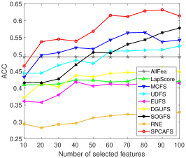
(a) Imm40

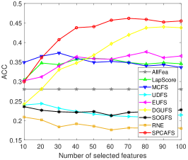
(b) PIE

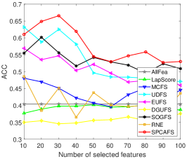
(c) SRBCTML

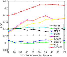
(d) AR

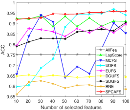
(e) LEUML

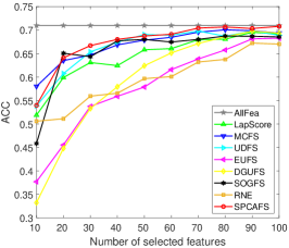
(f) PalmData25

Figure 1: Clustering results (ACC) of different unsupervised feature selection methods.

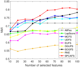
(a) Imm40

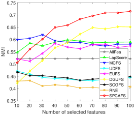
(b) PIE

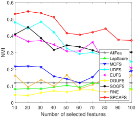
(c) SRBCTML

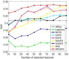
(d) AR

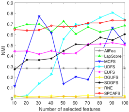
(e) LEUML

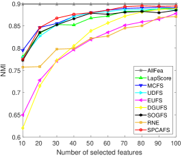
(f) PalmData25

Figure 2: Clustering results (NMI) of different unsupervised feature selection methods.

6.3 Convergence study

In Section 5.1, we have proven the convergence of Algorithm 1. We further study the speed of its convergence by experiments. The convergence curves of the objective value are demostrated in Fig. 3. Due to space limitation, we only show the results on four data sets. We can see that the speed of convergence of Algorithm 1 is very fast, which ensures the efficiency of SPCAFS.

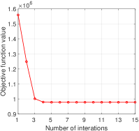
(a) PalmData25

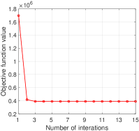
(b) Imm40

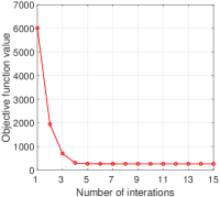
(c) SRBCTML

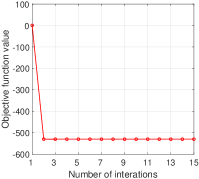
(d) LEUML

Figure 3: Convergence curve of SPCAFS on PalmData25, Imm40, SRBCTML and LEUML data sets.

6.4 Parameter sensitivity analysis

6.4.1 Sensitivity analysis for the parameters $\gamma$, $m$

We further investigate the impact of parameters $\gamma$, $m$ on SPCAFS. The experimental results on all these data sets are similar. Due to space limitation, we only present the experimental results on Imm40 data set. We first adjust $\gamma$ by fixing $m=c-1$. There are some small fluctuations in clustering performance under different $\gamma$, as illustrated in Fig. 4(a)-(b). Because $\gamma$ is used to control the row sparsity of projection matrix $W$, its variation will affect the result of feature selection. Then, we adjust $m$ by fixing $\gamma=10^{4}$. When $m$ changes from 10 to 70, the clustering performance does not change significantly, as illustrated in Fig. 4(c)-(d). The results indicate that SPCAFS is not sensitive to parameters $\gamma$ and $m$ with wide range, and it can be used in practical applications.

6.4.2 The effect of $p$ in $\ell_{2,p}$-Norm regularization

In the above experiments, we set $p=1$ in $\ell_{2,p}$-norm regularization by default. In this section, we discuss the effect of $p$ on the results of feature selection for SPCAFS. Without loss of generality, we only show the experimental results on Imm40, SRBCTML data sets, as illustrated in Fig. 5.

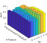
(a) ACC (m=39)

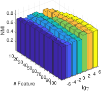
(b) NMI (m=39)

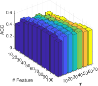
(c) ACC ($\gamma=10^{4}$)

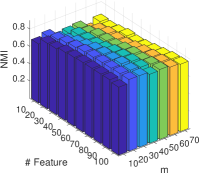
(d) NMI ($\gamma=10^{4}$)

Figure 4: ACC and NMI of SPCAFS under different $\gamma$, $m$ on Imm40 data set.

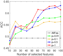
(a) Imm40 (ACC)

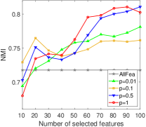
(b) Imm40 (NMI)

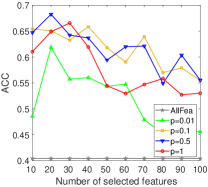
(c) SRBCTML (ACC)

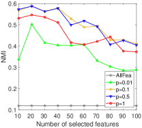
(d) SRBCTML (NMI)

Figure 5: ACC and NMI of SPCAFS under different $p$ on Imm40, SRBCTML data sets.

On Imm40 data set, when $p$ decreases from 1 to 0.1, the result of feature selection of SPCAFS becomes worse. On SRBCTML data set, as the value of $p$ decreases from 1 to 0.01, the results of feature selection show a trend of rising first and then falling. The phenomenon suggests that the choice of $p$ is not the smaller the better. The parameter $p$ is used to balance the sparsity and the convexity of the regularization. Small $p$ results in highly non-convex problem, which will increase the difficulty of optimization.

7 Conclusions

In the paper, we propose a new method for unsupervised feature selection, by combining reconstruction error with $\ell_{2,p}$-norm regularization. The projection matrix is learned by minimizing the reconstruction error under the sparse constraint. Then, we present an efficient optimization algorithm to solve the proposed unsupervised model, and analyse the convergence and computational complexity of the proposed algorithm. Finally, extensive experiments on real-world data sets demonstrate the effectiveness of our proposed method.

References

- [1] B. Ma and A. Entezari, “An interactive framework for visualization of weather forecast ensembles,” IEEE Transactions on Visualization and Computer Graphics, vol. 25, no. 1, pp. 1091–1101, 2019.
- [2] H. He, Y. Hong, W. Liu, and S. A. Kim, “Data mining model for multimedia financial time series using information entropy,” Journal of Intelligent and Fuzzy Systems, no. 1, pp. 1–7, 2020.
- [3] M. Dentith, R. J. Enkin, W. Morris, C. Adams, and B. Bourne, “Petrophysics and mineral exploration: a workflow for data analysis and a new interpretation framework,” Geophysical Prospecting, vol. 68, no. 1, pp. 178–199, 2020.
- [4] C. Deng, E. Yang, T. Liu, J. Li, W. Liu, and D. Tao, “Unsupervised semantic-preserving adversarial hashing for image search,” IEEE Transactions on Image Processing, vol. 28, no. 8, pp. 4032–4044, 2019.
- [5] F. Ali, S. El-Sappagh, and D. Kwak, “Fuzzy ontology and lstm-based text mining: A transportation network monitoring system for assisting travel,” Sensors, vol. 19, no. 2, 2019.
- [6] P. Luo, L. Tian, J. Ruan, and F. Wu, “Disease gene prediction by integrating ppi networks, clinical rna-seq data and omim data,” IEEE/ACM Transactions on Computational Biology and Bioinformatics, vol. 16, no. 1, pp. 222–232, 2019.
- [7] I. Guyon and A. Elisseeff, “An introduction to variable and feature selection,” Journal of Machine Learning Research, vol. 3, no. 6, pp. 1157–1182, 2003.
- [8] R. Zhang, J. Tao, and H. Zhou, “Fuzzy optimal energy management for fuel cell and supercapacitor systems using neural network based driving pattern recognition,” IEEE Transactions on Fuzzy Systems, vol. 27, no. 1, pp. 45–57, 2019.
- [9] A. Hoyos-Idrobo, G. Varoquaux, J. Kahn, and B. Thirion, “Recursive nearest agglomeration (rena): Fast clustering for approximation of structured signals,” IEEE Transactions on Pattern Analysis and Machine Intelligence, vol. 41, no. 3, pp. 669–681, 2019.
- [10] K. Kayabol, “Approximate sparse multinomial logistic regression for classification,” IEEE Transactions on Pattern Analysis and Machine Intelligence, vol. 42, no. 2, pp. 490–493, 2020.
- [11] Y. Wu, S. Wang, and Q. Huang, “Online fast adaptive low-rank similarity learning for cross-modal retrieval,” IEEE Transactions on Multimedia, vol. 22, no. 5, pp. 1310–1322, 2020.
- [12] L. Yu and H. Liu, “Eficient feature selection via analysis of relevance and redundancy,” Journal of Machine Learning Research, vol. 5, no. 12, pp. 1205–1224, 2004.
- [13] Z. Li, L. Jing, Y. Yi, X. Zhou, and H. Lu, “Clustering-guided sparse structural learning for unsupervised feature selection,” IEEE Transactions on Knowledge and Data Engineering, vol. 26, no. 9, pp. 2138–2150, 2014.
- [14] C. Lazar, “A survey on filter techniques for feature selection in gene expression microarray analysis,” IEEE/ACM Transactions on Computational Biology and Bioinformatics, vol. 9, no. 4, pp. 1106–1119, 2012.
- [15] X. He, D. Cai, and P. Niyogi, “Laplacian score for feature selection,” in Advances in Neural Information Processing Systems, 2005, pp. 507–514.
- [16] C. Deng, C. Zhang, and X. He, “Unsupervised feature selection for multi-cluster data,” in Acm Sigkdd International Conference on Knowledge Discovery and Data Mining, 2010, pp. 333–342.
- [17] M. M. Kabir, M. M. Islam, and K. Murase, “A new wrapper feature selection approach using neural network,” Neurocomputing, vol. 73, no. 16-18, pp. 3273–3283, 2008.
- [18] P. Chong, K. Zhao, Y. Ming, and C. Qiang, “Feature selection embedded subspace clustering,” IEEE Signal Processing Letters, vol. 23, no. 7, pp. 1018–1022, 2016.
- [19] J. Li, K. Cheng, S. Wang, F. Morstatter, R. P. Trevino, J. Tang, and H. Liu, “Feature selection: A data perspective,” Acm Computing Surveys, vol. 50, no. 6, pp. Article 39:1–45, 2016.
- [20] Y. Yang, H. Shen, Z. Ma, Z. Huang, and X. Zhou, “L21-norm regularized discriminative feature selection for unsupervised learning,” 07 2011, pp. 1589–1594.
- [21] S. Wang, J. Tang, and H. Liu, “Embedded unsupervised feature selection,” in Twenty-Ninth AAAI Conference on Artificial Intelligence, 2015, pp. 470–476.
- [22] J. Guo and W. Zhu, “Dependence guided unsupervised feature selection,” in Proceedings of the Thirty-Second AAAI Conference on Artificial Intelligence, New Orleans, Louisiana, USA, February 2-7, 2018. AAAI Press, 2018, pp. 2232–2239.
- [23] F. Nie, W. Zhu, and X. Li, “Structured graph optimization for unsupervised feature selection,” IEEE Transactions on Knowledge and Data Engineering, vol. PP, pp. 1–1, 08 2019.
- [24] Y. Liu, D. Ye, W. Li, and H. Wang, “Robust neighborhood embedding for unsupervised feature selection,” Knowledge-Based Systems, vol. 193, p. 105462, 04 2020.
- [25] I. T. Jolliffe, “Principal component analysis,” Journal of Marketing Research, vol. 87, no. 4, p. 513, 2002.
- [26] X. Zhu, S. Zhang, Y. Li, J. Zhang, L. Yang, and Y. Fang, “Low-rank sparse subspace for spectral clustering,” IEEE Transactions on Knowledge and Data Engineering, vol. 31, no. 8, pp. 1532–1543, 2019.
- [27] A. Strehl and J. Ghosh, “Cluster ensembles: a knowledge reuse framework for combining partitionings,” Journal of Machine Learning Research, vol. 3, no. 3, pp. 583–617, 2002.