Variation of Magnetic Flux Ropes Through Major Solar Flares

Abstract

It remains unclear how solar flares are triggered and in what conditions they can be eruptive with coronal mass ejections. Magnetic flux ropes (MFRs) has been suggested as the central magnetic structure of solar eruptions, and their ideal instabilities including mainly the kink instability (KI) and torus instability (TI) provide important candidates for triggering mechanisms. Here using magnetic field extrapolations from observed photospheric magnetograms, we systematically studied the variation of coronal magnetic fields, focusing on MFRs, through major flares including 29 eruptive and 16 confined events. We found that nearly 90% events possess MFR before flare and 70% have MFR even after flare. We calculated the controlling parameters of KI and TI, including the MFR’s maximum twist number and the decay index of its strapping field. Using the KI and TI thresholds empirically derived from solely the pre-flare MFRs, two distinct different regimes are shown in the variation of the MFR controlling parameters through flares. For the events with both parameters below their thresholds before flare, we found no systematic change of the parameters after the flares, in either the eruptive or confined events. In contrast, for the events with any of the two parameters exceeding their threshold before flare (most of them are eruptive), there is systematic decrease in the parameters to below their thresholds after flares. These results provide a strong constraint for the values of the instability thresholds and also stress the necessity of exploring other eruption mechanisms in addition to the ideal instabilities.

1 Introduction

Solar eruptions, often referred to explosive phenomena in the solar atmosphere, are leading driver of disastrous space weather. The two commonest forms of solar eruptions are solar flares and coronal mass ejections (CMEs), which are often closely related with each other (but not always). Both of them are believed to be caused by a drastic release of free energy stored in the complex, unstable magnetic field in the solar corona. Prediction of such eruptions is difficult since there are many important issues of the underlying physics remaining unresolved. For instance, the structure of the coronal magnetic field prior to eruption and the triggering mechanism of eruption are still undetermined; the key factor that causes the difference between eruptive flares (flares accompanied with CMEs) and confined flares (flares without CMEs) is still unclear.

Competing models of solar eruptions have been proposed based on either resistive magnetohydrodynamics (MHD), i.e., magnetic reconnection, or ideal MHD instabilities  (e.g., see reviews of Forbes et al., 2006; Shibata & Magara, 2011; Aulanier, 2014; Schmieder & Aulanier, 2012; Schmieder et al., 2013; Janvier et al., 2015). For example, in the reconnection-based models, such as the runaway tether-cutting reconnection (Moore et al., 2001) and the breakout reconnection (Antiochos et al., 1999), it is assumed that before the flare, the magnetic field has a strongly sheared configuration, and eruption is triggered by magnetic reconnection which is followed by a positive feedback between reconnection and outward expansion of the sheared magnetic flux. However, it is elusive to determine in what conditions the feedback can be established, and thus to develop prediction methods based on these models is not easy.

On the other hand, the ideal MHD instabilities, mainly the helical kink instability (KI, Hood & Priest, 1981; Török et al., 2004, 2010; Török & Kliem, 2005) and the torus instability (TI, Bateman, 1978; Kliem & Török, 2006) are developed based on magnetic flux rope (MFR, Kuperus & Raadu, 1974; Chen, 1989; Titov & Démoulin, 1999; Liu, 2020), which is a coherent group of twisted magnetic flux winding around a common axis. In the MFR-based models, it is assumed that MFR exists in the corona prior to eruption. Then the pre-existing MFR is slowly driven to an unstable regime by motions in the lower atmosphere (the photosphere), and is triggered to erupt through either KI or TI. The twist degree of the MFR itself and the decay index of the MFR’s strapping field (Török & Kliem, 2005, 2007; Kliem & Török, 2006) are two critical parameters which control the KI and TI, respectively, and instabilities occur when they exceeds some values, i.e., the instability thresholds. Thus, the controlling parameters of the instabilities can be used potentially in forecasting solar eruptions, which is a unique advantage of the ideal MHD models, and to this end, it is crucial to identify the MFRs in the coronal magnetic field and to precisely determine the thresholds of the instabilities.

However, there appears to be no single value for the thresholds, and different studies, from either analytic, numerical or even laboratory investigations, often give out discrepant results. For instance, the KI threshold $T_{w}$, which measures the winding number of magnetic field lines around the MFR’s axis, is found to range from $\sim 1.25$ turns to $\sim 2.5$ turns in previous analytic and numerical investigations (Hood & Priest, 1981; Baty, 2001; Fan & Gibson, 2003; Török & Kliem, 2003, 2005) because it depends on the details of the MFR, such as the line-tying effects by the photosphere, the aspect ratio of the MFR (i.e., ratio of the rope’s length to its cross-section size), and the geometry of the axis. The TI controlling parameter, i.e., the decay index $n$, refers to the spatial decreasing speed of the MFR’s overlying magnetic field that straps the MFR. A series of theoretical and numerical studies (Kliem & Török, 2006; Török & Kliem, 2007; Fan & Gibson, 2007; Aulanier et al., 2010; Démoulin & Aulanier, 2010; Fan, 2010; Zuccarello et al., 2015) show that the TI threshold of decay index has typical values in the domain of $1.1\sim 2$, while some laboratory experiments suggest that it might be much lower as being $0.65\sim 1.1$ (Myers et al., 2015; Alt et al., 2020), depending mainly on the ratio of the apex height and footpoint half-separation.

Furthermore, due to the intrinsic complexity of the magnetic field in the solar corona, the configuration of MFRs can be very different from case to case, which may not be fully characterized by the KI and TI theories that are derived based on relatively simplified or idealized configuration in the previous analytic, numerical and laboratory investigations. In some cases, if the filaments have significant rotational motions, they tend to be associated with failed eruptions despite the decay index satisfying the threshold for torus instability (Zhou et al., 2019). Recently, statistical studies based on magnetic field extrapolation have been employed to study configurations of coronal MFRs focusing on the two controlling parameters, in the hope of finding more realistic thresholds that can be used for prediction and to differentiate the types of eruptive and confined flares. Using a nonlinear-force-free field (NLFFF) extrapolation code developed by Wiegelmann (2004) based on the optimization method, Jing et al. (2018) surveyed the pre-flare coronal magnetic field for 38 major flares, and they found that only the TI plays an important role in distinguishing the different types of flares, with the threshold of decay index found to be $\sim 0.75$, which is much lower than the canonical value of $1.5$ (Kliem & Török, 2006). The twist numbers show no systematic difference between the confined and eruptive events. Then, Duan et al. (2019) performed a similar survey of 45 major flares with the pre-flare force-free magnetic field reconstructed by another NLFFF extrapolation method, the CESE–MHD–NLFFF code, which is based on the MHD-relaxation method (Jiang & Feng, 2013). They used a more strict definition of MFR which refers to field lines with winding number of at least one full turn, and found that $\sim 90$% of the events possess pre-flare MFRs but with very different three-dimensional structures. Quite different from the results in Jing et al. (2018), the newer study found the KI and TI thresholds to be $|T_{w}|_{\rm crit}\sim 2$ and $n_{\rm crit}\sim 1.3$, respectively, which are close to values derived in theoretical studies, and KI and TI play a nearly equally important role in discriminating the eruptive and confined flares.

The two previous studies have only analyzed the pre-flare magnetic fields. In this Letter, we investigate for the first time the variations of MFRs, focusing on changes of the two controlling parameters of KI and TI, from immediately pre-flare to post-flare states. For comparison, we use the same events studied in Duan et al. (2019) and thus the CESE–MHD–NLFFF code is employed to reconstruct both the pre-flare and post-flare coronal magnetic fields. It is found that the existences of post-flare MFR are also very common, even for the eruptive flares, suggesting that the pre-flare MFR often does not expel out entirely. Furthermore, a key difference of the variation of the controlling parameters from before to after flare is shown in two different regimes of events defined by the KI and TI thresholds derived in our previous study. These results provide a strong constraint for the values of the instability thresholds, and confirm that the events with pre-flare parameters exceeding the thresholds are very likely triggered by the ideal instabilities, while for those with the two parameters below the thresholds, which account for more than half of all the events, other mechanisms such as the reconnection-based ones should be considered.

Table 1: List of events and parameters of their pre- and post-flare MFRs.

No.	Flare peak time	Flare class	NOAA AR	Position	E/Ca	$T_{w}$ beforeb	$n$ before	$T_{w}$ afterc	$n$ after
1	SOL2011-02-13T17:38	M6.6	11158	S20E04	E	0.76	0.99	0.55	1.25
2	SOL2011-02-15T01:56	X2.2	11158	S20W10	E	1.52	0.98	0.86	0.69
3	SOL2011-03-09T23:23	X1.5	11166	N08W09	C	-1.75	0.50	-1.45	0.30
4	SOL2011-07-30T02:09	M9.3	11261	S20W10	C	-0.88	0.51	-0.80	1.48
5	SOL2011-08-03T13:48	M6.0	11261	N16W30	E	2.45	1.40	1.68	1.14
6	SOL2011-09-06T01:50	M5.3	11283	N14W07	E	0.92	0.52	1.30	0.40
7	SOL2011-09-06T22:20	X2.1	11283	N14W18	E	1.02	1.65	0.89	0.17
8	SOL2011-10-02T00:50	M3.9	11305	N12W26	C	-0.92	0.42	-0.92	0.20
9	SOL2012-01-23T03:59	M8.7	11402	N28W21	E	-1.63	0.73	-1.40	1.17
10	SOL2012-03-07T00:24	X5.4	11429	N17E31	E	-2.11	0.71	-1.96	0.98
11	SOL2012-03-09T03:53	M6.3	11429	N15W03	E	-1.17	0.73	-1.38	0.61
12	SOL2012-05-10T04:18	M5.7	11476	N12E22	C	-1.11	1.21	-0.77	1.11
13	SOL2012-07-02T10:52	M5.6	11515	S17E08	E	-1.56	0.35	-1.25	0.15
14	SOL2012-07-05T11:44	M6.1	11515	S18W32	C	1.14	-0.41	1.14	-0.03
15	SOL2012-07-12T16:49	X1.4	11520	S15W01	E	2.20	0.42	1.83	0.28
16	SOL2013-04-11T07:16	M6.5	11719	N09E12	E	-1.10	0.26	-2.00	0.09
17	SOL2013-10-24T00:30	M9.3	11877	S09E10	E	2.00	0.56	1.50	0.42
18	SOL2013-11-01T19:53	M6.3	11884	S12E01	C	1.50	0.42	1.60	1.40
19	SOL2013-11-03T05:22	M4.9	11884	S12W17	C	3.00	0.07	2.10	0.27
20	SOL2013-11-05T22:12	X3.3	11890	S12E44	E	1.35	2.72	1.10	1.57
21	SOL2013-11-08T04:26	X1.1	11890	S12E13	E	1.26	1.87	0.80	0.49
22	SOL2013-12-31T21:58	M6.4	11936	S15W36	E	-2.20	1.11	-1.65	0.67
23	SOL2014-01-07T10:13	M7.2	11944	S13E13	C	1.65	0.21	0.88	0.39
24d	SOL2014-01-07T18:32	X1.2	11944	S15W11	E	6.50	0.20	3.86	0.31
25	SOL2014-02-02T09:31	M4.4	11967	S10E13	C	-1.73	-0.12	-1.81	-0.04
26	SOL2014-02-04T04:00	M5.2	11967	S14W06	C	-1.90	1.03	-1.68	0.96
27	SOL2014-03-29T17:48	X1.1	12017	N10W32	E	1.53	1.72	0.60	1.37
28	SOL2014-04-18T13:03	M7.3	12036	S20W34	E	2.30	1.82	1.60	0.49
29	SOL2014-09-10T17:45	X1.6	12158	N11E05	E	-0.85	0.17	-1.31	0.16
30d	SOL2014-09-28T02:58	M5.1	12173	S13W23	E	-2.76	1.96	-2.00	0.57
31	SOL2014-10-22T14:28	X1.6	12192	S14E13	C	-1.10	0.94	-0.99	0.91
32	SOL2014-10-24T21:41	X3.1	12192	S22W21	C	-1.79	0.64	-1.55	0.50
33	SOL2014-11-07T17:26	X1.6	12205	N17E40	E	3.55	1.21	1.60	0.51
34	SOL2014-12-04T18:25	M6.1	12222	S20W31	C	2.60	0.60	1.86	0.65
35	SOL2014-12-17T04:51	M8.7	12242	S18E08	E	0.70	0.66	0.71	0.58
36	SOL2014-12-18T21:58	M6.9	12241	S11E15	E	1.09	1.49	1.00	0.27
37	SOL2014-12-20T00:28	X1.8	12242	S19W29	E	1.32	0.56	1.18	0.53
38	SOL2015-03-11T16:21	X2.1	12297	S17E22	E	2.04	1.80	1.29	0.51
39	SOL2015-03-12T14:08	M4.2	12297	S15E06	C	1.10	0.72	1.30	0.99
40	SOL2015-06-22T18:23	M6.5	12371	N13W06	E	-1.24	1.51	-0.93	1.37
41	SOL2015-06-25T08:16	M7.9	12371	N12W40	E	-2.90	0.49	-2.10	0.56
42	SOL2015-08-24T07:33	M5.6	12403	S14E00	C	1.04	0.33	0.73	0.36
43	SOL2015-09-28T14:58	M7.6	12422	S20W28	C	-1.25	1.20	-1.25	1.06
44	SOL2017-09-04T20:33	M5.5	12673	S10W11	E	-1.43	1.09	-1.45	0.49
45	SOL2017-09-06T12:02	X9.3	12673	S09W34	E	-1.80	1.72	-1.10	0.22

2 Data and Method

We have investigated 29 eruptive flares (above GOES-class M5) and 16 confined ones (above M3.9) observed by the Solar Dynamic Observatory (SDO, Pesnell et al., 2012) from 2011 January to 2017 December, which are listed in Table 1. All the 45 events occurred within $45^{\circ}$ in longitude of the disk center, and most of them are active region (AR) flares  (see more details of the criterion for selecting events in Duan et al., 2019). Based on the vector magnetograms from the Helioseismic and Magnetic Imager (HMI, Hoeksema et al., 2014) onboard SDO, the CESE–MHD–NLFFF code (Jiang & Feng, 2013) was used to reconstruct a pre-flare 3D coronal magnetic field and a post-flare one for each event. For the pre-flare reconstruction, we used the last available data for at least 10 minutes before the flare start time to avoid the possible artifacts introduced by the strong flare emission, while for the post-flare field, we used the first available magnetogram at least 1 hour after the flare peak, a time when the post-flare field relaxed to nearly MHD equilibrium but without significant further stressing by the photospheric motions. The vector magnetograms are obtained from the Space-weather HMI Active Region Patch (SHARP, Bobra et al., 2014) data product.

Following the same procedure introduced in Duan et al. (2019), we first search for MFRs in the full reconstruction volume based on the volumetric distribution of the magnetic twist number $T_{w}$ (Berger & Prior, 2006), which can provide a good approximation of the winding turns of two infinitesimally close field lines about each other. $T_{w}$ is defined for closed field lines (whose two footpoints are anchored in the photosphere) as

$$T_{w}=\int_{L}\frac{(\nabla\times{\mathbf{B}})\cdot{\mathbf{B}}}{4\pi B^{2}}dl$$ (1)

where the integral is taken along the field lines. We calculate $T_{w}$ on grid points with a resolution of 4 times of the original data, and define the MFR as a coherent group of magnetic field lines with $T_{w}$ of the same sign and $|T_{w}|\geq 1$. Thus an MFR approximately has all field lines with winding around the axis at least one full turn, which is a strict definition. Moreover, the MFRs as found with the $T_{w}$ distribution are further selected by restricting them within the flare sites, e.g., through comparing with SDO/AIA observable filaments and flare ribbons in the flare site. One may refer to Duan et al. (2019) for more information about the definition and selection of MFRs. Both Liu et al. (2016) and Duan et al. (2019) suggested that the maximum value of $|T_{w}|$ can be regarded as a reliable proxy of the MFR axis, and they also pointed out that the $|T_{w}|_{\rm max}$ has a very sensitive association with KI occurring in flares. Thus we employ the $|T_{w}|_{\rm max}$ as the KI controlling parameter .

As aforementioned, TI is controlled by the decay index of the strapping field of the MFR. In many literatures, the decay index is simply defined as along the vertical or radial direction. However, nonradial eruptions are frequently observed in filament eruptions (McCauley et al., 2015). Thus, in this Letter, the decay index is calculated along an oblique line matching the direction of the eruption. In a configuration where the MFR significantly deviates from the vertical direction, we use a slice cutting through the middle of the rope axis (often at its apex, marked as P) perpendicularly, and the slice intersects with the bottom polarity inversion line (PIL) on the point marked as O. OP is the oblique line directing from O to P. The strapping magnetic field is extrapolated from the $B_{z}$ component of the photospheric magnetogram with the potential field model. Then, it is decomposed into three orthogonal components $B_{\rm e}$, $B_{\rm p}$ and $B_{\rm t}$, where $B_{\rm e}$ is along OP, $B_{\rm p}$ is perpendicular to the OP on the slice, and $B_{\rm t}$ is perpendicular to the slice (one can refer to Figure 2 in Duan et al., 2019). Among them, only the cross product between the current of the rope and the poloidal flux $B_{\rm p}$ can produce an effective strapping force directing P to O, since $B_{\rm t}$ is parallel to the current of the rope, and the cross product of the current with $B_{\rm e}$ produces a force parallel to $B_{\rm p}$ which can only control the eruption direction, besides, $B_{\rm e}$ often has a small value. Thus, to be more relevant, we define the decay index $n$ as

$$n=\frac{d\log(B_{\rm p})}{d\log(r)}$$ (2)

where $r$ is the distance pointing from O to P.

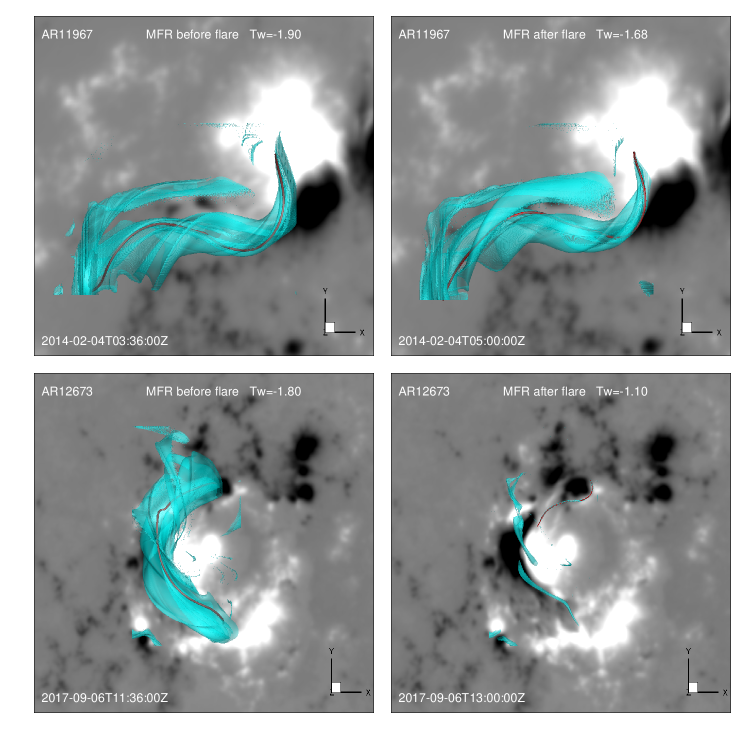
Figure 1: Two examples showing the MFRs before (left) and after (right) flares. The top panels show the results for an M5.2 confined flare (event 26) on 2014 February 4 in AR 11967. The bottom panels show results for an X9.3 eruptive flare (event 45) on 2017 September 6 in AR 12673. In all the panels, the cyan, transparent 3D object is the isosurface of the $|T_{w}|$ = 1, showing the surface of MFRs. Embedded in the isosurface is axis of the MFR which is denoted by the red, thick line. The MFR axis possesses the maximum of $|T_{w}|$ which is denoted on each panel. The background images show the magnetic flux distribution on the photosphere with the positive flux colored in white and negative flux in black.

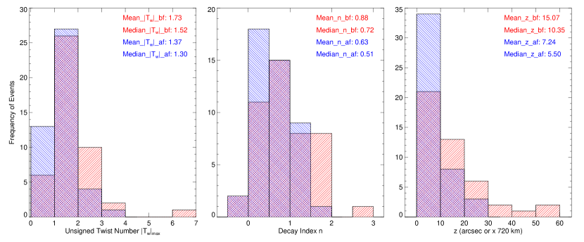
Figure 2: Histogram of the twist number $|T_{w}|_{\max}$, the decay index $n$ and the apex height of magnetic field rope axis $z_{\max}$. The red and blue boxes denote before and after flares, respectively. The average and median values for all the parameters are denoted in each panel.

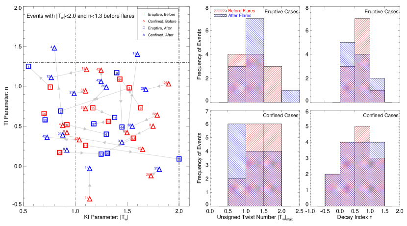
Figure 3: Left: Scatter diagram of decay index $n$ (TI parameter) vs. $|T_{w}|_{\rm max}$ (KI parameter) for events with $|T_{w}|<2.0$ and $n<1.3$ before flares. The boxes (triangles) denote eruptive (confined) flares, while red (blue) color denotes before (after) flares, and number of the events is marked within or neighboring to the boxes and triangles; also see the gray arrows pointing from before to after the flares. The thick dashed lines show $|T_{w}|=2$ and the $n=1.3$, i.e., the empirically derived thresholds, while the thin dashed line show $|T_{w}|=1$, below which the MFR does not exist. Right: Histogram of the twist number $|T_{w}|_{\max}$ and the decay index $n$ before and after flares for the two types of flares.

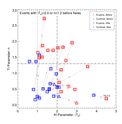
Figure 4: Same as the left panel of Figure 3, but for events with $|T_{w}|\geq 2$ or $n\geq 1.3$ before flares. Note that the pre-flare $|T_{w}|$ for event 24 is $6.5$, and we show here $(|T_{w}|-2.0)$ for a better display of the plot.

3 Results

Our previous survey (Duan et al., 2019) basing on only the pre-eruption magnetic fields found that 39 of the 45 events possess pre-flare MFRs and suggested that the lower limits for TI and KI thresholds are $n_{\rm crit}=1.3$ and $|T_{w}|_{\rm crit}=2$, respectively, since 90% of events (11 in 13 events) with $|T_{w}|\geq 2$ erupted and all events (11 events) with $n\geq 1.3$ erupted. Thus, it seems that KI and TI play a nearly equally important role in discriminating the eruptive and confined flares. Here we focus on how two parameters change from before to after eruptions.

Before showing the statistical results, we first give two typical examples of the variation of MFR through two flares, as shown in Figure 1. The first one is the event 26 in Table 1, an M5.2 confined flare on 2014 February 4 in AR 11967. The MFR before the flare has a coherent structure with peak twist number of $T_{w}=-1.9$ (see the pre-flare MFR configurations for all the studied events in Duan et al., 2019), and after the flare it shows no evident change with the peak twist number only slightly reduced to $T_{w}=-1.68$. The decay index at the apex of the MFR is $n=1.03$ before the flare and $n=0.96$ after. The small variation of the MFR through the flare is consistent with the confining nature of the flare. The second example is shown for event 45, an X9.3 eruptive flare on 2017 September 6 in AR 12673. As shown in Figure 1, before the flare, there is a thick, long MFR with peak twist number of $T_{w}=-1.8$, and it displays a good coherence and runs roughly along the main PIL of the AR. After an X9.3 flare, the MFR disintegrated, leaving a much thinner MFR with rather weak peak twist of $T_{w}=-1.1$, indicating that most (but not all) of the pre-flare twisted flux of the MFR erupted during the flare in this case. The remaining MFR after the flare is much lower than the pre-flare one, and thus the decay index $n$ drops from $1.72$ to $0.22$. This is a clear example in which both the twist number and the decay index of the MFR decrease significantly through the eruption.

In Table 1, we list the parameters for all the events including the pre-flare peak $T_{w}$ and $n$ and their post-flare values. Figure 2 shows histograms for the distributions of the two parameters, $|T_{w}|_{\max}$ and $n$, as well as the apex height of MFR axis in all the events before and after flares. As can be seen, on average all the parameters show decrease through flares; the average $|T_{w}|_{\max}$ decreases from $1.73$ to $1.37$; the average $n$ decreases from $0.88$ to $0.63$, and the average apex height of MFRs is lowered from $15$ arcsec to $7$ arcsec. We note that, as shown in the $|T_{w}|_{\max}$ distribution, a majority of the events (32 in 45, or 71%, which is comparable to the pre-flare percent of 87%) after flare still have MFR using our strict definition (i.e., magnetic flux with $|T_{w}|>1$), suggesting that MFR existing after flares is rather common.

Figures 3 (left panel) and 4 show the scatter diagrams of decay index $n$ versus $|T_{w}|_{\max}$ in two regimes for a better inspection. Specifically, in Figure 3, we show all the events with $|T_{w}|_{\max}<2.0$ and $n<1.3$ before flares, which are below the thresholds ($|T_{w}|_{\rm crit}$ and $n_{\rm crit}$) empirically derived in our previous survey (Duan et al., 2019) and thus are not likely triggered by the ideal instabilities. There are in total 25 events (14 confined and 11 eruptive) in this regime of parameter space. From the overall change of the pre-flare values (colored in red) to their post-flare ones (colored in blue) of the two parameters, one can see the events distribute rather randomly in the region bounded by $0<n<1.3$ and $0.5<|T_{w}|<2$ without a systematic decrease in either the twist number or the decay index. There are only two confined events, i.e., event 4 and 18, in which the post-flare decay index $n$ increases to above the threshold slightly. In the right panels of Figure 3, we show the histograms of the two parameters before and after flares for the two types of events separately. Again there is no systematic difference between the eruptive and confined flares, indicating that the two parameters and its changes are unable to discriminating the type of flares if both of them are lower than the thresholds. This is consistent with the conclusion in Duan et al. (2019) that the triggering mechanisms of the events fall in this domain of the parameter space are not related with the ideal instabilities.

In contrast, Figure 4 shows the events with pre-flare $|T_{w}|_{\max}\geq 2.0$ or $n\geq 1.3$, namely, the ones with pre-flare KI or TI parameter (in some cases like events 5, 28, 30 and 38 both KI and TI parameters) exceeding their thresholds. In this domain of parameter space, we have in total 20 events in which 18 are eruptive. Very clear and distinct from the distributions in Figure 3 (left panel), we can see that these events show systematic decrease in either $|T_{w}|_{\max}$ or $n$ from through flares. Furthermore, in most of the events (18 in 20, or 90% of the events), both parameters after flares decrease to close to or lower than their thresholds, i.e., most of the blue marks as seen in the figure concentrate on the lower left quadrant with $n<1.3$ and $T_{w}<2$, except event 20 and 24. These results, again, are highly consistent with and support our previous statistics (Duan et al., 2019), i.e., the thresholds for KI and TI parameters ($|T_{w}|_{max}\geq 2.0$ and $n\geq 1.3$) are reasonable, and these events are very likely triggered by the ideal instabilities. It is also worthy noting that the most of the eruptive events have MFR after flares by our strict definition (i.e., with $|T_{w}|>1$), which indicates that the pre-flare MFR often does not expel out entirely during eruption.

4 Summary

In this Letter, we systematically studied the coronal magnetic field changes, focusing on MFRs, before and after solar flares for 45 major flare events, including 29 eruptive ones and 16 confined ones. Using the CESE–MHD–NLFFF method with SDO/HMI vector magnetograms as input, we reconstructed the coronal magnetic fields immediately prior to and after the flares for all events. Then we searched the MFR for each event using a strict definition of MFR based on 3D distribution of magnetic twist number (i.e., MFR must have a coherent groud of magnetic flux with twist number of $|T_{w}|\geq 1$ of constant sign), and found that while most events possess pre-flare MFRs, the post-flare MFRs are also very common in a high percent (71%) of the events. Furthermore, we calculated the two controlling parameters of ideal MHD instabilities of MFR, i.e., the maximum twist number $|T_{w}|_{\max}$, which controls KI, and the decay index $n$ of the strapping field which controls TI. For all the events, the average values for the two parameters show decrease from before to after flares, with the average $|T_{w}|_{\max}$ decreases from $1.73$ to $1.37$ and the average $n$ decreases from $0.88$ to $0.63$, indicating of magnetic twist releasing and MFR height decreasing through flares.

A key difference of the variation of the two parameters from before to after flare is shown in the two different regimes defined by the KI and TI thresholds derived in our previous study (Duan et al., 2019), which are $|T_{w}|_{\rm crit}=2$ and $n_{\rm crit}=1.3$, respectively. For the events with both parameters before flares below their thresholds, most of them after flares are also lower than their thresholds, without systematic change of the parameters found from before to after the flares, and the two parameters and their changes are unable to discriminating the eruptive or confined type of flares. While for the events with any of the two parameters exceeding their threshold before flare, there is systematic decrease in either $|T_{w}|_{\max}$ or $n$ after flare, and in most of these events, both parameters decrease to close to or lower than their thresholds. Thus the pre-flare to post-flare changes of the two parameters confirm our empirically derived thresholds for KI and TI (i.e., $|T_{w}|_{\rm crit}=2$ and $n_{\rm crit}=1.3$), above which these events are very likely triggered by the ideal instabilities and can be eruptive. While for those with the two parameters below the thresholds, other eruption mechanisms such as the reconnection-based ones should be considered to understand the triggering of the flares and the conditions determining the eruptive or confined types. These results give a strong constraint for the values of the instability thresholds and also stress the necessity of exploring other eruption mechanisms in addition to the ideal MHD instabilities.

References

- Alt et al. (2020) Alt, A., Myers, C. E., Ji, H., et al. 2020, arXiv:2010.10607 [astro-ph]
- Antiochos et al. (1999) Antiochos, S. K., DeVore, C. R., & Klimchuk, J. A. 1999, ApJ, 510, 485, doi: 10.1086/306563
- Aulanier (2014) Aulanier, G. 2014, in IAU Symposium, Vol. 300, IAU Symposium, ed. B. Schmieder, J.-M. Malherbe, & S. T. Wu, 184–196
- Aulanier et al. (2010) Aulanier, G., Török, T., Démoulin, P., & DeLuca, E. E. 2010, ApJ, 708, 314, doi: 10.1088/0004-637X/708/1/314
- Bateman (1978) Bateman, G. 1978, MHD instabilities (Cambridge, MA: MIT Press,)
- Baty (2001) Baty, H. 2001, A&A, 367, 321, doi: 10.1051/0004-6361:20000412
- Berger & Prior (2006) Berger, M. A., & Prior, C. 2006, Journal of Physics A Mathematical General, 39, 8321, doi: 10.1088/0305-4470/39/26/005
- Bobra et al. (2014) Bobra, M. G., Sun, X., Hoeksema, J. T., et al. 2014, Sol. Phys., 289, 3549, doi: 10.1007/s11207-014-0529-3
- Chen (1989) Chen, J. 1989, ApJ, 338, 453, doi: 10.1086/167211
- Démoulin & Aulanier (2010) Démoulin, P., & Aulanier, G. 2010, ApJ, 718, 1388, doi: 10.1088/0004-637X/718/2/1388
- Duan et al. (2019) Duan, A., Jiang, C., He, W., et al. 2019, ApJ, 884, 73, doi: 10.3847/1538-4357/ab3e33
- Fan (2010) Fan, Y. 2010, ApJ, 719, 728
- Fan & Gibson (2003) Fan, Y., & Gibson, S. E. 2003, ApJ, 589, L105, doi: 10.1086/375834
- Fan & Gibson (2007) —. 2007, ApJ, 668, 1232, doi: 10.1086/521335
- Forbes et al. (2006) Forbes, T. G., Linker, J. A., Chen, J., et al. 2006, Space Sci. Rev., 123, 251, doi: 10.1007/s11214-006-9019-8
- Hoeksema et al. (2014) Hoeksema, J. T., Liu, Y., Hayashi, K., et al. 2014, Sol. Phys., 289, 3483, doi: 10.1007/s11207-014-0516-8
- Hood & Priest (1981) Hood, A. W., & Priest, E. R. 1981, Geophysical and Astrophysical Fluid Dynamics, 17, 297, doi: 10.1080/03091928108243687
- Janvier et al. (2015) Janvier, M., Aulanier, G., & Démoulin, P. 2015, Sol. Phys., 290, 3425, doi: 10.1007/s11207-015-0710-3
- Jiang & Feng (2013) Jiang, C., & Feng, X. 2013, ApJ, 769, 144, doi: 10.1088/0004-637X/769/2/144
- Jing et al. (2018) Jing, J., Liu, C., Lee, J., et al. 2018, ApJ, 864, 138, doi: 10.3847/1538-4357/aad6e4
- Kliem & Török (2006) Kliem, B., & Török, T. 2006, Physical Review Letters, 96, 255002, doi: 10.1103/PhysRevLett.96.255002
- Kuperus & Raadu (1974) Kuperus, M., & Raadu, M. A. 1974, A&A, 31, 189
- Liu (2020) Liu, R. 2020, arXiv:2007.11363 [astro-ph, physics:physics]
- Liu et al. (2016) Liu, R., Kliem, B., Titov, V. S., et al. 2016, The Astrophysical Journal, 818, 148
- McCauley et al. (2015) McCauley, P. I., Su, Y. N., Schanche, N., et al. 2015, Sol. Phys., 290, 1703, doi: 10.1007/s11207-015-0699-7
- Moore et al. (2001) Moore, R. L., Sterling, A. C., Hudson, H. S., & Lemen, J. R. 2001, ApJ, 552, 833, doi: 10.1086/320559
- Myers et al. (2015) Myers, C. E., Yamada, M., Ji, H., et al. 2015, Nature, 528, 526, doi: 10.1038/nature16188
- Pesnell et al. (2012) Pesnell, W. D., Thompson, B. J., & Chamberlin, P. C. 2012, Solar Physics, 275, 3, doi: 10.1007/s11207-011-9841-3
- Schmieder & Aulanier (2012) Schmieder, B., & Aulanier, G. 2012, Advances in Space Research, 49, 1598, doi: 10.1016/j.asr.2011.10.023
- Schmieder et al. (2013) Schmieder, B., Démoulin, P., & Aulanier, G. 2013, Advances in Space Research, , doi: 10.1016/j.asr.2012.12.026
- Shibata & Magara (2011) Shibata, K., & Magara, T. 2011, Living Reviews in Solar Physics, 8, 6
- Titov & Démoulin (1999) Titov, V. S., & Démoulin, P. 1999, A&A, 351, 707
- Török et al. (2010) Török, T., Berger, M. A., & Kliem, B. 2010, A&A, 516, A49, doi: 10.1051/0004-6361/200913578
- Török & Kliem (2003) Török, T., & Kliem, B. 2003, A&A, 406, 1043, doi: 10.1051/0004-6361:20030692
- Török & Kliem (2005) —. 2005, ApJ, 630, L97, doi: 10.1086/462412
- Török & Kliem (2007) —. 2007, Astronomische Nachrichten, 328, 743, doi: 10.1002/asna.200710795
- Török et al. (2004) Török, T., Kliem, B., & Titov, V. S. 2004, A&A, 413, L27, doi: 10.1051/0004-6361:20031691
- Wiegelmann (2004) Wiegelmann, T. 2004, Sol. Phys., 219, 87, doi: 10.1023/B:SOLA.0000021799.39465.36
- Zhou et al. (2019) Zhou, Z., Cheng, X., Zhang, J., et al. 2019, ApJ, 877, L28, doi: 10.3847/2041-8213/ab21cb
- Zuccarello et al. (2015) Zuccarello, F. P., Aulanier, G., & Gilchrist, S. A. 2015, ApJ, 814, 126, doi: 10.1088/0004-637X/814/2/126