Dispersive Riemann problem for the Benjamin-Bona-Mahony equation

Abstract

Long time dynamics of the smoothed step initial value problem or dispersive Riemann problem for the Benjamin-Bona-Mahony (BBM) equation $u_{t}+uu_{x}=u_{xxt}$ are studied using asymptotic methods and numerical simulations. The catalog of solutions of the dispersive Riemann problem for the BBM equation is much richer than for the related, integrable, Korteweg-de Vries equation $u_{t}+uu_{x}+u_{xxx}=0.$ The transition width of the initial smoothed step is found to significantly impact the dynamics. Narrow width gives rise to rarefaction and dispersive shock wave (DSW) solutions that are accompanied by the generation of two-phase linear wavetrains, solitary wave shedding, and expansion shocks. Both narrow and broad initial widths give rise to two-phase nonlinear wavetrains or DSW implosion and a new kind of dispersive Lax shock for symmetric data. The dispersive Lax shock is described by an approximate self-similar solution of the BBM equation whose limit as $t\to\infty$ is a stationary, discontinuous weak solution. By introducing a slight asymmetry in the data for the dispersive Lax shock, the generation of an incoherent solitary wavetrain is observed. Further asymmetry leads to the DSW implosion regime that is effectively described by a pair of coupled nonlinear Schrödinger equations. The complex interplay between nonlocality, nonlinearity and dispersion in the BBM equation underlies the rich variety of nonclassical dispersive hydrodynamic solutions to the dispersive Riemann problem.

1 Introduction

The unidirectional regularized shallow water equation, often called the Benjamin-Bona-Mahony (BBM) equation [4], was originally introduced by Peregrine [41] to numerically model the development of shallow-water undular bores. The canonical representation of the BBM equation as an asymptotic model for shallow water waves has the form

$$u_{t}+u_{x}+\varepsilon(uu_{x}-\alpha u_{xxt})=0,$$ (1.1)

where $\varepsilon\ll 1$ and $\alpha={\cal O}(1)$ are constants. Equation (1.1) shows that, to leading order in $\varepsilon$, $u_{t}=-u_{x}$ so that (1.1) is asymptotically equivalent to the Korteweg-de Vries (KdV) equation

$$u_{t}+u_{x}+\varepsilon(uu_{x}+\alpha u_{xxx})=0.$$ (1.2)

Despite the asymptotic equivalence of the KdV and BBM equations, their mathematical properties are drastically different. In particular, the BBM equation (1.1) yields more satisfactory short-wave behavior, owing to its regularization of the unbounded growth in the frequency, phase and group velocity values present in the linear dispersion relation for the KdV equation. This leads to a number of advantages of the BBM equation in the context of well-posedness and computational convenience. On the other hand, the BBM equation lacks integrability, which is a prominent feature of the KdV equation with many remarkable consequences including an infinite number of conserved quantities and the existence of solitons, localized solutions exhibiting elastic interactions.

In addition to the particular application of the KdV and the BBM equations as asymptotic models for weakly nonlinear shallow water waves and other dispersive media, these equations exemplify two qualitatively different ways to regularize a scalar nonlinear conservation law, acutely displayed by their normalized versions:

KdV: $$\qquad u_{t}+uu_{x}=-u_{xxx},$$ (1.3)

BBM: $$\qquad u_{t}+uu_{x}=u_{xxt}.$$ (1.4)

Equations (1.3) and (1.4) can be obtained from (1.2) and (1.1), respectively, by introducing the change of variables

$$\tilde{x}=x/\sqrt{\varepsilon\alpha},\quad\tilde{t}=t/\sqrt{\varepsilon\alpha},\quad\tilde{u}=\varepsilon u+1,$$ (1.5)

and dropping the tildes.

In this paper, we study the dispersive regularization of an initial step-like transition for the BBM equation (1.4). This kind of dispersive Riemann problem was introduced and studied for the KdV equation (1.3) by Gurevich and Pitaevskii [25] using Whitham modulation theory [51]. The most prominent feature of the KdV dispersive Riemann problem is the occurrence of a dispersive shock wave (DSW), a smooth, expanding nonlinear wavetrain that replaces the discontinuous, traveling shock solution of the hyperbolic conservation law $u_{t}+(\tfrac{1}{2}u^{2})_{x}=0$—the Hopf equation—subject to the initial data

$$u(x,0)=\begin{cases}u_{-}&\text{if }x<0\\[6.0pt] u_{+}&\text{if }x\geq 0\end{cases},$$ (1.6)

when $u_{-}>u_{+}$ (the Lax entropy condition) and the shock speed $c$ satisfies the Rankine-Hugoniot jump condition $c=\tfrac{1}{2}(u_{-}+u_{+})$. If $u_{-}<u_{+}$, the initial discontinuity (1.6) for the Hopf equation evolves into an expanding, continuous rarefaction wave (RW), which retains its general structure under KdV dispersive regularization subject to smoothing of its weak discontinuities and small-amplitude oscillations at the left corner of the classical RW. DSWs and RWs are the only possible KdV dispersive regularizations of the Riemann problem. Because qualitatively similar DSWs and RWs have been found to arise in a variety of “KdV-like” dispersive regularizations of hyperbolic conservation laws, such DSWs and RWs are referred to as classical or convex.

It turns out that the BBM dispersive Riemann problem exhibits a number of features that are markedly different from the KdV dispersive Riemann problem, i.e., are nonclassical. To elucidate them, we first note that the consideration of discontinuous Riemann data (1.6) for a dispersive equation leads to anomalous features, such as the generation of waves with unbounded phase and group velocities in the KdV equation [6]. One way to avoid this unphysical behavior, is to introduce smoothed Riemann data, e.g.,

$$u(x,0)=\frac{u_{+}-u_{-}}{2}\tanh\left(\frac{x}{\xi}\right)+\frac{u_{+}+u_{-}}{2},$$ (1.7)

where the parameter $\xi$ represents the characteristic width of the initial transition. If $\xi\to 0$, (1.7) converges to the discontinuous data (1.6). For applications, the consideration of a nonlinear dispersive equation with smoothed step data of the type (1.7) constitutes a physically meaningful dispersive Riemann problem. Henceforth, we will refer to the data (1.7) as a smoothed step.

Drawing upon the theory of Riemann problems for hyperbolic conservation laws, one may hypothesize that the leading order, long-time asymptotic solution of the dispersive Riemann problem is independent of the value of $\xi$. Indeed, the evolution of a smooth, compressive step with $u_{-}>u_{+}$ in the KdV equation is asymptotically described by a self-similar solution of the Whitham modulation equations, which does not involve the initial step’s width or shape and only depends on the boundary parameters $u_{\pm}$ where $x\to\pm\infty$ [1]. However, solutions of BBM Riemann problems turn out to be quite sensitive to the value of $\xi$, leading to qualitative differences in the wave patterns generated by the evolution of the smoothed step (1.7) with the same values of $u_{\pm}$ but different values of $\xi$. This can be understood by noting that the BBM equation (1.4) can be put in the integro-differential form [4]

$$u_{t}(x,t)=\frac{1}{4}\int\limits_{-\infty}^{+\infty}{\rm sgn}(x-y)e^{-|x-y|}u(y,t)^{2}dy,$$ (1.8)

explicitly reflecting its nonevolutionary and nonlocal character. The factor $e^{-|x-y|}$ in (1.8) introduces the intrinsic BBM nonlocality length scale $\ell=1$. Consequently, the regimes of the initial value problem (1.4), (1.7) characterized by $\xi\gg 1$ and $\xi\ll 1$ are expected to be qualitatively different. The nonevolutionary character of the BBM equation also results in nonconvexity of the linear dispersion relation, with zero dispersion points for certain values of the wavenumber and background. Generally, we find that the complex interplay between nonlocality, nonlinearity and dispersion in the BBM equation gives rise to remarkably rich nonclassical dynamics that are revealed in the study of the Riemann problem.

It is worth commenting briefly on the relevance of the BBM equation (1.1) and its reduced version (1.4) for physical applications. While (1.1) is a generic asymptotic model of weakly nonlinear, dispersive waves, it is not an asymptotically resolved equation. The small parameter $\epsilon$ cannot be scaled out of the equation while maintaining its asymptotic validity. For example, the transformation (1.5) breaks the asymptotic long wave assumption. However, there are geophysical scenarios in which the reduced BBM equation (1.4) is a reasonable physical model. An example scenario is the circular, free interface between two viscous, Stokes fluids whose long wave evolution is well-approximated by the conduit equation $u_{t}+uu_{x}-uu_{txx}+u_{t}u_{xx}=0$ [39, 34]. Other examples include a class of models for magma transport in the upper mantle $u_{t}+(u^{n})_{x}-(u^{n}(u^{-m}u_{t})_{x})_{x}=0$ where $n\in[2,5]$, $m\in[0,1]$ are parameters [43, 48] and channelized water flow beneath glaciers $u_{t}+(u^{\alpha}(1-(\mathrm{sgn}(u_{t})|u_{t}u^{-1}|^{1/n})_{x})^{\beta})_{x}=0$ where $n\geq 1$, $\alpha>1$, $\beta>0$ are parameters [47]. The BBM equation (1.4) captures the quadratic hydrodynamic flux $\left(\frac{1}{2}u^{2}\right)_{x}$ and nonlocal, nonevolutionary dispersion $-u_{xxt}$ inherent to these physical models in certain parameter regimes. Therefore, the BBM equation in its reduced, normalized form (1.4) represents a significant, physically inspired dispersive regularization of the Hopf equation that is distinct from the KdV dispersive regularization (1.3).

In this paper, we report on wave structures and phenomena associated with the Riemann problem for the BBM equation. Solutions of (1.4), (1.7) include familiar wave patterns such as classical RWs and DSWs that also appear in the dispersive Riemann problem for the KdV equation. However, the BBM dispersive Riemann problem additionally exhibits a variety of nonclassical waves that do not appear as solutions to KdV-type equations. These include dynamics that depend strongly upon the smooth step transition width $\xi$ and those that do not. When $\xi\ll 1$, two-phase linear wavepackets accompany the RWs and DSWs. When $u_{+}=-u_{-}$, the BBM equation (1.4) admits a stationary, discontinuous weak solution that is stable according to the Lax entropy condition [31, 32] if $0<u_{-}$. For smooth initial data (1.7) in which $u_{+}=-u_{-}<0$, the numerical solution evolves toward the Lax shock solution but is accompanied by increasingly short waves. These waves are described by an approximate self-similar solution to the BBM equation that we term a dispersive Lax shock. However, the solution is observed to be structurally unstable to slightly asymmetric initial conditions ($u_{+}\neq-u_{-}$), numerically evolving into an incoherent collection of small amplitude, short waves and solitary waves. Remarkably, for $u_{+}=-u_{-}>0$, for which the discontinuous solution violates the Lax entropy condition and is an expansive shock wave solution of the Hopf equation, the solution of the corresponding initial value problem (1.4), (1.7) with $0<\xi\ll 1$ exhibits a smooth solution that approximates the discontinuity. In this case, the smooth expansion shock decays algebraically in time, giving way to a RW as shown by an asymptotic analysis in [15]. In that paper, it was also observed that when the initial data fail to be symmetric, specifically ($u_{+}\neq-u_{-},$), then the expansion shock may be accompanied by a train of one or more solitary waves. Finally, for arbitrary $\xi>0$, we identify a regime of the BBM Riemann problem that gives rise to DSW implosion in which a nonlinear two-phase interaction develops from the small amplitude edge of the DSW. DSW implosion was previously predicted and observed in the conduit and magma equations [35].

As we have noted, the BBM equation can be viewed as a prototypical model for wave phenomena that arises in other physical systems described by nonevolutionary, nonlinear dispersive wave equations. While DSW implosion has been observed in the conduit and magma equations, other intriguing BBM wave patterns such as expansion shocks, solitary wave shedding, and dispersive Lax shocks await their realization in physical systems. These nonclassical wave patterns require new mathematical approaches for their interpretation. We utilize detailed numerical simulation, asymptotic methods, and properties of the BBM equation in order to provide a relatively complete classification of solutions of the BBM dispersive Riemann problem.

The paper is organized as follows. Owing to the classification’s richness and complexity, we begin with a high-level description of our findings in Section 2. We review the long-time asymptotic description of linear waves in Section 3 as they play a prominent role in BBM dispersive Riemann problem dynamics. This is followed by Section 4 in which rarefaction waves, dispersive Lax shocks, and expansion shocks are studied. This leads naturally to the description and analysis of the shedding of solitary waves in Section 5. Section 6 is devoted to DSW solutions, DSW implosion that includes a new two-phase description of the dynamics, and the generation of incoherent solitary wavetrains. We conclude in Section 7 with a discussion and future outlook.

2 The BBM Riemann problem: summary of solutions and analysis

With the scaling of variables,

$$u\to\alpha v,\quad x\to\beta X,\quad t\to\gamma T,$$ (2.1)

the BBM equation becomes:

$$v_{T}+\frac{\alpha\gamma}{\beta}vv_{X}-\frac{1}{\beta^{2}}v_{XXT}=0.$$ (2.2)

Thus (1.4) is invariant under the change of variables (2.1) if $\alpha\gamma=\beta=\pm 1$. In particular the BBM equation remains unchanged after $(u,x)\to(-u,-x).$ We therefore restrict the study of the dispersive Riemann problem (1.4), (1.7) to initial data satisfying $u_{-}+u_{+}\geq 0$.

In this section and throughout the paper, we refer to Figures 1 and 2, which concisely capture the BBM dispersive Riemann problem classification. The figures include a partitioning of the $u_{+}\geq-u_{-}$ half plane for the smoothed step initial data (1.7) and corresponding representative numerical simulations of each qualitatively distinct wave pattern that emerges during the course of BBM (1.4) evolution. Figure 1 corresponds to the broad, slowly varying smoothed initial step in which the transition width parameter $\xi\gg 1$ ($\xi=10$ in all numerical simulations). Figure 2 represents solutions for which the smoothing is narrow and sharp, corresponding to $\xi\ll 1$ ($\xi=0.1$ in all numerical simulations). Some wave patterns persist for both large and small transition width, but many do not. We do not investigate the subtleties of the crossover $\xi\sim 1$ in which the transition width coincides with the nonlocality length, choosing instead to utilize scale separation for $\xi\gg 1$ and $\xi\ll 1$ where asymptotic methods are available.

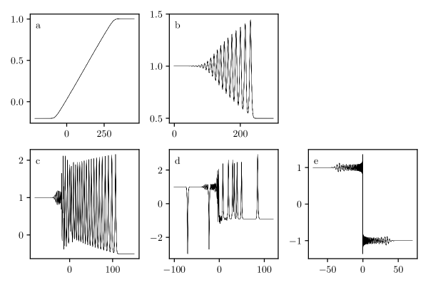
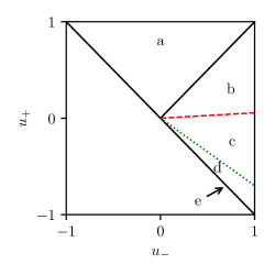
a	$|u_{-}|<u_{+}$	convex RW
b	$\mu\,u_{-}<u_{+}<u_{-}$	convex DSW
c	$\sigma_{3}(\xi)\,u_{-}<u_{+}<\mu\,u_{-}$	DSW implosion
d	$-u_{-}<u_{+}<\sigma_{3}(\xi)\,u_{-}$	incoherent waves
e	$u_{+}=-u_{-}<0$	dispersive Lax shock

Figure 1: Classification of the BBM dispersive Riemann problem (1.4), (1.7) in the $u_{+}+u_{-}\geq 0$ half plane (triangle) when $\xi\gg 1$. Corresponding representative numerical simulations for $\xi=10$ in each case are shown. The table is a description of the partitioning and wave patterns. $\mu=e^{-3/2}/4\approx 0.056$, $\sigma_{3}(\xi)$ is generally unknown but empirically $\sigma_{3}(10)\approx-0.70$.

Large transition width $\xi\gg 1$, Figure 1

When $u_{+}>\max(\mu u_{-},-u_{-})$ where $\mu=e^{-3/2}/4$, convex RWs (region $a$) and DSWs (region $b$) are generated, qualitatively similar to those generated by KdV (1.3) evolution. In Sec. 6.2, we use the DSW fitting approach to make quantitative predictions for the DSW’s properties (edge velocities, harmonic edge wavenumber, soliton edge amplitude, and DSW structure near the harmonic edge). We also identify the loss of convexity at the harmonic edge (where a zero linear dispersion point is attained) as the progenitor for nonclassical wave patterns when $u_{+}$ is below the line $\mu u_{-}$.

For initial data sufficiently close to the line $u_{+}=\mu u_{-}$ (region $c$), DSW implosion occurs. A weakly nonlinear, two-phase modulation theory using coupled nonlinear Schrödinger equations is developed in Sec. 6.3, the two wave envelopes associated with modulations of short and long waves, respectively. We find that there is a spatial redistribution of energy from the long waves in a partial DSW on the right to a short wave wavepacket on the left. The partial DSW is typically accompanied by some number of depression envelope solitary waves. Very similar DSW implosion dynamics are also observed in the small transition width regime $\xi\ll 1$ (see region $f$ in Fig. 2).

There exists a stationary, discontinuous compressive shock solution of the BBM equation when $u_{+}=-u_{-}<0$ (region $e$). In Sec. 4.1, we show that smoothed step initial data for this case exhibits the usual nonlinear self-steepening but is also accompanied by the continued production of shorter and shorter waves during evolution. In a neighborhood of $x=0$, an oscillatory overshoot appears that quickly saturates to a constant magnitude. An approximate self-similar solution in the form $u(x,t)=g(xt)$ is obtained that describes these oscillations as $t\to\infty$. This feature is reminiscent of Gibbs’ phenomenon in the theory of Fourier series and linear dispersive partial differential equations with discontinuous initial data [7]. We refer to this wave pattern as a dispersive Lax shock. However, if the initial data is perturbed asymmetrically so that $-u_{-}<u_{+}<\sigma_{3}(\xi)u_{-}$ (region $d$), then the evolution exhibits a large number of solitary waves and highly oscillatory wavepackets that do not exhibit a discernible, coherent pattern. We refer to this as the incoherent solitary wave regime and describe it in Subsection 6.4. The dispersive Lax shock and the incoherent solitary wave patterns also occur for small transition width $\xi\ll 1$ (see regions $h$ and $g$ in Fig. 2).

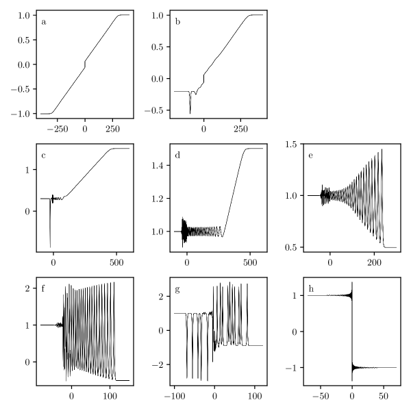
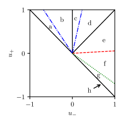
a	$0<\!-u_{-}\!\leq\!u_{+}\!<\!-\sigma_{1}(\xi)\,u_{-}$	expansion shock
b	$0<-\sigma_{1}(\xi)\,u_{-}<u_{+}$	exp shock $\!\!+\!\!$ solis
c	$0<\sigma_{2}(\xi)\,u_{-}<u_{+}$	RW $\!\!+\!\!$ solis $\!\!+\!\!$ lin waves
d	$u_{-}<u_{+}<\sigma_{2}(\xi)\,u_{-}$	RW $\!\!+\!\!$ lin waves
e	$\mu\,u_{-}<u_{+}<u_{-}$	DSW $\!\!+\!\!$ lin waves
f	$\sigma_{3}(\xi)\,u_{-}<u_{+}<\mu\,u_{-}$	DSW implosion
g	$-u_{-}<u_{+}<\sigma_{3}(\xi)\,u_{-}$	incoherent waves
h	$u_{+}=-u_{-}<0$	dispersive Lax shock

Figure 2: Classification of the BBM dispersive Riemann problem (1.4), (1.7) when $\xi\ll 1$. The triangle is a partitioning of the boundary data in the $u_{+}+u_{-}\geq 0$ half plane. Corresponding representative numerical simulations for $\xi=0.1$ in each case are shown. The table is a description of the partitioning and wave patterns. $\mu=e^{-3/2}/4\approx 0.056$, $\sigma_{2}(\xi)=1+\sqrt{6\beta}\xi^{1/2}+\sqrt{27\beta/8}\xi^{5/2}+\cdots$, $\beta\approx 9.5$, $\sigma_{3}(\xi)$ is generally unknown but empirically $\sigma_{3}(0.1)\approx-0.70$. $\sigma_{1}(\xi)$ is generally unknown but empirically $\sigma_{1}(0.1)\approx 0.68$.

Small transition width $\xi\ll 1$, Figure 2

Generally, the features observed for large transition width in Fig. 1 persist into the small transition width regime shown in Fig. 2 but with modification. Rarefaction waves are accompanied by a decaying expansion shock in regions $a$ and $b$, depression solitary waves propagating to the left in regions $b$ and $c$, and small amplitude linear waves propagating to the left in regions $c$ and $d$.

From the ideal expansion shock solution for symmetric data ($u_{-}=-u_{+}<0$) (reviewed in Sec. 4.3) into region $a$ for asymmetric data, a short-time analysis of the solution reveals an asymmetry that favors the generation of a depression wave for $x<0$ (Sec. 5.2). When the threshold $u_{+}=-\sigma_{1}(\xi)u_{-}$ is exceeded, the asymmetry produces a solitary wave that is shed from the expansion shock. Greater asymmetry generates the shedding of more depression solitary waves until $u_{+}\geq 0$ and an expansion shock is no longer generated. Nevertheless, solitary wave shedding persists until $u_{+}=\sigma_{2}(\xi)u_{-}$. Solitary Wave shedding thresholds $\sigma_{1}(\xi)$ and $\sigma_{2}(\xi)$ are analyzed in Sec. 5.3.

When $u_{-}\geq 0$ (regions $c$–$e$), the small transition width gives rise to the generation of small amplitude wavepackets that accompany the RW or DSW. In the absence of solitary wave shedding, we can conveniently partition the initial smoothed step in the Fourier domain to prescribe initial data for the linearized BBM equation. In Sec. 3, long-time asymptotic analysis of the solution integral yields a precise prediction for three distinct wavepacket regimes corresponding to one-phase, two-phase, and Airy modulations. The analysis of DSW implosion (regions $c$ and $f$ in Figs. 1 and 2, respectively) can be viewed as a weakly nonlinear generalization of the linear wavepacket analysis.

The dynamics of DSW implosion (region $f$), incoherent waves (region $g$), and the dispersive Lax shock (region $h$) are qualitatively similar to the respective regions in the large transition width case identified in Fig. 1.

A general conclusion from our analysis, in both the large and small transition width regimes, is that the loss of linear dispersion convexity underlies the generation of nonclassical wave patterns.

3 Linear wavetrains and Airy modulation near the zero dispersion point

In this section, we investigate the asymptotic structure of the approximately linear wavetrains generated in BBM dispersive Riemann problems with smoothed step initial data (1.7) in the parameter domain $(u_{-},u_{+},\xi)$ defined by: $0<u_{-}$, $\mu<u_{+}/u_{-}<\sigma_{2}(\xi)$, where $\mu={\rm e}^{-3/2}/4$ and $\sigma_{2}(\xi)$ is defined later in equation (5.31); see regions $d$ and $e$ in Fig. 2. The significance of $\sigma_{1,2}$ will be clarified later. Depending on the relative values of $u_{-}$ and $u_{+}$, the initial step generates either a RW ($u_{-}<u_{+}$ ) or a DSW ($u_{-}>u_{+}$). In both cases, an approximately linear wavetrain develops on the background $u=u_{-}$ behind the RW or DSW and occupies an expanding region $x\in[x_{0}^{-}(t),x_{0}^{+}(t)]$, where the right boundary $x_{0}^{+}$ coincides with the trailing edge of the RW or DSW and $x_{0}^{-}$ will be determined. In this section, we use linear theory to analyze the corresponding wavetrains, hence we refer to them as “linear wavetrains”, with an understanding that this is an approximation.

3.1 Linear wavetrains in the BBM Riemann problem

We start by linearizing the BBM equation (1.4) about a constant background $\overline{u}>0$, $u(x,t)=\overline{u}+\varphi(x,t)$, $|\varphi|\ll\overline{u}$, and obtain

$$\varphi_{t}+\overline{u}\varphi_{x}-\varphi_{xxt}=0.$$ (3.1)

For $\varphi\propto\exp[i(kx-\omega t)]$, we obtain the BBM linear dispersion relation:

$$\omega=\omega_{0}(k,\overline{u})=\overline{u}\frac{k}{1+k^{2}}.$$ (3.2)

Then the group velocity is given by the first derivative of $\omega_{0}$

$$\partial_{k}\omega_{0}=\overline{u}\frac{1-k^{2}}{(1+k^{2})^{2}},$$ (3.3)

and the dispersion sign is defined by the sign of the second derivative

$$\mathrm{sgn}\left(\partial_{kk}\omega_{0}\right)=\mathrm{sgn}\left(\overline{u}\frac{2k(k^{2}-3)}{(1+k^{2})^{3}}\right).$$ (3.4)

The dispersion relation is nonconvex and the dispersion sign is zero for $k=0$, $k=\sqrt{3}$ or $\overline{u}=0$. We stress that it is the non-convexity of the linear dispersion relation (3.2) that gives rise to crucial differences between the BBM and KdV dispersive Riemann problems. The KdV linear dispersion relation is strictly convex for $k>0$.

The group velocity (3.3) has a minimum when $k=\sqrt{3}$,

$$\partial_{k}\omega_{0}\geq s_{\min}(\overline{u})=-\frac{\overline{u}}{8},$$ (3.5)

and a maximum at $k=0$,

$$\partial_{k}\omega_{0}\leq s_{\max}(\overline{u})=\overline{u}.$$ (3.6)

Consequently, a BBM linear wavetrain that develops from a localized initial disturbance considered in isolation on the constant background $\overline{u}$ is confined to the region $x\in[s_{\min}t,s_{\max}t]$ in the asymptotic regime $t\gg 1$, although some rapidly decaying oscillations are possible outside this region. We now place this in the context of the dispersive Riemann problem where the linear wavetrain is generated on the background $\overline{u}=u_{-}$ as part of the nonlinear-dispersive regularization of smoothed step initial data. We consider two cases $u_{-}<u_{+}$ and $u_{-}>u_{+}$ separately, distinguishing between a linear wave trailing a RW or a DSW (see Fig. 2(d,e)).

(i) First, consider the case $u_{-}<u_{+}$ that leads to a RW. As we shall see later in Sec. 4.2, the trailing edge of the RW is located at $x=u_{-}t=s_{\max}(u_{-})t$. Provided $u_{+}/u_{-}<\sigma_{2}(\xi)$, no solitary wave propagates in the region $x<s_{\max}t$ (cf. Sec. 4.2). Thus the two kinds of structures generated in this class of BBM dispersive Riemann problems—the linear wavetrain for $x\in[s_{\min}(u_{-})t,s_{\max}(u_{-})t]$, and the RW for $x\in[u_{-}t,u_{+}t]$—do not overlap and can be described separately, except in the vicinity of the point $x=u_{-}t$ where the two solutions could be matched. A linear wavetrain can also be generated for $u_{+}/u_{-}\geq\sigma_{2}$ but we do not consider this case because one or more solitary waves may accompany the wavetrain, complicating its analysis.

(ii) For the case $u_{-}>u_{+}$, which leads to a DSW, we show in Sec. 6 that the trailing edge of the DSW is located at $x=s_{-}t<s_{\max}(u_{-})t$ so that the trailing linear wavetrain is necessarily attached to the DSW. For $u_{+}/u_{-}>\mu$, we have $s_{\min}(u_{-})<s_{-}$ and our main concern here will be the description of the linear wavetrain located outside the vicinity of the DSW trailing edge point $x=s_{-}t$, where the two modulated wavetrains could be matched.

Summarizing, we assume that for dispersive Riemann problems with $\mu<u_{+}/u_{-}<\sigma_{2}(\xi)$, the generation and propagation of a small-amplitude wavetrain is governed by the linearized BBM equation (3.1) with $\overline{u}=u_{-}$, and its dynamics are fully decoupled from the nonlinear DSW or RW dynamics. In other words, we suppose that the initial profile’s Fourier spectrum can be partitioned into two essentially distinct components. The short-wave (large wavenumber) component of the spectrum is assumed to evolve according to the linear wave equation (3.1). The long-wave (small wavenumber) component of the spectrum is assumed to evolve according to the nonlinear BBM equation (1.4). Consequently, the linear wave evolution is superposed with the nonlinear evolution. We justify our partition of the initial Fourier spectrum by comparison of our linear analysis with numerical simulations. Since the Fourier transform of the initial condition (1.7) is given by the formula,

$${\cal F}[u_{0}(x)]=\int_{\mathbb{R}}u_{0}(x)e^{-ikx}dx=\frac{u_{+}-u_{-}}{2i}\frac{\pi\xi}{\sinh(\pi\xi k/2)}+\pi(u_{+}+u_{-})\delta(k),$$ (3.7)

the partitioning assumption implies that the Fourier transform of the linear wave $\varphi(x,t)$ at $t=0$ is approximated by

$$\hat{\varphi}_{0}(k)={\cal F}[\varphi(x,0)]\sim\displaystyle\frac{u_{+}-u_{-}}{2i}\frac{\pi\xi}{\sinh(\pi\xi k/2)},\quad\forall k\in\mathbb{R}.$$ (3.8)

The initial condition (3.8) simplifies for a step ($\xi\to 0$) to $\hat{\varphi}_{0}(k)=(u_{+}-u_{-})/ik$, $k>k_{0}$. Note that $|\hat{\varphi}_{0}(k)|$ is a rapidly decaying function of $\xi$, and so no linear wavetrain is expected to be generated for $\xi\gg 1$. This agrees with Fig. 1, which shows the evolution for the dispersive Riemann problem with $\xi=10$.

The solution of (3.1), is given by

$$\varphi(x,t)=\frac{1}{2\pi}\int_{\mathbb{R}}\hat{\varphi}_{0}(k)e^{-i\chi(k)t}dk,\quad\chi(k)=\omega_{0}(k,u_{-})-k\frac{x}{t},$$ (3.9)

For notational convenience, we suppress the dependence of $\chi$ on $\frac{x}{t}$.

3.2 Stationary phase analysis

Consider the asymptotic regime $t\to\infty$ with $x/t$ fixed. We can evaluate the integral (3.9) using the stationary phase method, cf. for instance [51]. Fast oscillations average out in the integral, and the main contribution comes from the neighborhood of the stationary points $k_{n}$ defined as solutions of $\chi^{\prime}(k)=0$, namely

$$\partial_{k}\omega_{0}=u_{-}\frac{1-k_{n}^{2}}{(1+k_{n}^{2})^{2}}=x/t.$$ (3.10)

A first approximation of $\varphi(x,t)$ is obtained by substituting the Taylor expansions:

$$\hat{\varphi}_{0}(k)=\hat{\varphi}_{0}(k_{n})+{\cal O}\left[k-k_{n}\right],\quad\chi(k)=\chi(k_{n})+\frac{\partial_{k}^{2}\chi(k_{n})}{2}(k-k_{n})^{2}+{\cal O}\left[(k-k_{n})^{3}\right].$$ (3.11)

Equation (3.10) implies that $k_{n}$ depends on $s\equiv x/t$. The computation of (3.9) thus reduces to the integration of a Gaussian, and the corresponding solution $\varphi$ only depends on the number of stationary points and their respective positions in $k$-space:

$$\varphi(x,t)\sim\frac{1}{2\pi}\sum_{n}\hat{\varphi}_{0}(k_{n})e^{-i\chi(k_{n})t}\int_{\mathbb{R}}e^{-i\,\partial_{kk}\omega_{0}(k_{n},u_{-})(k-k_{n})^{2}t/2}dk.$$ (3.12)

Real solutions of (3.10) come in pairs $(-k_{n},k_{n})$ and, since $\hat{\varphi}_{0}(-k)=\hat{\varphi}^{*}_{0}(k)$ and $\omega_{0}(-k,u_{-})=-\omega_{0}(k,u_{-})$, the sum in (3.12) simplifies to [51]:

$$\varphi(x,t)\sim\frac{1}{\pi}\sum_{k_{n}>0}\Re\left[\hat{\varphi}_{0}(k_{n})e^{-i\chi(k_{n})t}\int_{\mathbb{R}}e^{-i\,\partial_{kk}\omega_{0}(k_{n},u_{-})k^{2}t/2}dk\right].$$ (3.13)

The stationary phase equation (3.10) divides space-time into two regions.

(a) In the region $s_{\rm max}>s=x/t>0$, denoted hereafter as Region I, (3.10) has only one positive solution

$$0<k_{1}=\sqrt{\frac{-u_{-}-2s+\sqrt{u_{-}(u_{-}+8s)}}{2s}}\leq\sqrt{3},\quad s\in(0,s_{\rm max}),$$ (3.14)

so the series (3.13) has just one term. This is comparable to what we would obtain with a convex linear dispersion relation, and we refer to this region as the convex linear regime. In fact, for $k\ll 1$, we obtain the linear dispersion relation $\omega_{0}(k,\overline{u})\sim\overline{u}(k-k^{3})$, which is the linear dispersion relation for the KdV equation.

(b) In the region $s_{\rm min}<s=x/t<0$, denoted hereafter as Region II, (3.10) has $k_{1}(s)$ and an additional positive solution

$$k_{2}(s)=\sqrt{\frac{-u_{-}-2s-\sqrt{u_{-}(u_{-}+8s)}}{2s}}\geq\sqrt{3},\quad s\in\left(s_{\rm min},0\right),$$ (3.15)

so that the series (3.13) has two terms. The coexistence of two waves with wavenumbers $k_{1}$ and $k_{2}$ at the same position $x$ within Region II is a direct consequence of the nonconvexity of the dispersion relation (3.2). The modulation of the linear wave in this region dramatically differs from a convex-dispersion, KdV-type linear modulation. In Sec. 6.3 below, we show that the coexistence of two dominant wavenumbers also persists in the nonlinear regime, leading to the phenomenon of DSW implosion. The upper panel of Fig. 3 displays the comparison between the wavenumber of the waves obtained numerically from the full partial differential equation (PDE) simulation, shown in the lower panel, and the graph of $x$ given by (3.10) as a function of $k=k_{n}$ for a fixed value of $t,$ with $k_{n}$, $n=1,2$ given by the formulas (3.14), (3.15). The two regions I and II are treated separately using the stationary phase approximation (3.13). A third region, denoted III in Fig. 3 and defined hereafter as $x\lesssim s_{\rm min}t$, is resolved with an expansion near $x=s_{\min}t.$

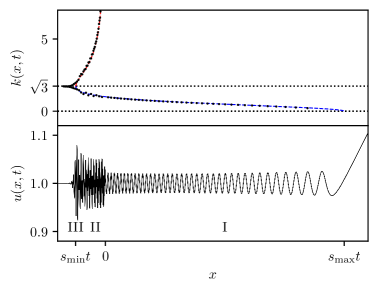
Figure 3: The lower panel displays the variation of the dispersive Riemann problem’s numerical solution with $\xi=0.1$, $u_{-}=1$ and $u_{+}=1.5$ at $t=500$. The solution is well-approximated by a one-phase linear wave in region I and a two-phase linear wave in region II. The variation of the waves’ wavenumber extracted from the numerical solution is represented by black disks in the upper panel; the procedure to extract wavenumbers in region II is detailed in Appendix A.2. The blue (red) dashed line corresponds to the variation of the analytical solutions $k_{1}(x,t)$ ($k_{2}(x,t)$).

(Region I)  In the convex linear regime of Region I, the stationary phase approximation yields

$$\varphi(x,t)\sim\sqrt{\frac{2}{\pi}}\Re\left[\frac{\hat{\varphi}_{0}(k_{1})}{\sqrt{|\partial_{kk}\omega_{0}(k_{1},u_{-})|t}}e^{i[k_{1}x-\omega_{0}(k_{1},u_{-})t]-i\,\mathrm{sgn}[\partial_{kk}\omega_{0}(k_{1},u_{-})]\pi/4}\right].$$ (3.16)

Since $\arg[\hat{\varphi}_{0}(k_{1})]=-\pi/2$ and $\partial_{kk}\omega_{0}(k_{1},u_{-})<0$, we have

$$\varphi(x,t)\sim\varphi_{\rm I}(x,t)=|\hat{\varphi}_{0}(k_{1})|\sqrt{\frac{2}{\pi|\partial_{kk}\omega_{0}(k_{1},u_{-})|t}}\cos\left[k_{1}x-\omega_{0}(k_{1},u_{-})t-\frac{\pi}{4}\right].$$ (3.17)

This solution is not valid close to the so-called caustic trajectory $x=u_{-}t=s_{\rm max}t,$ where the two dominant wavenumbers $k_{1}$ and $-k_{1}$ coalesce at $k_{1}=0$, (cf. for instance [9]) and $\partial_{kk}\omega_{0}(k_{1},u_{-})=0$. At this edge of Region I, one needs to consider the next order in the expansion of $\chi(k)$ in the Taylor expansion (3.11). Besides, as pointed out earlier, a RW or a DSW develops close to the point $x/t=u_{-}$ or $x/t=s_{-}<u_{-}$ (respectively), and the linear wave has to be asymptotically matched with the hydrodynamic state. Such a higher order derivation, which can be achieved by following the matched asymptotics procedure developed for the KdV equation [22, 33], is not important for us here because we have a well-defined initial value problem (3.1), (3.8). The comparison between the approximate solution (3.17) and the numerical solution of the dispersive Riemann problem in region I is displayed in Fig. 4.

(Region II)  In Region II, for which $x\in[s_{\min}t,0]$, the modulated wave corresponding to the large wavenumber branch $k_{2}$ coexists with the wave from the lower wavenumber branch $k_{1}$, leading to a modulated beating pattern. The stationary phase approximation then yields the superposition

$$\begin{split}\varphi(x,t)&\sim\sqrt{\frac{2}{\pi}}\Re\left[\frac{\hat{\varphi}_{0}(k_{1})}{\sqrt{-\partial_{kk}\omega_{0}(k_{1},u_{-})t}}e^{i[k_{1}x-\omega_{0}(k_{1},u_{-})t]+i\pi/4}+\frac{\hat{\varphi}_{0}(k_{2})}{\sqrt{\partial_{kk}\omega_{0}(k_{2},u_{-})t}}e^{i[k_{2}x-\omega_{0}(k_{2},u_{-})t]-i\pi/4}\right],\\ &=\sqrt{\frac{2}{\pi}}\Bigg{(}\frac{|\hat{\varphi}_{0}(k_{1})|}{\sqrt{|\partial_{kk}\omega_{0}(k_{1},u_{-})|t}}\cos\left[k_{1}x-\omega_{0}(k_{1},u_{-})t-\frac{\pi}{4}\right]\\ &\qquad\qquad+\frac{|\hat{\varphi}_{0}(k_{2})|}{\sqrt{|\partial_{kk}\omega_{0}(k_{2},u_{-})|t}}\cos\left[k_{2}x-\omega_{0}(k_{2},u_{-})t-\frac{3\pi}{4}\right]\Bigg{)}.\end{split}$$ (3.18)

(Region III)  The approximation (3.18) fails to describe the oscillations of the linear wave for $x/t$ close to $s_{\min}$, corresponding to the zero dispersion point where the two branches coalesce: $k_{1}=k_{2}=\sqrt{3}$, $\partial_{kk}\omega_{0}(\sqrt{3},u_{-})=0$. In this region, the expansion (3.11) is insufficient. We shall denote the union of this special region $s\sim s_{\rm min}$ and $s<s_{\rm min}$ as $s\lesssim s_{\rm min}$ and call it Region III. In order to describe the oscillations in this region, we expand $\chi(k)$ close to the inflection point $k=\sqrt{3}$

$$\chi(k)=\omega_{0}(\sqrt{3},u_{-})-\sqrt{3}\,x/t-(x/t-s_{\rm min})(k-\sqrt{3})+\frac{\partial_{kkk}\omega_{0}(\sqrt{3},u_{-})}{6}t(k-\sqrt{3})^{3}+{\cal O}[(k-\sqrt{3})^{4}].$$ (3.19)

Substituting this expansion into eq. (3.9), we obtain

$$\varphi(x,t)\sim\frac{1}{\pi}\Re\left[\hat{\varphi}_{0}(\sqrt{3})e^{i[\sqrt{3}x-\omega_{0}(\sqrt{3},u_{-})t]}\int_{\mathbb{R}}e^{i(x-s_{\rm min}t)(k-\sqrt{3})-i\,\partial_{kkk}\omega_{0}(\sqrt{3},u_{-})(k-\sqrt{3})^{3}t/6}dk\right].$$ (3.20)

With the change of variable $k-\sqrt{3}\to-\alpha\kappa$ with $\alpha=(2/\partial_{kkk}\omega_{0}(\sqrt{3},u_{-})t)^{1/3}$, the approximation becomes

$$\varphi(x,t)=2\alpha|\hat{\varphi}_{0}(\sqrt{3})|{\rm Ai}[-\alpha(x-s_{\min}t)]\cos\left[\sqrt{3}\left(x-\frac{u_{-}}{4}t\right)-\frac{\pi}{2}\right],\quad\alpha=\left(\frac{32}{3u_{-}t}\right)^{1/3}\ll 1,$$ (3.21)

where ${\rm Ai}(y)$ is the Airy function defined by [2]

$${\rm Ai}(y)=\frac{1}{2\pi}\int_{\mathbb{R}}e^{i(\kappa y+\kappa^{3}/3)}d\kappa\in\mathbb{R}.$$ (3.22)

The solution (3.21) represents a harmonic cosine wave modulated by the Airy function. Note that the Airy approximation (3.21) is also valid for $x/t<s_{\min}$, where the Airy modulation describes an exponential decay of the wave’s amplitude: ${\rm Ai}(y)\sim y^{-1/4}\exp(-\tfrac{2}{3}y^{3/2})$ as $y\to+\infty$, which in our case translates to $(x-s_{\min}t)\to-\infty$.

3.3 Uniform Airy approximation

Using the technique originally developed in [8], we derive a uniform approximation that is valid in the union of regions II and III whose limiting behavior is given by (3.21) when $x\lesssim s_{\rm min}t$ and (3.18) when $x\gg s_{\rm min}t$. We summarize here the derivation detailed in [9]. First, we suppose that the solution in region II accords with the ansatz

$$\varphi(x,t)=\frac{1}{\pi}\Re\left[\int_{\mathbb{R}}(\phi_{0}+\kappa\phi_{1})e^{i(A-\kappa\zeta+\kappa^{3}/3)}d\kappa\right],$$ (3.23)

where $\phi_{0}\in\mathbb{C}$, $\phi_{1}\in\mathbb{C}$, $A\in\mathbb{R}$ and $\zeta\in\mathbb{R}$ are functions of $(x,t)$ that are to be determined. By selecting the exponential’s phase $\psi=A-\kappa\zeta+\kappa^{3}/3$, we will ensure that it has the same stationary points as $\chi(k)$ for $x$ close to $s_{\rm min}t$. Note that, although only the leading order term $\hat{\varphi}_{0}(k_{n})$ in the Taylor expansion of $\hat{\varphi}_{0}(k)$ near $k=k_{n}$ in the approximations leading to (3.13) and (3.20) was used, incorporating the first order term $\hat{\varphi}_{0}^{\prime}(k_{n})(k-k_{n})$ in the analysis is essential for constructing a uniform approximation. We first determine the functions $\phi_{0}$, $\phi_{1}$, $A$ and $\zeta$ by evaluating the integral (3.23) using the stationary phase method. For simplicity, we consider the computation for $\zeta>0$; the computation is similar in the case $\zeta<0$, cf. [9]. The phase $\psi$ has two stationary points:

$$\kappa=\pm\sqrt{\zeta}.$$ (3.24)

Close to the stationary points $\pm\sqrt{\zeta}$, the phase is given by

$$\psi=A\mp\frac{2}{3}\zeta^{3/2}\pm\sqrt{\zeta}(\kappa\mp\sqrt{\zeta})^{2}+{\cal O}[(\kappa\mp\sqrt{\zeta})^{3}]$$ (3.25)

Substituting the Taylor expansion of $\psi$ into (3.23), we obtain (cf. previous stationary phase computations)

$$\varphi(x,t)\sim\frac{1}{\sqrt{\pi}}\Re\left[\frac{\phi_{0}+\sqrt{\zeta}\phi_{1}}{\zeta^{1/4}}e^{i(A-2\zeta^{3/2}/3)+i\pi/4}+\frac{\phi_{0}-\sqrt{\zeta}\phi_{1}}{\zeta^{1/4}}e^{i(A+2\zeta^{3/2}/3)-i\pi/4}\right].$$ (3.26)

Since the solution (3.23) should be asymptotically valid in all of region II, we impose that (3.26) identify with (3.18) for $x\gg s_{\rm min}t$. The identification imposes

$$\begin{split}&A=\frac{1}{2}\Big{[}(k_{1}+k_{2})x-(\omega_{0}(k_{1},u_{-})+\omega_{0}(k_{2},u_{-}))t\Big{]},\quad\zeta^{3/2}=-\frac{3}{4}\Big{[}(k_{1}-k_{2})x-(\omega_{0}(k_{1},u_{-})-\omega_{0}(k_{2},u_{-}))t\Big{]},\\ &\phi_{0}=\frac{\zeta^{1/4}\hat{\varphi}_{0}(k_{1})}{\sqrt{-2\partial_{kk}\omega_{0}(k_{1},u_{-})t}}+\frac{\zeta^{1/4}\hat{\varphi}_{0}(k_{2})}{\sqrt{2\partial_{kk}\omega_{0}(k_{2},u_{-})t}},\quad\phi_{1}=\frac{\zeta^{-1/4}\hat{\varphi}_{0}(k_{1})}{\sqrt{-2\partial_{kk}\omega_{0}(k_{1},u_{-})t}}-\frac{\zeta^{-1/4}\hat{\varphi}_{0}(k_{2})}{\sqrt{2\partial_{kk}\omega_{0}(k_{2},u_{-})t}}.\end{split}$$ (3.27)

Then, direct integration of (3.23) yields:

$$\varphi(x,t)=\varphi_{\rm uni}(x,t)=2\Re\left[e^{iA}(\phi_{0}{\rm Ai}(-\zeta)-i\phi_{1}{\rm Ai}^{\prime}(-\zeta))\right],$$ (3.28)

where ${\rm Ai}(y)$ is given by (3.22) and ${\rm Ai}^{\prime}(y)\equiv d{\rm Ai}/dy$. By construction, (3.28) is asymptotic to (3.18) when $x\gg s_{\rm min}t$, i.e. $\zeta\gg 1$. Additionally, $\phi_{0}\sim 2\alpha\hat{\varphi}_{0}(\sqrt{3})$, $\phi_{1}\sim-\alpha^{2}\hat{\varphi}_{0}(\sqrt{3})/\sqrt{3}$, and $\zeta=-\alpha(x-s_{\rm min}t)$, such that the uniform approximation (3.28) asymptotically matches with the Airy approximation (3.21) when $x\sim s_{\rm min}t$ (recall that $\alpha\ll 1$ in the long time regime). Note that the uniform approximation (3.28) is also valid in the region $x<s_{\rm min}t$, or equivalently $\zeta<0$, where the analytical expressions (3.14) and (3.15) are complex.

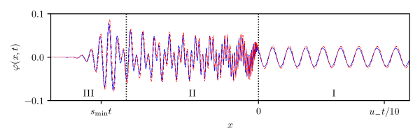
Figure 4: Comparison between the asymptotic stationary phase solution (3.29) (red dash-dotted line) with the solution of the dispersive Riemann problem obtained numerically at $t=500$ for $(\xi,u_{-},u_{+})=(0.1,1,1.5)$ (blue solid line).

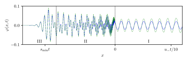
Figure 5: Comparison between the solutions $\varphi=u(x,t)-u_{-}$ of the dispersive Riemann problems $(\xi,u_{-},u_{+})=(0.1,1,1.5)$ (blue solid line) and $(\xi,u_{-},u_{+})=(0.1,1,0.5)$ (green dashed line) at $t=500$. Note that, according to (3.8), the linear wave depends on the sign of $u_{+}-u_{-}$ and the green line represents the field $-\varphi(x,t)$ with $u_{-}>u_{+}$ in order to be compared to the solution $\varphi(x,t)$ with $u_{-}<u_{+}$.

To summarize, the linear wave generated by the dispersive Riemann problem is approximated by the piecewise-defined function

$$\varphi(x,t)\sim\begin{cases}\varphi_{\rm uni}(x,t),&x\leq 0,\\ \varphi_{\rm I}(x,t),&0<x,\end{cases},\quad t\gg 1,\quad\frac{x}{t}=\mathcal{O}(1),$$ (3.29)

where $\varphi_{\rm I}$ and $\varphi_{\rm uni}$ are defined in (3.17) and (3.28), respectively. This stationary phase approximation compares well with the numerical solution, as displayed in Fig. 4.

An important consequence of the approximate initial data (3.8) for $\varphi$ is that the linear wave solution $\varphi(x,t)$ is valid for both polarities of the initial jump $u_{-}<u_{+}$ and $u_{-}>u_{+}$, i.e., for either the generation of waves accompanying a RW or the generation of waves accompanying a DSW, respectively. Moreover, the linear waves accompanying a RW, $\varphi_{\rm RW}(x,t)$, with jump $u_{+}-u_{-}>0$ are related to the linear waves accompanying a DSW with the same jump magnitude $u_{-}-u_{+}>0$ by a minus sign: $\varphi_{\rm DSW}(x,t)=-\varphi_{\rm RW}(x,t)$. Figure 5 displays the numerical solutions for two different initial conditions $u_{-}<u_{+}$ and $u_{-}>u_{+}$ with a common difference magnitude $|u_{+}-u_{-}|$. Although the two numerical solutions are comparable, the discrepancy between them increases with increasing $x$; the discrepancy is larger in Region I. In fact, the small amplitude assumption at the core of linear theory is not well-fulfilled since, initially, $|\varphi(x,0)|={\cal O}(|u_{-}-u_{+}|)$. It is, therefore, remarkable that linear theory still predicts the evolution of the fast oscillations with excellent accuracy, even if the small amplitude assumption is initially violated. The discrepancy in Fig. 5 is due to different matching conditions for the linear wave with the leftmost, trailing edge of the RW or DSW. This asymptotic matching has been investigated for the KdV equation in [33, 22].

Finally, we note that the asymptotic behavior (3.21) near the zero dispersion point is general and can be obtained for other wave equations exhibiting a non-convex linear dispersion relation. For example, it was obtained (with appropriate modifications due to a different form of the dispersion relation) in [49] for linear wavepackets in the Gardner-Ostrovsky equation.

4 Shocks and rarefactions

In this section, we consider shock wave and rarefaction wave solutions of the underlying conservation law $u_{t}+uu_{x}=0$ and their role in the structure of solutions of the dispersive Riemann problem for the BBM equation. Stationary shocks play a significant part in this description (regions $e$ and $h$ in Figs. 1 and 2, respectively), since they are also weak solutions of the BBM equation. Of particular interest are stationary shocks that are either compressive (satisfying the Lax entropy condition) or expansive (violating the Lax condition). Stationary compressive shocks are a major feature of our analysis of dispersive Riemann problem solutions for data $(u_{-},u_{+})$ in regions d, e of Fig. 1 and g, h of Fig. 2 while stationary expansion shocks are important in regions a and b of Fig. 2. Without loss of generality, we suppose that $|u_{+}|=1$; the solution with $|u_{+}|=b\neq 1$ is given by the change of variable $(x,t,u)\to(x,t/b,bu)$.

4.1 Stationary Lax shocks

We first consider the solution when $u_{-}=-u_{+}=1$. Both the Hopf $u_{t}+uu_{x}=0$ and the BBM equation (1.4) admit the stationary, discontinuous, weak solution

$$u(x,t)=\begin{cases}1&x\leq 0\\ -1&x>0\end{cases},$$ (4.1)

or stationary Lax shock. The shock wave is compressive in the sense that the Hopf characteristics (with speed $u_{\pm}=\mp 1$) on each side of the shock located at $x=0$ propagate into the shock [32]. Although this BBM solution has been acknowledged elsewhere, e.g. [15], it has remained mostly a curiosity.

We investigate the dynamics when (4.1) is smoothed at $t=0$ according to (1.7) with $u_{\pm}=\mp 1$. The numerical solution $u(x,t)$ is displayed in Fig. 6 at different times.

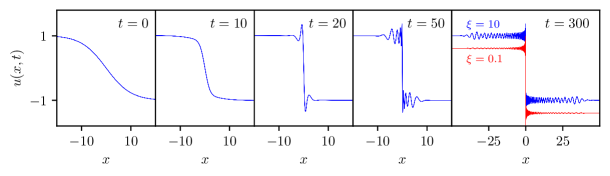
Figure 6: Numerical solution of the dispersive Riemann problem with $u_{-}=-u_{+}=1$ and $\xi=10$ at times shown. The last plot displays the numerical solution starting with a smoothed, steep step where $\xi=0.1$; a different color and an offset have been added to distinguish the variations of the two solutions.

Evolution initially leads to the usual nonlinear self steepening ($t=10$) due to broad initial data ($\xi=10$). This long wave, Hopf equation-like evolution, is soon accompanied by oscillations ($t=20$) when the solution is steep enough and the BBM dispersive term $u_{xxt}$ is important. Dispersive regularization of shock formation typically results in a DSW (cf. Sec. 6), with an expanding collection of oscillations. The long-time dynamics of a generic DSW consists of finite amplitude waves that are bounded in wavenumber [16]. But here, oscillations of increasing, apparently unbounded wavenumber develop as time increases, concentrating near the origin. The last panel of Fig. 6 ($t=300$) shows that the large $t$ behavior for both broad and narrow initial smoothed step profiles approach approximately the same structure, suggesting the existence of some self-similar asymptotic configuration. We remark that a previous numerical study of BBM has depicted similar behavior for broad, periodic initial data [21], associating it with discontinuity formation.

To further investigate these dynamics, we introduce the short space $\rho=x/\epsilon$ and long time $T=\epsilon t$ scaling where $0<\epsilon\ll 1$ is a small parameter representing the characteristic length scale of the oscillations in a neighborhood of the origin. With this scaling, the BBM equation (1.4) becomes

$$\epsilon u_{T}+\frac{1}{\epsilon}uu_{\rho}=\frac{1}{\epsilon}u_{\rho\rho T}.$$ (4.2)

Expanding $u$ in $\epsilon$ as $u=U_{0}(\rho,T)+\epsilon U_{1}(\rho,T)+\cdots$, we obtain the leading order equation

$$U_{0}\partial_{\rho}U_{0}=\partial_{\rho\rho T}U_{0}.$$ (4.3)

This equation can be integrated once in $\rho$, yielding a nonlinear Klein-Gordon equation

$$\frac{1}{2}U_{0}^{2}-\alpha=\partial_{\rho T}U_{0}.$$ (4.4)

In general, $\alpha$ is an arbitrary function of $T$. Motivated by the numerical observations in Fig. 6, we seek a self-similar solution that must be independent of the small but otherwise arbitrary parameter $\epsilon$, thus can only depend on $\rho T=xt$:

$$U_{0}(\rho,T)=g(\eta),\quad\eta=\rho T=xt.$$ (4.5)

In order for $g$ to satisfy a well-defined ordinary differential equation (ODE)

$$\left(\eta g^{\prime}\right)^{\prime}+\alpha-\frac{1}{2}g^{2}=0,\quad^{\prime}\equiv\frac{d}{d\eta},$$ (4.6)

we require $\alpha\in\mathbb{R}$ to be constant. The boundary condition $u(x,t)\to-1$ as $x\to\infty$ implies $g(\eta)\to-1$ as $\eta\to\infty$. Linearizing equation (4.6) about the boundary condition $g(\eta)=-1+h(\eta)$ where $|h|\ll 1$, we obtain the equation

$$\left(\eta h^{\prime}\right)^{\prime}+\alpha-\frac{1}{2}+h=0.$$ (4.7)

If the integration constant is set to $\alpha=1/2$, then $h(\eta)=0$ is a stable fixed point of the homogeneous equation (4.7) with the general, Bessel-type solution $h(\eta)=C_{1}J_{0}(2\sqrt{\eta})+C_{2}Y_{0}(2\sqrt{\eta})$, for some $C_{1},C_{2}\in\mathbb{R}$. Consequently, the large $\eta$ asymptotics of the Bessel solution demonstrate that the sought solution to eq. (4.6) with $\alpha=1/2$ exhibits algebraic, oscillatory decay to the requisite boundary condition

$$g(\eta)\sim-1+\frac{C}{\eta^{1/4}}\cos\left(2\sqrt{\eta}-\phi\right),\quad\eta\to\infty,$$ (4.8)

for some constants $C$ and $\phi$.

Since the symmetric, smoothed step initial data considered here is an odd function of $x$, we seek a solution to (4.6) that is an odd function of its argument so that $g(0)=0$. Evaluating eq. (4.6) at $\eta=0$ also determines $g^{\prime}(0)=-1/2$. The initial conditions

$$g(0)=0,\quad g^{\prime}(0)=-\frac{1}{2},$$ (4.9)

uniquely determine the solution of eq. (4.6) with $\alpha=1/2$ that decays to $-1$ according to (4.8). We compute the numerical solution to this initial value problem and display the result in Fig. 7. Motivated by the linearized equation (4.7), we also plot in 7 the function $-1+J_{0}(2\sqrt{\eta}-0.7)$, which provides a good empirical fit to $g(\eta)$ when $2\sqrt{\eta}\gtrsim 8$. By the asymptotics of the Bessel function $J_{0}$, we can infer from Fig. 7 that $C\approx\pi^{-1/2}$ and $\phi\approx\pi/4+0.7$ in eq. (4.8).

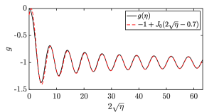
Figure 7: Self-similar dispersive Lax shock profile (solid, black) and a Bessel function approximation (dashed, red).

In Fig. 8, the numerical solution of the dispersive Riemann problem for both narrow and broad initial data approaches the self-similar solution $g(xt)$ (with an odd extension) for large $t$. The narrow case in 8(a) leads to the development of oscillations with wavelengths that are shorter than the self-similar profile whereas the broad case in 8(b) exhibits longer wavelength oscillations than $g(\eta)$. In both cases, there is no indication of discontinuity formation in finite time.

Since the odd-extended self-similar solution $g(\eta)\to\pm 1$ as $\eta\to\mp\infty$, we observe that it converges to the stationary Lax shock (4.1) as $t\to\infty$ for each fixed $x$

$$\lim_{t\to\infty}g(xt)=\begin{cases}1,&x<0\\ 0,&x=0\\ -1,&x>0\end{cases},$$ (4.10)

although the convergence is not uniform in $x$. The self-similar, oscillatory profile $g(xt)$ describes how the stationary Lax shock develops as $t\to\infty$. Based on these observations, we call the profile $g(xt)$ a dispersive Lax shock. This asymptotic solution represents a completely new type of dispersive shock structure.

The simulations in Figs. 6 and 8 exhibit behavior reminiscent of Gibbs phenomenon in the theory of Fourier series. Perhaps a more apt comparison is to initial value problems for linear dispersive PDE in which the data is discontinuous [7]. For a broad class of constant coefficient, linear dispersive PDE, the convergence of the solution as $t\to 0^{+}$ for initial data with a discontinuity is not uniform. Moreover, it exhibits Gibbs phenomenon whereby the solution has an overshoot that, in proportionality to the jump, converges to the Wilbraham-Gibbs constant

$$\mathfrak{g}\equiv\frac{1}{\pi}\int_{0}^{\pi}\frac{\sin{z}}{z}dz-\frac{1}{2}\approx 0.08949.$$ (4.11)

In contrast, the dispersive Lax shock $g(xt)$ converges to the discontinuity (4.10) as $t\to\infty$. While the oscillations for $\eta$ sufficiently far from $0$ are linear and Bessel-like, the compression of these oscillations is an inherently nonlinear process. Narrower oscillations appear as the initial smoothed step profile steepens and approaches a jump discontinuity. In contrast to the aforementioned linear initial value problems, we observe an oscillatory overshoot that can be numerically estimated from the self-similar profile $g(xt)$ to be, in proportion to the jump height,

$$\max_{\eta\in\mathbb{R}}\frac{g(\eta)-1}{2}\approx 0.18342,$$ (4.12)

a bit more than twice the Wilbraham-Gibbs constant $\mathfrak{g}$.

Numerical simulations are limited by the discretization and method utilized. The structure and self-similar scaling of $g(xt)$ will, for large enough $t$, exceed the resolution of any fixed discretization scheme. Our analysis of this dispersive Riemann problem provides a means to interpret solutions in the vicinity of dispersive Lax shocks.

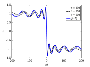
(a) $\xi=0.1$

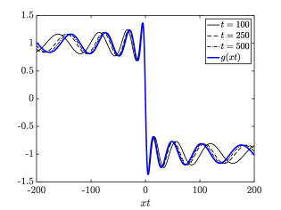
(b) $\xi=10$

Figure 8: Numerical solution for $u(x,t)$ at different times (solid, dashed, dash-dotted) tending toward the self-similar solution $g(xt)$ (thick, blue) for narrow (a) and broad (b) symmetric smoothed step initial data $u_{\pm}=\mp 1$.

We show in Sec. 6.3 that the solution of the dispersive Riemann problem for slightly asymmetric boundary conditions $0<u_{-}+u_{+}\ll u_{-}$ is drastically different from the symmetric case investigated here. In particular, we will show that solitary waves are shedded in an incoherent fashion on top of a compressive shock structure.

4.2 Rarefaction waves

From now on, we consider the case $u_{+}=1$. In Fig. 9, we show numerical solutions of (1.4), (1.7) with $u_{-}<1$. Dispersive effects are negligible for smoothed step initial data ($\xi\gg 1$), and the asymptotic solution of the dispersive Riemann problem is a smoothed modification of the RW solution

$$u(x,t)=u_{\rm RW}(x,t)=\begin{cases}u_{-},&x<u_{-}t,\\ x/t,&u_{-}t\leq x<t,\\ 1,&t\leq x,\end{cases}$$ (4.13)

of the dispersionless equation $u_{t}+uu_{x}=0.$ Fig. 9(b) displays good agreement between the form (4.13) and the smooth RW numerical solution of equation (1.4).

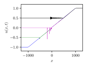
(a) Narrow smoothed step initial data $\xi=0.1$. Numerical solutions at an earlier time are displayed in Figs. 11 and 12.

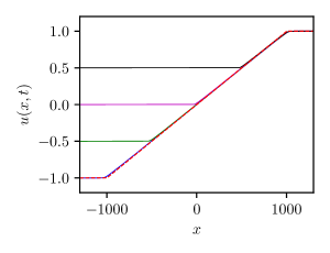
(b) Broad smoothed step initial data $\xi=10$. The dashed red line corresponds to the analytical RW solution (4.13) with $u_{-}=1$.

Figure 9: Solutions of the dispersive Riemann problem (1.4),(1.7) with $u_{-}<1$ at $t=1000$. Solid lines correspond to numerical solutions with $u_{-}\in\{-1,-0.5,0,0.5\}$.

Dispersive effects are more significant for narrow smoothed step initial data ($\xi\ll 1$), as demonstrated dramatically in Fig. 9(a) and later on in Figs. 10 and 12. In the case of symmetric initial conditions $u_{-}=-1$, the RW develops with an expansion shock that is described in Sec. 4.3 below. The evolution of asymmetric smoothed step initial data (having $-1<u_{-}<1$) displays richer structure (cf. Fig. 9(a)). The interplay between long and short waves in the linear regime (clearly visible in Fig. 9(a) with $u_{-}=1/2)$ is analysed in Sec. 3, and the emergence of a train of solitary waves is investigated in Sec. 5. We show in Sec. 5.2 that the development of expansion shock and solitary wavetrain structures for $\xi\to 0$ is linked to the atypical early time evolution of the dispersive Riemann problem.

4.3 Expansion shocks

Consider the initial condition (1.7) with $u_{-}=-1$, i.e.

$$u_{0}(x)=\tanh\left(\frac{x}{\xi}\right),$$ (4.14)

with $\xi\ll 1$. In [15], an asymptotic solution is derived in detail, using $\xi$ as a small parameter, with long-time scaling $T=\xi t$. Here, we outline the description in [15].

The inner structure of the solution, near $x=0,$ is described using the same short space scaling $\chi=x/\xi$ as that utilized for the description of the dispersive Lax shock in Sec. 4.1. However, the small parameter $\xi$ in this case is fixed by the choice of initial data (1.7). These scalings introduced into the BBM equation (1.4) lead to

$$\xi u_{T}+\frac{1}{\xi}uu_{\chi}=\frac{1}{\xi}u_{\chi\chi T}.$$ (4.15)

Expanding $u$ in $\xi$: $u=U_{0}(\chi,T)+\xi U_{1}(\chi,T)+{\cal O}(\xi^{2})$, we obtain the leading order equation

$$U_{0}\partial_{\chi}U_{0}=\partial_{\chi\chi T}U_{0}.$$ (4.16)

In addition to the self-similar solution to this equation that we obtained for the dispersive Lax shock, here we obtain a separated solution describing the expansion shock. Equation (4.16) with initial condition $U_{0}(\chi,0)=\tanh\left(\chi\right)$ corresponding to (4.14), admits the separated solution

$$U_{0}(\chi,t)=\frac{1}{1+T/2}\tanh{\chi}.$$ (4.17)

Thus the inner solution of the dispersive Riemann problem (1.4), (4.14) for $\xi\ll 1$ is given by

$$u(x,t)=\frac{1}{1+\xi t/2}\tanh\left(\frac{x}{\xi}\right)+{\cal O}(\xi),\quad|x|=\mathcal{O}(\xi),\quad t=\mathcal{O}\left(\frac{1}{\xi}\right).$$ (4.18)

The outer structure of the solution is described using the long space scaling $X=\xi x,$ leading to

$$\xi u_{T}+\xi uu_{X}=\xi^{3}u_{XXT}.$$ (4.19)

Looking for $u$ in the form  $\tilde{U}_{0}(X,T)+\xi\tilde{U}_{1}(X,T)+{\cal O}(\xi^{2})$, we obtain the Hopf equation at leading order

$$\partial_{T}\tilde{U}_{0}+\tilde{U}_{0}\partial_{X}\tilde{U}_{0}=0.$$ (4.20)

The general solution of this equation is $\tilde{U}_{0}=f(X-\tilde{U}_{0}T)$. The matching of $\tilde{U}_{0}$ with the inner solution (4.17), $\lim_{|X|\to 0}\tilde{U}_{0}(X,T)=\lim_{|\chi|\to\infty}U_{0}(\chi,T)$, yields

$$\tilde{U}_{0}(X,T)=\frac{{\rm sgn}(X)+X/2}{1+T/2}.$$ (4.21)

This formula is continuously matched with the far-field conditions: $\lim_{x\to\pm\infty}u=\pm 1$, leading to the outer solution,

$$u(x,t)=\begin{cases}\dfrac{{\rm sgn}(x)+\xi x/2}{1+\xi t/2},&|x|<t,\\[6.0pt] {\rm sgn}(x),&|x|>t,\end{cases}+{\cal O}(\xi),\quad|x|=\mathcal{O}\left(\frac{1}{\xi}\right),\quad t=\mathcal{O}\left(\frac{1}{\xi}\right).$$ (4.22)

Combining the descriptions (4.18) and (4.22), we obtain the uniformly valid asymptotic solution of (1.4), (4.14) for $\xi\ll 1$

$$u(x,t)=u_{\rm exp}(x,t)=\frac{1}{1+\xi t/2}\big{[}\tanh(x/\xi)-{\rm sgn}(x)\big{]}+\begin{cases}\dfrac{{\rm sgn}(x)+\xi x/2}{1+\xi t/2},&|x|<t.\\[10.0pt] {\rm sgn}(x),&|x|>t.\end{cases}$$ (4.23)

As remarked in [15], the accuracy of the asymptotic solution (4.23) is excellent, cf. Fig. 10. Note that the expansion shock structure converges to the rarefaction solution (4.13) as $t\to\infty$.

We also observe in Fig. 10 that the expansion shock persists for slightly asymmetric boundary conditions with $-1<u_{-}<0$, and $u_{+}=1,$ see for instance the solution for $u_{-}=-0.7$. The outer solution for such conditions is a slight modification of (4.22)

$$u(x,t)=\begin{cases}u_{-},&x<u_{-}t+2\frac{u_{-}+1}{\xi},\\[6.0pt] \dfrac{{\rm sgn}(x)+\xi x/2}{1+\xi t/2},&u_{-}t+2\frac{u_{-}+1}{\xi}\leq x<t,\\[6.0pt] 1,&t\leq x,\end{cases}\quad|x|=\mathcal{O}\left(\frac{1}{\xi}\right),\quad t=\mathcal{O}\left(\frac{1}{\xi}\right),$$ (4.24)

which is continuous at $x=u_{-}t$. Thus the truncated solution reads:

$$u(x,t)=u_{\rm aexp}(x,t)=\frac{1}{1+\xi t/2}\big{[}\tanh(x/\xi)-{\rm sgn}(x)\big{]}+\begin{cases}u_{-},&x<u_{-}t+2\frac{u_{-}+1}{\xi},\\[6.0pt] \dfrac{{\rm sgn}(x)+\xi x/2}{1+\xi t/2},&u_{-}t+2\frac{u_{-}+1}{\xi}\leq x<t,\\[6.0pt] 1,&t\leq x.\end{cases}$$ (4.25)

Fig. 10 shows that the asymmetric solution is in very good agreement with the numerical solution for values of $u_{-}$ sufficiently close to $-1$. The absolute error between the analytical and the numerical solutions is represented in Fig. 11 for $u_{-}=-0.7$. The largest error at $t=1/\xi=10$ is approximately $\xi$ and decreases with time as expected. In the next section, we analyze the generation of solitary waves on top of the expansion shock for larger values of $u_{-}$.

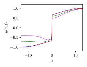
(a) $t=1/\xi=10$

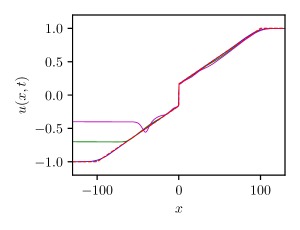
(b) $t=10/\xi=100$

Figure 10: Solutions of the dispersive Riemann problem (1.4), (1.7) with $u_{-}<0$ and $\xi=0.1$. The solid lines correspond to numerical solutions with $u_{-}\in\{-1,-0.7,-0.4\}$. The red dashed line corresponds to the expansion shock solution $u_{\rm exp}$ (4.23); the truncated solution (4.25) is given by $u_{\rm exp}$ for $x\geq u_{-}t$ and $u_{-}$ for $x<u_{-}t$.

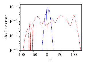
Figure 11: Pointwise error between the truncated expansion shock (4.25) and numerical solution $\xi=0.1,\;u_{-}=-0.7$ at $t=10$ (blue solid line) and $t=100$ (red dashed line).

5 Solitary wave shedding

In this section, we study the generation of solitary waves observed in numerical solutions. Throughout this section, we keep $u_{+}=1$ and consider $-1<u_{-}<1,$ with $\xi\ll 1$ (regions a, b, c, and d in Fig. 2). Numerical results, described in Sec. 5.1, exhibit a train of solitary waves for a range of values of $u_{-}$. However, for $x>0,$ the solutions have either a rarefaction wave accompanied by a region I linear wave (described in Sec. 3), or a portion of the expansion shock solution (described in Sec. 4.3). There are no solitary waves generated in the region $x>0$. We can therefore restrict attention to $x<0$.

In Sec. 5.2, we explain the appearance of solitary waves by analyzing the early time behavior of the solutions. In Sec. 5.3, we use the energy equality satisfied by smooth solutions, to establish the values of $u_{-}$ for which a solitary wave is generated from those for which the solution has no solitary wave.

5.1 Numerical Solutions

We start with a qualitative description of the numerical solutions shown in Fig. 12 for various values of $u_{-}<1$ and fixed $\xi=0.1$. As expected from Sec. 3, a linear wave develops to the left of the RW when $u_{-}>0$. Moreover, solitary waves of negative polarization are additionally generated for sufficiently small values $u_{-}<u_{-}^{(2)}\approx 0.23$ of $u_{-}$ as depicted in Fig. 12(a). This threshold first appears at the line $L_{2}$, $u_{+}=\sigma_{2}(\xi)u_{-}$, of Fig. 2. The solitary wave solution of the BBM equation (1.4) is given by [40]

$$u(x,t)=\overline{u}+u_{\rm sol}(x,t;c,\overline{u})=\overline{u}+3(c-\overline{u}){\rm sech}^{2}\left(\sqrt{1-\frac{\overline{u}}{c}}\,\frac{x-ct}{2}\right),$$ (5.1)

where $c$ is the wave speed and $\overline{u}$ is the background value. The wave amplitude is $a=3(c-\overline{u})$ yielding the speed-amplitude relation

$$c=c(a,\overline{u})=\overline{u}+a/3.$$ (5.2)

Note that the solitary wave solution exists only for $c\in\mathbb{R}\backslash[\min(\overline{u},0),\max(\overline{u},0)]$. The example $\overline{u}=u_{-}=0.2$ in Fig. 12(a) shows that the emitted solitary wave is locally well described by the analytical profile (5.1).

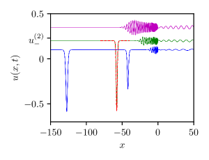
(a) Positive left boundary conditions: $u_{-}\in\{0.1,0.2,0.35\}$. The dashed red line represents the solitary wave solution (5.1) with the parameter: $\overline{u}=u_{-}=0.2$ and $c=-5.9\times 10^{-2}$.

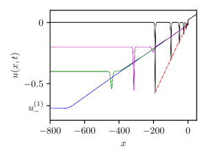
(b) Negative left boundary conditions: $u_{-}\in\{-0.7,-0.4,-0.2,0\}$. The dash-dotted red line represents the amplitude variation given by the relation $c(a,u_{-}=0)=x/t$.

Figure 12: Numerical solutions of the dispersive Riemann problem, with $\xi=0.1$ at $t=1000$.

If $\overline{u}=u_{-}=0$, the linear dispersion relation (3.2) is $\omega_{0}(k,\overline{u})=0,$ and only a train of solitary waves is generated for $x<0$ as in Fig. 12(b). Similarly, when $u_{-}<0$, although a linear wave can propagate on a strictly negative background, its group velocity satisfies $\partial_{k}\omega_{0}>u_{-}$ so that no linear waves remain in the region $x<u_{-}t$ for $t\gg 1$. The solitary wavetrain then propagates from the tail of the truncated expansion shock solution (4.25), as depicted in Fig. 12(b). No solitary wave emission is observed when $u_{-}<u_{-}^{(1)}\approx-0.68$. The variation of the amplitude of the leftmost solitary wave amplitude with $u_{-}\in[u_{-}^{(1)},u_{-}^{(2)}]$ is depicted in Fig. 13.

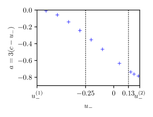
Figure 13: Amplitude of the leftmost solitary wave for $u_{-}\in[u_{-}^{(1)},u_{-}^{(2)}]$ with $u_{-}^{(1)}=-0.68$ and $u_{-}^{(2)}=0.23$. The dashed vertical lines delimit the region $u_{-}\in[-0.25,0.13]$ where multiple solitary waves are generated.

We empirically observe that when $u_{-}\in(u^{\rm(a)},0]$ and multiple solitary waves are emitted, the amplitude $a(x,t)$ of the solitary wavetrain asymptotically satisfies $c(a,u_{-})=x/t$ where $c$ is the speed-amplitude relation (5.2). A detailed study of the solitary wavetrain using, for example, Whitham modulation theory [51], is left as a subject for future work.

5.2 Early time evolution

The unusual generation of linear waves and solitary waves can be qualitatively explained by investigating the early time dynamics of the dispersive Riemann problem. We consider in this section the small-time expansion of the solution

$$u(x,t)=u_{0}(x)+tu_{1}(x)+{\cal O}(t^{2}),$$ (5.3)

where $u_{0}(x)$ is given by (1.7) with $u_{+}=1$. Substituting (5.3) into (1.4), we obtain at the zeroth order in $t$

$$u_{1}^{\prime\prime}-u_{1}=u_{0}u_{0}^{\prime},$$ (5.4)

where ${}^{\prime}\equiv d/dx$. The small parameter condition $tu_{1}(x)\ll u_{0}(x)$ yields the boundary conditions: $\lim_{x\to\pm\infty}u_{1}(x)=0$. Let $G(x)$ be the Green’s function satisfying,

$$G^{\prime\prime}(x)-G(x)=\delta(x),$$ (5.5)

given by

$$G(x)=-\exp(-|x|)/2.$$ (5.6)

The solution of (5.4) is then

$$u_{1}(x)=\int\limits_{-\infty}^{+\infty}G(x-y)\frac{d}{dy}\left(\frac{u_{0}^{2}(y)}{2}\right)dy=\frac{1}{4}\int\limits_{-\infty}^{+\infty}{\rm sgn}(x-y)e^{-|x-y|}u_{0}^{2}(y)dy.$$ (5.7)

Note that $u_{1}(x)$ (and higher order terms) can be directly obtained from the integro-differential form of the BBM equation (1.8) by iteration, which is part of the contraction mapping argument used to prove local existence of solutions to the BBM initial value problem [4]. The correction $u_{1}(x)$ is bounded by

$$|u_{1}(x)|\leq\frac{1}{4}\int\limits_{-\infty}^{+\infty}e^{-|y-x|}\left|\frac{d}{dy}\left(u_{0}^{2}(y)\right)\right|dy<\frac{1-u_{-}}{2\xi},$$ (5.8)

an estimate that decreases with increasing $\xi,$ so that $u_{1}$ is negligible for large $\xi.$

On the other hand, in the ideal case $\xi\to 0,$ the initial condition is the step given by (1.6), and (5.7) simplifies to

$$u_{1}(x)=\frac{u_{-}^{2}-1}{4}\,e^{-|x|}<0,$$ (5.9)

leading to a decrease in $u(x,t)$ for sufficiently small $t>0$. This introduces a dip in the graph of $u(x,t)$ for $x<0.$ The small amplitude assumption $tu_{1}(x)\ll 1-u_{-}$ (recall that $1-u_{-}$ represents the initial smoothed step height) then reduces to $t\ll 1/(1+u_{-})$. Figure 14(a) shows good agreement between the approximate solution (5.3) with (5.9) and the corresponding numerical solution of the dispersive Riemann problem when $\xi=0.1.$ While the initial smoothed step is rarefying in the region $x>0$, a dip develops immediately in the region $x<0$. As a result, the initial smoothed step transition persists, contrasting with numerical solutions for $\xi=10$ (Fig. 14(b)) that more closely resemble the classical RW, with no dip developing.

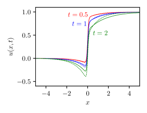
(a) $\xi=0.1$: The dashed lines correspond to the approximate solution $u_{0}(x)+tu_{1}(x),$ with $u_{1}$ given by (5.9).

(b) $\xi=10$: No dip develops for a slowly varying initial condition.

Figure 14: Numerical solution (solid curves) of the smoothed step dispersive Riemann problem (1.4), (1.7) at different times.

Figure 15 displays different evolution scenarios of smoothed step initial data for $\xi=0.1$ depending on the value of $u_{-}$. If $u_{-}^{\rm(2)}<u_{-}$ (case a) the smoothed step emits a linear wavepacket. Additionally, solitary waves are generated if $0<u_{-}\leq u_{-}^{\rm(2)}$ as depicted in case b. If $u_{-}=0$ (case c), the smoothed step decays into a solitary wavetrain. The solitary wavetrain behavior can be recognized by monitoring the region close to the expansion shock in the long time regime, as in the contour plot of Fig. 16. The early time evolution changes for $u_{-}^{(1)}\leq u_{-}<0$ (case d) where the smoothed step also generates solitary waves but fewer than the $u_{-}=0$ case. For $u_{-}<0$, the initial smoothed step persists in the form of the approximate truncated expansion shock solution (4.25). In all of these cases, the solution $u(x,t)$ converges to the rarefaction wave solution (4.13) as $t\to\infty,$ for each fixed $x.$

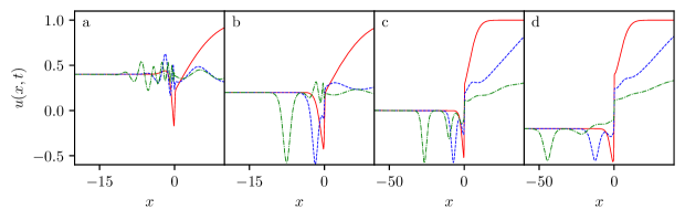
Figure 15: Initial evolution of the smoothed step dispersive Riemann problem (1.4), (1.7) for $\xi=0.1$. The solution is plotted for three different times: $t=10$ (red solid line), $t=50$ (blue dashed line) and $t=150$ (green dash-dotted line). a) $u_{-}=0.4$, b) $u_{-}=0.2$, c) $u_{-}=0$, d) $u_{-}=-0.2$.

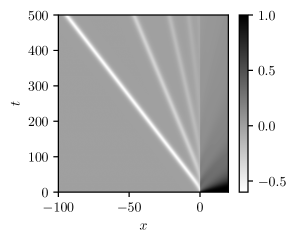
Figure 16: Spatio-temporal evolution of the solitary wavetrain generated for $\xi=0.1$ and $u_{-}=0$. The colors are inverted: light (dark) colors correspond to small (large) values of the solution $u(x,t)$. The smoothed step or dip in the vicinity of $x=0$ is radiating negative solitary waves with different speeds in the region $x<0$.

5.3 The threshold for generation of a negative solitary wave

In this subsection, we derive the conditions for and properties of the emitted solitary wave in the simplest case where only one solitary wave is shedded, cf. Fig. 13. We also determine the threshold $u_{-}=u_{-}^{\rm(2)}>0$ for which solitary waves are generated adjacent to the RW for any value of $\xi\ll 1$. Up to now the value of the parameter $u_{-}^{\rm(2)}$ has been obtained numerically for the value $\xi=0.1$.

The derivation of the solitary wave’s speed (or equivalently amplitude using the speed-amplitude relation (5.2)) is achieved using the mass conservation law (the BBM equation itself)

$$u_{t}+\left(\tfrac{1}{2}u^{2}-u_{xt}\right)_{x}=0.$$ (5.10)

and an additional energy conservation law satisfied by smooth solutions [40]

$$\left(\tfrac{1}{2}u^{2}+\tfrac{1}{2}u_{x}^{2}\right)_{t}+\left(\tfrac{1}{3}u^{3}-uu_{xt}\right)_{x}=0.$$ (5.11)

Integration of (5.10) and (5.11) between the limits $x=-L$ and $x=+L$ yields

$$\frac{dN}{dt}+\left[\tfrac{1}{2}u^{2}-u_{xt}\right]_{-L}^{+L}=0,$$ (5.12)

$$N(t)=\int\limits_{-L}^{+L}u\,dx,$$ (5.13)

$$\frac{dE}{dt}+\left[\tfrac{1}{3}u^{3}-uu_{xt}\right]_{-L}^{+L}=0,$$ (5.14)

$$E(t)=\int\limits_{-L}^{+L}\frac{u^{2}+u_{x}^{2}}{2}dx.$$ (5.15)

Because of the term $u_{x}^{2}$, the initial energy $E(t=0)$, obtained by substituting the initial smoothed step (1.7) in (5.15), strongly depends on the transition width $\xi,$ which plays a crucial role in the appearance of negative solitary waves, as was demonstrated numerically in Fig. 9.

Motivated by observations in Sec. 5.1, we suppose that when $u_{-}$ is very close to $u_{-}^{\rm(2)}$, the solution $u(x,t)$ can be approximated for large $t$ by

$$u(x,t)=u_{\rm RW}(x-b,t)+u_{\rm sol}(x,t;c,u_{-})+\varphi(x,t),\qquad c<s_{\rm min}=-u_{-}/8<0,\qquad t\gg 1,$$ (5.16)

where $b$ and $c$ remain to be determined. Expressions for $u_{\rm RW}$ and $u_{\rm sol}$ are given in (4.13) and (5.1), respectively, and $\varphi(x,t)$ is a correction term. We suppose here that the RW is not centered and denote $b$ the value of the shift. The incorporation of the RW shift is crucial for the precise determination of the threshold for solitary wave emission and the accompanying solitary wave’s speed $c$. Figure 17(a) shows the necessity of incorporating a vertical shift $-b/t$ of the centered RW solution $u_{\rm RW}(x,t)$ in order to achieve good agreement with the numerical simulation. We also hypothesize that the dominant contribution to the correction $\varphi(x,t)$ is a linear wavetrain, analogous to that studied in Sec. 3. Note that the solitary wave and the linear wavetrain correction propagate on the background $\overline{u}=u_{-}$, fixed by the boundary condition. Thus, the condition $c<s_{\rm min}$ ensures that the solitary wave is negative and that it is well-separated from the RW and the linear wavetrain for $t\gg 1$. This assumption is consistent with numerical computations. We now show that the formula (5.16) represents a solution of the dispersive Riemann problem (1.4),(1.7) for a certain value of the solitary wave speed $c$ depending on $\xi\ll 1$ and $u_{-}$.

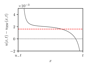
(a) RW solution $(\xi,u_{-})=(0.1,0.18)$. The dashed red line corresponds to the shift $u_{\rm RW}(x-b,t)-u_{\rm RW}(x,t)=-b/t$; $b\approx-1.61$ is given by the resolution of (5.28).

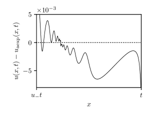
(b) Asymmetric expansion wave solution $(\xi,u_{-})=(0.1,-0.3)$.

Figure 17: Absolute error of the hydrodynamic state at $t=1000$ when a solitary wave is generated.

In a first approximation, we suppose that the correction $\varphi(x,t)$ has a negligible mass and energy contribution:

$$u(x,t)\sim u_{\rm RW}(x-b,t)+u_{\rm sol}(x,t;c,u_{-}),\qquad t\gg 1.$$ (5.17)

We evaluate the mass $N(t)$ and the energy $E(t)$ in two different ways: i) by direct substitution of (5.17) in (5.13) and (5.15) and ii) by solving (5.12) and  (5.14) with the initial condition (1.7) and the boundary conditions $\lim_{x\to\pm\infty}u(x,t)=u_{\pm}$, $\lim_{x\to\pm\infty}u_{xt}(x,t)=0$. Equating the two expressions for $N(t)$ and $E(t)$ then yields an approximation to the solitary wave speed $c$ and the RW shift $b$.

(i)  The direct substitution of the ansatz (5.17) into (5.13) yields

$$N=N_{\rm RW}+N_{\rm sol},\quad N_{\rm RW}=\int\limits_{-L}^{+L}u_{\rm RW}dx,\quad N_{\rm sol}=\int\limits_{-L}^{+L}(u_{\rm sol}-u_{-})dx,$$ (5.18)

and the direct substitution of the ansatz (5.17) into (5.15) yields

$$E=E_{\rm RW}+E_{\rm sol},\quad E_{\rm RW}=\int\limits_{-L}^{+L}\frac{u_{\rm RW}^{2}+(\partial_{x}u_{\rm RW})^{2}}{2}dx,\quad E_{\rm sol}=\int\limits_{-L}^{+L}\frac{u_{\rm sol}^{2}+2u_{-}u_{\rm sol}+(\partial_{x}u_{\rm sol})^{2}}{2}dx.$$ (5.19)

We choose $L$ and $t$ such that: $L\gg t\gg 1$. The contribution of the RW to the energy then simplifies to

$$N_{\rm RW}=\frac{u_{-}^{2}-1}{2}t+(u_{-}+1)L+(u_{-}-1)b,$$ (5.20)

$$E_{\rm RW}=\frac{u_{-}^{3}-1}{3}t+\frac{1-u_{-}}{2t}+\frac{u_{-}^{2}+1}{2}L+\frac{u_{-}^{2}-1}{2}b\sim\frac{u_{-}^{3}-1}{3}t+\frac{u_{-}^{2}+1}{2}L+\frac{u_{-}^{2}-1}{2}b.$$ (5.21)

Since $L\gg 1$ and $u_{\rm sol}(x,t;c)$ decays exponentially to $0$ when $|x|\to\infty$, we can allow $L\to\infty$ in the integral for $N_{\rm sol}$ and $E_{\rm sol}$

$$N_{\rm sol}(c,u_{-}) \sim\int\limits_{-\infty}^{+\infty}(u_{\rm sol}-u_{-})dx=12\sqrt{1-\frac{u_{-}}{c}}c$$ (5.22)

$$E_{\rm sol}(c,u_{-}) \sim\int\limits_{-\infty}^{+\infty}\frac{u_{\rm sol}^{2}+2u_{-}u_{\rm sol}+(\partial_{x}u_{\rm sol})^{2}}{2}dx=\frac{12}{5}\sqrt{1-\frac{u_{-}}{c}}\left(\frac{6c^{2}}{u_{-}^{2}}-\frac{2c}{u_{-}}+1\right)u_{-}^{2}.$$ (5.23)

(ii)  Now we consider the conservation laws (5.12) and (5.14). Since $L\gg t$, the RW and the solitary wave have not reached the positions $x=\pm L$ at the time $t$ and the solution $u(x,t)$ decays rapidly to $u_{\pm}$ for $|x|\sim L$. In particular, we have $u\sim u_{\pm}$ and $|u_{xt}|\ll u_{\pm}^{2}$ at $x=\pm L$. Thus the conservation laws read

$$\frac{dN}{dt}\sim\frac{u_{-}^{2}-1}{2},\quad\text{which yields}\quad N\sim\frac{u_{-}^{2}-1}{2}t+N(0),\quad N(0)=\int\limits_{-L}^{+L}u_{0}\,dx,$$ (5.24)

$$\frac{dE}{dt}\sim\frac{u_{-}^{3}-1}{3},\quad\text{which yields}\quad E\sim\frac{u_{-}^{3}-1}{3}t+E(0),\quad E(0)=\int\limits_{-L}^{+L}\frac{u_{0}^{2}+(\partial_{x}u_{0})^{2}}{2}dx,$$ (5.25)

where $u_{0}$ is the smoothed step initial data (1.7). We calculate

$$N(0)=(u_{-}+1)L,\quad E(0)=\frac{(u_{-}^{2}+1)L}{2}+\frac{(u_{-}+1)^{2}\tanh(L/\xi)\left[3-3\xi^{2}-\tanh^{2}(L/\xi)\right]}{12\xi}.$$ (5.26)

Since $L\gg\xi$, the initial energy $E(0)$ simplifies to

$$E(0)\sim\frac{(u_{-}^{2}+1)L}{2}+(u_{-}-1)^{2}\left(\frac{1}{6\xi}-\frac{\xi}{4}\right).$$ (5.27)

Equating (5.18) and (5.24), and  (5.19) and (5.25) yields

$$N_{\rm sol}(c,u_{-})+(u_{-}-1)b=0,\quad E_{\rm sol}(c,u_{-})+\frac{u_{-}^{2}-1}{2}b=(u_{-}-1)^{2}\left(\frac{1}{6\xi}-\frac{\xi}{4}\right),$$ (5.28)

which combine into a single equation for the solitary wave speed $c$

$$E_{\rm sol}(c,u_{-})-\frac{u_{-}+1}{2}N_{\rm sol}(c,u_{-})=(u_{-}-1)^{2}\left(\frac{1}{6\xi}-\frac{\xi}{4}\right).$$ (5.29)

A solitary wave emerges to the left of the linear wavetrain if (5.29) has a solution $c<-u_{-}/8$. This is the case if and only if $u_{-}<u_{-}^{\rm(2)}$ where $u_{-}^{\rm(2)}$ solves the equation:

$$E_{\rm sol}\left(-\frac{u_{-}^{\rm(2)}}{8},u_{-}^{\rm(2)}\right)-\frac{u_{-}^{\rm(2)}+1}{2}N_{\rm sol}\left(-\frac{u_{-}^{\rm(2)}}{8},u_{-}^{\rm(2)}\right)=\left(u_{-}^{\rm(2)}-1\right)^{2}\left(\frac{1}{6\xi}-\frac{\xi}{4}\right).$$ (5.30)

Since $\xi\ll 1$, we have the approximation

$$u_{-}\leq u_{-}^{\rm(2)}=1/\sigma_{2}(\xi),\quad\sigma_{2}(\xi)=1+\frac{9}{2}\sqrt{\frac{21}{5}\xi}+\frac{27}{4}\xi+{\cal O}(\xi^{3/2}).$$ (5.31)

The critical value $u_{-}^{\rm(2)}=1/\sigma_{2}(\xi)$ constitutes the threshold for the emission of one solitary wave in the dispersive Riemann problem. This formula compares quantitatively with the threshold obtained numerically for different values of $\xi$ as displayed in Fig. 18(a).

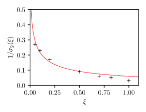
(a) Variation of the threshold for the generation of a solitary wave when $u_{-}<1/\sigma_{2}(\xi)$. The red solid line corresponds to (5.31) and the crosses to the thresholds determined numerically.

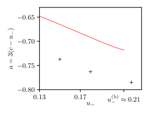
(b) Amplitude of the shedded solitary wave for $\xi=0.1$. The red solid line corresponds to the solution of (5.29).

Figure 18: Solitary wave shedding with $u_{-}>0$ in the regime $\xi\ll 1$

Suppose now $\sigma_{2}(\xi)u_{-}\leq 1$. Solving (5.29) for $c(u_{-})$, we obtain the solitary wave’s amplitude $a(u_{-})=3[c(u_{-})-u_{-}]$ in function of $u_{-}$. Figure 18(b) displays the variation of $c(u_{-})$ when $\xi=0.1$, which compares reasonably well with the amplitude of the emitted solitary wave obtained numerically.

Discrepancy between the analytical results and the numerics in Fig. 18 is due to neglecting the linear corrective term $\varphi$ in the ansatz (5.16). Because it separates from the RW and solitary wave, the contribution of the linear wave to the mass and the energy are

$$N_{\varphi}=\int_{s_{\rm min}t}^{u_{-}t}(u-u_{-})dx,\quad E_{\varphi}=\int_{s_{\rm min}t}^{u_{-}t}\frac{u^{2}+(\partial_{x}u)^{2}-u_{-}^{2}}{2}dx.$$ (5.32)

For example, we obtain for $(u_{-},\xi)=(0.18,0.1)$ and $t=1000$, $(N_{\varphi},E_{\varphi})\approx(12,0.21)$ from the numerical simulation that, when compared to the contribution of the solitary wave $(N_{\rm sol},E_{\rm sol})=(36,0.41)$, is comparable. Thus, neglecting $\varphi$ in (5.16) overestimates the solitary wave mass and energy. An improved estimate for the solitary wave amplitude is possible if the variation of $\varphi(x,t)$ for $x\in(s_{\rm min}t,u_{-}t)$ can be determined. While we have obtained an asymptotic description of linear wavetrains that are generated by smoothed step dispersive Riemann problems (cf. eq. (3.29)), our analysis did not include the generation of a solitary wave, which is a significantly more complex problem. In particular, the initial data for the linear wavetrain (3.8) would require modification due to initial solitary wave-linear wavetrain interaction. Therefore, we have not found a simple analytical estimation of $N_{\varphi}$ and $E_{\varphi}$.

We emphasize that both computations presented in this section predict solitary wave emission for $u_{-}$ close to the threshold $u_{-}\sigma_{2}(\xi)=1$. Indeed, we observe in the previous section that the numerical solution involves the generation of multiple solitary waves for sufficiently small values of $|u_{-}|$, which is not taken into account by the ansatz (5.16) considered here. For example, multiple solitary waves are generated for $u_{-}<0.13$ when $\xi=0.1$.

A similar argument could be used to explain the emission of solitary waves for $u_{-}^{(1)}\leq u_{-}<0$, where the solution could be approximated by

$$u(x,t)=u_{\rm aexp}(x-b,t)+u_{\rm sol}(x,t;c,u_{-})+\varphi(x,t),\qquad c<u_{-}<0,\qquad t\gg 1,$$ (5.33)

with $u_{\rm aexp}$ given by (4.25) and $\varphi$ a corrective term. Contributions to the mass and the energy from the correction term are of the same order as the contributions from the solitary wave. The determination of $\varphi$ is, as demonstrated in the previous computation, necessary to compute the solitary wave’s amplitude. Typical variations of $\varphi(x,t)$ within the interior region of the asymmetric expansion shock $x\in(u_{-}t,t)$ are displayed in Fig. 17(b). Contrary to the previous computation, we have not found a simple ansatz that can describe the variation of $\varphi(x,t)$. The determination of the solitary wave’s amplitude for $u_{-}<0$ is left as a subject for future work.

6 Dispersive Shock Waves

DSWs are expanding modulated nonlinear wavetrains regularizing wavebreaking singularities in dispersive hydrodynamics, a conservative counterpart of regularizing classical shock waves in viscous fluid dynamics. The shock structure of a DSW is more complex than the shock structure of a viscous shock wave. In particular, a DSW cannot be described by a traveling wave solution of the nonlinear wave equation [11]. We refer the reader to the recent review [16] for the principal ideas and applications of DSW theory. In this section, we analyze the DSWs generated in the BBM dispersive Riemann problem for $|u_{+}|<u_{-}$; see regions $b$ and $e$ in Figs. 1 and 2, respectively. We first consider the region

$$0<\mu u_{-}<u_{+}<u_{-},\ \ \mbox{where}\ \mu=e^{-3/2}/4.$$ (6.1)

This restriction on the initial data (the formula for $\mu$ is derived later) is related to DSW admissibility conditions specific to the BBM equation. As an aside, we note that for the KdV equation (1.3), the only requirement on the Riemann data for a DSW solution is $u_{-}>u_{+}$. Although the structure of the BBM DSW within the admissibility region (6.1) is qualitatively similar to that of the KdV DSW, the quantitative description of BBM DSWs requires a modified approach due to non-integrability of the BBM equation. The DSW fitting method introduced in [12] (see also [16]) enables the analytical determination of the DSW edge speeds in non-integrable dispersive-hydrodynamic systems. A recent extension of DSW fitting [10] also enables partial determination of the interior DSW structure. In Section 6.2, we apply the extended DSW fitting method to the BBM equation and compare the obtained analytical results with numerical simulations of the smoothed dispersive Riemann problem  (1.7).

In the complementary region $-u_{-}<u_{+}<\mu u_{-}$ of Riemann data, DSW fitting fails due to the development of nonlinear two-phase oscillations at one of the DSW’s edges. This phenomenon, termed DSW implosion, is a nonlinear counterpart of the two-phase interference pattern occurring in linear wavetrains near the zero dispersion point, described earlier in Section 3. Numerical simulations and the onset of DSW implosion were first studied in [35] for the viscous fluid conduit equation. In Section 6.3, we develop an analytical framework for the structure of DSW implosion by deriving a coupled NLS equation for a nonlinear superposition of two BBM Stokes waves that asymptotically describe the nonlinear two-phase dynamics of the imploded region.

6.1 Classical, convex DSWs: general properties, fitting relations and interior modulation

It is convenient to describe properties of DSWs in the framework of a fairly general scalar dispersive equation

$$u_{t}+f(u)_{x}=D[u]_{x},$$ (6.2)

where $f(u)$ is the hyperbolic flux and $D[u]$ is a dispersion operator, giving rise to a real valued linear dispersion relation $\omega=\omega_{0}(k,\overline{u})$. For the BBM equation, $f(u)=\tfrac{1}{2}u^{2}$, $D[u]=u_{xt}$ and $\omega_{0}(k,\overline{u})$ is given by (3.2).

The rapidly oscillating structure of DSWs—see, e.g., Fig. 19—motivates the use of asymptotic, WKB-type, methods for their analytical description. One such method, known as Whitham modulation theory [51] (see also [28]), is based on the averaging of dispersive hydrodynamic conservation laws over nonlinear periodic wavetrains, leading to a system of first order quasilinear PDEs, known as the Whitham modulation system. Classical DSW theory has been developed for KdV-type equations. More generally, it is useful to define the dispersive hydrodynamic equations (6.2) to be classical or convex if the associated Whitham modulation system has the properties of strict hyperbolicity and genuine nonlinearity; see [16]. For the scalar equation (6.2), convexity of the flux, i.e., $f^{\prime\prime}(u)\neq 0$, and of the linear dispersion relation, i.e., $\partial_{kk}\omega_{0}(k,\overline{u})\neq 0$ for $k\neq 0$ and $\overline{u}\in\mathbb{R}$, are defining conditions for convexity of the dispersive hydrodynamic equation [16]. This convexity property provides for the existence of a class of solutions to the Whitham modulation system that describe the DSW structure.

For the BBM equation, the hyperbolic flux is indeed convex, but the linear dispersion relation is not, because $\partial_{kk}\omega_{0}(k,\overline{u})=0$ at the zero dispersion points $k=\sqrt{3}$ and $\overline{u}=0$ (additionally $k=0$), see (3.4). As a result, the classical, convex DSW regime is realized only for a restricted domain of Riemann data $u_{\pm}$ given by (6.1), and established below.

Whitham theory has proven particularly effective for the description of DSWs in both integrable and non-integrable systems. If the dispersive hydrodynamics are described by an integrable equation such as the KdV equation, the associated Whitham system can be represented in a diagonal, Riemann invariant form [50, 20, 28]. This fact enabled Gurevich and Pitaevskii (GP) [25] to construct an explicit modulation solution for a DSW generated by a dispersive Riemann problem for the KdV equation. The GP construction is based on a self-similar, rarefaction wave solution of the KdV-Whitham system of three modulation equations for three slowly varying parameters that locally describe the oscillatory wave. For our purposes, it is convenient to choose the mean $\overline{u}$, the wavenumber $k$ and the amplitude $a$ as the three parameters, all expressible in terms of the Riemann invariants. The interior shock structure of a DSW is then described by a self-similar, centered solution of the modulation equations whose values, $(\overline{u},k,a)(x,t)$ for $t\gg 1$, lie on a 2-wave rarefaction curve connecting the edge points $(\overline{u},k,a)=(u_{-},k_{-},0)$ and $(\overline{u},k,a)=(u_{+},0,a_{+})$. These edge points are associated with a harmonic, small-amplitude wave ($a\to 0$) and a solitary wave ($k\to 0$), respectively. The two integrals associated with the 2-wave curve generate a family of Riemann problems that are parametrized by $(u_{-},u_{+})$, i.e. $k_{-}=k_{-}(u_{-},u_{+})$ and $a_{+}=a_{+}(u_{-},u_{+})$. We emphasize that the GP, self-similar solution results from a genuine Riemann problem for the Whitham modulation equations, i.e. discontinuous initial data, in contrast to an initial smoothed step profile like (1.7) posited for the dispersive Riemann problem. For convex dispersive hydrodynamic problems, this distinction is not so important because the long-time evolution of a smoothed step profile is described by the GP solution. But for nonconvex problems such as BBM, there are subtleties associated with the smoothing length scale $\xi$—possibly beyond the application of leading order Whitham modulation theory—that need to be considered.

A DSW in a general convex, scalar (i.e., unidirectional) dispersive hydrodynamic system such as (6.2) has a multi-scale structure that is similar to the KdV DSW. It consists of an oscillatory transition between two non-oscillatory—e.g., slowly varying or constant—states: one edge is associated with a solitary wave that is connected, via a slowly modulated periodic wavetrain, to a harmonic, small-amplitude wave at the opposite edge. The relative position (left/trailing or right/leading) of the soliton and harmonic edges determines the DSW orientation $d\in\{\pm 1\},$ where $d=+1$ if the solitary wave is on the right/leading edge. DSW orientation is determined by the dispersion sign as $d=-\hbox{sgn}[\partial_{kk}\omega_{0}(k,\overline{u})]$ [16, 11]. The DSW polarity $p\in\{\pm 1\}$ is defined by the polarity of the solitary wave edge, where $p=+1$ if the solitary wave is a wave of elevation relative to its background. DSW polarity is given by $p=-\mathrm{sgn}\ [{\partial_{kk}\omega_{0}}f^{\prime\prime}(u)]$. The DSW shown in Fig. 19 has $d=p=+1$.

By direct evaluation of the BBM linear dispersion relation (3.2), we observe that the BBM equation is expected to support DSWs with positive orientation/polarity $d=p=+1$ and negative orientation/polarity $d=p=-1$. These two kinds of DSWs map to each other through the BBM invariant transformation $x\to-x,u\to-u$. Hence, it is sufficient to only consider DSWs with $d=p=+1$.

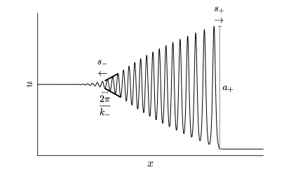
Figure 19: KdV-type DSW in convex dispersive hydrodynamics with negative dispersion. The DSW fitting relations determine the soliton edge velocity $s_{+}$ and amplitude $a_{+}$ as well as the harmonic edge velocity $s_{-}$ and wavenumber $k_{-}$.

DSW fitting relations

For non-integrable dispersive equations such as the BBM equation, diagonalization of the associated Whitham modulation system in terms of Riemann invariants is generally not possible. Thus, the explicit determination of the Whitham system’s simple wave solution corresponding to a DSW is problematic, even though its existence requires only strict hyperbolicity and genuine nonlinearity in the 2-wave characteristic family. One can, however, explicitly determine key observables associated to each DSW edge for integrable and non-integrable equations provided the dispersive hydrodynamics are convex. These observables include the DSW edge speeds $s_{\pm}$ and their associated wave parameters—the harmonic edge wavenumber $k_{-}$ and the soliton edge amplitude $a_{+},$ as functions of the initial data $u_{\pm}$. The determination of these observables represents the fitting of a DSW to the long-time dynamics of dispersive Riemann initial data. The DSW fitting method proposed in [12] (see also [16]) is based on a fundamental, generic property: the Whitham modulation equations admit exact reductions to a set of common, much simpler, analytically tractable equations in the limits of vanishing amplitude and vanishing wavenumber, which correspond to the harmonic and soliton DSW edges, respectively. DSW fitting has also been successfully applied to the propagation of a broad localized pulse into a constant state [14, 29, 36].

We now formulate the set of DSW fitting relations for an initial step in the mean $\overline{u}$, a dispersive hydrodynamic analogue of the classical Rankine-Hugoniot jump conditions for viscously regularized shocks. As outlined above, the DSW fitting relations specify the speeds $s_{-}$ and $s_{+}$ of the DSW edges and the associated wave parameters $k_{-}$ and $a_{+}$ in terms of the Riemann data $(u_{-},u_{+})$. Since we focus on positive DSW polarity and orientation, the leftmost trailing edge, propagating with constant speed $s_{-}$, is associated with the vanishing amplitude harmonic wave, while the rightmost leading edge, propagating with speed $s_{+},$ is associated with the solitary wave. Thus, $s_{+}>s_{-}$. In what follows, the Riemann step data $(u_{-},u_{+})$ of (1.7) are fixed in the regime of interest (6.1), where we assume the existence of the integral 2-wave curve of the modulation system connecting the harmonic and soliton edges. The DSW fitting relations are summarized in three steps (see [12, 16] for additional details):

(i)  The DSW harmonic edge is the modulation characteristic $x=s_{-}t$ with speed $s_{-}=s_{-}(u_{-},u_{+})$ determined by the linear group velocity for the edge mean $\overline{u}=u_{-}$ and wavenumber $k=k_{-}$:

$$s_{-}=\partial_{k}\omega_{0}(k_{-},u_{-}).$$ (6.3)

Given $u_{-}$ and $u_{+}$, the harmonic edge wavenumber $k_{-}$ is determined by solving the initial value problem

$$\frac{\mathrm{d}k}{\mathrm{d}\overline{u}}=\frac{\partial_{\overline{u}}\omega_{0}(k,\overline{u})}{f^{\prime}(\overline{u})-\partial_{k}\omega_{0}(k,\overline{u})},\quad k(u_{+})=0,$$ (6.4)

for $K(\overline{u},u_{+})\equiv k(\overline{u})$, and setting $k_{-}=K(u_{-},u_{+})$.

(ii)  The DSW soliton edge is the characteristic $x=s_{+}t$ whose speed $s_{+}=s_{+}(u_{-},u_{+})$ coincides with the solitary wave velocity for the edge mean $\overline{u}=u_{+}$ and amplitude $a=a_{+}$

$$s_{+}=c(a_{+},u_{+}),$$ (6.5)

where $c(a,\overline{u})$ is the velocity of a solitary wave with amplitude $a$ on the background $\overline{u}$. For the description of the soliton edge, it is instructive to make the change of variables $(\overline{u},a)\to(\overline{u},\tilde{k})$, where the conjugate wavenumber $\tilde{k}$ is defined implicitly by

$$c(a,\overline{u})=\frac{\tilde{\omega}_{0}(\tilde{k},\overline{u})}{\tilde{k}},$$ (6.6)

and $\tilde{\omega}_{0}(\tilde{k},\overline{u})$ is the conjugate dispersion relation defined in terms of the linear dispersion relation according to $\tilde{\omega}_{0}(\tilde{k},\overline{u})=-i\omega_{0}(i\tilde{k},\overline{u})$. Given $u_{-}$, $u_{+}$, the value $\tilde{k}_{+}$ at the soliton edge of the DSW is determined by solving the initial value problem

$$\frac{\mathrm{d}\tilde{k}}{\mathrm{d}\overline{u}}=\frac{\partial_{\overline{u}}\tilde{\omega}_{0}(\tilde{k},\overline{u})}{f^{\prime}({\overline{u}})-\partial_{\tilde{k}}\tilde{\omega}_{0}(\tilde{k},\overline{u})},\quad\tilde{k}(u_{-})=0$$ (6.7)

for $\tilde{K}(u_{-},\overline{u})\equiv\tilde{k}(\overline{u})$, and setting $\tilde{k}_{+}=\tilde{K}(u_{-},u_{+})$. The soliton edge speed $s_{+}$ and the solitary wave amplitude $a_{+}$ are then found from (6.5), (6.6), with $\tilde{k}=\tilde{k}_{+}$, $\overline{u}=u_{+}$.

Note that we have used a slightly modified presentation of DSW fitting as compared to Refs. [12, 16] in order to explicitly highlight the dependence of the edge velocities $s_{\pm}$ and edge wave parameters $k_{-}$, $a_{+}$ on the initial Riemann data $u_{-}$, $u_{+}$.

(iii)  Admissibility conditions:  The DSW fitting relations are subject to the existence of a 2-wave curve of the Whitham modulation equations continuously connecting $(\overline{u},k,a)=(u_{-},k_{-},0)$ to $(\overline{u},k,a)=(u_{+},0,a_{+})$. The following admissibility conditions are necessary for the existence of a 2-wave solution [12, 26]

Causality: $$s_{-}<f^{\prime}(u_{-}),\ \ s_{+}>f^{\prime}(u_{+}),\ \ s_{+}>s_{-}.$$ (6.8)

Convexity: $$\frac{\partial s_{-}}{\partial u_{-}}\neq 0,\quad\frac{\partial s_{-}}{\partial u_{+}}\neq 0,\quad\frac{\partial s_{+}}{\partial u_{+}}\neq 0,\quad\frac{\partial s_{+}}{\partial u_{-}}\neq 0.$$ (6.9)

DSW interior modulation

It was shown in [10] that the DSW fitting procedure can be extended into the DSW interior $x>s_{-}t$ adjacent to the harmonic edge, where the wave amplitude is small. This is done by exploiting the overlap domain for the asymptotic applicability of weakly nonlinear modulated (Stokes) waves in the Whitham modulation equations (describing slow modulations of arbitrary amplitude waves) and the nonlinear Schrödinger equation (describing slow modulations of finite but small amplitude waves). A brief outline of the results of [10] relevant to this paper is presented below.

The weakly nonlinear regime of the DSW $|u(x,t)-u_{-}|\ll u_{-}$ is well described by a slowly modulated Stokes wave

$$u(x,t)\sim u_{-}+\left[A(x,t)e^{i(k_{-}x-\omega_{0}(k_{-},u_{-})t)}+{\mathrm{c.c.}}\right]+B(x,t),$$ (6.10)

where $k_{-}=K(u_{-},u_{+})$ is determined by DSW fitting, $A(x,t)\in\mathbb{C}$ and $B(x,t)\in\mathbb{R}$ are slowly varying fields in comparison to the fast oscillations of the carrier wave. Note that $B(x,t)$ describes the induced mean flow. The crest to trough amplitude $a(x,t)$ and the wavenumber $k(x,t)=k_{-}+v(x,t)$ of the Stokes wave are related to the complex envelope $A(x,t)$ by

$$A(x,t)=\frac{a(x,t)}{4}\exp\left[i\int v(x,t)dx\right].$$ (6.11)

The dynamics of $A(x,t)$ are governed by the nonlinear Schrödinger (NLS) equation

$$iA_{t}+is_{-}A_{x}+\beta_{-}A_{xx}+\gamma_{-}|A|^{2}A=0,\quad B=b(k_{-},u_{-})|A|^{2},$$ (6.12)

where $\beta_{-}=\beta(k_{-},u_{-})=\tfrac{1}{2}\partial_{kk}\omega_{0}(k_{-},u_{-})$ and $\gamma_{-}=\gamma(k_{-},u_{-})$ are determined as part of the standard multiple scales derivation of the NLS equation (see for instance [5]). Note that the slow variation of the background $\overline{u}(x,t)$ is solely due to the induced mean flow and is constrained to the variation of the amplitude according to

$$\overline{u}=u_{-}+b_{-}a^{2}/16,$$ (6.13)

where $b_{-}=b(k_{-},\overline{u}_{-})$ is also determined as part of the NLS derivation. The NLS equation describes a stable modulation iff $\beta_{-}\gamma_{-}<0$ (defocusing regime). Also, the derivation requires that $\beta_{-}$ does not vanish, which is the case in the convex modulation regime considered here.

For the description of a DSW’s structure, the NLS equation (6.12) is considered with boundary conditions specified at the harmonic edge

$$x=s_{-}t:\qquad a(x,t)=0,\ \ k(x,t)=k_{-}.\;$$ (6.14)

As a result, the universal DSW modulation near the trailing edge is given by the following special self-similar rarefaction wave solution of (6.12)

$$a(x,t)\sim\frac{4}{3\sqrt{-2\beta_{-}\gamma_{-}}}\left[\frac{x}{t}-s_{-}\right],\;\quad k(x,t)\sim k_{-}+\frac{1}{3\beta_{-}}\left[\frac{x}{t}-s_{-}\right].$$ (6.15)

The formulae (6.15) represent a first-order approximation of the DSW’s structure near its harmonic edge. A more accurate description of the DSW modulation, which asymptotically extends deeper into the DSW’s interior, is achieved by including higher-order terms in the derivation of the NLS equation. The resulting HNLS equation (see Appendix) subject to the boundary conditions (6.14) yields a rarefaction wave solution for $a$ and $k$ that includes terms $\mathcal{O}(\frac{x}{t}-s_{-})^{2}$ in addition to the linear terms of eq. (6.15).

6.2 BBM DSW fitting

We now apply the DSW fitting relations (6.3)-(6.7) and the universal modulation formulae (6.15) (and its HNLS improvement) to the description of BBM DSWs generated within the region of Riemann data $u_{-},u_{+}$ defined by the admissibility conditions (6.8), (6.9). The BBM equation satisfies the prerequisites for DSW fitting [12, 16]: periodic travelling waves parameterised by three independent integrals of motion exist (with harmonic wave and solitary wave limits) and BBM has at least two conservation laws (1.4) and (5.11). The speed-amplitude relation for solitary waves is given by (5.2). We initially consider the Riemann data (1.6) with $u_{-}>u_{+}>0$ (other configurations will be considered later).

Using the BBM linear dispersion relation (3.2), the characteristic equation (6.4) for the harmonic edge is

$$\frac{\mathrm{d}k}{\mathrm{d}\overline{u}}=\frac{1+k^{2}}{\overline{u}k(3+k^{2})},\quad k(u_{+})=0.$$ (6.16)

Integration yields

$$\overline{u}=u_{+}(1+k^{2})e^{k^{2}/2}.$$ (6.17)

The $k$-locus $k_{-}=K(u_{-},u_{+})$ at the DSW harmonic edge is then found from (6.17) by setting $\overline{u}=u_{-}$, $k=k_{-}$, and is given by the implicit equation

$$(1+k_{-}^{2})e^{k_{-}^{2}/2}=\frac{u_{-}}{u_{+}}\,.$$ (6.18)

The harmonic edge speed is then found from (3.3) as

$$s_{-}=\partial_{k}\omega_{0}(k_{-},u_{-})=u_{-}\frac{1-k_{-}^{2}}{(1+k_{-}^{2})^{2}}.$$ (6.19)

To describe the solitary wave edge, we introduce the BBM conjugate dispersion relation $\tilde{\omega}_{0}(\tilde{k},\overline{u})=-i\omega_{0}(i\tilde{k},\overline{u})$ to obtain

$$\tilde{\omega}_{0}(\tilde{k},\overline{u})=\overline{u}\frac{\tilde{k}}{1-\tilde{k}^{2}}.$$ (6.20)

The characteristic equation (6.7) for the solitary wave edge then becomes

$$\frac{\mathrm{d}\tilde{k}}{\mathrm{d}\overline{u}}=\frac{1-\tilde{k}^{2}}{\overline{u}\tilde{k}(\tilde{k}^{2}-3)},\quad\tilde{k}(u_{-})=0.$$ (6.21)

Its solution has the form

$$\overline{u}=u_{-}(1-\tilde{k}^{2})e^{-\tilde{k}^{2}/2}$$ (6.22)

The $\tilde{k}$-locus $\tilde{k}_{+}=\tilde{K}(u_{-},u_{+})$ of the DSW soliton edge is obtained by setting $\overline{u}=u_{+}$, $\tilde{k}=\tilde{k}_{+}$ in (6.22), and is given by the implicit equation (cf. (6.18))

$$(1-\tilde{k}_{+}^{2})e^{-\tilde{k}_{+}^{2}/2}=\frac{u_{+}}{u_{-}}.$$ (6.23)

The solitary wave edge speed $s_{+}$ is found from (6.5), (6.6) by setting $\tilde{k}=\tilde{k}_{+}$, $\overline{u}=u_{+}$:

$$s_{\rm+}=\frac{\tilde{\omega}_{0}(\tilde{k}_{+},u_{+})}{\tilde{k}_{+}}=\frac{u_{+}}{1-\tilde{k}_{+}^{2}}\,.$$ (6.24)

The DSW amplitude $a_{+}$ at the soliton edge is then determined via $s_{\rm+}=c(a_{+},u_{+})$ with $c(a,\overline{u})$ given by (5.2), which yields

$$a_{+}=3u_{+}\frac{\tilde{k}_{+}^{2}}{1-\tilde{k}_{+}^{2}}.$$ (6.25)

Positivity of the solitary wave amplitude requires $\tilde{k}_{+}<1$.

We now verify the DSW fitting admissibility conditions (6.8), (6.9). The first two causality conditions (6.8) for BBM assume the form $s_{-}<u_{-},\ \ s_{+}>u_{+}$ and are readily verified provided $\tilde{k}_{+}<1$, which is true so long as $u_{-}>u_{+}>0$. Next, a calculation yields

$$\frac{\partial s_{-}}{\partial u_{-}}=-\frac{3+k_{-}^{4}}{(1+k_{-}^{2})^{2}(3+k_{-}^{2})},\quad\frac{\partial s_{-}}{\partial u_{+}}=\frac{2(3-k_{-}^{2})e^{k_{-}^{2}/2}}{3+4k_{-}^{2}+k_{-}^{4}}.$$ (6.26)

While the first convexity condition in (6.9) is always satisfied, the second condition requires $k_{-}\neq\sqrt{3}$, which, after substitution in (6.18), gives $({u_{-}}/{u_{+}})\neq 4e^{3/2}$. The critical line

$$u_{+}=\mu\,u_{-},\quad\mu=e^{-3/2}/4\approx 0.056$$ (6.27)

corresponds to the zero dispersion point $k_{-}=\sqrt{3}$ and delimits the applicable region for the DSW fitting method

$$0<\mu u_{-}<u_{+}.$$ (6.28)

Another calculation yields

$$\frac{\partial s_{+}}{\partial u_{+}}=\frac{1}{3-\tilde{k}_{+}^{2}},\quad\frac{\partial s_{+}}{\partial u_{-}}=\frac{2e^{-\tilde{k}_{+}^{2}/2}}{3-\tilde{k}_{+}^{2}}.$$ (6.29)

Equation (6.23) implies that $0<\tilde{k}_{+}<1$ within the region (6.28). Then the third and fourth convexity conditions in (6.9) are readily verified to hold true for all $u_{-},u_{+}$ in (6.28).

It follows that within the admissibility region (6.28), $k_{-}<\sqrt{3}$ so the dispersion sign is

$$\mathrm{sgn}\,\beta(k_{-},u_{-})=\mathrm{sgn}\left(u_{-}\frac{2k_{-}(k_{-}^{2}-3)}{(1+k_{-}^{2})^{3}}\right)<0.$$ (6.30)

Consequently, the DSW orientation and polarity are $d=p=1$, consistent with our original assumption $s_{+}>s_{-}$, which ensures the third causality condition (6.8) within the region (6.28) for $\mu$ defined in (6.27).

Figure 20(a) shows excellent agreement between the analytical expressions (6.19) and (6.24) and the velocities of the DSW edges extracted from numerical simulations. Additionally, Fig. 20(b) displays the comparison between (6.18) and the harmonic edge wavenumber extracted numerically, and Fig. 20(c) displays the comparison between (6.25) and the solitary wave edge amplitude.

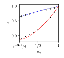
(a) Edge velocities (6.19) and (6.24).

(b) Harmonic edge wavenumber (6.18).

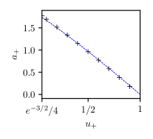
(c) Solitary wave edge amplitude (6.25).

Figure 20: Edge parameters as functions of $u_{+}$ for fixed $u_{-}=1$. Solid (resp. dashed) lines represent DSW fitting formulas for the harmonic (resp. solitary wave) edge. Markers represent the parameter values extracted from direct numerical simulation of the BBM smoothed dispersive Riemann problem at $t=1000$ with initial data (1.7) where $\xi=10$.

The interior BBM DSW modulation in the vicinity of the harmonic edge is given by (6.15). It is determined by the coefficients $\beta(k,\overline{u})$ and $\gamma(k,\overline{u})$ of the NLS equation (6.12) for slowly varying modulations of the weakly nonlinear periodic traveling wave of the BBM equation with $k=k_{-}$, $\overline{u}=u_{-}$. The derivation of the NLS equation is standard and we only present here the expressions for $\beta$ and $\gamma$

$$\beta(k,\overline{u})=\overline{u}\frac{k(k^{2}-3)}{(1+k^{2})^{3}},\;\quad\gamma(k,\overline{u})=\frac{3+5k^{2}}{6\overline{u}k(3+k^{2})}.$$ (6.31)

Within the admissible region (6.28), $k_{-}<\sqrt{3}$ and so $\beta(k_{-},u_{-})\gamma(k_{-},u_{-})<0$, thus ensuring modulational stability of the DSW’s harmonic edge. Additionally, the function $b(k,\overline{u})$ determining the variation of the induced mean flow (6.13) near $x=s_{-}t$ is given by

$$b(k,\overline{u})=-\frac{(1+k^{2})^{2}}{\overline{u}k^{2}(3+k^{2})}.$$ (6.32)

A comparison between the modulation solution (6.15), (6.13), and the DSW structure extracted from numerical simulations is displayed in Fig. 21. The figure also displays the modulation solution obtained using the HNLS approximation, see Appendix B and [10] for details. The HNLS modulation solution provides the best agreement with the numerical DSW structure near the harmonic edge and deeper into the DSW interior. Near the soliton edge, there is a departure from the HNLS description, which is to be expected because the (H)NLS descriptions are based upon modulations of a weakly nonlinear Stokes wave, which does not describe the DSW in the strongly nonlinear, or solitary wavetrain regime.

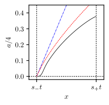
(a) amplitude

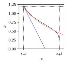
(b) wavenumber

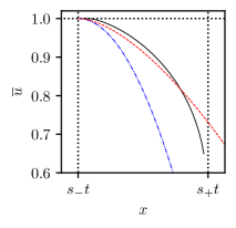
(c) mean value

Figure 21: Comparison between the asymptotic prediction for the DSW structure and the numerical solution of the smoothed dispersive Riemann problem (1.4), (1.7) at $t=1000$ with $(u_{-},u_{+},\xi)=(1,0.2,10)$. The black solid line is the numerical solution, the dash-dotted blue line is the NLS prediction and the dashed red line is the HNLS prediction.

The wavenumber and mean value predictions in Figures 21(b), 21(c) visually exhibit better agreement with the numerically extracted DSW parameters than the DSW amplitude in 21(a). There is some deviation in the numerically extracted oscillation envelope amplitude depicted in Fig. 21(a) near the trailing edge from predicted linear behavior $a\propto\frac{x}{t}-s_{-}$ in (6.15). This is not surprising given that our analysis in Section 3 demonstrates that the transition width for smoothed step initial data significantly alters the DSW’s oscillatory structure in the neighborhood of the DSW harmonic edge. In fact, a fundamental discrepancy between the DSW modulation solution and the numerical oscillation behavior is known and even occurs for the KdV equation [22]. In contrast to the well-defined DSW soliton edge, the DSW harmonic edge discrepancy from leading order modulation theory leads to ad hoc approaches for comparing the harmonic edge velocity and wavenumber with numerical simulations. Nevertheless, modulation theory provides a reasonable prediction of the DSW’s amplitude, wavenumber, and mean structure near the DSW harmonic edge.

6.3 DSW implosion

Figure 22 shows that the solution of the dispersive Riemann problem is no longer a single-phase DSW when $u_{+}<\mu u_{-}$. A beating pattern develops close to the DSW small-amplitude edge that is clearly depicted in the examples for which $u_{+}\leq-0.3$. This phenomenon has been previously identified [35] as DSW implosion in which the group velocity of linear waves at the harmonic edge experiences a minimum, i.e. at a zero dispersion point. In this section, we investigate the solution for $u_{+}<\mu u_{-}$ in greater detail. In the numerical examples presented in this section, $\xi=10$ unless otherwise stated. The variation of a typical solution when $u_{+}=-0.5$ in Fig. 22 shows that 3 distinct modulation regions exist: a finite amplitude, stable, single-phase wave in region I, a beating pattern in region II and a small amplitude wave in region III; the boundaries between regions I and II denoted $x=x_{\rm b}$, and regions II and III denoted $x=x_{\rm a}$, separate the spatial regions where the wave is single-phase and two-phase.

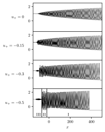
(a) Variation of the whole solution.

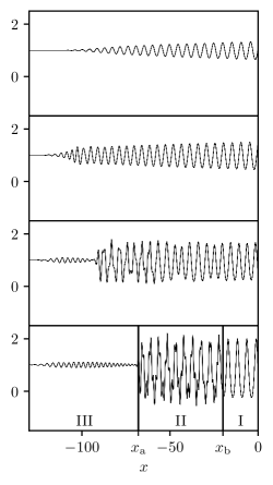
(b) Close up of the region: $x<0$.

Figure 22: Numerical solution of the dispersive Riemann problem with $u_{+}\leq 0<u_{-}=1$ at $t=1000$. When $u_{+}\ll\mu u_{-}$, the solution divides into three distinct regions identified in the example $u_{+}=-0.5$. Vertical solid lines correspond to the left and right boundaries of region II: $x=x_{\rm a}(t)$ and $x=x_{\rm b}(t)$.

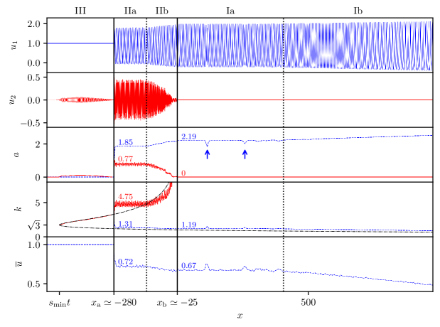
Figure 23: Variation of the slow and fast oscillatory fields $u_{1}$ and $u_{2}$, respectively, extracted from the numerical solution $u(x,t)$ at $t=4000$ when $(\xi,u_{-},u_{+})=(10,1,-0.5)$. Variation of the fields $u_{1}$, $u_{2}$ are displayed in the first, second rows with dashed, solid curves, respectively. Their extracted amplitude $a_{1},a_{2}$ and wavenumber $k_{1},k_{2}$ modulations are shown in the third and fourth rows, respectively with dashed (resp. solid) curves corresponding to parameters for the field $u_{1}$ (resp. $u_{2}$). The dash-dotted curve in the fourth row is the linear, stationary phase solution (3.14),(3.15). The fifth row depicts the mean of the solution $\bar{u}$. Solid vertical lines represent the boundaries $x_{\rm a}$ and $x_{\rm b}$ and dash-dotted vertical lines identify internal subdivisions of regions I (Sec. 6.3.1) and II (Sec. 6.3.2). Vertical arrows indicate the position of dark solitary waves in region Ia.

6.3.1 Region I: stable single-phase wave

We first consider the modulation of the wave in region I. The variations of the crest to trough amplitude $a(x,t)$, the wavenumber $k(x,t)$, and the mean $\overline{u}(x,t)$ obtained numerically are displayed in Fig. 23 (where $u_{1}=u$ in region I, as detailed in Sec. 6.3.2). Region I can be subdivided into two subregions: a region denoted Ia where $a(x,t)$, $k(x,t)$, and $\bar{u}(x,t)$ are approximately constant, apart from localized, small-width modulations, and a region denoted Ib where $a(x,t)$, $k(x,t)$, and $\overline{u}(x,t)$ vary monotonically. The modulation in region Ib is similar to the DSW modulation investigated in Secs. 6.1 and 6.2 where the wavenumber $k(x,t)$ monotonically decreases until it reaches the solitary wave limit $k=0$, while the amplitude monotonically increases toward the soliton edge. However, the DSW fitting of Sec. 6.1 does not apply to this region since the admissibility condition (6.28) is not fulfilled, and the parameters of the soliton edge cannot be obtained using this method. In fact, the wave structure in region Ib can be identified as a partial DSW, where the nonlinear modulated wave does not reach the small-amplitude, harmonic limit. Instead, it terminates at some nonzero amplitude $a_{0}$, mean $\bar{u}_{0}$, and wavenumber $\kappa_{0}$ that are matched to the right edge of region Ia. These types of structures occur in initial-boundary value problems for nonlinear dispersive PDEs (see, e.g. [38]) and, in particular, are realized in problems involving resonant or transcritical shallow-water flows past localized bathymetry [24, 44, 13]. We do not present a quantitative description of partial BBM DSWs here as this would require the development of a full nonlinear modulation theory for the BBM equation, a significant undertaking that deserves a dedicated study.

The specific modulation of the wave in region Ia is a new feature that only develops when $\sigma_{3}u_{-}<u_{+}<\mu u_{-}$. The localized depletions of the amplitude $a(x,t)$ and the corresponding augmentations of the wavenumber $k(x,t)$ propagate on the “background” $(a,k)=(a_{0},\kappa_{0})$ at constant velocity; we have, for instance in the example of Fig. 23 where $u_{+}=-0.5$, $(a_{0},\kappa_{0})\approx(2.19,1.19)$. In the following, we investigate the modulation of the field $u(x,t)$ using a weakly nonlinear NLS description that was introduced in the previous sections. The nonlinear wave can be approximated in the weakly nonlinear regime by the Stokes wave (cf. for instance (6.10))

$$u(x,t)\sim\overline{u}(x,t)+\left[A(x,t)e^{i(\kappa_{0}x-\omega_{0}(\kappa_{0},u_{-})t)}+{\mathrm{c.c.}}\right],$$ (6.33)

where $\overline{u}(x,t)\sim u_{-}$ is a slowly varying field. The crest to trough amplitude $a$ and the wavenumber $k$ are given by

$$a(x,t)=4|A(x,t)|,\;k(x,t)=\kappa_{0}+\partial_{x}\arg A.$$ (6.34)

Since $\kappa_{0}<\sqrt{3}$, the complex envelope of the Stokes wave $A(x,t)$ solves the defocusing NLS equation ($\beta(\kappa_{0},u_{-})\gamma(\kappa_{0},u_{-})<0$):

$$iA_{t}+i\partial_{k}\omega_{0}(\kappa_{0},u_{-})A_{x}+\beta(\kappa_{0},u_{-})A_{xx}+\gamma(\kappa_{0},u_{-})|A|^{2}A=0.$$ (6.35)

We first consider the nonlinear plane wave solution

$$a=a_{0}={\rm const},\quad k=\kappa_{0}={\rm const}.$$ (6.36)

Substituting (6.36) into the NLS equation (6.35), we obtain the modulation of the complex envelope

$$A(x,t)=\frac{a_{0}}{4}\exp\left(i\Delta\omega_{0}t\right),\quad\Delta\omega_{0}=\gamma(\kappa_{0},u_{-})\frac{a_{0}^{2}}{16}.$$ (6.37)

As a result, the weakly nonlinear wave in region Ia is approximately

$$u(x,t)=\overline{u}+\frac{a_{0}}{4}\cos\left[\kappa_{0}x-(\omega_{0}(\kappa_{0},u_{-})-\Delta\omega_{0})t\right],\quad\overline{u}=u_{-}+b(\kappa_{0},u_{-})\frac{a_{0}^{2}}{16}$$ (6.38)

showing that weakly nonlinear interaction shifts the linear frequency $\omega_{0}(\kappa_{0},u_{-})$ by $-\Delta\omega_{0}$. Figure 24(a) displays the frequency shift computed numerically for the example $u_{+}=-0.5$, and shows reasonable agreement with the NLS equation description (6.35). Equation (6.38) also yields $\overline{u}=0.77$ whereas the average extracted numerically is $\overline{u}\approx 0.67$ as shown in Fig. 23. A better analytical approximation of $\Delta\omega_{0}$ and $\overline{u}$ necessitates higher order terms in the NLS description.

(a) $x=0$ (region Ia)

(b) $x=-300$ (region IIa)

Figure 24: Temporal Fourier transform of the numerical solution $u(x,t)-u_{-}$ [$(u_{-},u_{+},\xi)=(1,-0.5,10)$] at a fixed position $x$ and the time-sampling $t\in(5000,6000)$. Peaks of the Fourier transform indicate the dominant frequency of the weakly nonlinear wave. Dashed vertical lines indicate the linear frequencies $\omega_{0}(\kappa_{i})$ and solid vertical lines the shifted frequencies $\omega_{0}(\kappa_{i})-\Delta\omega_{i}$.

Localized perturbations of the parameters $a(x,t)$ and $k(x,t)$ can be identified with dark solitary wave solution of the NLS equation (6.35)

$$A_{\rm DS}(x,t)=\frac{a_{0}}{4}\left(i\,c\,\sqrt{\frac{8}{-\beta_{0}\gamma_{0}a_{0}^{2}}}+\sqrt{1+\frac{8c^{2}}{\beta_{0}\gamma_{0}a_{0}^{2}}}\tanh\left[\sqrt{-\frac{\gamma_{0}a_{0}^{2}}{32\beta_{0}}-\frac{c^{2}}{4\beta_{0}^{2}}}(x-ct-x_{0})\right]\right){\rm e}^{ia_{0}^{2}t/16},$$ (6.39)

where $\beta_{0}=\beta(\kappa_{0},u_{-})$ and $\gamma_{0}=\gamma(\kappa_{0},u_{-})$ (cf. (6.31)). The dark solitary wave is parameterized by the speed of the solitary wave $c$ and $x_{0}$, its position at $t=0$. The phase of the dark solitary wave experiences a shift when the localized amplitude depression is traversed

$$\lim_{x\to+\infty}\arg A_{\rm DS}(x,t)-\lim_{x\to-\infty}\arg A_{\rm DS}(x,t)=-2{\rm sgn}(\beta_{0}c)\cos^{-1}\left(\frac{4c}{\sqrt{-2\beta_{0}\gamma_{0}a_{0}^{2}}}\right).$$ (6.40)

This phase-shift can be observed in the numerical solution but differs from the analytical formula (6.40). This indicates that the wave in region I is governed by the NLS equation only to a first approximation, and the description of traveling waves of the envelope $A(x,t)$ necessitates a higher order description such as the HNLS equation (B.2). We leave this comparison as a subject for future work.

The emergence of envelope solitary waves is reminiscent of the shedding of solitary waves investigated in Sec. 5 because solitary waves are only generated for a sufficiently large jump $|u_{-}-u_{+}|$.

6.3.2 Region II: stable two-phase wave

Figure 22 shows that the implosion of the DSW occurs in regions II and III, which broadly overlap with the two-phase region $x\in(s_{\rm min}t,0)$ identified in the linear analysis of Sec. 3. In this section, we focus on region II. We show that $u(x,t)$ displays a beating pattern that can be approximated by a superposition of two single-phase, weakly nonlinear waves

$$u(x,t)\sim u_{1}(x,t)+u_{2}(x,t),$$ (6.41)

were $u_{1}$ and $u_{2}$ correspond, respectively, to slow and fast oscillating waves.

In order to determine $u_{1}$ and $u_{2}$ from our numerical simulations, we compute the spatial Fourier transform of $u_{\rm II}(x,t)$, which is the restriction of $u(x,t)$ to region II. The example $u_{+}=-0.5$ is shown in Fig. 25 depicting multiple maxima of the Fourier transform. The two largest spectral contributions correspond to the dominant wavenumber $\kappa_{1}$ of the slowly oscillating wave $u_{1}$ and the dominant wavenumber $\kappa_{2}>\kappa_{1}$ of the fast oscillating wave $u_{2}$. Other maxima correspond to harmonics that result from weakly nonlinear interactions such as second harmonic generation at $2\kappa_{1}$ and $2\kappa_{2}$, and two wave interaction $\kappa_{2}\pm\kappa_{1}$. We then identify the small-wavenumber content of the Fourier spectrum ($k<k_{\rm c}$) as the Fourier transform of $u_{1}(x,t)$ and the large-wavenumber content as the Fourier transform of $u_{2}(x,t)$, where $k_{\rm c}$ is the minimum identified for $\kappa_{1}<k<\kappa_{2}$ ($k_{\rm c}\approx 2.8$ in the example depicted in Fig. 25). The variation of the fields $u_{1}$ and $u_{2}$ is obtained by computing the inverse Fourier transforms of the band limited functions

$$u_{1}(x,t)={\cal F}^{-1}\left[\begin{cases}{\cal F}[u_{\rm II}(x,t)],&k<k_{\rm c}\\ 0,&k\geq k_{\rm c}\end{cases}\right],\quad u_{2}(x,t)={\cal F}^{-1}\left[\begin{cases}0,&k<k_{\rm c}\\ {\cal F}[u_{\rm II}(x,t)],&k\geq k_{\rm c}\end{cases}\right].$$ (6.42)

The division into small and large wavenumber bands of the Fourier spectrum was examined in Sec. 3 for linear waves. There, $k_{\rm c}=\sqrt{3}$ separated the small and large wavenumber bands. In the weakly nonlinear regime, $k_{\rm c}\neq\sqrt{3}$ because the second harmonic $2\kappa_{1}$ can be larger than $\sqrt{3}$ ($2\kappa_{1}\simeq 2.6$ in the example presented in Fig. 25). The variation of $u_{1}(x,t)$ and $u_{2}(x,t)$ extracted from the numerical solution for $u_{-}=-0.5$ and their modulation parameters in region II are depicted in Fig. 23. Note that the numerical method presented here to extract the two single-phase waves only yields an approximation to $u_{1}$ and $u_{2}$. For instance, the higher harmonic $\kappa_{2}-\kappa_{1}$ contributes to the Fourier spectrum of $u_{2}$ in the example considered in Fig. 25, even though it corresponds to the nonlinear interaction between $u_{1}$ and $u_{2}$. In practice, the quasi-monochromatic aspect of the extracted waves $u_{1}$ and $u_{2}$ (cf. Fig. 23) indicates that the numerical method presented above yields a good approximation.

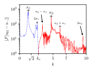
Figure 25: Fourier transform of $u_{\rm II}(x,t)-u_{-}$ for $(\xi,u_{-},u_{+})=(10,1,-0.5)$ at $t=4000$. $k_{\rm c}\sim 2.83$ divides the spectrum in a small-wavenumber region (dashed blue line) and large-wavenumber region (solid red line). The crosses $+$ identified the dominant wavenumbers of the component $u_{1}$ and $u_{2}$ as well as the corresponding higher order harmonics.

We now make the ansatz that the two modulated wavetrains $u_{1}$ and $u_{2}$ can be modeled by two Stokes waves

$$\begin{split}u_{1}(x,t)=\left[A_{1}(x,t)e^{i(\kappa_{1}x-\omega_{0}(\kappa_{1},u_{-})t)}+{\mathrm{c.c.}}\right]+\overline{u}(x,t),\;u_{2}(x,t)=A_{2}(x,t)e^{i(\kappa_{2}x-\omega_{0}(\kappa_{2},u_{-})t)}+{\mathrm{c.c.}},\\ \end{split}$$ (6.43)

where $A_{1}(x,t),A_{2}(x,t)$ are complex valued and $\overline{u}(x,t)$ is real valued, all of which are slowly varying. The dominant wavenumbers of the Stoke waves satisfying $\kappa_{1}<\sqrt{3}$ and $\kappa_{2}>\sqrt{3}$ are extracted numerically using the procedure already described. Note that by the definition of $u_{1}$ and $u_{2}$, the slow modulation of the background $\overline{u}(x,t)$ is necessarily incorporated in the variation of $u_{1}(x,t)$ so that $u_{2}(x,t)$ has zero mean. The crest to trough amplitudes $a_{j}$ and wavenumbers $k_{j}$ are

$$a_{j}(x,t)=4|A_{j}(x,t)|,\quad k_{j}(x,t)=\kappa_{j}+\partial_{x}\arg A_{j},\quad j=1,2.$$ (6.44)

The modulation equations for the complex envelopes $A_{1}$ and $A_{2}$ are two coupled NLS equations

$$\begin{split}&iA_{1t}+i\partial_{k}\omega_{0}(\kappa_{1},u_{-})A_{1x}+\beta(\kappa_{1},u_{-})A_{1xx}+\left[\gamma(\kappa_{1},u_{-})|A_{1}|^{2}+\nu(\kappa_{1},\kappa_{2},u_{-})|A_{2}|^{2}\right]A_{1}=0,\\ &iA_{2t}+i\partial_{k}\omega_{0}(\kappa_{2},u_{-})A_{2x}+\beta(\kappa_{2},u_{-})A_{2xx}+\left[\gamma(\kappa_{2},u_{-})|A_{2}|^{2}+\nu(\kappa_{2},\kappa_{1},u_{-})|A_{1}|^{2}\right]A_{2}=0,\\ &\overline{u}(x,t)=u_{-}+b(\kappa_{1},u_{-})|A_{1}|^{2}+b(\kappa_{2},u_{-})|A_{2}|^{2},\end{split}$$ (6.45)

obtained with a standard multiple-scale computation. The coefficients $\beta(\kappa,u_{-})$ and $\gamma(\kappa,u_{-})$ are given in (6.31) and $b(\kappa,u_{-})$ in (6.32). The nonlinear interaction between the two components $A_{1}$ and $A_{2}$ is characterized by the coefficient

$$\nu(\kappa,\lambda,u_{-})=\frac{\kappa(1+\lambda^{2})(9+6\kappa^{2}+\kappa^{4}+21\lambda^{2}+13\kappa^{2}\lambda^{2}+\kappa^{4}\lambda^{2}+9\lambda^{4}+3\kappa^{2}\lambda^{4}+\lambda^{6})}{(1+\kappa^{2})\lambda^{2}(3+\lambda^{2})(3+\kappa^{2}-\kappa\lambda+\lambda^{2})(3+\kappa^{2}+\kappa\lambda+\lambda^{2})u_{-}}>0.$$ (6.46)

The modulation description (6.43), (6.45) is the weakly nonlinear extension of the modulated two-phase linear wave solution (3.18), which applies when the two wavenumbers $k_{1}$ and $k_{2}$ are distinct.

As indicated in Fig. 23, Region II can be divided into two subregions: region IIa where the wave parameters are approximately constant, and region IIb where the variations of $a_{j}(x,t)$, $j=1,2$ are approximately monotone.

We first focus on the modulation in region IIb where the amplitudes $a_{1}(x,t)$ and $a_{2}(x,t)$ are, respectively increasing and decreasing functions of $x$. Ultimately $a_{2}(x,t)=0$ at the boundary with region I ($x=x_{\rm b}$) and the amplitude of the slow varying wave $a_{1}(x,t)$ matches with $a(x,t)=a_{0}$ in region Ia. We thus extend the definition of $u_{1}$ and $u_{2}$ to region I by setting:

$$u_{1}(x,t)=u(x,t),\quad u_{2}(x,t)=0,\quad\forall x\geq x_{\rm b}.$$ (6.47)

The modulation close to $x=x_{\rm b}$ can thus be uniformly described, across the boundary between the region IIb and Ia, by the simplified coupled equations

$$\begin{split}&iA_{1t}+i\partial_{k}\omega_{0}(\kappa_{1},u_{-})A_{1x}+\beta(\kappa_{1},u_{-})A_{1xx}+\gamma(\kappa_{1},u_{-})|A_{1}|^{2}A_{1}=0,\\ &iA_{2t}+i\partial_{k}\omega_{0}(\kappa_{2},u_{-})A_{2x}+\beta(\kappa_{2},u_{-})A_{2xx}+\nu(\kappa_{2},\kappa_{1},u_{-})|A_{1}|^{2}A_{2}=0.\end{split}$$ (6.48)

The approximation of (6.45) invoked here is $|A_{2}|\ll|A_{1}|$, as suggested by Fig. 23. The modulation of $A_{1}$ is independent of $A_{2}$ and is governed by the, modulationally stable, defocusing NLS equation as described in Sec. 6.3.1. The modulation of $A_{2}$ is a linear Schrödinger equation with potential $-\nu(\kappa_{2},\kappa_{1},u_{-})|A_{1}(x,t)|^{2}$. Consequently, although the wavenumber $\kappa_{2}$ is larger than $\sqrt{3}$, the modulation dynamics of $u_{2}$ remain stable in the vicinity of $x=x_{\rm b}$. This highlights the stabilizing effect of the slowly-oscillating component $u_{1}(x,t)$ on the fast-oscillating component $u_{2}(x,t)$ in region IIb. We do not carry out a detailed analysis of the modulations $A_{j}$ in region IIb, leaving that for a separate, dedicated study.

We now consider region IIa for which the modulation variables are approximately constant

$$a_{1}={\rm const},\quad a_{2}={\rm const},\quad k_{1}=\kappa_{1},\quad k_{2}=\kappa_{2},$$ (6.49)

where we identify the modulation wavenumber $k_{j}$ with the constant, dominant wavenumber $\kappa_{j}$ extracted from the numerical simulation so that $\partial_{x}\arg A_{j}=0$. The values of the parameters $a_{j}$ are also extracted from the numerical solution. In Fig. 23, we have $(a_{1},k_{1})\approx(1.85,1.31)$ and $(a_{2},k_{2})\approx(0.77,4.75)$. Substituting (6.49) into the coupled NLS equations (6.45), we obtain the modulation of the complex envelopes in the form of two plane waves

$$\begin{split}&A_{1}(x,t)=\frac{a_{1}}{4}\exp\left(i\Delta\omega_{1}t\right),\quad\Delta\omega_{1}=\frac{1}{16}\left(\gamma(\kappa_{1},u_{-})a_{1}^{2}+\nu(\kappa_{1},\kappa_{2},u_{-})a_{2}^{2}\right),\\ &A_{2}(x,t)=\frac{a_{2}}{4}\exp\left(i\Delta\omega_{2}t\right),\quad\Delta\omega_{2}=\frac{1}{16}\left(\gamma(\kappa_{2},u_{-})a_{2}^{2}+\nu(\kappa_{2},\kappa_{1},u_{-})a_{1}^{2}\right).\end{split}$$ (6.50)

As a result, the two-phase weakly nonlinear wave in region IIa for the BBM equation is approximately

$$\begin{split}&u(x,t)=\overline{u}+\frac{a_{1}}{4}\cos\left[\kappa_{1}x-(\omega_{0}(\kappa_{1},u_{-})-\Delta\omega_{1})t\right]+\frac{a_{2}}{4}\cos\left[\kappa_{2}x-(\omega_{0}(\kappa_{2},u_{-})-\Delta\omega_{2})t\right],\\ &\overline{u}=u_{-}+b(\kappa_{1},u_{-})\frac{a_{1}^{2}}{16}+b(\kappa_{2},u_{-})\frac{a_{2}^{2}}{16}\end{split}$$ (6.51)

showing that weakly nonlinear interactions between the two wave modes shift the linear frequencies $\omega_{0}(\kappa_{1},u_{-})$ and $\omega_{0}(\kappa_{2},u_{-})$ by $-\Delta\omega_{1}$ and $-\Delta\omega_{2}$, respectively. Figure 24(b) displays good agreement between the weakly nonlinear frequency predictions (6.38) and the temporal Fourier spectrum of the BBM numerical simulation at $x=-300$ for the case $u_{+}=-0.5$. Equation (6.51) also yields $\overline{u}=0.86$ whereas the average extracted numerically in Fig. 23 is $\overline{u}\approx 0.72$. A better approximation of $\Delta\omega_{1}$, $\Delta\omega_{2}$ and $\overline{u}$ could be achieved with higher order terms in the NLS description.

It is important to point out that, in the absence of two-phase coupling, the modulation $A_{2}$ satisfies the scalar NLS equation (6.35) with $\kappa_{0}\to\kappa_{2}$. Since $\kappa_{2}>\sqrt{3}$, $\beta(\kappa_{2},u_{-})\gamma(\kappa_{2},u_{-})>0$ so that the equation is of focusing type and the plane wave solution (6.36) (with $a_{0}\to a_{2}$) for $A_{2}$ is linearly unstable to infinitesimal, long wavelength perturbations, also known as modulationally unstable. However, the nonlinear coupling between the modulations in the coupled NLS equations (6.45) can stabilize the plane wave solution (6.50). For the specific example shown in region IIa of Fig. 23, we have verified that this is indeed the case with a calculation described in Appendix C.

6.3.3 Region III: linear wave

Since the carrier wavenumber of the field $u(x,t)$ is larger than $\sqrt{3}$ in region III—cf. Fig. 23 where $(u_{1},u_{2})=(u_{-},u-u_{-})$ in region III—$u$ represents a fast oscillating wave according to the criterion introduced in Sec. 6.3.2, and we set

$$u_{1}(x,t)=u_{-},\quad u_{2}(x,t)=u(x,t),\quad\forall x<x_{\rm a}.$$ (6.52)

Contrary to the neighborhood of the boundary $x=x_{\rm b}$, the fields $u_{1}$ and $u_{2}$ are rapidly changing at the boundary $x=x_{\rm a}$.

The amplitude of $u(x,t)$ in region III is small and its modulation can be described by the linear theory introduced in Sec. 3. The bottom row of Fig. 23 shows that the modulation of the wavenumber $k(x,t)$ obtained numerically lies on the stationary point $k_{2}(x/t)$ from linear theory given by (3.15).

6.3.4 Summary of DSW implosion

Here we summarize our description of DSW implosion for dispersive Riemann problems with $\sigma_{3}u_{-}<u_{+}<\mu u_{-}$ in regions c and f of Figs. 1 and 2, respectively ($\sigma_{3}$ is defined in the next subsection). The entire coherent wave structure arises due to compressive initial data that cannot be resolved by an admissible DSW alone. Instead, both short and long waves are generated that represent a nonlinear generalization of the two-phase, linear wave modulation investigated in Sec. 3. From right to left, the solution is described by modulated long waves in a partial DSW (region I) that transitions to region II where long and short waves coexist, significantly influencing one another. This two-phase modulation abruptly terminates at a short wavelength, linear wavepacket (region III) propagating on the background $u_{-}$, hence the entire structure transitions from modulated, long nonlinear waves to modulated, short linear waves.

Similar to region I identified in linear theory, the nonlinear wave in region I is a modulated one-phase wave with a small wavenumber ($k<\sqrt{3}$). The one-phase wave in region Ib is a partial DSW, a carryover from dispersive Riemann problems with $\mu u_{-}<u_{+}<u_{-}$ in which DSWs are admissible. Its wave parameters $a$, $k$, and $\overline{u}$ are strictly monotone functions of $x$ in this region. Adjacent to the partial DSW is a stable nonlinear plane wave with multiple localized, depression modulations of the wave envelope (dark envelope solitary waves) that stably propagate in region Ia.

The wavetrain in region Ia matches smoothly to a nonlinear beating pattern in region II at $x=x_{\rm b}$. In a first approximation, $u(x,t)$ is the superposition of two modulated, weakly nonlinear, monochromatic (Stokes) waves $u_{1}(x,t)$ and $u_{2}(x,t)$, each with distinct dominant wavenumbers $\kappa_{1}<\sqrt{3}$ and $\kappa_{2}>\sqrt{3}$. This is a generalization of the superposition of two modulated, linear wavetrains with distinct dominant wavenumbers (see region II described in Sec. 3). The weakly nonlinear components $u_{1}$ and $u_{2}$ are approximately governed by coupled NLS equations, as demonstrated by their nonlinear frequency shifts. Although a weakly nonlinear wave of dominant wavenumber larger than $\sqrt{3}$ is modulationally unstable, the component $u_{2}(x,t)$ is shown to be stable when nonlinearly coupled to $u_{1}(x,t)$.

Region III displays a principal difference from linear theory. In the linear theory, the two wavenumbers $k_{1}$ and $k_{2}$ coalesce at $\sqrt{3}$ when $x=-u_{-}/8t$, and the corresponding linear wave $u(x,t)$ continuously changes from a beating two-wave structure to an Airy wave. In the dispersive Riemann problem considered here, the modulation changes very rapidly, in fact, discontinuously on the modulation length scale at $x=x_{\rm a}$. The adjacent wave in region III is a linear, one-phase wave with wavenumber $k_{2}>\sqrt{3}$. The discontinuity at $x=x_{\rm a}$ displayed in Fig. 23 resembles a so-called Whitham shock wave structure that was recently identified and investigated for several nonlinear dispersive PDEs in [46]. Higher order dispersion was shown to be essential for the generation of Whitham shocks. The coupled NLS equations (6.45) we have used to effectively describe region II do not incorporate higher order dispersion.

We have focused in this subsection on DSW implosion resulting from broad initial data $\xi=10$. Therefore, this nonclassical wave pattern emerges during the course of nonlinear evolution and does not require the imposition of a small scale feature in the initial data. In fact, DSW implosion for narrow data $\xi\ll 1$ results in essentially the same nonlinear wave coherent structure. See Fig. 2f.

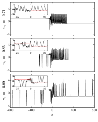
(a) $\xi=0.1$

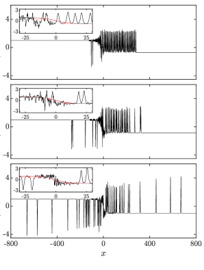
(b) $\xi=10$

Figure 26: Numerical solution at $t=1000$ for narrow (a) and broad (b) smoothed step initial data in the incoherent regime: $u_{+}\lessapprox-0.7$. The insets are zoomed-in and include the initial condition (red).

6.4 Incoherent solitary wavetrain

As the initial smoothed step height is increased through the DSW implosion regime that is described in the previous subsection, a new feature emerges when $-u_{-}<u_{+}<\sigma_{3}(\xi)u_{-}$ (cf. Fig. 1d): the emission of solitary waves. This effect is thoroughly described in section 5 for expansive initial data. We now examine solitary wave emission accompanying compressive data. This subsection is somewhat speculative and brief because we base our description of the dynamics solely upon numerical simulation.

Figure 26 depicts the numerical solution for narrow 26(a) and broad 26(b), smoothed step initial data. In the vicinity of $u_{+}=-0.7$, we observe a depression solitary wave emitted to the left edge of the two-phase oscillatory region II (recall Fig. 25) by $t=1000$. Other simulations, not shown, exhibit solitary wave emission at later times for $u_{+}\approx-0.65$. As the right edge $u_{+}$ is reduced below $-0.7$, more solitary waves, including elevation solitary waves propagating to the right, are emitted. These simulations depict a gradual transition as $u_{+}$ is decreased from DSW implosion to the emission of solitary waves of an increasingly incoherent character. As $u_{+}$ approaches $-u_{-}$, the solitary waves exhibit different amplitudes and are emitted intermittently as shown in the simulation animations that are included as supplementary material to this manuscript. While the simulations for different smoothed step width $\xi$ shown in Figs. 26(a) and 26(b) exhibit differences, their qualitative character is the same. This stands in contrast to the case of solitary wave shedding for expansive data where we showed in section 5 that the initial smoothed step width must be sufficiently narrow, i.e. the initial data must include a sufficiently small scale feature. We remark that qualitatively similar dynamics were observed numerically for broad, localized initial and periodic data in [21].

These pseudospectral simulations were highly resolved. The numerical method is different from that utilized in other sections of the paper (see Appendix A.1) and is described in [11]. The grid spacing $\Delta x=0.00343$ and timestep $\Delta t=0.002$ ensured that the conserved energy $E(t)$ in eq. (5.15) remains numerically within $10^{-10}$ of its predicted value $E(t)=\tfrac{1}{3}(u_{+}^{3}-u_{-}^{3})t+E(0)$ (eq. (5.14)) for the simulated times $t\in[0,1000]$ and domain $x\in[-900,900]$. In all cases, the relative magnitude of the Fourier coefficients $|\hat{u}(k,t)/\hat{u}(0,t)|$ decays to $10^{-15}$ for sufficiently large $k$. Furthermore, the large spatial domain ensures that the boundary deviations from $u_{\pm}$ remain below $10^{-15}$ in magnitude for the simulated times.

One important finding from the simulations in Figure 26 is that even a slight asymmetry in the initial smoothed step ($u_{+}=-0.99u_{-}$) leads to a significant departure from the symmetric dispersive Lax shock that is generated when $u_{+}=-u_{-}$ (recall section 4.1). The animations for this case that are included as supplementary material are particularly revealing in this regard. Thus, the dispersive Lax shock lacks robustness to small changes in the boundary conditions.

7 Conclusions and Outlook

In this paper, we have developed a classification of solutions to the dispersive Riemann problem for the BBM equation. The BBM equation (1.1) as a mathematical model for unidirectional, weakly nonlinear dispersive shallow water wave propagation is asymptotically equivalent to the celebrated KdV equation while providing more satisfactory short-wave/high-frequency behavior in the sense that the linear dispersion relation is bounded for the BBM equation, but unbounded for the KdV equation. However, the bounded dispersion relation is nonconvex, a property that gives rise to a number of intriguing features that are markedly different from those found in the KdV equation. Some of these features exemplify phenomena previously observed in other nonlinear dispersive equations, but some are new, providing the motivation for the study of the reduced BBM equation (1.4) as a distinct dispersive regularization of the Hopf equation.

The main feature of the BBM equation (1.4) that distinguishes it from the KdV equation (1.3) is the non-evolutionary dispersive term $-u_{xxt}$. This term introduces an intrinsic nonlocality length scale $\ell$ and results in a qualitative and quantitative dependence of solutions on the comparison between $\ell$ and the typical spatial scale $\xi$ associated with the initial condition. The nonlocality length $\ell$ coincides with the BBM coherence length (the unit amplitude solitary wave width) defined by the balance of nonlinearity and dispersion. In the normalization of (1.4), $\ell=1$. The nonlocal nature of the BBM equation (1.4) imparts a bounded linear dispersion relation $\omega=\omega_{0}(k,\overline{u})$ that is nonconvex, exhibiting zero-dispersion points $\partial_{kk}\omega_{0}(k,\overline{u})=0$ for particular values of the wavenumber and background. Generally, we find that the complex interplay between nonlocality, nonlinearity and nonconvex dispersion in the BBM equation gives rise to remarkably rich dynamics for the smoothed dispersive Riemann problem with initial data (1.7) in the form of a monotone transition between two constant states $u_{-}$ at $x\to-\infty$ and $u_{+}$ at $x\to+\infty$. We identify regions in the plane of boundary states $(u_{-},u_{+})$ where BBM solutions exhibit qualitatively different behaviors. Additionally, the evolution of data within these regions often depends significantly upon the smoothing of the initial data characterized by its transition width $\xi$, thus introducing a further distinction between various regions. To capture the smoothing-dependent features, we construct two separate dispersive Riemann problem classifications: for $\xi\gg 1$ and for $\xi\ll 1$ shown in Figures 1 and 2, respectively. A detailed guide to the wave patterns presented in these figures is contained in Section 2, which summarizes our findings.

Emergent wave phenomena for the BBM dispersive Riemann problem can be roughly split into two categories: classical and nonclassical. Classical phenomena include dispersive shock waves (DSWs) and rarefaction waves, which are also observed in convex, KdV-type dispersive hydrodynamics, hence termed classical. The nonclassical features are due to nonconvex dispersion and include the generation of two-phase linear wavetrains, expansion shocks, solitary wave shedding, dispersive Lax shocks (in a conservative dispersive equation!), DSW implosion and the generation of incoherent solitary wavetrains. Some of these striking nonclassical features are present only in the evolution of narrow initial steps, $\xi\ll 1$. We stress that all the observed nonclassical phenomena involve short wave features that are formally not applicable in the traditional asymptotic regime of the original BBM equation (1.1) in which $u_{xxt}\sim-u_{xxx}$.

The description of a diverse range of linear and nonlinear wave patterns emerging from the BBM dispersive Riemann problem has required an equally diverse set of approaches—analytical and numerical—to their analysis and description. We analyze linear wavetrains generated near the zero dispersion point using the stationary phase method and matched asymptotics, while solitary wave shedding is tackled by a combination of short time analysis and energy arguments. DSWs in the convex propagation regime, defined by strict hyperbolicity and genuine nonlinearity of the associated Whitham modulation system, are analyzed using the extended DSW fitting method while DSW implosion dynamics are shown to be approximately described by the coupled NLS equation derived from BBM via multiple-scale expansions for weakly nonlinear, two-phase waves. All analytical results are accompanied by detailed numerical simulations. The numerical methods and approaches are presented in the Appendix.

Overall, our analysis shows that the BBM equation describes nonclassical dispersive hydrodynamics that are distinct from previously studied systems with nonconvex flux (modified KdV and Gardner equations [11, 30], Miyata-Choi-Camassa system [19], derivative NLS equation [27]) and higher order/nonconvex dispersion (Kawahara equation [45, 46], nonlocal NLS equation [18, 3]).

Another interpretation of these results incorporates the distinction between long and short waves, evident in the aforementioned difference between the linear dispersion relations for KdV (1.3) and BBM (1.4) in which the phase and group velocities, although asymptotically equivalent for long waves, are bounded for BBM and unbounded for KdV in the short wave regime. While linear theory predicts that short waves in BBM are feeble, in the words of the equation’s namesake [4], nonlinear wave propagation does not suffer from this restriction [37]. The prevalence of nonlinear, short-long wave interaction in the dispersive Riemann problem for BBM is striking. When a short scale is encoded in the initial condition, new features arise in the solution, including expansion shocks, the emission of solitary waves, and 2-phase linear wavepackets. Short wave effects also arise during the course of nonlinear evolution, independent of the spatial scale of the initial data. Dispersive shock wave implosion, the dispersive Lax shock, and incoherent solitary wavetrains are notable examples. In fact, the self-similar dispersive Lax shock $u(x,t)=g(xt)$ exhibits short waves that are unbounded in wavenumber as $t\to\infty$. While a slight asymmetry in the boundary conditions arrests the unbounded wavenumber production in the dispersive Lax shock, the resulting intermittent solitary wave emission suggests a conservative counterpart to the chaos observed in numerical simulations of a damped-driven BBM equation [42]. None of these short wave effects occur in the KdV equation.

Some of the results obtained in this paper carry over to other dispersive hydrodynamic systems. The observed prominent dependence of the long-time dynamics on the initial transition width points to a leading order effect that has mostly been ignored in previous DSW studies. The analysis of two-phase linear wavetrains near a zero dispersion point is general, and the coupled NLS description of DSW implosion can be applied to the conduit and magma equations where this effect is known to occur. Expansion shocks and solitary wave shedding have been observed in the regularized Boussinesq shallow water system [17] albeit in a nonphysical, short-wave regime. Still, it would be fair to say that many of the striking nonconvex wave regimes generated in the BBM dispersive Riemann problem await their realization in other systems.

Our work poses a number of interesting questions that will hopefully be addressed in future research. These include a better understanding of solitary wave shedding and the intermittency associated with the incoherent solitary wave regime, stability analysis of dispersive Lax shocks, and a full analytical description of the nonlinear two-phase structures and envelope solitary waves associated with DSW implosion.

Appendix A Numerical method

A.1 Scheme for the BBM equation

The numerical method described here has been used to solves numerically the Riemann problem (1.4),(1.7). It incorporates a standard fourth-order Runge–Kutta timestepper and a pseudo-spectral Fourier spatial discretization. A different method is used in Sec. 6.4.

The initial condition (1.7) is implemented with the $L$-periodic function:

$$u_{0}^{\rm num.}(x)=\frac{u_{+}-u_{-}}{2}\left(\tanh\left[\frac{x}{\xi}\right]+\tanh\left[\frac{x-L/2}{\xi}\right]\right)+u_{-}.$$ (A.1)

$L$ is sufficiently large such that the hydrodynamic states generated by the steps at $x=0$ and $x=L/2$ do not overlap at time $t$. Note that $L\gg\xi$ and $|u_{0}^{\rm num.}(x)-u_{\pm}|<10^{-15}$ far from the step locations. The grid spacing is $\Delta x\approx 0.0114$.

The spatial Fourier transform of the BBM equation reads:

$$\frac{\mathrm{d}\hat{u}}{\mathrm{d}t}=\frac{-ik}{2(1+k^{2})}\widehat{u^{2}},$$ (A.2)

where $\hat{u}(k,t)$ is the spatial Fourier transform of $u(x,t)$. The truncation of the Fourier domain of $\hat{u}$ turns (A.2) into a nonlinear ordinary differential equation which is temporally evolved according to the fourth-order Runge–Kutta method with a timestep $\Delta t=0.1$. The computation of the Fourier transform of $\widehat{u^{2}}$ is implemented using the fast Fourier transform.

A.2 Determination of the linear wave parameters

We detail in this section the procedure to extract from the numerical solution the wave parameters of the, beating, two-phase wave observed in the region $x<0$ in Sec. 3. In the following the index $i=1$ ($i=2$) denotes the wave with a modulated wavenumber smaller (larger) than $\sqrt{3}$.

We first compute the Fourier transform $\hat{\varphi}(k,t)$ of the numerical solution $\varphi(x,t)=u(x,t)-u_{-}$. $\varphi(x,t)$ is given by:

$$\varphi(x,t)=\frac{1}{2\pi}\int_{\mathbb{R}}\hat{\varphi}(k,t)e^{ikx}dk=\varphi_{1}(x,t)+\varphi_{2}(x,t),$$ (A.3)

where $\varphi_{1}(x,t)=1/2\pi\int_{|k|<\sqrt{3}}\hat{\varphi}(k,t)e^{ikx}dk$ and $\varphi_{2}(x,t)=1/2\pi\int_{|k|>\sqrt{3}}\hat{\varphi}(k,t)e^{ikx}dk$ are, with a good approximation, two distinct one-phase linear waves, cf. Fig. 27. We then extract from the variations of $\varphi_{1}$ and $\varphi_{2}$ the modulated wavenumbers $k_{1}(x,t)$ and $k_{2}(x,t)$. By definition the distinction between $\varphi_{1}$ and $\varphi_{2}$ should only hold in the $(x,t)$-region where $k_{1}(x,t)\ll\sqrt{3}\ll k_{2}(x,t)$. In practice we see in Fig. 3 that the two linear waves are still distinct even if $k_{1}$ and $k_{2}$ are close to $\sqrt{3}$.

Note that we also obtain numerically $k_{1}\sim k_{2}\sim\sqrt{3}$ for $x\ll s_{\rm min}t$ even if no linear waves can propagate in the region. This is a numerical artifact and one can check that $\varphi_{1}$ and $\varphi_{2}$ are out of phase in this region such that $\varphi=\varphi_{1}+\varphi_{2}=0$ as expected.

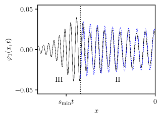
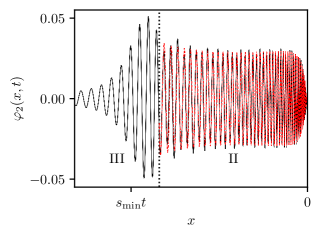
Figure 27: Variation of the linear waves $\varphi_{1}(x,t)$ and $\varphi_{2}(x,t)$ (black solid lines) for the dispersive Riemann problem $(\xi,u_{-},u_{+})=(0.1,1,1.5)$ at $t=500$. For comparison we plot the corresponding stationary phase solution in dashed line: the left (right) plot displays the first (second) term of (A.3). Note that the discrepancy between the analytical solution and the numerical solution and is due to the violation of the small amplitude, cf. discussion in Sec.3.

Appendix B HNLS description

B.1 HNLS equation

The NLS equation displays both a dispersive effect term $A_{xx}\propto\varepsilon^{3}$ and a weakly nonlinear term $|A|^{2}A\propto\varepsilon^{3}$, where $\varepsilon$ is the small parameter describing the slow spatio-temporal dependence and small amplitude of the envelope $A(x,t)$, cf. [5]. The next order of the envelope dynamics of the weakly nonlinear wave:

$$u(x,t)\sim u_{0}+\left[A(x,t)e^{i(\kappa_{0}x-\omega_{0}(\kappa_{0},u_{0})t)}+{\mathrm{c.c.}}\right]+B(x,t),$$ (B.1)

is commonly called higher order NLS (HNLS) equation, includes the terms: $A_{xxx}\propto\varepsilon^{4}$, $|A|^{2}A_{x}\propto\varepsilon^{4}$ and $A^{2}A^{*}_{x}\propto\varepsilon^{4}$ (cf. our paper and references therein). The HNLS equation for the BBM equation reads:

$$\begin{split}&iA_{t}+i\partial_{k}\omega_{0}A_{x}+\beta A_{xx}+\gamma|A|^{2}A+i\delta A_{xxx}+i\lambda|A|^{2}A_{x}+i\nu A^{2}A^{*}_{x}=0,\\ &B=b|A|^{2}+\frac{i}{2}b_{2}(AA^{*}_{x}-A^{*}A_{x})=b\frac{a^{2}}{16}+b_{2}\frac{a^{2}v}{16}.,\end{split}$$ (B.2)

where the coefficients $\beta$, $\gamma$ and $b$ are given in (6.31), and $a$ and $v$ are defined in (6.11). $\delta$, $\lambda$, $\nu$ and $b_{2}$ are function of the parameters $\kappa_{0},u_{0}$ given by:

$$\begin{split}&\delta=\frac{u_{0}(1-6\kappa_{0}^{2}+\kappa_{0}^{4})}{(1+\kappa_{0}^{2})^{4}},\;\lambda=\frac{-9-9\kappa_{0}^{2}+9\kappa_{0}^{4}+5\kappa_{0}^{6}}{3u_{0}(3+\kappa_{0}^{2})^{2}(\kappa_{0}^{2}+\kappa_{0}^{4})},\;\\ &\nu=\frac{-27-21\kappa_{0}^{2}+19\kappa_{0}^{4}+5\kappa_{0}^{6}}{6u_{0}(3+\kappa_{0}^{2})^{2}(\kappa_{0}^{2}+\kappa_{0}^{4})},\;b_{2}=\frac{-2(\kappa_{0}^{2}-3)(1+\kappa_{0}^{2})}{u_{0}\kappa_{0}^{3}(3+\kappa_{0}^{2})^{2}}.\end{split}$$ (B.3)

B.2 DSW modulation

The universal DSW modulation near the trailing edge is given by the following special self-similar rarefaction wave solution of (B.2), cf. [10]:

$$\begin{split}&\lambda_{-}\frac{a^{2}}{16}+2\beta_{-}v-3\delta_{-}v^{2}-{\rm sgn}(\beta_{-})\frac{a^{2}}{16}\sqrt{D(a,v)}=\frac{x}{t}-s_{-},\\ &D(a,v)=\nu_{-}^{2}-\frac{32(\beta_{-}-3\delta_{-}v)(\gamma_{-}-(\lambda_{-}-\nu_{-})v)}{a^{2}},\end{split}$$ (B.4)

where $a$ and $v$ are related by the differential equation:

$$\frac{\mathrm{d}v}{\mathrm{d}a}+\frac{\nu_{-}+{\rm sgn}(\beta_{-})a\sqrt{D(a,v)}}{16(\beta_{-}-3\delta_{-}v)},\quad v(0)=0.$$ (B.5)

The parameters $\beta_{-}$, $\gamma_{-}$, $\delta_{-}$, $\lambda_{-}$ and $\nu_{-}$ are the coefficients $\beta$, $\gamma$, $\delta$, $\lambda$ and $\nu$ evaluated at $(\kappa_{0},u_{0})=(k_{-},u_{-})$ where $k_{-}$ is given by (6.18).

Appendix C Stability of nonlinear two-phase solution

In [23], it was shown that the stability of the plane wave solution (6.50) to the coupled NLS equations (6.45) boils down to determining the roots $v$ of the quartic polynomial

$$\begin{split}&\left((v-v_{g1})^{2}+Q_{1}(q)\right)\left((v-v_{g2})^{2}+Q_{2}(q)\right)-R=0,\\ &Q_{j}(q)=-\beta_{j}^{2}q^{2}+\frac{1}{8}a_{j}^{2}\beta_{j}\gamma_{j},\quad R=\frac{1}{64}\beta_{1}\beta_{2}\nu_{12}\nu_{21}a_{1}^{2}a_{2}^{2},\end{split}$$ (C.1)

where we have introduced the notation $v_{gj}=\partial_{k}\omega_{0}(\kappa_{j},u_{-})$, $\beta_{j}\equiv\beta(\kappa_{j},u_{-})$, $\gamma_{j}\equiv\gamma(\kappa_{j},u_{-})$, and $\nu_{ij}\equiv\nu(\kappa_{i},\kappa_{j},u_{-})$ for brevity. A root $v$ of the quartic (C.1) is the phase velocity and $q$ is the wavenumber, both of the infinitesimal plane wave perturbation $\propto\exp(iq(x-vt))$ of the nonlinear solution (6.50). Consequently, if all four roots of (C.1) are real for every $q\in\mathbb{R}$, then the weakly nonlinear two-phase wavetrain (6.50) is modulationally stable.

In general, there are no simple, explicit expressions for the roots of (C.1). However, a simplification of the general calculations in [23] can be made when the two group velocities $v_{g1}$, $v_{g2}$ are close so that (C.1) can be approximated by taking $(v-v_{gj})^{2}\to(v-\bar{v}_{g})^{2}$ where $\bar{v}_{g}=\frac{1}{2}(v_{g1}+v_{g2})$ is the average of the group velocities. Then $(v-\bar{v}_{g})^{2}$ in the approximation of (C.1) satisfies a quadratic equation. Introducing the difference of the group velocities $\Delta v_{g}=\frac{1}{2}(v_{g2}-v_{g1})$ and assuming $|\Delta v_{g}/\bar{v}_{g}|\ll 1$, the four roots of (C.1) are approximately

$$2(v-\bar{v}_{g}\pm\Delta v_{g})^{2}=-Q_{1}(q)-Q_{2}(q)\pm\sqrt{(Q_{2}(q)-Q_{1}(q))^{2}+4R}.$$ (C.2)

Then the necessary and sufficient condition for stability is the real, non-negativity of $-Q_{1}(q)-Q_{2}(q)\pm\sqrt{(Q_{2}(q)-Q_{1}(q))^{2}+4R}$. Since $Q_{1}(q)<0$ and $Q_{2}^{\prime}(q)<0$, it suffices to consider only the long wavelength case $q=0$. For the simulation shown in Fig. 23, we calculate

$$-Q_{1}(0)-Q_{2}(0)\pm\sqrt{(Q_{2}(0)-Q_{1}(0))^{2}+4R}\approx 0.0111\pm 0.0109>0,$$ (C.3)

hence the two-phase plane wave solution (6.50) is stable. A plot of the linear dispersion relation $v=v(q)$ for perturbations to (6.50) as roots of (C.1) and their approximation (C.2) for the extracted simulation parameters in Fig. 23 is shown in Fig. 28.

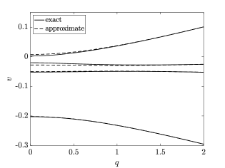
Figure 28: Linear dispersion relation $v(q)$ for perturbations to the plane wave solution (6.50) corresponding to Fig. 23. The exact roots of (C.1) (solid) and their approximation (C.2) (dashed) are shown. All are purely real, implying modulational stability of region IIa.

References

- [1] Mark J. Ablowitz and Douglas E. Baldwin. Dispersive shock wave interactions and asymptotics. Physical Review E, 87(2), 2013.
- [2] M. Abramowitz and I. A. Stegun, editors. Handbook of mathematical functions: with formulas, graphs, and mathematical tables. Dover books on mathematics. Dover Publ, New York, NY, 9. dover print edition, 2013.
- [3] Saleh Baqer and Noel F. Smyth. Modulation theory and resonant regimes for dispersive shock waves in nematic liquid crystals. Physica D: Nonlinear Phenomena, 403:132334, 2020.
- [4] T. B. Benjamin, J. L. Bona, and J. J. Mahony. Model equations for long waves in nonlinear dispersive systems. Philos. Trans. Royal Soc. A, 272(1220):47–78, March 1972.
- [5] D. J. Benney and A. C. Newell. The Propagation of Nonlinear Wave Envelopes. Journal of Mathematics and Physics, 46(1-4):133–139, April 1967.
- [6] Deniz Bilman and Thomas Trogdon. On numerical inverse scattering for the Korteweg–de Vries equation with discontinuous step-like data. Nonlinearity, 33(5):2211–2269, 2020.
- [7] Gino Biondini and Thomas Trogdon. Gibbs phenomenon for dispersive PDEs on the line. SIAM J. Appl. Math., 77(3):813–837, 2017.
- [8] C. Chester, B. Friedman, and F. Ursell. An extension of the method of steepest descents. Proc. Comb. Phil. Soc., 53(3):599–611, July 1957. Publisher: Cambridge University Press.
- [9] M. S. Child. Semiclassical Mechanics with Molecular Applications. Oxford University Press, 2 edition, 2014.
- [10] T. Congy, G. A. El, M. A. Hoefer, and M. Shearer. Nonlinear Schrödinger equations and the universal description of dispersive shock wave structure. Stud. Appl. Math, 142(3):241–268, April 2019.
- [11] G. El, M. Hoefer, and M. Shearer. Dispersive and diffusive-dispersive shock waves for nonconvex conservation laws. SIAM Review, 59:3–61, 2017.
- [12] G. A. El. Resolution of a shock in hyperbolic systems modified by weak dispersion. Chaos, 15(3):037103, September 2005.
- [13] G. A. El, R. H. J. Grimshaw, and N. F. Smyth. Transcritical shallow-water flow past topography: finite-amplitude theory. Journal of Fluid Mechanics, 640(1):187–214, 2009.
- [14] G. A. El, R. H. J. Grimshaw, and N.F. Smyth. Asymptotic description of solitary wave trains in fully nonlinear shallow-water theory. Physica D, 237(19):2423–2435, 2008.
- [15] G. A. El, M. A. Hoefer, and M. Shearer. Expansion shock waves in regularized shallow-water theory. Proc. R. Soc. A, 472(2189):20160141, May 2016.
- [16] G.A. El and M.A. Hoefer. Dispersive shock waves and modulation theory. Physica D: Nonlinear Phenomena, 333:11–65, October 2016.
- [17] Gennady A. El, Mark A. Hoefer, and Michael Shearer. Stationary Expansion Shocks for a Regularized Boussinesq System. Studies in Applied Mathematics, 140(1):27–47, 2018.
- [18] Gennady A. El and Noel F. Smyth. Radiating dispersive shock waves in non-local optical media. Proceedings of the Royal Society A: Mathematical, Physical and Engineering Science, 472(2187):20150633, March 2016.
- [19] J. G. Esler and J. D. Pearce. Dispersive dam-break and lock-exchange flows in a two-layer fluid. Journal of Fluid Mechanics, 667:555–585, 2011.
- [20] H. Flaschka, M. G. Forest, and D. W. McLaughlin. Multiphase averaging and the inverse spectral solution of the Korteweg-de Vries equation. Comm. Pure Appl. Math., 33:739–784, 1980.
- [21] M. Francius, E. Pelinovsky, and A. Slunyaev. Wave dynamics in nonlinear media with two dispersionless limits for long and short waves. Physics Letters A, 280(1-2):53–57, 2001.
- [22] T Grava and C Klein. Numerical study of a multiscale expansion of the Korteweg–de Vries equation and Painlevé-II equation. Proc. Roy. Soc. A, 464(2091):733–757, 2008.
- [23] S. D. Griffiths, R. H. J. Grimshaw, and K. R. Khusnutdinova. Modulational instability of two pairs of counter-propagating waves and energy exchange in a two-component system. Physica D: Nonlinear Phenomena, 214(1):1–24, 2006.
- [24] R. H. J. Grimshaw and N. F. Smyth. Resonant flow of a stratified fluid over topography. J. Fluid Mech, 169:429–464, 1986.
- [25] A. V. Gurevich and L. P. Pitaevskii. Nonstationary structure of a collisionless shock wave. Sov. Phys. JETP, 38(2):291–297, 1974. Translation from Russian of A. V. Gurevich and L. P. Pitaevskii, Zh. Eksp. Teor. Fiz. 65, 590-604 (August 1973).
- [26] M. A. Hoefer. Shock Waves in Dispersive Eulerian Fluids. Journal of Nonlinear Science, 24(3):525–577, 2014.
- [27] S. K. Ivanov and A. M. Kamchatnov. Riemann problem for the photon fluid: Self-steepening effects. Physical Review A, 96(5):053844, 2017.
- [28] A. M Kamchatnov. Nonlinear periodic waves and their modulations: an introductory course. World Scientific, 2000.
- [29] A. M. Kamchatnov. Dispersive shock wave theory for nonintegrable equations. Physical Review E, 99(1), January 2019.
- [30] A. M. Kamchatnov, Y.-H. Kuo, T.-C. Lin, T.-L. Horng, S.-C. Gou, R. Clift, G. A. El, and R. H. J. Grimshaw. Undular bore theory for the Gardner equation. Physical Review E, 86(3):036605, 2012.
- [31] P. D. Lax. Hyperbolic systems of conservation laws II. Commun. Pure Appl. Math., 10(4):537–566, 1957.
- [32] P. D. Lax. Hyperbolic systems of conservation laws and the mathematical theory of shock waves. SIAM, 1973.
- [33] J A Leach and D J Needham. The large-time development of the solution to an initial-value problem for the Korteweg–de Vries equation: I. Initial data has a discontinuous expansive step. Nonlinearity, 21(10):2391–2408, 2008.
- [34] N. K. Lowman and M. A. Hoefer. Dispersive hydrodynamics in viscous fluid conduits. Physical Review E, 88(2):023016, 2013.
- [35] Nicholas K. Lowman and M. A. Hoefer. Dispersive shock waves in viscously deformable media. Journal of Fluid Mechanics, 718:524–557, 2013.
- [36] M. D. Maiden, N. A. Franco, E. G. Webb, G. A. El, and M. A. Hoefer. Solitary wave fission of a large disturbance in a viscous fluid conduit. Journal of Fluid Mechanics, 883:A10, January 2020.
- [37] M. A. Manna and V. Merle. Asymptotic dynamics of short waves in nonlinear dispersive models. Phys. Rev. E, 57(5):6206–6209, 1998.
- [38] T. R. Marchant and N. F. Smyth. Initial-boundary value problems for the Korteweg-de Vries equation. IMA J. Appl. Math, 47(3):247–264, 1991.
- [39] Peter Olson and Ulrich Christensen. Solitary Wave Propagation in a Fluid Conduit Within a Viscous Matrix. Journal of Geophysical Research, 91(B6):6367–6374, 1986.
- [40] P. J. Olver. Euler operators and conservation laws of the BBM equation. Math. Proc. Camb. Philos. Soc., 85(1):143–160, January 1979.
- [41] D. H. Peregrine. Calculations of the development of an undular bore. J. Fluid Mech, 25(2):321–330, 1966.
- [42] Erico L. Rempel and Abraham C.-L. Chian. Origin of transient and intermittent dynamics in spatiotemporal chaotic systems. Phys. Rev. Lett., 98(1):014101, 2007.
- [43] David R. Scott and David J. Stevenson. Magma solitons. Geophysical Research Letters, 11(11):1161–1164, 1984.
- [44] N. F. Smyth. Modulation theory solution for resonant flow over topography. Proc. Roy. Soc. Ser. A, 409(1836):79–97, 1987.
- [45] P. Sprenger and M. Hoefer. Shock Waves in Dispersive Hydrodynamics with Nonconvex Dispersion. SIAM Journal on Applied Mathematics, 77:26–50, 2017.
- [46] Patrick Sprenger and Mark A Hoefer. Discontinuous shock solutions of the Whitham modulation equations as zero dispersion limits of traveling waves. Nonlinearity, 33(7):3268–3302, 2020.
- [47] Aaron G. Stubblefield, Marc Spiegelman, and Timothy T. Creyts. Solitary waves in power-law deformable conduits with laminar or turbulent fluid flow. Journal of Fluid Mechanics, 886:A10, 2020.
- [48] J. A. Whitehead and K. R. Helfrich. Magma waves and diapiric dynamics. In M. P. Ryan, editor, Magma Transport and Storage, pages 53–76. John Wiley & Sons, Chichester, UK, 1990.
- [49] A. J. Whitfield and E. R. Johnson. Wave-packet formation at the zero-dispersion point in the Gardner-Ostrovsky equation. Phys. Rev. E, 91(5), 2015.
- [50] G. B. Whitham. Non-linear dispersive waves. Proc. Roy. Soc. Ser. A, 283:238–261, 1965.
- [51] G. B. Whitham. Linear and nonlinear waves. Pure and applied mathematics. Wiley, New York, NY, 2 edition, 1999. OCLC: 246124655.