Gradient Descent Averaging and Primal-dual Averaging
for Strongly Convex Optimization

Abstract

Averaging scheme has attracted extensive attention in deep learning as well as traditional machine learning. It achieves theoretically optimal convergence and also improves the empirical model performance. However, there is still a lack of sufficient convergence analysis for strongly convex optimization. Typically, the convergence about the last iterate of gradient descent methods, which is referred to as individual convergence, fails to attain its optimality due to the existence of logarithmic factor. In order to remove this factor, we first develop gradient descent averaging (GDA), which is a general projection-based dual averaging algorithm in the strongly convex setting. We further present primal-dual averaging for strongly convex cases (SC-PDA), where primal and dual averaging schemes are simultaneously utilized. We prove that GDA yields the optimal convergence rate in terms of output averaging, while SC-PDA derives the optimal individual convergence. Several experiments on SVMs and deep learning models validate the correctness of theoretical analysis and effectiveness of algorithms.

Introduction

Averaging scheme has been widely adopted from different angles. It always helps to reduce variance and improve generalization of learning algorithms. In fact, there exist various averaging techniques, such as dual averaging (DA) (Nesterov 2009), weight averaging (WA) (Izmailov et al. 2018), output averaging (OA) (Nemirovsky and Yudin 1983; Polyak and Juditsky 1992), primal averaging (PA) (Nesterov and Shikhman 2015; Tao et al. 2020), etc.

DA was initially proposed by Nesterov (Nesterov 2009), which averages all past gradient information at each iteration. In comparison with gradient descent (GD) and mirror descent (MD) (Beck and Teboulle 2003), it avoids new gradients to be considered with less weight than previous ones (Flammarion and Bach 2017). DA has been successfully extended to the stochastic composite scenario and it’s well-suited for large-scale learning problems (Xiao 2009; Dekel et al. 2012). The superiority of regularized dual averaging (RDA) in efficiently promoting regularizer structure (e.g., sparsity) has been elaborated by Xiao and also earned test of time award at NeurIPS (Xiao 2009).

Recently, averaging has also been frequently employed in training deep neural networks. WA averages weights of the networks based on training epochs (Izmailov et al. 2018). Since then, a series of contribution: SWALP (Yang et al. 2019), Fast-SWA (Athiwaratkun et al. 2018), SWA-Guassian (Maddox et al. 2019) have been successfully applied to a wide range of applications. Besides, exponential moving average (EMA), which has been used to exponentially decay the weights for previous iterate, can be regarded as a particular example of WA (Kingma and Ba 2014; Reddi, Kale, and Kumar 2019; Ma and Yarats 2018).

OA is a classical way about how to output the final solution for iterative algorithms. Existing convergence analyses mostly center on it due to some superior theoretical guarantees (Dimitri P., Angelia., and Asuman E. 2003). Actually, running algorithms for $t$ iterations, and returning the last iterate, is a very intuitive idea in practice. Therefore, there are still some gaps about individual output between theoretical analyses and practical implementations. Several works on stochastic gradient descent (SGD) develop different OA techniques to achieve the optimal convergence rate, especially for strongly convex optimization, such as suffix averaging (Rakhlin, Shamir, and Sridharan 2011), non-uniform averaging (Lacoste-Julien, Schmidt, and Bach 2012; Harvey, Liaw, and Randhawa 2019), increasing weighted averaging (Guo et al. 2020), etc.

The optimal convergence for strongly convex problems has become a challenging problem after the well-known work (Hazan et al. 2006). This is because conventional SGD cannot attain the optimal convergence even when we take the uniform average of all past iterates. An open question early posed by (Shamir 2012) is that whether OA is needed at all to attain optimal convergence rate. Partially addressing this question, Shamir et al. (Shamir and Zhang 2013) showed that SGD with polynomial-decay averaging has an $O({\log t}/{\sqrt{t}})$ individual convergence rate in the general strongly convex cases and an $O({\log t}/{t})$ rate in strongly convex cases, respectively. Recent works (Harvey et al. 2019; Jain, Nagaraj, and Netrapalli 2019) provide the affirmative answer that the logarithmic term in the convergence bound is necessary for any plain SGD in both general convex and strongly convex cases. However, they leave us a new challenging problem. Can we achieve the optimal rate of $O(1/t)$ by slightly modifying any classical algorithms? From these observations, there are mainly two ways to achieve the optimal rate without the logarithmic factor. One is to modify the original steps of the algorithms. The other is to employ the averaging strategy.

PA is an interesting gradient operation step, in which the gradient evaluation is imposed on the weighted average of all past iterative solutions (Tao et al. 2020). In fact, this averaging scheme was first used in PDA (Nesterov and Shikhman 2015), which exploits simultaneously in both primal and dual space per-iteration, and succeeds in deriving the optimal individual rate for minimizing non-smooth general convex objectives. Later, (Tao et al. 2020) formally named it as PA, and they focus on projected subgradient (PSG) method. Its individual convergence rate doesn’t suffer from the extra logarithmic factor. Overall, PDA is the closest solution to eliminate the $\log t$ factor about DA. Unfortunately, (Nesterov and Shikhman 2015) partially addressed the optimal convergence problem only in the general convex scenario. Optimal-RDA (Chen, Lin, and Pena 2012) proposed earlier than PDA, requires two gradient operations per-iteration, which is different from conventional DA with only one operation. Similarly, (Cutkosky 2019) and (Joulani et al. 2020) add an auxiliary PA scheme into their algorithms, which are able to achieve the optimal regret bound in the online setting.

This paper is motivated by the breakthrough work of (Nesterov and Shikhman 2015). Our original intention is to derive the optimal individual convergence of DA with minor changes in gradient operations. The main contributions can be summarized as follows:

• We present a general GDA algorithm, which includes the strongly convex algorithm in (Cutkosky 2019) as one special case of our method. Our GDA gains a deeper insight into the connection between DA and GD. Moreover, we prove that this algorithm no longer suffers from the logarithmic factor and attains the optimal convergence rate $O({1}/{t})$ coupled with OA.

• We incorporate PA into GDA, and develop a novel SC-PDA algorithm so as to achieve optimal individual convergence rate $O({1}/{t})$. Moreover, our convergence analysis of SC-PDA is obviously different from Nesterov’s PDA. Thus, our work theoretically completes the task about individual convergence of DA under different convexity situations.

Preliminaries and Notations

Many convex optimization algorithms in machine learning can be formulated as a constrained black-box problem:

$$\min f(\mathbf{w}),\ s.t.\ \mathbf{w}\in\mathbf{Q}.$$ (1)

where $\mathbf{Q}$ is a bounded convex domain, and $f\left(\cdot\right)$ is a convex function on $\mathbf{Q}$. Denote that $\mathbf{w}_{*}$ is an optimal solution. We use $\nabla f(\mathbf{w})$ to denote the (sub)gradient of $f$ at $\mathbf{w}$ and $\hat{\mathbf{g}}$ is an unbiased estimate of (sub)gradient of $f$ at $\mathbf{w}$.

Following (Shamir and Zhang 2013), we first provide the definitions of strong convexity, individual convergence, and averaged convergence.

Definition 1. A function $f$ is called $\mu$-strongly convex with respect to the norm $\|\cdot\|$ if there is a constant $\mu>0$ such that

$$f(\mathbf{w})\geq f(\mathbf{u})+\langle\nabla f(\mathbf{u}),\mathbf{w}-\mathbf{u}\rangle+\dfrac{\mu}{2}\|\mathbf{w}-\mathbf{u}\|^{2},$$ (2)

for all $\mathbf{u},\mathbf{w}$.

Note that the strong convexity parameter $\mu$ is a measure of the curvature of $f$, $\left<\cdot,\cdot\right>$ stands for the Euclidean inner product, and the quadratic lower bound in (2) can be also satisfied with $\mu=0$ for a convex function.

Generally, the convergence about the last iterate is often referred to as individual convergence for simplicity (Tao et al. 2020).

Definition 2. Given a convex function $f$, let $\{\mathbf{w}_{t}\}_{t>0}$ be generated by optimization algorithms, the individual convergence is defined as

$$f(\mathbf{w}_{t})-f(\mathbf{w}_{*})\leq\epsilon(t).$$ (3)

Definition 3. Given a convex function $f$ with uniform averaged output $\mathbf{\bar{w}}_{t}=\frac{1}{t}\sum_{i=1}^{t}\mathbf{w}_{i}$, let $\mathbf{w}_{t}$ be generated by optimization algorithms, we can define averaged convergence as

$$f(\mathbf{\bar{w}}_{t})-f(\mathbf{w}_{*})\leq\epsilon(t).$$ (4)

The convergence bound $\epsilon$ is related to $t$. In particular, the optimal bound is $O({1}/{\sqrt{t}})$ in the non-smooth convex cases and $O({1}/{t})$ in the strongly convex cases, respectively (Nesterov 1983; Nemirovsky and Yudin 1983).

Related Work

In this section, we briefly review some related algorithms and their convergence rates. PSG is one of the most fundamental algorithms for solving (1), and the iteration of which is,

$$\mathbf{w}_{t+1}=P[\mathbf{w}_{t}-a_{t}\nabla f(\mathbf{w}_{t})],$$ (5)

where $P$ is the projection operator on $\mathbf{Q}$, $a_{t}>0$ is the step-size parameter. More generally, mirror descent (MD) is a direct extension of the PSG by using a mirror map, and it iterates as follows,

$${\mathbf{w}}_{t+1}=\arg\min_{\mathbf{w}\in\mathbf{Q}}\{a_{t}\langle\nabla f(\mathbf{w}_{t}),\mathbf{w}\rangle+B(\mathbf{w},\mathbf{w}_{t})\},$$ (6)

where $t>0$, $B$ is the Bregman divergence. MD recovers PSG by taking $\frac{1}{2}\|\mathbf{w}-\mathbf{w}_{t}\|^{2}$.

Based on MD, DA is also a powerful first-order gradient algorithm (Nesterov 2009). The standard DA updates the solution according to

$${\mathbf{w}}_{t+1}=\arg\min_{\mathbf{w}\in\mathbf{Q}}\{\sum_{k=0}^{t}\langle a_{k}\nabla f(\mathbf{w}_{k}),\mathbf{w}\rangle+\gamma_{t}d(\mathbf{w})\},$$ (7)

where $a_{t}$ is the weight parameter, $\gamma_{t}>0$ is the stepsize, $d(\cdot)$ is a strongly convex function such that

$$d(\mathbf{w})\geq d(\mathbf{u})+\langle\nabla d(\mathbf{u}),\mathbf{w}-\mathbf{u}\rangle+\frac{1}{2}\|\mathbf{w-u}\|^{2},\forall\mathbf{u},\mathbf{w}\in\mathbb{R}^{n}.$$

It has been shown in (Nesterov and Shikhman 2015) that,

$$\frac{1}{A_{t}} \sum_{k=0}^{t}a_{k}f(\mathbf{w}_{k})-f(\mathbf{w}_{*})$$ (8)

$$\leq\frac{1}{A_{t}}\big{[}\gamma_{t}d(\mathbf{w}_{*})+\sum_{k=0}^{t}\frac{a_{k}^{2}}{2\gamma_{k}}\|\nabla f(\mathbf{w}_{k})\|^{2}\big{]}.$$

where $A_{t}=\sum_{k=0}^{t}a_{k}$.

RDA is a proximal variant of DA algorithm that dramatically captures the geometry structure of the regularizer for stochastic composite learning problems. The key iteration is as follows,

$$\mathbf{w}_{t+1}=\arg\min_{\mathbf{w}\in\mathbf{Q}}\{\frac{1}{t}\langle\sum_{k=0}^{t}\nabla f(\mathbf{w}_{k}),\mathbf{w}\rangle+r(\mathbf{w})+\frac{\beta_{t}}{t}d(\mathbf{w})\},$$ (9)

where $r(\mathbf{w})$ is the regularization function, $d(\mathbf{w})$ is a strongly convex regularization term, $\{\beta_{t}\}_{t>0}$ is a non-negative and non-decreasing sequence. RDA (9) accumulates the weight of a sparse regularizer such as $l_{1}$-norm to produce more sparse solutions. By averaging all past gradient instead of using current gradient information, DA always exhibits more stable convergence behavior. Besides, it uses a global proximal function $d(\mathbf{w})$ as opposed to local Bregman divergence $B(\mathbf{w},\mathbf{w}_{t})$ in (6).

In order to obtain the optimal individual convergence rate, (Nesterov and Shikhman 2015) developed PDA where the primal and dual averaging schemes are simultaneously employed. It can be viewed as an alternative answer to the Shamir’s open problem by slightly modifying DA. The key steps can be described as follows,

$$\mathbf{w}_{t}^{+}=\arg\min_{\mathbf{w}\in\mathbf{Q}}\{\sum_{k=0}^{t}\langle a_{k}\nabla f(\mathbf{w}_{k}),\mathbf{w}\rangle+\gamma_{t}d(\mathbf{w})\},$$ (10a)

$$\mathbf{w}_{t+1}=\frac{A_{t}}{A_{t+1}}\mathbf{w}_{t}+\frac{a_{t+1}}{A_{t+1}}\mathbf{w}_{t}^{+}.$$ (10b)

Obviously, the only difference between standard DA (7) and PDA (10) lies in the additional weighted averaging step (10b), also called PA (Tao et al. 2020; Taylor and Bach 2019). Only considering the general convex case, it was proved to derived the optimal individual convergence,

$$f(\mathbf{w}_{t})-f(\mathbf{w}_{*})\leq\frac{1}{A_{t}}[\gamma_{t}d(\mathbf{w}_{*})+\sum_{k=0}^{t}\frac{a_{k}^{2}}{2\gamma_{k}}\|\nabla f(\mathbf{w}_{k})\|^{2}].$$ (11)

Based on the PDA, (Tao et al. 2020) presented PA-PSG for both general convex (12) and strongly convex scenarios (13), such that

$$\mathbf{w}_{t}^{+}=P[\mathbf{w}_{t-1}^{+}-a_{t}\nabla f(\mathbf{w}_{t})],$$ (12a)

$$\mathbf{w}_{t+1}=\frac{A_{t}}{A_{t+1}}\mathbf{w}_{t}+\frac{a_{t+1}}{A_{t+1}}\mathbf{w}_{t}^{+},$$ (12b)

and

$$\mathbf{w}_{t}^{+}=P[\delta_{t}\mathbf{w}_{t-1}^{+}-{a_{t}}{\delta_{t}}(\nabla f(\mathbf{w}_{t})-\mu\mathbf{w}_{t})],$$ (13a)

$$\mathbf{w}_{t+1}=\frac{A_{t}}{A_{t+1}}\mathbf{w}_{t}+\frac{a_{t+1}}{A_{t+1}}\mathbf{w}_{t}^{+},$$ (13b)

where $\delta_{t}=1/(1+a_{t}\mu)$.

Note that the gradient operations are imposed on $f(\mathbf{w}_{t})$, and now $\mathbf{w}_{t}$ becomes a weighted average of all past iterative primal sequences. PA-PSG also achieves the following convergence rate,

$$f(\mathbf{w}_{t})-f(\mathbf{w}_{*})\leq\frac{1}{A_{t}}[B(\mathbf{w}_{0},\mathbf{w}_{*})+\sum_{k=0}^{t}\frac{a_{k}^{2}}{2}\|\nabla f(\mathbf{w}_{k})\|^{2}].$$ (14)

It reveals that PA-PSG in the convex setting converges to the optimum at $O({1}/{\sqrt{t}})$ (Tao et al. 2020). Besides, (Defazio and Gower 2020) also established connections between PA and momentum methods.

Online-to-batch conversion is a standard way to obtain convergence guarantees from online learning algorithms to stochastic convex optimization (Shalev-Shwartz, Singer, and Srebro 2007; Hazan and Kale 2011). Recently, (Cutkosky 2019) developed anytime online learning algorithms whose last iterate converge to the optimum in the stochastic cases. (Cutkosky 2019) focused on DA, and the strongly convex algorithm can be described as follows,

$$\mathbf{w}_{t+1}=\arg\min_{\mathbf{w}\in\mathbf{Q}}\{\langle\sum_{k=0}^{t}\nabla f(\mathbf{w}_{k}),\mathbf{w}\rangle+\frac{\mu}{2}\sum_{k=0}^{t}\|\mathbf{w}-\mathbf{w}_{k}\|^{2}\}.$$ (15)

It has also been proved that

$$\mathbb{E}[f(\mathbf{w}_{t})-f(\mathbf{w})]\leq O\left(\frac{\log t}{2\mu t}\right).$$ (16)

Obviously, this convergence bound (16) for stochastic optimization is suboptimal.

Based on the above observations, we can find that the optimal individual convergence rate of DA for strongly convex optimization problem is still missing, which is one of our main motivations in this paper.

Proposed GDA and SC-PDA Algorithms

In this section, we focus on the case where $f$ satisfies $\mu$-strongly convex, and present two modified projection-based DA algorithms for solving (1), then we will analyse their performance in terms of optimal convergence rate. The proofs of theoretical results in this section are exhibited in the supplementary material.

GDA and Averaged Convergence

Following the work of RDA for strongly convex functions (Xiao 2009), we replace the term $\gamma_{t}d(\mathbf{w})$ in standard DA (7) with another $\mu$-strongly convex term $\frac{\mu}{2}\sum_{k=0}^{t}\gamma_{k}\|\mathbf{w}-\mathbf{w}_{k}\|^{2}$, then we have

$$\mathbf{w}_{t+1}=\arg\min_{\mathbf{w}\in\mathbf{Q}}\{\sum_{k=0}^{t} \langle a_{k}\nabla f(\mathbf{w}_{k}),\mathbf{w}\rangle$$ (17)

$$+\dfrac{\mu}{2}\sum_{k=0}^{t}\gamma_{k}\|\mathbf{w}-\mathbf{w}_{k}\|^{2}\}.$$

We can find that the strongly convex algorithm (15) is one special case of our GDA algorithm (17) when we let $a_{k}=1$ and $\gamma_{k}=1$.

The detailed steps of GDA algorithm are shown in Algorithm 1. According to the following lemmas, we can also get the projection version of DA. We first provide the property of projection operator,

Lemma 1. (Dimitri P., Angelia., and Asuman E. 2003) For $\mathbf{w}\in\mathbb{R}^{n},\mathbf{w}_{0}\in\mathbf{Q}$,

$$\langle\mathbf{w}-\mathbf{w}_{0},\mathbf{u}-\mathbf{w}_{0}\rangle\leq 0,$$

for all $\mathbf{u}\in\mathbf{Q}$ if $\mathbf{w}_{0}=P(\mathbf{w})$.

In the following lemma, we can get the equivalent form between the projection method and the proximal method.

Lemma 2. For $\mathbf{w}\in\mathbb{R}^{n}$, standard DA algorithm (7) is equivalent to

$$\mathbf{w}_{t+1}=P\big{[}-\frac{\sum_{k=0}^{t}a_{k}\nabla f(\mathbf{w}_{k})}{\gamma_{t}}\big{]},$$ (18)

where $P$ is the projection operator on $\mathbf{Q}$.

Based on Lemma 1, we can get the following projection-based DA for strongly convex objectives, which is also equivalent to (17), i.e.,

$$\mathbf{w}_{t+1}=P\big{\{}\frac{1}{\Gamma_{t}}\sum_{k=0}^{t}\gamma_{k}[\mathbf{w}_{k}-\frac{a_{k}}{\mu\gamma_{k}}\nabla f(\mathbf{w}_{k})]\big{\}},$$ (19)

where $t>0$, $\Gamma_{t}=\sum_{k=0}^{t}\gamma_{k}$. The stepsize is ${a_{k}}/(\mu\gamma_{k})$. Notably, this algorithm (19) can be viewed as a weighted averaging GD, which we name GDA in the paper. In contrast to PIWA (Guo et al. 2020), our original intention is to slightly modify DA, and then we build the connection between DA and GD. Besides, PA is different from the weighted averaging scheme employed in PIWA.

Algorithm 1 GDA

0:  strongly convex parameter $\mu$, non-negative stepsize sequence $a_{t}$ and $\gamma_{t}$.

1:  Initialize $\mathbf{w}_{0}=\mathbf{0}$, $a_{0}=0,\gamma_{0}=\Gamma_{0}=0$.

2:  repeat

3:     Calculate $\Gamma_{t+1}=\Gamma_{t}+\gamma_{t+1}$,

4:     Compute subgradient of $\nabla f(\mathbf{w}_{t})$,

5:     Update (sub)gradient descent step:$\mathbf{w}_{t1}=\mathbf{w}_{t}-\frac{a_{t}}{\gamma_{t}\mu}\nabla f(\mathbf{w}_{t})$,

6:     Update weighted averaging step:$\mathbf{w}_{t2}=\frac{1}{\Gamma_{t}}\sum_{k=0}^{t}\gamma_{k}(\mathbf{w}_{k1})$,

7:     Update projection step:$\mathbf{w}_{t+1}=P(\mathbf{w}_{t2})$,

8:  until convergence

8:  $\bar{\mathbf{w}}_{t+1}$

To conduct convergence analysis, we also need the following assumptions about the gradient oracle.

Assumption 1. The (sub)gradient oracle is $M$-bounded with $M$ >0, i.e.,

$$\|\nabla f(\mathbf{w})\|\leq M.$$ (20)

Assumption 2. Let $\hat{\mathbf{g}}_{t}$ be an unbiased estimate of subgradient of $f$ at $\mathbf{w}$. For any $\mathbf{w}$,

$$\|\hat{\mathbf{g}}_{t}-\nabla f(\mathbf{w})\|\leq\sigma^{2}.$$ (21)

Then, we can get the following theorem.

Theorem 1. Let $\{{\mathbf{w}}_{t}\}_{t=1}^{\infty}$ be generated by algorithm (19). For any $\mathbf{w}\in\mathbf{Q}$, we have

$$\frac{1}{A_{t}}\sum_{k=0}^{t}a_{k}f(\mathbf{w}_{k})-f(\mathbf{w}_{*})$$

$$\leq\frac{1}{2A_{t}}\sum_{k=0}^{t}\big{[}\frac{a_{k}^{2}}{\mu\Gamma_{k}}\|\nabla f(\mathbf{w}_{k})\|^{2}+\mu(\gamma_{k}-a_{k})\|\mathbf{w}_{k}-\mathbf{w}_{*}\|^{2}\big{]}$$

where $A_{t}=\sum_{k=0}^{t}a_{k}$, $\Gamma_{t}=\sum_{k=0}^{t}\gamma_{k}$.

Corollary 1. Let ${\mathbf{w}}_{0}\in\mathbf{Q}$ be the initial point and $\{{\mathbf{w}}_{t}\}_{t=1}^{\infty}$ be generated by GDA (19). There exists a positive number $M_{0}>0$ such that

$$\|\mathbf{w}_{t}-\mathbf{w}_{*}\|\leq M_{0}.$$

Specifically, let $a_{t}=\gamma_{t}=t$. For any $\mathbf{w}\in\mathbf{Q}$, it holds that

$$f(\bar{\mathbf{w}}_{t})-f(\mathbf{w}_{*})\leq O\left(\frac{1}{t}\right).$$

Remark 1. For problem (1), Theorem 1 indicates that GDA achieves the optimal rate $O({1}/{t})$ as opposed to the suboptimal rate with the multiplicative $\log t$ factor in (16). With suitably chosen stepsize and strongly convex parameter $\mu$ and $\gamma_{t}$, we get the optimal averaged convergence of GDA. However, it remains unclear the optimal individual convergence rate of DA for strongly convex optimization problems.

SC-PDA and Individual Convergence

Based on GDA, we discuss the detail steps of our second approach (Algorithm 2) below and illustrate how to achieve the optimal individual convergence rate without the extra logarithmic factor.

Motivated by their work (Nesterov and Shikhman 2015; Tao et al. 2020), we incorporate PA into DA for strongly convex objective functions. The key iterations are given by

$${\mathbf{w}}_{t}^{+}=\arg\min_{\mathbf{w}\in\mathbf{Q}}\{\sum_{k=0}^{t}\langle a_{k}\nabla f(\mathbf{w}_{k}),\mathbf{w}\rangle+\frac{\mu}{2}\sum_{k=0}^{t}\gamma_{k}\|\mathbf{w}-\mathbf{w}_{k}\|^{2}\},$$ (22a)

$$\mathbf{w}_{t+1}=\frac{A_{t}}{A_{t+1}}\mathbf{w}_{t}+\frac{a_{t+1}}{A_{t+1}}\mathbf{w}_{t}^{+},$$ (22b)

where $t>0$, and $A_{t}=\sum_{k=0}^{t}a_{k}$. Also, there is the equivalent projection-type algorithm,

$$\mathbf{w}_{t}^{+}=P\big{\{}\frac{1}{\Gamma_{t}}\sum_{k=0}^{t}\gamma_{k}[\mathbf{w}_{k}-\frac{a_{k}}{\mu\gamma_{k}}\nabla f(\mathbf{w}_{k})]\big{\}},$$ (23a)

$$\mathbf{w}_{t+1}=\frac{A_{t}}{A_{t+1}}\mathbf{w}_{t}+\frac{a_{t+1}}{A_{t+1}}\mathbf{w}_{t}^{+}.$$ (23b)

We can find that (23a) and (23b) are both averaging steps in the strongly convex setting, which is called SC-PDA in this paper.

Algorithm 2 SC-PDA

0:  strongly convex parameter $\mu$. stepsize parameter $a_{t}$ and $\gamma_{t}$,

1:  Initialize $\mathbf{w}_{0}=\mathbf{w}_{0}^{+}=\mathbf{0}$, $a_{0}=A_{0}=0$, $\gamma_{0}=\Gamma_{0}=0$.

2:  repeat

3:     Calculate $A_{t+1}=A_{t}+a_{t+1}$, $\Gamma_{t+1}=\Gamma_{t}+\gamma_{t+1}$,

4:     Compute subgradient of $\nabla f(\mathbf{w}_{t})$

5:     Update (sub)gradient descent step:$\mathbf{w}_{t1}^{+}=\mathbf{w}_{t}-\frac{a_{k}}{\mu\gamma_{k}}\nabla f(\mathbf{w}_{t})$,

6:     Update weighted averaging step:$\mathbf{w}_{t2}^{+}=\frac{1}{\Gamma_{t}}\sum_{k=0}^{t}\gamma_{k}(\mathbf{w}_{k1}^{+})$,

7:     Update projection step:$\mathbf{w}_{t}^{+}=P(\mathbf{w}_{t2}^{+})$,

8:     Update primal averaging step:$\mathbf{w}_{t+1}=\frac{A_{t}}{A_{t+1}}\mathbf{w}_{t}+\frac{a_{t+1}}{A_{t+1}}\mathbf{w}_{t}^{+}$.

9:  until convergence

9:  $\mathbf{w}_{t+1}$

The individual convergence rates are based on the following lemma and theories. Lemma 3 bridges the connection between variable $\mathbf{w}$ and its corresponding objective function $f(\mathbf{w})$.

Lemma 3. Assume $f(\mathbf{w})$ is a strongly convex function. Then let $\{{\mathbf{w}}_{t}\}_{t=1}^{\infty}$ be generated by algorithm (23). For any $\mathbf{w}\in\mathbf{Q}$, we have

$$a_{t}\langle\nabla f(\mathbf{w}_{t}),\mathbf{w}_{t}-\mathbf{w}_{t}^{+}\rangle$$

$$\leq A_{t-1}[f(\mathbf{w}_{t-1})-f(\mathbf{w}_{t})]+a_{t}\langle\nabla f(\mathbf{w}_{t}),\mathbf{w}_{t-1}^{+}-\mathbf{w}_{t}^{+}\rangle.$$

Remark 2. Lemma 3 bridges the connection between $\mathbf{w}$ and $f(\mathbf{w})$. In other words, Lemma 3 is the most important point in deriving individual convergence rate. Based on Lemma 1-3, we can obtain the following theorem.

Theorem 2. Let $\{{\mathbf{w}}_{t}\}_{t=1}^{\infty}$ be generated by algorithm (23). For any $\mathbf{w}\in\mathbf{Q}$, we have

$$f(\mathbf{w}_{t})-f(\mathbf{w}_{*})$$

$$\leq\frac{1}{2A_{t}}\sum_{k=0}^{t}[\frac{a_{k}^{2}}{\mu\Gamma_{k}}\|\nabla f(\mathbf{w}_{k})\|^{2}+\mu(\gamma_{k}-a_{k})\|\mathbf{w}_{k}-\mathbf{w}_{*}\|^{2}]$$

Further, we also can get the following Corollaries.

Corollary 2. Let $\{{\mathbf{w}}_{t}\}_{t=1}^{\infty}$ be generated by our proposed algorithm (23). According to the Assumption 1 about (sub)gradient bound.

(1) Let $a_{t}=\gamma_{t}=t$. For any $\mathbf{w}\in\mathbf{Q}$, it holds that

$$f(\mathbf{w}_{t})-f(\mathbf{w}_{*})\leq O\left(\frac{1}{t}\right).$$ (24)

(2) Let $a_{t}=\gamma_{t}=1$. For any $\mathbf{w}\in\mathbf{Q}$, we can get

$$f(\mathbf{w}_{t})-f(\mathbf{w}_{*})\leq O\left(\frac{\log t}{t}\right).$$ (25)

Remark 3. Obviously, (24) in Corollary 2 indicates that the optimal rate of individual convergence for strongly convex problems can be achieved by our proposed SC-PDA (23). With suitably chosen the stepsize parameters, (25) is same as the bound (16). It should be noticed that the convergence analysis in our paper is quietly different from that in (Cutkosky 2019).

It has been indicated in (Harvey et al. 2019) and (Jain, Nagaraj, and Netrapalli 2019), the suboptimal $O({\log t}/{t})$ individual convergence for standard GD is tight under strong convexity condition. As we have established the connection between these two first-order gradient algorithms, DA also exhibits the same individual convergence behavior. (24) exposes that if we choose the suitable parameters, GDA is able to remove the extra logarithmic factor and accelerate the suboptimal convergence rate of DA.

Corollary 3. According to (24), we can easily attain the rate of averaged convergence, such that

$$f(\bar{\mathbf{w}}_{t})-f(\mathbf{w}_{*})\leq O\left(\frac{\log t}{t}\right).$$ (26)

Remark 4. In contrast to the convergence bound in Corollary 1, we can only obtain the averaged convergence rate with a $\log t$ factor through the optimal individual convergence rate. In other words, averaged convergence can’t easily transform to the individual one. Thus, there are no transition relations between these two convergence rate for strongly convex optimization.

Extension to the Stochastic Setting

In this section, we consider the binary SVM problems for simplicity, and transform our deterministic approaches to stochastic versions.

Due to the data explosion in recent years, deterministic optimization methods that need to evaluate a large number of full gradients are not suitable for solving very large-scale optimization problems. Stochastic optimization methods can alleviate this limitation by sampling one (or a small set of) examples and computing a stochastic (sub)gradient at each iteration based on the sampled examples. Therefore, we extend our method to the stochastic setting.

Let the training set $S=\{(\mathbf{x}_{1},y_{1}),(\mathbf{x}_{2},y_{2}),...,(\mathbf{x}_{n},y_{n})\}$, where $\mathbf{x}_{i}$ is i.i.d (independently identically distribution). $y_{i}\in Y=\{-1,1\}$ is the label. $(\mathbf{x}_{i},y_{i})\}$ is uniformly at random chosen from $S$. For problem (1) and stochastic algorithms, let $f(\mathbf{w})=\sum_{i=1}^{n}f_{i}(\mathbf{w})$, $f_{i}(\mathbf{w})=\max\{0,1-y_{i}\langle\mathbf{w},\mathbf{x}_{i}\rangle\}$ is the non-smooth loss function of $(\mathbf{x}_{i},y_{i})$, $\mathbf{Q}$ is the closed convex set.

The key steps of the stochastic SC-PDA method are,

$$\mathbf{w}_{t}^{+}=P\big{\{}\frac{1}{\Gamma_{t}}\sum_{k=0}^{t}\gamma_{k}[\mathbf{w}_{k}-\frac{a_{k}}{\mu\gamma_{k}}\hat{\mathbf{g}}_{k}]\big{\}},$$ (27a)

$$\mathbf{w}_{t+1}=\frac{A_{t}}{A_{t+1}}\mathbf{w}_{t}+\frac{a_{t+1}}{A_{t+1}}\mathbf{w}_{t}^{+},$$ (27b)

where $\hat{\mathbf{g}}_{t}$ is an unbiased estimate of subgradient of $f$ at $\mathbf{w}_{t}$, $\mu$ is the strongly convex parameter.

In the following, we will analyse the convergence rate in expectation of the stochastic SC-PDA method (27). When demonstrating the convergence rate of stochastic optimization algorithms from their deterministic settings, one way is to replace the real gradient with its unbiased estimation, which is carefully described in (Rakhlin, Shamir, and Sridharan 2011). Specifically, after adding a real gradient, we find that the term, developed by the gap between the real gradient and the stochastic gradient, is not affect the original convergence properties for non-smooth optimization problems. Therefore, it is easy to derive Theorem 3.

Theorem 3. $f$ is $\mu$-strongly convex about the Bregman divergence $B$. Let ${\mathbf{w}}_{0}\in\mathbb{R}^{n}$ be the initial point and $\{{\mathbf{w}}_{t}\}_{t=1}^{\infty}$ be generated by the stochastic SC-PDA (27). Lemma 3 becomes

$$a_{t}\langle\hat{\mathbf{g}}_{t},\mathbf{w}_{t}-\mathbf{w}_{t}^{+}\rangle$$

$$\leq A_{t-1}[f(\mathbf{w}_{t-1})-f(\mathbf{w}_{t})]+a_{t}\langle\hat{\mathbf{g}}_{t},\mathbf{w}_{t-1}^{+}-\mathbf{w}_{t}^{+}\rangle.$$

Further, we have

$$\mathbb{E}[f(\mathbf{w}_{t})-f(\mathbf{w}_{*})]$$

$$\leq\frac{1}{2A_{t}}\sum_{k=0}^{t}\big{[}\frac{a_{k}^{2}}{\mu\Gamma_{k}}\|\hat{\mathbf{g}}_{k}\|^{2}+\mu(\gamma_{k}-a_{k})\|\mathbf{w}_{k}-\mathbf{w}_{*}\|^{2}\big{]}.$$

Then we have the following corollary, that is

Corollary 4. Let $\{{\mathbf{w}}_{t}\}_{t=1}^{\infty}$ be generated by our stochastic algorithm (27). Let $a_{t}=\gamma_{t}=t$, it holds that

$$\mathbb{E}[f(\mathbf{w}_{t})-f(\mathbf{w})]\leq O\left(\frac{1}{t}\right).$$ (28)

Remark 5. According to Theorem 3, the optimal linear rate of individual convergence in the non-smooth setting is achieved by the stochastic SC-PDA (27).

Based on the convergence analysis for SC-PDA, the optimal individual convergence rate for strongly convex problems is achieved. Therefore, we derive the conclusion that the OA is actually unnecessary for DA whereas we should modified the key steps of the algorithm and incorporate averaging schemes into it. As illustrated in (Jain, Nagaraj, and Netrapalli 2019; Harvey et al. 2019), Shamir’s open problem has been solved to some extent. In contrast to their results, our contribution center on a more complex first-order algorithm DA for non-smooth strongly convex optimization without priori knowledge of the performed number of iterations $T$.

Experiments

In this section, we conduct several experiments to verify our theoretical claims and demonstrate the performance of our proposed algorithms in training deep networks.

Optimizing Strongly Convex Functions

In the first experiment, we consider classical binary strongly convex SVM problems.

$$\min_{\mathbf{w}}\frac{\mu}{2}\|\mathbf{w}\|^{2}+\sum_{i=0}^{n}f_{i}(\mathbf{w}),$$ (29)

where $f_{i}(\mathbf{w})=\max\{0,1-y_{i}\langle\mathbf{w},\mathbf{x}_{i}\rangle\}$.

We choose four benchmark datasets: a9a, w8a, covtype, ijcnn1 with different scale and dimension, which are publicly available at LibSVM website. We choose the best stepsize parameter via commonly used grid search technique. For fair comparison, we independently repeated the experiments five times, and averaged the results. In stochastic learning, at the $t$-the iterations,

$$\hat{\mathbf{g}}_{t}=\nabla f_{t}(\mathbf{w}_{t}),$$ (30)

where the sample $(\mathbf{x}_{t},y_{t})$ is uniformly at random chosen from the training set.

Here, we compare our GDA (19) and SC-PDA (23) with three state-of-the-art stochastic approaches for strongly convex functions to validate our theoretical analysis.

• GDA: the proposed method doesn’t suffer from the extra $\log t$ factor in the bound, and yield the optimal convergence $O(1/t)$ in terms of OA.

• SC-PDA: GDA coupled with PA attains the optimal individual convergence rate $O(1/t)$.

• Pegasos (Shalev-Shwartz, Singer, and Srebro 2007): PSG outputs the individual iterate. Here, the decreasing stepsize is $1/(\mu t)$. As illustrated in (Harvey et al. 2019), standard pegasos can obtain at most a rate $O(\log t/t)$ with high probability.

• PA-PSG (Tao et al. 2020): PSG coupled with PA achieves the individual convergence rate $O(1/t)$.

• SC-RDA (Xiao 2009): RDA combined with OA for strongly convex optimization obtains the optimal rate of convergence $O(1/t)$.

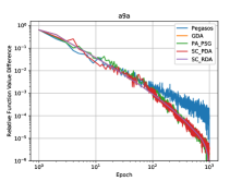
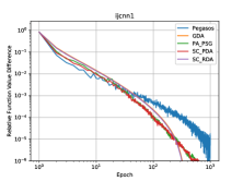
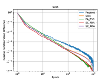
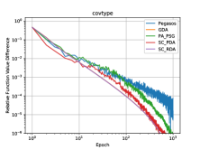
Figure 1: Convergence on different LibSVM datasets for SVMs

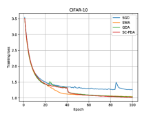
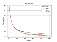
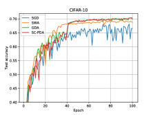
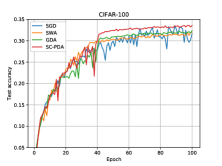
Figure 2: Training loss and test accuracy on CIFAR-10 and CIFAR-100 datasets for deep learning tasks

Figure 1. exposes how the relative function values $f(\mathbf{w}_{t})-f(\mathbf{w_{*}})$ are changed with respect to the algorithm epoch. As expected, the convergence behavior of our proposed GDA and SC-PDA is very similar to PA-PSG and SC-RDA with the same strong convexity parameter, and lower than Pegasos. Intuitively, the proposed SC-PDA, Pegasos and PA-PSG have almost the same convergence behavior with oscillation, which result from non-averaging scheme. Thus, we derive conclusions that our proposed two algorithms no longer suffer from the additional logarithmic factor and achieve their desired optimal rate.

Training Deep Neural Networks

The second experiment is to show that the proposed algorithms improve the performance of training deep networks. Interestingly, averaging in deep learning has been discussed in a series work about SWA. But they have not observed that the connection between DA and GD with averaging scheme. Moreover, averaging scheme does good for the convergence behavior of the gradient-based methods in terms of individual iterate instead of averaged output. According to the choice of $a_{t}$ and $\gamma_{t}$ in the Corollary 2, it should be mentioned that we use the different weighted averaging scheme in GDA and SC-PDA.

Following (Izmailov et al. 2018; Mukkamala and Hein 2017; Wang et al. 2020), we conduct experiments on a sever with 2 NVIDIA 2080Ti GPUs. We first design a simple 4-layer CNN architecture that consists two convolutional layers (32 filters of size 3 $\times$ 3), one max-pooling layer (2 $\times$ 2 window and 0.25 dropout) and one fully connected layer (128 hidden units and 0.5 dropout). We also use weight decay with a regularization parameter of 5e-3. The loss function is the cross-entropy. To conduct a fair comparison, the constant learning rate is tuned in {0.1; 0.01; 0.001; 0.0001}, and the best results are reported. The training loss and test accuracy are shown in Figure 2.

Our SC-PDA, GDA and SWA obtain almost the same training loss, lower than SGD (without momentum) on CIFAR-10 and CIFAR-100 datasets. Moreover, the improved performance also translates into good result on test accuracy. The performance of test accuracy gives our SC-PDA and GDA a slight edge over SGD and SWA. Compared to SGD, averaging schemes always reduce oscillation issues and achieve improvement in better generalization. Although our proposed GDA and SC-PDA are designed for strongly convex functions, it could also lead to practical performance even in some non-convex deep learning tasks.

Conclusion

In this paper, our original intention is to derive the optimal individual convergence of DA in the strongly convex case. We first propose a general algorithm GDA and we further slightly modify Nesterov’s PDA into SC-PDA. We prove that GDA yields the optimal convergence rate in terms of OA, while SC-PDA derives the optimal individual convergence.

Averaging scheme has been frequently employed in modern machine learning community for improving stability and generalization. Unfortunately, there is still a lack of valuable hints how various parameters should be chosen so far. Our proposed GDA and SC-PDA algorithms not only fix the optimal convergence issues but also lead to better performance in deep learning tasks.

Supplementary Material

Proof of Theorem 1

According to the strong convexity of $f$ (Definition 1) and 3-point property,

$$\sum_{k=0}^{t}a_{k}\nabla f(\mathbf{w}_{k})-\sum_{k=0}^{t}a_{k}\nabla f(\mathbf{w})$$

$$\leq\sum_{k=0}^{t}\langle a_{k}\nabla f(\mathbf{w}_{k}),\mathbf{w}_{k}-\mathbf{w}\rangle-\frac{\mu}{2}\sum_{k=0}^{t}a_{k}\|\mathbf{w}_{k}-\mathbf{w}\|^{2}-\frac{\mu}{2}\sum_{k=0}^{t}\gamma_{k}\|\mathbf{w}_{k}-\mathbf{w}\|^{2}+\frac{\mu}{2}\sum_{k=0}^{t}\gamma_{k}\|\mathbf{w}_{k}-\mathbf{w}\|^{2}$$

$$\leq\sum_{k=0}^{t}\langle a_{k}\nabla f(\mathbf{w}_{k}),\mathbf{w}_{k}-\mathbf{w}_{t+1}\rangle-\frac{\mu}{2}\sum_{k=0}^{t}\gamma_{k}\|\mathbf{w}_{k}-\mathbf{w}_{t+1}\|^{2}-\frac{\mu}{2}\sum_{k=0}^{t}\gamma_{k}\|\mathbf{w}-\mathbf{w}_{t+1}\|^{2}+\frac{\mu}{2}\sum_{k=0}^{t}(\gamma_{k}-a_{k})\|\mathbf{w}_{k}-\mathbf{w}\|^{2}.$$

Note that $\sum_{k=0}^{t}\langle a_{k}\nabla f(\mathbf{w}_{k}),\mathbf{w}_{k}-\mathbf{w}\rangle-\frac{\mu}{2}\sum_{k=0}^{t}\gamma_{k}\|\mathbf{w}_{k}-\mathbf{w}\|^{2}$ is the objective function of optimization problems in GDA. Then, we consider the following two terms,

$$\sum_{k=0}^{t}\langle a_{k}\nabla f(\mathbf{w}_{k}),\mathbf{w}_{k}-\mathbf{w}_{t+1}\rangle-\frac{\mu}{2}\sum_{k=0}^{t}\gamma_{k}\|\mathbf{w}_{k}-\mathbf{w}_{t+1}\|^{2}$$

$$=\sum_{k=0}^{t-1}\langle a_{k}\nabla f(\mathbf{w}_{k}),\mathbf{w}_{k}-\mathbf{w}_{t+1}\rangle-\frac{\mu}{2}\sum_{k=0}^{t-1}\gamma_{k}\|\mathbf{w}_{k}-\mathbf{w}_{t+1}\|^{2}+\langle a_{t}\nabla f(\mathbf{w}_{t}),\mathbf{w}_{t}-\mathbf{w}_{t+1}\rangle-\frac{\mu}{2}\gamma_{t}\|\mathbf{w}_{t}-\mathbf{w}_{t+1}\|^{2}$$

$$\leq\sum_{k=0}^{t-1}\langle a_{k}\nabla f(\mathbf{w}_{k}),\mathbf{w}_{k}-\mathbf{w}_{t}\rangle-\frac{\mu}{2}\sum_{k=0}^{t-1}\gamma_{k}\|\mathbf{w}_{k}-\mathbf{w}_{t}\|^{2}-\frac{\mu}{2}\sum_{k=0}^{t-1}\gamma_{k}\|\mathbf{w}_{t}-\mathbf{w}_{t+1}\|^{2}$$

$$+\langle a_{t}\nabla f(\mathbf{w}_{t}),\mathbf{w}_{t}-\mathbf{w}_{t+1}\rangle-\frac{\mu}{2}\gamma_{t}\|\mathbf{w}_{t}-\mathbf{w}_{t+1}\|^{2}$$

$$\leq\big{[}\sum_{k=0}^{t-1}\langle a_{k}\nabla f(\mathbf{w}_{k}),\mathbf{w}_{k}-\mathbf{w}_{t}\rangle-\frac{\mu}{2}\sum_{k=0}^{t-1}\gamma_{k}\|\mathbf{w}_{k}-\mathbf{w}_{t}\|^{2}\big{]}+\langle a_{t}\nabla f(\mathbf{w}_{t}),\mathbf{w}_{t}-\mathbf{w}_{t+1}\rangle-\frac{\mu}{2}\sum_{k=0}^{t}\gamma_{k}\|\mathbf{w}_{t}-\mathbf{w}_{t+1}\|^{2}.$$

Further, we can combine last two items with Fenchel-Young inequality, such that

$$a_{t}\langle\nabla f(\mathbf{w}_{t}),\mathbf{w}_{t}-\mathbf{w}_{t+1}\rangle-\frac{\mu}{2}\sum_{k=0}^{t}\gamma_{k}\|\mathbf{w}_{t}-\mathbf{w}_{t+1}\|^{2}\leq\frac{a_{t}^{2}}{2\mu\Gamma_{t}}\|\nabla f(\mathbf{w}_{t})\|^{2},$$

where $\Gamma_{t}=\sum_{k=0}^{t}\gamma_{k}$. Applying recursively this inequality, we can get

$$\frac{1}{A_{t}} \sum_{k=0}^{t}a_{k}f(\mathbf{w}_{k})-f(\mathbf{w}_{*})\leq\frac{1}{A_{t}}\sum_{k=0}^{t}\frac{a_{k}^{2}}{2\mu\Gamma_{k}}\|\nabla f(\mathbf{w}_{k})\|^{2}+\frac{\mu}{2A_{t}}\sum_{k=0}^{t}(\gamma_{k}-a_{k})\|\mathbf{w}_{k}-\mathbf{w}\|^{2}$$

Thus, Theorem 1 is proved.

Proof of Lemma 3

According to the step of PA, we note that

$$a_{t}(\mathbf{w}_{t}-\mathbf{w}_{t-1}^{+})=A_{t-1}\left(\mathbf{w}_{t-1}-\mathbf{w}_{t}\right),$$

then let’s multiply both sides by $\nabla f(\mathbf{w}_{t})$, and the left side of the above equality becomes

$$a_{t}\langle\nabla f(\mathbf{w}_{t}),\mathbf{w}_{t}-\mathbf{w}_{t}^{+}\rangle=a_{t}\langle\nabla f(\mathbf{w}_{t}),\mathbf{w}_{t}-\mathbf{w}_{t-1}^{+}\rangle+a_{t}\langle\nabla f(\mathbf{w}_{t}),\mathbf{w}_{t-1}^{+}-\mathbf{w}_{t}^{+}\rangle,$$

Next, let’s consider the first inner product term,

$$a_{t}\langle\nabla f(\mathbf{w}_{t}),\mathbf{w}_{t}-\mathbf{w}_{t-1}^{+}\rangle$$

$$=A_{t-1}\langle\nabla f(\mathbf{w}_{t}),\mathbf{w}_{t-1}-\mathbf{w}_{t}\rangle$$

$$\leq A_{t-1}f(\mathbf{w}_{t-1})-A_{t-1}f(\mathbf{w}_{t})-\dfrac{\mu}{2}A_{t-1}\|\mathbf{w}_{t-1}-\mathbf{w}_{t}\|^{2}.$$

Finally, we have

$$a_{t}\langle\nabla f(\mathbf{w}_{t}),\mathbf{w}_{t}-\mathbf{w}_{t}^{+}\rangle$$

$$=a_{t}\langle\nabla f(\mathbf{w}_{t}),\mathbf{w}_{t}-\mathbf{w}_{t-1}^{+}\rangle+a_{t}\langle\nabla f(\mathbf{w}_{t}),\mathbf{w}_{t-1}^{+}-\mathbf{w}_{t}^{+}\rangle$$

$$=A_{t-1}\langle\nabla f(\mathbf{w}_{t}),\mathbf{w}_{t}-\mathbf{w}_{t-1}\rangle+a_{t}\langle\nabla f(\mathbf{w}_{t}),\mathbf{w}_{t-1}^{+}-\mathbf{w}_{t}^{+}\rangle$$

$$\leq A_{t-1}[f(\mathbf{w}_{t-1})-f(\mathbf{w}_{t})]+a_{t}\langle\nabla f(\mathbf{w}_{t}),\mathbf{w}_{t-1}^{+}-\mathbf{w}_{t}^{+}\rangle.$$

Lemma 3 is proved.

Proof of Theorem 2

Similar to the proof of Theorem 1,

$$\sum_{k=1}^{t}a_{k}\nabla f(\mathbf{w}_{k})-\sum_{k=1}^{t}a_{k}\nabla f(\mathbf{w})$$

$$\leq\sum_{k=1}^{t}\langle a_{k}\nabla f(\mathbf{w}_{k}),\mathbf{w}_{k}-\mathbf{w}\rangle-\frac{\mu}{2}\sum_{k=1}^{t}a_{k}\|\mathbf{w}_{k}-\mathbf{w}\|^{2}-\frac{\mu}{2}\sum_{k=1}^{t}\gamma_{k}\|\mathbf{w}_{k}-\mathbf{w}\|^{2}+\frac{\mu}{2}\sum_{k=1}^{t}\gamma_{k}\|\mathbf{w}_{k}-\mathbf{w}\|^{2}$$

$$\leq\sum_{k=1}^{t}\langle a_{k}\nabla f(\mathbf{w}_{k}),\mathbf{w}_{k}-\mathbf{w}_{t}^{+}\rangle-\frac{\mu}{2}\sum_{k=1}^{t}\gamma_{k}\|\mathbf{w}_{k}-\mathbf{w}_{t}^{+}\|^{2}-\frac{\mu}{2}\sum_{k=1}^{t}\gamma_{k}\|\mathbf{w}-\mathbf{w}_{t}^{+}\|^{2}+\frac{\mu}{2}\sum_{k=1}^{t}(\gamma_{k}-a_{k})\|\mathbf{w}-\mathbf{w}_{t}^{+}\|^{2}.$$

Next, we consider the first two terms,

$$\sum_{k=0}^{t}\langle a_{k}\nabla f(\mathbf{w}_{k}),\mathbf{w}_{k}-\mathbf{w}_{t}^{+}\rangle-\frac{\mu}{2}\sum_{k=0}^{t}\gamma_{k}\|\mathbf{w}_{k}-\mathbf{w}_{t}^{+}\|^{2}$$

$$=\sum_{k=1}^{t-1}\langle a_{k}\nabla f(\mathbf{w}_{k}),\mathbf{w}_{k}-\mathbf{w}_{t}^{+}\rangle-\frac{\mu}{2}\sum_{k=0}^{t-1}\gamma_{k}\|\mathbf{w}_{k}-\mathbf{w}_{t}^{+}\|^{2}-\frac{\mu}{2}\gamma_{t}\|\mathbf{w}_{t}-\mathbf{w}_{t}^{+}\|^{2}+\langle a_{t}\nabla f(\mathbf{w}_{t}),\mathbf{w}_{t}-\mathbf{w}_{t}^{+}\rangle$$

$$\leq\sum_{k=1}^{t-1}\langle a_{k}\nabla f(\mathbf{w}_{k}),\mathbf{w}_{k}-\mathbf{w}_{t-1}^{+}\rangle-\frac{\mu}{2}\sum_{k=0}^{t-1}\gamma_{k}\|\mathbf{w}_{k}-\mathbf{w}_{t-1}^{+}\|^{2}-\frac{\mu}{2}\sum_{k=0}^{t-1}\gamma_{k}\|\mathbf{w}_{t}^{+}-\mathbf{w}_{t-1}^{+}\|^{2}$$

$$+\langle a_{t}\nabla f(\mathbf{w}_{t}),\mathbf{w}_{t}-\mathbf{w}_{t}^{+}\rangle-\frac{\mu}{2}\gamma_{t}\|\mathbf{w}_{t}-\mathbf{w}_{t}^{+}\|^{2}$$

Then, according to Lemma 3, we have

$$\leq\sum_{k=1}^{t-1}\langle a_{k}\nabla f(\mathbf{w}_{k}),\mathbf{w}_{k}-\mathbf{w}_{t-1}^{+}\rangle-\frac{\mu}{2}\sum_{k=0}^{t-1}\gamma_{k}\|\mathbf{w}_{k}-\mathbf{w}_{t-1}^{+}\|^{2}-\frac{\mu}{2}\sum_{k=0}^{t-1}\gamma_{k}\|\mathbf{w}_{t}^{+}-\mathbf{w}_{t-1}^{+}\|^{2}$$

$$-\frac{\mu}{2}\gamma_{t}\|\mathbf{w}_{t}^{+}-\mathbf{w}_{t-1}^{+}\|^{2}+\langle a_{t}\nabla f(\mathbf{w}_{t}),\mathbf{w}_{t-1}^{+}-\mathbf{w}_{t}^{+}\rangle+A_{t-1}\big{[}f(\mathbf{w}_{t-1})-f(\mathbf{w}_{t})\big{]}$$

$$\leq A_{t-1}\big{[}f(\mathbf{w}_{t-1})-f(\mathbf{w}_{t})\big{]}+\big{[}\sum_{k=0}^{t-1}\langle a_{k}\nabla f(\mathbf{w}_{k}),\mathbf{w}_{k}-\mathbf{w}_{t-1}^{+}\rangle-\frac{\mu}{2}\sum_{k=0}^{t-1}\gamma_{k}\|\mathbf{w}_{k}-\mathbf{w}_{t-1}^{+}\|^{2}\big{]}$$

$$+\big{[}a_{t}\langle\nabla f(\mathbf{w}_{t}),\mathbf{w}_{t-1}^{+}-\mathbf{w}_{t}^{+}\rangle-\frac{\mu}{2}\Gamma_{t}\|\mathbf{w}_{t}^{+}-\mathbf{w}_{t-1}^{+}\|^{2}\big{]}$$

$$\leq A_{t-1}\big{[}f(\mathbf{w}_{t-1})-f(\mathbf{w}_{t})\big{]}+\big{[}\sum_{k=0}^{t-1}\langle a_{k}\nabla f(\mathbf{w}_{k}),\mathbf{w}_{k}-\mathbf{w}_{t-1}^{+}\rangle-\frac{\mu}{2}\sum_{k=0}^{t-1}\gamma_{k}\|\mathbf{w}_{k}-\mathbf{w}_{t-1}^{+}\|^{2}\big{]}$$

$$+\frac{a_{t}^{2}}{2\mu\Gamma_{t}}\|\nabla f(\mathbf{w}_{t})\|^{2}$$

Then applying recursively this inequality for $A_{t}[f(\mathbf{w}_{t})-f(\mathbf{w})]$, Theorem 2 is proved.

Proof of Corollary 3

Note that

$$\bar{\mathbf{w}}_{t}=\dfrac{1}{t}\sum_{i=0}^{n}\mathbf{w}_{i}$$

is called standard averaging scheme in mathematics. According to Corollary 2 (1) and using the property of Harmonic Serie, we can get

$$f(\bar{\mathbf{w}}_{t})-f(\mathbf{w}_{*})\leq O\left(\frac{\log t}{t}\right).$$

Thus, Corollary 2 is proved.

Proof of Theorem 3

We just easily replace the gradient operation $\nabla f(\mathbf{w}_{t})$ with $\hat{\mathbf{g}}_{t}$ in the stochastic setting, because of theoretical guarantees (Rakhlin, Shamir, and Sridharan 2011). Therefore, we can have

$$\mathbb{E}[f(\mathbf{w}_{t})-f(\mathbf{w})]\leq\frac{1}{A_{t}}\sum_{k=0}^{t}\frac{a_{k}^{2}}{2\mu\Gamma_{k}}\|\hat{\mathbf{g}}_{t}\|^{2}+\frac{\mu}{2A_{t}}\sum_{k=0}^{t}(\gamma_{k}-a_{k})\|\mathbf{w}_{k}-\mathbf{w}\|^{2}.$$

Then, Let $a_{t}=\gamma_{t}=t$, it holds that

$$\mathbb{E}[f(\mathbf{w}_{t})-f(\mathbf{w})]\leq O\left(\frac{1}{t}\right).$$

Theorem 3 can be proved.

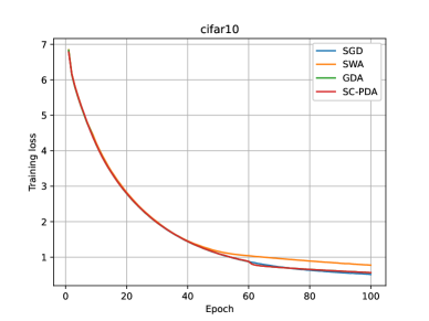
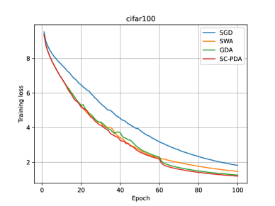
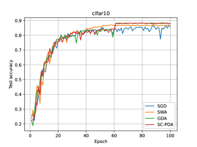
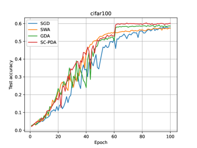
Figure 3: Training loss and test accuracy on CIFAR-10 and CIFAR-100 datasets for VGG-16

Additional Experiment Results

To further emphasize the performance of our proposed GDA and SC-PDA, we also conduct experiments on standard VGG-16. For fair comparison, the constant learning rate is tuned in {0.1; 0.05; 0.01; 0.005; 0.001} and the best results are reported. We also repeat each experiment five times and take their average results. As can be seen in figure 3, the performance of our proposed GDA and SC-PDA is better than that of SWA and SGD. We obtain the conclusion that algorithms coupled with averaging schemes in deep learning always reduce oscillation issues and achieve improvement in test accuracy.

References

• Athiwaratkun et al. (2018) Athiwaratkun, B.; Finzi, M.; Izmailov, P.; and Wilson, A. G. 2018. There are many consistent explanations of unlabeled data: Why you should average. In International Conference on Learning Representations.
• Beck and Teboulle (2003) Beck, A.; and Teboulle, M. 2003. Mirror descent and nonlinear projected subgradient methods for convex optimization. Operations Research Letters 31(3): 167–175.
• Chen, Lin, and Pena (2012) Chen, X.; Lin, Q.; and Pena, J. 2012. Optimal regularized dual averaging methods for stochastic optimization. In Advances in Neural Information Processing Systems, 395–403.
• Cutkosky (2019) Cutkosky, A. 2019. Anytime online-to-batch, optimism and acceleration. In International Conference on Machine Learning, 1446–1454.
• Defazio and Gower (2020) Defazio, A.; and Gower, R. M. 2020. Factorial powers for stochastic optimization. arXiv preprint arXiv:2006.01244 .
• Dekel et al. (2012) Dekel, O.; Gilad-Bachrach, R.; Shamir, O.; and Xiao, L. 2012. Optimal distributed online prediction using mini-batches. The Journal of Machine Learning Research 13: 165–202.
• Dimitri P., Angelia., and Asuman E. (2003) Dimitri P., B.; Angelia., N.; and Asuman E., O. 2003. Convex analysis and optimization. Athena Scientific.
• Flammarion and Bach (2017) Flammarion, N.; and Bach, F. 2017. Stochastic composite least-squares regression with convergence rate O (1/n). arXiv preprint arXiv:1702.06429 .
• Guo et al. (2020) Guo, Z.; Wu, Z.; Yan, Y.; Wang, X.; and Yang, T. 2020. Revisiting SGD with increasingly weighted averaging: optimization and generalization Perspectives. arXiv preprint arXiv:2003.04339 .
• Harvey et al. (2019) Harvey, N. J.; Liaw, C.; Plan, Y.; and Randhawa, S. 2019. Tight analyses for non-smooth stochastic gradient descent. In Conference on Learning Theory, 1579–1613.
• Harvey, Liaw, and Randhawa (2019) Harvey, N. J.; Liaw, C.; and Randhawa, S. 2019. Simple and optimal high-probability bounds for strongly-convex stochastic gradient descent. arXiv preprint arXiv:1909.00843 .
• Hazan et al. (2006) Hazan, E.; Kalai, A.; Kale, S.; and Agarwal, A. 2006. Logarithmic regret algorithms for online convex optimization. In International Conference on Computational Learning Theory, 499–513. Springer.
• Hazan and Kale (2011) Hazan, E.; and Kale, S. 2011. Beyond the regret minimization barrier: an optimal algorithm for stochastic strongly-convex optimization. In Proceedings of the Annual Conference on Learning Theory, 421–436.
• Izmailov et al. (2018) Izmailov, P.; Podoprikhin, D.; Garipov, T.; Vetrov, D.; and Wilson, A. G. 2018. Averaging weights leads to wider optima and better generalization. arXiv preprint arXiv:1803.05407 .
• Jain, Nagaraj, and Netrapalli (2019) Jain, P.; Nagaraj, D.; and Netrapalli, P. 2019. Making the last iterate of SGD information theoretically optimal. In Conference on Learning Theory, 1752–1755.
• Joulani et al. (2020) Joulani, P.; Raj, A.; György, A.; and Szepesvári, C. 2020. A simpler approach to accelerated stochastic optimization: iterative averaging meets optimism. In Proceedings of the International Conference on Machine learning.
• Kingma and Ba (2014) Kingma, D. P.; and Ba, J. 2014. Adam: A method for stochastic optimization. arXiv preprint arXiv:1412.6980 .
• Lacoste-Julien, Schmidt, and Bach (2012) Lacoste-Julien, S.; Schmidt, M.; and Bach, F. 2012. A simpler approach to obtaining an O (1/$t$) convergence rate for the projected stochastic subgradient method. arXiv preprint arXiv:1212.2002 .
• Ma and Yarats (2018) Ma, J.; and Yarats, D. 2018. Quasi-hyperbolic momentum and adam for deep learning. arXiv preprint arXiv:1810.06801 .
• Maddox et al. (2019) Maddox, W. J.; Izmailov, P.; Garipov, T.; Vetrov, D. P.; and Wilson, A. G. 2019. A simple baseline for bayesian uncertainty in deep learning. In Advances in Neural Information Processing Systems, 13153–13164.
• Mukkamala and Hein (2017) Mukkamala, M. C.; and Hein, M. 2017. Variants of Rmsprop and Adagrad with logarithmic regret bounds. In International Conference on Machine Learning.
• Nemirovsky and Yudin (1983) Nemirovsky, A. S.; and Yudin, D. B. 1983. Problem complexity and method efficiency in optimization. John Wiley $\&$ Sons .
• Nesterov (1983) Nesterov, Y. 1983. A method of solving a convex programming problem with convergence rate $O(1/k^{2})$ 27(2): 372–376.
• Nesterov (2009) Nesterov, Y. 2009. Primal-dual subgradient methods for convex problems. Mathematical programming 120(1): 221–259.
• Nesterov and Shikhman (2015) Nesterov, Y.; and Shikhman, V. 2015. Quasi-monotone subgradient methods for nonsmooth convex minimization. Journal of Optimization Theory and Applications 165(3): 917–940.
• Polyak and Juditsky (1992) Polyak, B. T.; and Juditsky, A. B. 1992. Acceleration of stochastic approximation by averaging. SIAM journal on control and optimization 30(4): 838–855.
• Rakhlin, Shamir, and Sridharan (2011) Rakhlin, A.; Shamir, O.; and Sridharan, K. 2011. Making gradient descent optimal for strongly convex stochastic optimization. arXiv preprint arXiv:1109.5647 .
• Reddi, Kale, and Kumar (2019) Reddi, S. J.; Kale, S.; and Kumar, S. 2019. On the convergence of adam and beyond. arXiv preprint arXiv:1904.09237 .
• Shalev-Shwartz, Singer, and Srebro (2007) Shalev-Shwartz, S.; Singer, Y.; and Srebro, N. 2007. Pegasos: primal estimated sub-gradient solver for SVM. In Proceedings of the international conference on Machine learning, 807–814.
• Shamir (2012) Shamir, O. 2012. Open problem: Is averaging needed for strongly convex stochastic gradient descent? In Conference on Learning Theory, 47–1.
• Shamir and Zhang (2013) Shamir, O.; and Zhang, T. 2013. Stochastic gradient descent for non-smooth optimization: Convergence results and optimal averaging schemes. In International conference on machine learning, 71–79.
• Tao et al. (2020) Tao, W.; Pan, Z.; Wu, G.; and Tao, Q. 2020. Primal averaging: A new gradient evaluation step to attain the optimal individual convergence. IEEE Transactions on Cybernetics 50(2): 835–845.
• Taylor and Bach (2019) Taylor, A.; and Bach, F. 2019. Stochastic first-order methods: non-asymptotic and computer-aided analyses via potential functions. In Conference on Learning Theory, 2934–2992.
• Wang et al. (2020) Wang, G.; Lu, S.; Tu, W.; and Zhang, L. 2020. Sadam: A variant of adam for strongly convex functions. In International Conference on Learning Representations.
• Xiao (2009) Xiao, L. 2009. Dual averaging method for regularized stochastic learning and online optimization. In Advances in Neural Information Processing Systems, 2116–2124.
• Yang et al. (2019) Yang, G.; Zhang, T.; Kirichenko, P.; Bai, J.; Wilson, A. G.; and De Sa, C. 2019. Swalp: Stochastic weight averaging in low-precision training. arXiv preprint arXiv:1904.11943 .