Memory-dependent noise-induced resonance and diffusion in non-markovian systems

Abstract

We study the random processes with non-local memory and obtain new solutions of the Mori-Zwanzig equation describing non-markovian systems. We analyze the system dynamics depending on the amplitudes $\nu$ and $\mu_{0}$ of the local and non-local memory and pay attention to the line in the ($\nu$, $\mu_{0}$)-plane separating the regions with asymptotically stationary and non-stationary behavior. We obtain general equations for such boundaries and consider them for three examples of the non-local memory functions. We show that there exist two types of the boundaries with fundamentally different system dynamics. On the boundaries of the first type, the diffusion with memory takes place, whereas on borderlines of the second type, the phenomenon of noise-induced resonance can be observed. A distinctive feature of noise-induced resonance in the systems under consideration is that it occurs in the absence of an external regular periodic force. It takes place due to the presence of frequencies in the noise spectrum, which are close to the self-frequency of the system. We analyze also the variance of the process and compare its behavior for regions of asymptotic stationarity and non-stationarity, as well as for diffusive and noise-induced-resonance borderlines between them.

I Introduction

The Markov processes are the simplest and the most popular models for describing the random phenomena (see, e.g., Refs. Zaburdaev et al. (2013); Rebenshtok et al. (2014); Ferialdi (2016); Nickelsen and Touchette (2018); Uhlenbeck and Ornstein (1930); Van Kampen (1992); Gardiner (1985); Horsthemke (1984)). A lot of systems in the real world are more complex than the markovian ones, they have non-markovian character of the memory (see, e.g., Refs. Mokshin et al. (2005); Breuer and Vacchini (2008); Sarracino et al. (2010); Siegle et al. (2010); Rosvall et al. (2014); Starnini et al. (2017); Cáceres (1999); van Kampen (1998)). Therefore, it is necessary to go beyond the simple markovian model. In recent years, a lot of attention has been paid to studying the non-Markov processes, in particular, due to their role in decoherence phenomena in open quantum systems (see, e.g., Refs. Lambropoulos et al. (2000); Breuer and Vacchini (2008); Kang et al. (2011)). Namely, non-markovianity can serve as a source for suppressing the exponential decay of coherence in the interaction of a quantum system with a classical thermal bath Bellomo et al. (2007); Chin et al. (2012); Bylicka et al. (2014).

In formulation of what is the Markov process, very important role is played by its exponential correlation function. As was shown in Refs. Hanggi et al. (1978); Nakazawa (1966), the replacement of the exponential correlation function by another one leads to the non-stationarity of the process. A particular class of strongly non-markovian stochastic processes with long-range correlated noise appearing in the corresponding stochastic differential equation (SDE) was studied in Refs. Wang and Tokuyama (1999); Goychuk (2012). McCauley McCauley (2010) considered the non-stationary non-markovian processes with 1-state memory where the SDE takes into account the value of random variable $V$ at fixed temporal point $t_{0}$ in the past.

The difficulties arising in attempts to introduce a correlation function different from exponential are closely connected with two facts: a desire to determine the conditional probability distribution function (CPDF) for arbitrary time laps $\tau$ from the last known value of random variable and to determine a group chain rule for the CPDF. To overcome these difficulties, we have introduced in Ref. Melnyk et al. (2019) integral memory term depending on the past of the process into the SDE and the transition probability function. Thus, we refused to deal with the CPDF for arbitrary value $\tau$ and considered the case of infinitesimal $\tau=dt\rightarrow 0$ only.

Introduction of the integral memory term results in transformation of the SDE into the stochastic integro-differential equation (SIDE),

$$dV(t) = -\nu V(t)dt$$

$$- \int_{0}^{\infty}\mu(t^{\prime})V(t-t^{\prime})dt^{\prime}dt+\sigma\,dW(t).$$

Here $dW(t)$ is the standard white noise, i.e., $W(t)$ is the continuous centered Wiener process with independent increments with variance $\langle(W(t+\tau)-W(t))^{2}\rangle=|\tau|$, or, equivalently, $W(t)=\int dW(t)\Rightarrow$ $\langle dW(t)dW(t^{\prime})\rangle=\delta(t-t^{\prime})dtdt^{\prime}$, the symbol $\langle...\rangle$ denotes a statistical ensemble averaging. The term $-\nu V(t)dt$ in Eq. (I) describes a local-memory one-point feature of the process. The positive value of the constant $\nu$ provides an anti-persistent character of the process with attraction of $V(t)$ to the point $V=0$. If we omit the memory term $\mu(t^{\prime})$ in Eq. (I), then we obtain the well known equation for the Ornstein-Uhlenbeck process, which simulates the Brownian motion of a microscopic particle in a liquid viscous suspension subjected to a random force with intensity $\sigma$. Equation (I) is often named as the Mori-Zwanzig one Mori (1965); Zwanzig (1960, 2001), or the external-regular-force-independent generalized Langevin equation Goychuk (2012). The Mori-Zwanzig equation (I) finds numerous applications (see, e.g., Ref. te Vrugt and Wittkowski (2019) and references therein).

Such generalization of SDE has also been discussed by many authors Adelman (1976); Hänggi and Thomas (1982); Hynes (1986); Wang and Tokuyama (1999). In most cases, the so-called internal noise was considered, when, according to the fluctuation-dissipation theorem Toda et al. (1991), the function $\mu(t)$ is uniquely determined by the correlation function of the stochastic perturbation $W(t)$. Then the memory kernel $\mu(t)$ describes the so-called viscoelastic friction Goychuk (2012). However, in the case of external noise, the fluctuation and dissipation come from different sources, i.e., the frictional kernel $\mu(t)$ and the correlation function of the noise are independent of each other (see, e.g., Ref. Wang and Tokuyama (1999)).

In this paper we consider an arbitrary memory kernel $\mu(t)$ and a Gaussian external noise $W(t)$ independent of $\mu(t)$. In this case Eq. (I) could be a good physical model for the systems where the external noise is much more intensive than the thermal one.

Our general consideration of the Mory-Zwanzig equation is accompanied by the model examples of the memory functions. The first example is the local memory function defined at the time moment $(t-T)$ remote at the depth $T$ from the instant time moment $t$,

$$\mu(t)=\frac{\mu_{0}}{T}\delta(t-T).$$ (2)

Here $\delta(.)$ denotes the Dirac delta, $\mu_{0}$ is the memory amplitude. To produce the random value of $V(t+dt)$ the system “uses” the knowledge about its past in the points $t$ and $t-T$. This memory function is a good approximation for any process with a pronounced maximum in the $\mu(t)$ dependence at $t=T$.

The second example is the step-wise memory function Usatenko and Yampol’skii (2003); Usatenko et al. (2009),

$$\mu(t)=\frac{\mu_{0}}{T^{2}}\theta(T-t),$$ (3)

where $\theta(.)$ is the Heaviside theta-function. This function is a good approximation for any process with a pronounced edge in the $\mu(t)$ dependence at $t=T$.

At last, we show that Eq. (I) has an exact analytical solution for the memory function of the exponential form,

$$\mu(t)=\frac{\mu_{0}}{T^{2}}\exp(-t/T).$$ (4)

Note that the exponential memory function can be used to describe many real physical phenomena, e.g., the coupling of a massive tracer with the surrounding granular fluid Sarracino et al. (2010). This model describes qualitatively any other processes with smoothly decreasing memory function. Thus, the considered here three examples of memory functions describe qualitatively the most typical kinds of the $\mu(t)$ dependences, regardless of their physical implementations.

The dynamics of the system described by Eq. (I) is very sensitive to the region in which the parameters $\mu_{0}$ and $\nu$ are located. In particular, it was shown in our previous work Melnyk et al. (2019) that the process with the delta-functional memory is asymptotically stationary not for any values of $\mu_{0}$ and $\nu$. It is very interesting and nontrivial that, for example, for $\nu=0$, there are two boundaries of asymptotic stationarity, $\mu_{0}=0$ and $\mu_{0}=\mu_{\mathrm{crit}}=2/\pi$. Approaching the lower boundary, we observe the ordinary Brownian diffusion. Approaching the upper boundary, for $\mu_{0}\rightarrow\mu_{\mathrm{crit}}$, the process goes into the oscillation mode with a certain fixed frequency of oscillations. The analysis of Eqs. (11), which are presented in the next Section, shows that similar two boundaries of stationarity exist for any system with arbitrary memory function $\mu(t)$.

In this paper, we study the system dynamics in various regions of the parameters $\mu_{0}$ and $\nu$ with the main focus on the boundaries of the region of asymptotic stationarity. We show that there are two types of such boundaries with fundamentally different system behavior. On the boundaries of the first type, corresponding to smaller values of $\mu_{0}$, a diffusion with non-local memory takes place, and we call these borderlines as diffusive. On the boundaries of the second type, corresponding to larger values of $\mu_{0}$, the phenomenon of noise-induced resonance occurs.

The scope of the paper is as follows. In the next section, we obtain general expressions for the boundaries of the region of asymptotic stationarity in the $(\nu,\mu_{0})$-plane, and present these boundaries for the above mentioned three examples of memory functions.

In Section III, we analyze the behavior of the system for different prehistories in various areas in the $(\nu,\mu_{0})$-plain in the absence of random force. We show that, on the upper borderline of the asymptotic stationarity region, the variable $V(t)$ goes asymptotically into an oscillatory mode with some given frequency. This means that we deal here with the system with well-defined frequency of self-oscillations. On the lower borderline , the variable $V$ tends to a constant value at $t\rightarrow\infty$.

Section IV is the main in our paper. Here we show that the switching on the random force in the Mori-Zwanzig system leads to the diffusion on the lower boundary of asymptotic stationarity and to the noise-induced resonance at the upper boundary. A distinctive feature of the noise-induced resonance in the systems under consideration is that it occurs in the absence of an external regular periodic force. It takes place due to the presence of frequencies in the noise spectrum, which are close to the self-frequency of the system. Then we study the variance of the process and compare its behavior for regions of asymptotic stationarity and non-stationarity, as well as for diffusion and noise-induced-resonance boundaries between them.

II Boundaries of asymptotic stationarity

The random process under study is very sensitive to the values of two memory parameters, $\nu$ and $\mu_{0}$. In this section, we analyze the borderlines of region in the $(\nu,\mu_{0})$-plain where the process is asymptotically stationary. In this region, the two-point correlation function $C(t_{1},t_{2})$,

$$C(t_{1},t_{2})=\langle V(t_{1})V(t_{2})\rangle-\langle V(t_{1})\rangle\langle V(t_{2})\rangle,$$ (5)

is asymptotically dependent on the difference $t_{2}-t_{1}\equiv t$ only, i.e., $C(t_{1},t_{2})\approx C(t)$ at $t_{1},t_{2}\rightarrow\infty$:

$$C(t)=\lim_{t^{\prime}\rightarrow\infty}C(t^{\prime},t^{\prime}+t).$$ (6)

Herein the time difference $t$ can be arbitrary.

As was shown in Ref. Melnyk et al. (2019), the correlation function $C(t)$ of the process is governed by the continuous analog of the Yule-Walker equation, Yule (1927); Walker (1931),

$$\frac{dC(t)}{dt}+\nu C(t)+\int_{0}^{\infty}\mu(t^{\prime})C(t-t^{\prime})dt^{\prime}=0,\quad t>0,$$ (7)

with the boundary condition,

$$\frac{dC(t)}{dt}{\Big{|}_{t=0_{+}}}=-\frac{\sigma^{2}}{2}.$$ (8)

The argument $0_{+}$ signifies that the derivative is taken at positive $t$ close to zero. The simple method to obtain Eq. (7) is presented in Appendix A.

Two equations, (7) and (8), represent a very useful tool for studying the statistical properties of random processes with non-local memory. These properties are governed by the constants $\nu$, $\sigma$, and the memory function $\mu(t)$. We assume that the function $\mu(t)$ has good properties at $t\rightarrow\infty$. More exactly, we suppose that the function $\mu(t)$ has either a finite characteristic scale $T$ of decrease, or it abruptly vanishes at $t>T$, $\mu(t>T)=0$. In this case, the correlation function can be presented as a sum of exponential terms,

$$C(t)=\sum_{i}C_{i}\exp\left(-\frac{z_{i}t}{T}\right),$$ (9)

for $t\gg T$.

Equation (7) gives the following characteristic algebraic equation for the complex decrements $z_{i}$:

$$\frac{z}{T}=\nu+\int_{0}^{\infty}\mu(t)\exp\left(\frac{zt}{T}\right)dt.$$ (10)

Solving it, we find a set of $z_{i}$ as functions of the parameters $\nu$ and $\mu_{0}$. We are interested in the root $z_{0}$ of Eq. (10) with the lowest real part because specifically this root defines behavior of the correlation function Eq. (9) at $t\rightarrow\infty$. From Eq. (9), one can see that the imaginary part of $z_{0}=\xi_{0}+i\zeta_{0}$ corresponds to the oscillations of $C(t)$, while the sign of its real part, $\xi_{0}$, defines the stationarity properties. The positive $\xi_{0}$ corresponds to the exponential decrease of the correlation function $C(t)$, and the negative value of $\xi_{0}$ does to the exponential increase.

Thus, to find the borderline of stationary range in the $(\nu,\mu_{0})$-plain, we should solve Eq. (10) for the purely imaginary $z=i\zeta$. In this case Eq. (10) gives

$$\begin{cases}\nu+\int_{0}^{\infty}\mu(t)\cos\left(\dfrac{\zeta t}{T}\right)\;dt=0,\\[8.0pt] \dfrac{\zeta}{T}-\int_{0}^{\infty}\mu(t)\sin\left(\dfrac{\zeta t}{T}\right)\;dt=0.\end{cases}$$ (11)

Let us apply the set of Eqs. (11) for investigating the stationarity borderlines in the frame of the mentioned above three models of the non-local memory $\mu(t)$.

II.0.1 Delta-functional memory

As the first example, we consider the memory function $\mu(t)=(\mu_{0}/T)\delta(t-T)$. Then, Eq. (11) transforms into

$$\begin{cases}\nu T+\mu_{0}\cos\zeta=0,\\[5.0pt] \zeta-\mu_{0}\sin\zeta=0.\end{cases}$$ (12)

For $0<\zeta<\pi$ this set of equations describes the so called “oscillatory” borderline because the corresponding correlation function $C(t)$, Eq. (9), oscillates without damping when approaching this borderline. In the case $\zeta\rightarrow 0$, the $C(t)$ function tends very smoothly to zero without oscillations in the vicinity of stationarity borderline. Assuming $\zeta=0$ in Eq. (12), we get for this borderline,

$$\nu T+\mu_{0}=0.$$ (13)

Figure 1 shows the oscillatory (upper red curve) and diffusive (lower straight black line) stationarity borderlines.

Note that the general equation, valid for arbitrary memory function, describing the diffusive borderline, can easily be obtained if we put $\zeta=0$ in Eqs. (11),

$$\nu+\int_{0}^{\infty}\mu(t)dt=0.$$ (14)

If $\int_{0}^{\infty}\mu(t)dt\neq 0$, we can define the amplitude $\mu_{0}$ of the memory function as

$$\mu_{0}=T\int_{0}^{\infty}\mu(t)dt.$$ (15)

Then Eq. (13) for the diffusive borderline will be valid for any memory function.

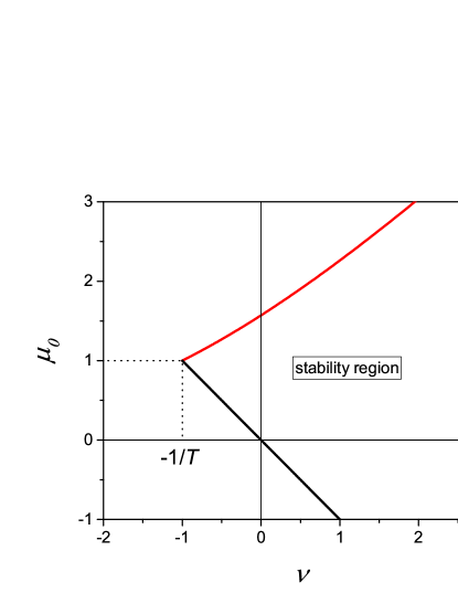
Figure 1: The stationarity borderlines for the delta-functional memory $\mu(t)=(\mu_{0}/T)\delta(t-T)$ with $T=1$ in the plane $(\nu,\mu_{0})$. The red solid curve at $\mu_{0}>1$ corresponds to the oscillatory borderline, and the black solid straight line does to the diffusive one.

II.0.2 Step-wise memory function

As the second example, we consider the step-wise memory function $\mu(t)=(\mu_{0}/T^{2})\theta(T-t)$. From the same considerations as above, we obtain the following relations:

$$\begin{cases}\nu=-\dfrac{1}{T}\dfrac{\zeta\sin\zeta}{1-\cos\zeta},\\[6.0pt] \mu_{0}=\dfrac{\zeta^{2}}{1-\cos\zeta},\qquad 0\leqslant\zeta<2\pi,\end{cases}$$ (16)

for the oscillatory borderline and Eq. (13) for the diffusive one. These two borderlines are shown in Fig. 2.

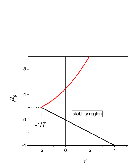
Figure 2: The stationarity borderlines for the step-wise memory function $\mu(t)=(\mu_{0}/T^{2})\theta(T-t)$ with $T=0.5$ in the plane $(\nu,\mu_{0})$. The upper red solid curve is the oscillatory borderline, and the lower black solid straight line at $\mu_{0}<2$ is the diffusive one.

II.0.3 Exponential memory function

As the third example, we consider the exponential memory function $\mu(t)=(\mu_{0}/T^{2})\exp(-t/T)$ with the positive memory depth $T$. Then the condition for the diffusive borderline is Eq. (13). For the oscillatory borderline we have

$$\begin{cases}\nu=-\dfrac{1}{T},\\ \mu_{0}=1+\zeta^{2}.\end{cases}$$ (17)

These two borderlines are shown in Fig. 3.

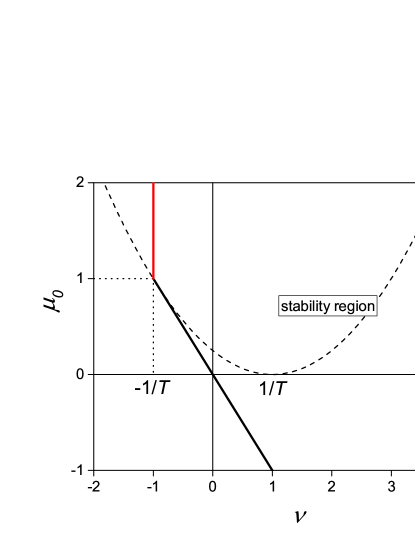
Figure 3: The stationarity borderlines for the exponential memory function $\mu(t)=(\mu_{0}/T^{2})\exp(-t/T)$ with $T=1$ in the plane $(\nu,\mu_{0})$. The region of stationarity lies to the right of the solid line, the region of non-stationarity lies to the left of this line. The vertical red and oblique black solid lines correspond to the oscillatory and diffusive borderlines, respectively. A dashed parabola separates the areas where the correlation function decays exponentially without oscillations (below the parabola) and with oscillations (above this curve).

Thus, the results obtained in this Section are as follows:

• The correlation function $C(t)$ of the random process with non-local memory can be presented as a sum of exponential functions with the complex decrements/increments $z_{i}$ defined by Eq. (10).

• The stationarity of the process is defined by the root $z_{0}$ of Eq. (10) with the smallest real part. If $\xi_{0}=\Re z_{0}>0$, then the function $C(t\rightarrow\infty)$ tends to zero, and the stochastic process $V(t)$ is stationary. If $\xi_{0}<0$, then the process $V(t)$ is non-stationary.

• The condition $\xi_{0}=0$ defines the borderlines between the stationary and non-stationary regions in the ($\nu$, $\mu_{0}$)-plain. There exist two types of borderlines, diffusive and oscillatory ones. The diffusive borderline corresponds to the case when the imaginary part of $z_{0}$ equals zero, $\zeta_{0}=\Im z_{0}=0$. This borderline is described by Eq. (14) (see black solid straight lines in Figs. 1, 2, and 3 for the examples considered above). The oscillatory borderline corresponds to $\zeta_{0}\neq 0$ and is described by Eq. (11) (see red solid curves in Figs. 1, 2, and 3 for the examples considered above).

• When approaching the diffusive borderline, the random process goes to the diffusion with memory and the decrement of $C(t)$ tends to zero. Approaching the oscillatory borderline, the correlation function goes into the oscillation mode with a certain frequency of oscillations.

• The conditions of stationarity for the process are independent of the random-force intensity $\sigma$.

III Movement in the absence of random force

In this Section, we analyze the system dynamics for different prehistories (i.e., for different $V(t)$ dependences at $t\leqslant 0$) in various areas of the $(\nu,\mu_{0})$-plain in the absence of random force. We show that, on the diffusive borderline, the variable $V(t\rightarrow\infty)$ reaches the constant value. On the oscillatory borderline, the variable $V(t\rightarrow\infty)$ goes into oscillatory mode with some given frequency. This means that in the latter case we deal with the specific linear oscillatory system.

III.1 Exact fundamental solution

The exact fundamental solution of deterministic (without external random force $dW(t)$) version of Eq. (I),

$$\frac{dV(t)}{dt}=-\nu V(t)-\int_{0}^{\infty}\mu(t^{\prime})V(t-t^{\prime})dt^{\prime},$$ (18)

with the fundamental prehistory,

$$V(t\leqslant 0)=\begin{cases}0,&t<0,\\ 1,&t=0,\end{cases}$$ (19)

can be found by the method of Laplace transformation (see, e.g., Ref. Wang and Tokuyama (1999)). Denoting this solution by $h(t)$ and performing the Laplace transformation of Eq. (18), we obtain the image $\tilde{h}(p)$ in the form,

$$\tilde{h}(p)=\int_{0}^{\infty}h(t)\exp(-p\,t)dt=\frac{1}{p+\nu+\tilde{\mu}(p)},$$ (20)

where $\tilde{\mu}(p)$ is the Laplace image of the memory function $\mu(t)$. The function $h(t)$ is determined by the inverse Laplace transformation,

$$h(t)=\frac{1}{2\pi i}\int_{\lambda-i\infty}^{\lambda+i\infty}\tilde{h}(p)\exp(p\,t)dp,\quad\lambda>0.$$ (21)

In our following calculations, the function $h(t)$ plays the role similar to the role of fundamental solutions (the Green functions) in the theory of differential equations. Therefore, we call it as the fundamental one.

It is important to emphasize that the poles $p=p_{i}$ of the function $\tilde{h}(p)$ coincide with the roots $z=z_{i}$ of the characteristic equation (10) up to the multiplier $-1/T$. This means that the fundamental solution $h(t)$ is represented as a sum of the same exponential terms as the correlation function $C(t)$. This remark applies to the stationarity region of parameters $\nu$ and $\mu_{0}$ only, where the correlation function $C(t)$ exists. In particular, the behaviors of functions $h(t)$ and $C(t)$ at $t\rightarrow\infty$ are the same, $h(t)\propto C(t)\propto\exp(-z_{0}t/T)$. Remind that $z_{0}$ is the root of Eq. (10) with the minimal real part.

III.2 Solution for the case of arbitrary prehistory

In this subsection we find the solution of the homogeneous deterministic equation (18) for the general prehistory of the process,

$$V(t\leqslant 0)=\begin{cases}V_{<}(t),&t<0,\\ V(0),&t=0.\end{cases}$$ (22)

The integral $\int_{0}^{\infty}dt^{\prime}\mu(t^{\prime})V(t-t^{\prime})$ in Eq. (18) can be presented as a sum of two terms, $\int_{0}^{t}dt^{\prime}\mu(t^{\prime})V(t-t^{\prime})$ and $\int_{-\infty}^{0}dt^{\prime\prime}\mu(t-t^{\prime\prime})V_{<}(t^{\prime\prime})$. The first one is the ordinary memory term containing integration from the “beginning $t^{\prime}=0$ of the process history” to the instant moment of time $t^{\prime}=t$. The second integral,

$$\int_{-\infty}^{0}dt^{\prime\prime}\mu(t-t^{\prime\prime})V_{<}(t^{\prime\prime})\equiv Z(t),$$ (23)

contains integration over the prehistory. It should be considered as the known function $Z(t)$.

After such a representation of the integral in Eq. (18), the deterministic version of the SIDE takes the form,

$$\dfrac{dV(t)}{dt}=-\nu V(t)-\int_{0}^{\infty}dt^{\prime}\mu(t^{\prime})V(t-t^{\prime})-Z(t).$$ (24)

This equation is supplemented by the specific prehistory,

$$V(t\leqslant 0)=\begin{cases}0,&t<0,\\ V(0),&t=0.\end{cases}$$ (25)

Now the actual prehistory $V_{<}(t)$ is taken into account by the additional regular force $-Z(t)$ in Eq. (24).

Applying the Laplace transformation to Eq. (24), we get,

$$\tilde{V}(p)=\dfrac{V(0)-\tilde{Z}(p)}{p+\nu+\tilde{\mu}(p)}=\tilde{h}(p)(V(0)-\tilde{Z}(p)).$$ (26)

Thus, the account for the prehistory of process leads to the only change of the fundamental solution, namely, to the appearance of additional term $Z(p)$ in the numerator of Eq. (26). As expected, the expression for $\tilde{V}(p)$ contains all the poles $p_{i}$ which define the fundamental solution.

III.3 Solution for the case of exponential memory function

In this subsection, we present in the explicit form an analytical solution of Eq. (18) with the exponential memory function, Eq. (4). The Laplace image of this memory function is

$$\tilde{\mu}(p)=\dfrac{\mu_{0}}{T}\dfrac{1}{1+p\,T},$$ (27)

which gives only two poles for $\tilde{h}(p)$ in Eq. (20). These poles are $p_{1,2}=-z_{1,2}/T$ with

$$z_{1,2}=\frac{1+\nu T}{2}\pm\sqrt{\frac{(1-\nu T)^{2}}{4}-\mu_{0}}.$$ (28)

For the sake of simplicity we consider here the prehistory Eq. (25). Using the inverse Laplace transformation, Eq. (21), we find the solution,

$$\frac{V(t)}{V(0)}=A_{1}\exp{(-z_{1}t/T)}+A_{2}\exp{(-z_{2}t/T)},$$ (29)

with

$$A_{1}=\frac{1-z_{1}}{z_{2}-z_{1}},\quad A_{2}=\frac{1-z_{2}}{z_{1}-z_{2}}.$$ (30)

The analysis of poles, Eq. (28), shows that, if the parameters $\nu$ and $\mu_{0}$ satisfy the condition,

$$\mu_{0}=\frac{(1-\nu T)^{2}}{4},$$ (31)

the poles $z_{1}$ and $z_{2}$ coincide, i.e., the degeneration takes place. In this case, the solution has the form,

$$V(t)=V(0)\left(1-\dfrac{1-\nu T}{2T}t\right)\exp{(-zt/T)},$$ (32)

where $z={(1+\nu T)}/{2}$. The parabola, Eq. (31), is shown by the dashed line in Fig.3. At $\mu_{0}>(1-\nu T)^{2}/4$, above the parabola, the exponential decrease of $V(t)$ is accompanied by oscillations. These oscillations are absent below the parabola.

Comparing Eqs. (28), (29) with Eq. (9), one can see that the solution $V(t)$ decreases exponentially in the same region where the random process is stationary and the correlation function exists. Wherein, the asymptotic behavior of the function $V(t\rightarrow\infty)$ and $C(t\rightarrow\infty)$ coincides. This is not surprising. Indeed, the equations for these functions are the same, the only difference consists in the initial conditions, see Eqs. (8) and (19). The memory about these conditions is asymptotically lost at $t\rightarrow\infty$ and thus, the asymptotic solutions for $V(t\rightarrow\infty)$ and $C(t\rightarrow\infty)$ coincide.

In the region of parameters $\nu$ and $\mu_{0}$ located to the left of the solid lines in Fig.3, the solution $V(t)$ exponentially increases. We are most interested in the $V(t)$ behavior on the borderlines between the stationary and non-stationary regions. On the diffusive borderline, $\mu_{0}+\nu T=0$, the pole $z_{2}$ in Eq. (28) vanishes, and the solution Eq. (29) for $V(t)$ goes asymptotically to the constant value $A_{2}$. For the oscillatory borderline, $\nu T=-1,\,\mu_{0}>1$, Eqs. (28), (29), and (30) give the harmonic solution for $V(t)$,

$$V(t)=V(0)\left[\cos(\omega t)+\frac{1}{\omega T}\sin(\omega t)\right],\,\omega=\frac{1}{T}\sqrt{\mu_{0}-1}.$$ (33)

Another method, presented in Refs. van Kampen (1998); Puglisi and Villamaina (2009), to solve Eq. (18) with exponential memory function consists in introducing a new auxiliary variable $U(t)=\int_{-\infty}^{t}V(t^{\prime})\exp[-(t-t^{\prime})/T]dt^{\prime}$. This procedure maps the system under consideration onto a Markov process, which is described by two ordinary differential equations. In the absence of random force, these equations have the form,

$$\begin{cases}\frac{dV(t)}{dt}=-\nu V(t)-\frac{\mu_{0}}{T^{2}}U(t),\\[6.0pt] \frac{dU(t)}{dt}=V(t)-\frac{1}{T}U(t).\end{cases}$$ (34)

In the case of prehistory Eq. (25), the set of equations (34) is supplemented by the initial conditions, $V(t=0)=V(0)$ and $U(t=0)=0$. Solving Eqs. (34) with these initial conditions one can easily obtain results Eq. (28) — (33). Besides, the analysis of the stability region and oscillatory/simple decay of the correlation functions in this region, provided in this paper for the case of exponential memory function, is equivalent to the study of the eigenvalues of the coupling matrix between the variables $V(t)$ and $U(t)$.

A similar asymptotic behavior of $V(t)$ in the different regions of $(\nu,\mu_{0})$-plain takes place not only for the system with exponential memory function but for other systems with arbitrary $\mu(t)$ having a well-defined memory depth $T$.

IV Movement under the action of random force

At the beginning of this section, we show by numerical simulations that, taking into account the random force in the Mori-Zwanzig equation, one can observe the diffusion with memory on the lower borderline of stationarity and the noise-induced resonance on the upper borderline. Then we analyze the variance $D(t)$ which characterizes conveniently the correlation properties of the stochastic systems and compare the behavior of this function in various domains in the $(\nu,\mu_{0})$-plane.

IV.1 Numerical simulations

The account of the $\sigma dW(t)$-term in Eq. (I) allows one to describe the stochastic features of the process under consideration. It does not change the location of stationarity borderlines, they can still be defined by analyzing the correspondent deterministic dynamical equation. This is the consequence of the fact that the Gaussian noise can neither limit an exponentially increasing solution in the non-stationarity region, nor overcome the attraction effects in the stationarity zone. However, the stochastic force changes the system dynamics, especially on the stationarity borderlines.

Irregular thin black solid lines in Fig. 4 show several realizations of the diffusion motion for the Mori-Zwanzig equation with exponential memory function and the zero prehistory $V(t\leqslant 0)=0$. The parameters $\nu,T$, and $\mu_{0}$ are chosen to satisfy the condition $\nu T+\mu_{0}=0$. At first glance, this memory-dependent diffusion does not differ from the usual Brownian motion. However, there exists an essential difference. To demonstrate this difference, we carried out the ensemble averaging of $V^{2}(t)$ over $10^{3}$ realizations. The obtained dependence $\pm\sqrt{D(t)}=\pm\sqrt{\langle V^{2}(t)\rangle}$ is plotted by the red symbols on the green solid line. In addition, we present the similar plot for the Brownian diffusion by the red dashed curve. The comparison of these two curves shows that the memory dependent diffusion follows the usual Brownian motion at small time scale $t\ll T$ only. This coincidence at short times is not surprising. It is due to the chosen zero prehistory. However, at $t\gtrsim T$ the memory begins to play the important role in the diffusion. Therefore, the green solid curve in Fig. 4 deviates from the Brownian red dashed line and tends to another asymptote with a greater diffusion coefficient.

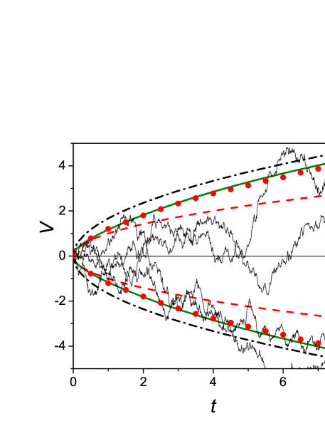
Figure 4: The memory dependent diffusion for the exponential memory function and zero prehistory $V(t\leqslant 0)=0$. The irregular black solid lines are the trajectories for different realizations of the stochastic process $V(t)$ on the diffusive borderline of stationarity. The green solid line is the analytical result for $\pm\sqrt{D(t)}$ where $D(t)$ is the variance, Eq. (42). The red symbols on this curve are the results of numerical simulation obtained by the ensemble averaging over $10^{3}$ realizations for each symbol. The dashed red line presents the $\pm\sqrt{D_{\,\texttt{B}}(t)}=\pm\sigma\sqrt{t}$ dependence for the Brownian diffusion. The dash-dotted curve is the dependence $\pm\sigma\sqrt{t}/(1+\nu T)$ which serves as the asymptote for $\pm\sqrt{D(t)}$ at $t\gg T$, see Eqs. (42) and (IV.2.3). The parameters are: $\nu=-0.4$, $\mu_{0}=0.4$, $T=1$, and $\sigma=1$.

Figure 5 demonstrates the oscillatory motion with increasing amplitude for the Mori-Zwanzig system under the action of random force. This motion occurs with the frequency close to the frequency of self-oscillations, Eq. (33). The Fourier analysis made for a 6000-length realization of the process gives an estimate $\Delta\omega/\omega\sim 0.04$ for the relative width of frequency domain of these oscillations. This means that we deal with a kind of the noise-induced resonance.

One of the most frequently discussed types of amplification of oscillations due to external noise is the stochastic resonance (see, e.g., Refs. Benzi et al. (1981); Gammaitoni et al. (1998); McDonnell et al. (2008) and references therein). Usually, stochastic resonance is considered for the nonlinear systems with double-well potentials in the presence of an external regular periodic force, and resonance occurs when the frequency of the external force is comparable with half the characteristic frequency of the noise-induced interwell transitions. In the system we are considering, there are neither double-well potentials, nor an external periodic force. In our case, the noise does “double duty”. The inclusion of noise leads, firstly, to the resonant excitation of oscillations at the self-frequency $\omega$, Eq. (33). This takes place due to the presence of frequencies in the noise spectrum, which are close to $\omega$. Secondly, the noise leads to a subsequent increase in the amplitude of oscillations over time. The discussed here phenomenon resembles the well-known coherence resonance which is also observed in the absence of an external regular periodic force Pikovsky and Kurths (1997). However, contrary to the coherence resonance, we consider here the linear systems where the noise-induced resonance occurs due to their memory of the prehistory.

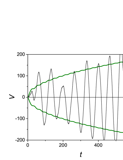
Figure 5: The noise-induced resonance in the $V(t)$ process with the exponential memory function and zero prehistory. The thin black solid line shows a realization of the stochastic process $V(t)$ on the oscillatory borderline of stationarity. The green solid line presents the analytical result for $\pm\sqrt{D(t)}$, Eq. (45). The parameters are: $\nu=-1/T$, $\mu_{0}=1.01$, $T=1$, and $\sigma=1$.

IV.2 Analytical study of the $V(t)$ variance

One of the valuable characteristics of the stationary and non-stationary random process $V(t)$ is the variance,

$$D(t)=\langle V^{2}(t)\rangle-\langle V(t)\rangle^{2}.$$ (35)

The function $D(t)$ can be easily obtained by means of the exact solution of the Mori-Zwanzig equation (I),

$$V(t)=V(0)h(t)+\sigma\int_{0}^{t}h(t-\tau)dW(\tau),$$ (36)

(see, e.g., Ref. Wang and Tokuyama (1999)). This formula is valid for the specific prehistory, Eq. (25).

Using the definition Eq. (35) and the property of the white noise $\langle dW(t)dW(t^{\prime})\rangle=\delta(t-t^{\prime})dtdt^{\prime}$, we express the variance $D(t)$ in terms of the fundamental solution $h(t)$,

$$D(t)=\sigma^{2}\int_{0}^{t}h^{2}(\tau)d\tau+V^{2}(0)[h(t)-1]^{2}.$$ (37)

We analyze Eq. (37) considering different regions of parameters $\nu$ and $\mu_{0}$, specifically, the regions of stationarity, non-stationarity and the borderlines between them. As far as the main properties of solutions of the Mori-Zwanzig equation do not depend essentially on the initial value $V(0)=\langle V(t)\rangle$, we set it to be zero, $V(0)=0$, for simplicity. We carry out our analysis for the systems with exponential memory function.

IV.2.1 Stationarity region

In this region, the variance Eq. (37) increases with $t$ but remains finite even at $t\rightarrow\infty$,

$$D(\infty)=\sigma^{2}\int_{0}^{\infty}h^{2}(\tau)d\tau.$$ (38)

Indeed, the fundamental solution $h(t)$ exponentially decreases when increasing $t$, therefore the integral in Eq. (38) exists.

For the process with exponential memory function, we can carry out an analysis of the variance $D(t)$ in more details and obtain analytical expressions in explicit form. Substituting the function $h(t)$ from Eq. (29) into Eq. (37), after integration we get

$$D(t)=\sigma^{2}T\!\!\!\!\sum_{\!\!i,k=1,2}\!\!\!\dfrac{A_{i}A_{k}}{z_{i}+z_{k}}\left\{1-\exp\left[-(z_{i}+z_{k})\frac{t}{T}\right]\right\}.$$ (39)

At $t\rightarrow\infty$, the exponential function in this equation goes to zero and we obtain for $D(\infty)$,

$$D(\infty)=\frac{1}{2}\sigma^{2}T\dfrac{1+\mu_{0}+\nu T}{(\mu_{0}+\nu T)(1+\nu T)}.$$ (40)

As expected, the variance $D(\infty)$ diverges (tends to infinity) if the point $(\nu,\mu_{0})$ approaches the diffusive borderline (due to the first factor in the denominator of Eq. (40)) or the oscillatory borderline (due to the second factor in the denominator).

IV.2.2 Non-stationarity region

In the region of non-stationarity, at least one of the roots, $z_{1}$ or $z_{2}$ in Eq. (28) has the negative real part, say $-r$. Therefore, the main contribution to Eq. (39) gives the term proportional to $\exp{(2rt/T)}$. So, one should observe the exponential increase (possibly with oscillations) of the variance at $t\rightarrow\infty$.

IV.2.3 Solution on the diffusive borderline

On the line $\nu T+\mu_{0}=0$, one root in Eq. (28), say $z_{1}$, is real and positive, $z_{1}=1+\nu T=r>0$, and the other root is zero, $z_{2}=0$. Using $A_{1,2}$ in Eq. (30), we get the fundamental solution,

$$h(t)=\frac{\nu T}{1+\nu T}\exp(-rt/T)+\frac{1}{1+\nu T},$$ (41)

and the variance,

$$D(t)\!=\!a\,t\!+\!b\left[1-\exp(-rt/T)\right]\!+\!c\!\left[1-\exp(-2rt/T)\right]\!,$$ (42)

where

$$a=\frac{\sigma^{2}}{(1+\nu T)^{2}},\quad b=\frac{2\sigma^{2}\nu T^{2}}{(1+\nu T)^{3}},$$

$$c=\frac{\sigma^{2}\nu^{2}T^{3}}{2(1+\nu T)^{3}}.$$ (43)

The $D(t)$-dependence on the diffusive borderline $\nu T+\mu_{0}=0$ is shown in Fig. 6 for different values of $\mu_{0}$. One can see that all curves follow the same straight line $D(t)=\sigma^{2}t$ at $t\ll T$. This is explained by the mentioned above circumstance: the memory does not play an essential role in the diffusion at short time scales due to the chosen zero prehistory. Then, at $t\gtrsim T$, the $D(t)$ curves for $\mu(t)\neq 0$ leave the “brownian” asymptote $D(t)=\sigma^{2}t$ and go to the other asymptotes $D(t)=\sigma^{2}t/(1+\nu T)$. In the case of positive memory function $\mu(t)$, the curves $D(t)$ deviate upward, which corresponds to the persistent diffusion, and for negative $\mu(t)$ the curves deviate downward, which corresponds to the antipersistence.

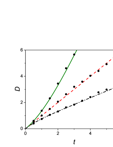
Figure 6: The variance $D(t)$ on diffusive borderline for the exponential memory function and zero prehistory at different values of $\mu_{0}$: $\mu_{0}=0.4$ (the upper green solid curve), $\mu_{0}=0$ (the red straight dashed line), and $\mu_{0}=-0.4$ (the lower black dash-dotted curve). The black filled circles on these curves are the results of numerical simulations obtained by the ensemble averaging over $10^{3}$ realizations for each symbol. Other parameters: $\nu=-\mu_{0}/T$, $T=1$, and $\sigma=1$.

IV.2.4 Solution on the noise-induced-resonance borderline

For the exponential memory function, on the oscillatory borderline (the vertical line in Fig. 3, $\nu=-1/T$, $\mu_{0}>1$ ), both roots, $z_{1}$ and $z_{2}=-z_{1}$, in Eq. (28)) are imaginary, $z_{1}=ir$, $z_{2}=-ir$, where $r=\sqrt{\mu_{0}-1}$. Using the coefficients in the fundamental solution Eq. (30),

$$A_{1}=\frac{r+i}{2r},\qquad A_{2}=\frac{r-i}{2r},$$ (44)

and Eqs. (39), (33), we get

$$D(t) =\frac{\sigma^{2}}{2\omega^{2}T}\left[\mu_{0}\frac{t}{T}+(\mu_{0}-2)\frac{\sin(2\omega t)}{2\omega T}\right.$$ (45)

$$\left.+1-\cos(2\omega t)\right],\quad\omega=\frac{1}{T}\sqrt{\mu_{0}-1}.$$

The dependence $\pm\sqrt{D(t)}$ for the noise-induced resonance occurring on the oscillatory borderline is shown by the green solid line in Fig. 5. One can see that, in accordance with Eq. (45), the oscillations of ${D(t)}$ occur at the frequency $2\omega$.

V Conclusion

We have studied the continuous random non-markovian processes with non-local memory and obtained new solutions of the Mori-Zwanzig equation describing them. We have analyzed the system dynamics depending on the amplitudes $\nu$ and $\mu_{0}$ of the local and non-local memories and payed attention to the line in the ($\nu$, $\mu_{0}$)-plane separating the regions with asymptotically stationary and non-stationary behavior. We have obtained general equations for such borderlines and considered them for three examples of the non-local memory functions. The first example is the local, but remote from the instant time moment $t$, memory function; the second example is the step-wise memory function; at last, we have indicated that Eq. (I) has an exact analytical solution for the memory function of the exponential form.

In this paper, we have focused mainly on the system dynamics on the borderlines of asymptotic stationarity. We have shown that there exist two types of such borderlines with fundamentally different system dynamics. On boundaries of the first type, corresponding to the smaller values of $\mu_{0}$, a diffusion with memory takes place, and on the boundaries of the second type, corresponding to the larger values of $\mu_{0}$, the phenomenon of noise-induced resonance occurs.

We have analyzed the dynamics of system for different prehistories in various areas on the $(\nu,\mu_{0})$-plain in the absence of random force. We have shown that, on the lower borderline of the asymptotic-stationarity region, the variable $V$ tends to a constant value at $t\rightarrow\infty$. On the upper borderline, the variable $V(t\rightarrow\infty)$ goes asymptotically into oscillatory mode with some given frequency. This means that we deal here with the classical oscillatory motion.

Then, we have considered the system behavior under the action of random force. We have shown that on borderlines of the first type, corresponding to smaller values of the amplitude $\mu_{0}$ of non-local memory, the diffusion with memory takes place, whereas on borderlines of the second type, corresponding to larger values of $\mu_{0}$, the phenomenon of noise-induced resonance occurs. A distinctive feature of noise-induced resonance in the systems under consideration is that it occurs in the absence of an external regular periodic force. It takes place due to the presence of frequencies in the noise spectrum, which are close to the self-frequency of the system.

We have analyzed also the variance of the process and compared its behavior for regions of asymptotic stationarity and non-stationarity, as well as for diffusive and noise-induced-resonance borderlines between them.

The main results of this paper are valid for the processes with arbitrary memory kernel $\mu(t)$, which is restricted by the condition $\lim_{\mathfrak{T}\rightarrow\infty}\int^{\mathfrak{T}}\mu(t)dt<\infty$. This means that our theory fails for the polynomial memory functions ($\mu(t)\propto t^{-\alpha}$ at $t\rightarrow\infty$ with $\alpha<1$) for which the integral does not converge. It would be interesting to generalize our consideration to the non-markovian systems with infinite memory lengths.

We have studied the memory dependent diffusion and noise-induced resonance for the case of delta-correlated external noise. It seems reasonable, in future, to study the discussed phenomena for a more general case of internal noise and long-range correlated noise (see, e.g., Refs. Wang and Tokuyama (1999); Goychuk (2012)). We believe that, in such systems, the noise-induced resonance will not only continue to take place, but will also acquire new interesting features.

Appendix A Continuous Yule-Walker equation

Here we present a simple derivation of Eq. (7) for the correlation function $C(t)$ of continuous stationary process.

The exact solution Eq. (36) of the Mori-Zwanzig equation allows us to find all statistical characteristics of the system including its correlation function. Using the definition Eq. (6) and the property of the white noise $\langle dW(t)dW(t^{\prime})\rangle=\delta(t-t^{\prime})dtdt^{\prime}$, we obtain after simple calculations the following result:

$$C(t)=\lim_{t^{\prime}\rightarrow\infty}C(t^{\prime},t^{\prime}+t)=\sigma^{2}\int_{0}^{\infty}h(\tau)h(\tau+t)d\tau.$$ (46)

Remind that the function $h(t)$ (with the fundamental prehistory, Eq. (19)) is the solution of the deterministic version of the Mori-Zwanzig equation,

$$\dot{h}(t)+\nu h(t)+\int_{0}^{t}h(t-\tau)\mu(\tau)d\tau=0.$$ (47)

Using the prehistory $h(t<0)=0$ of the fundamental solution, we can replace the upper limit of integration in Eq. (47) by $\infty$. Differentiating Eq. (46) with respect to $t$ and substituting $\dot{h}(\tau+t)$ from Eq. (47), we get the continuous analog of the Yule-Walker equation, Eq. (7).

References

- Zaburdaev et al. (2013) V. Zaburdaev, S. Denisov, and P. Hänggi, Phys. Rev. Lett. 110, 170604 (2013).
- Rebenshtok et al. (2014) A. Rebenshtok, S. Denisov, P. Hänggi, and E. Barkai, Phys. Rev. Lett. 112, 110601 (2014).
- Ferialdi (2016) L. Ferialdi, Phys. Rev. Lett. 116, 120402 (2016).
- Nickelsen and Touchette (2018) D. Nickelsen and H. Touchette, Phys. Rev. Lett. 121, 090602 (2018).
- Uhlenbeck and Ornstein (1930) G. E. Uhlenbeck and L. S. Ornstein, Phys. Rev. 36, 823 (1930).
- Van Kampen (1992) N. G. Van Kampen, Stochastic processes in physics and chemistry, vol. 1 (Elsevier, Amsterdam, 1992).
- Gardiner (1985) C. W. Gardiner, Handbook of Stochastic Methods for Physics, Chemistry, and the Natural Sciences, vol. 3 (Springer-Verlag, Berlin, 1985).
- Horsthemke (1984) W. Horsthemke, in Non-Equilibrium Dynamics in Chemical Systems, Proceedings of the International Symposium, edited by C. Vidal and A. Pacault (Springer-Verlag, Berlin, 1984), vol. 27 of Springer Series in Synergetics, pp. 150–160.
- Mokshin et al. (2005) A. V. Mokshin, R. M. Yulmetyev, and P. Hänggi, Phys. Rev. Lett. 95, 200601 (2005).
- Breuer and Vacchini (2008) H.-P. Breuer and B. Vacchini, Phys. Rev. Lett. 101, 140402 (2008).
- Sarracino et al. (2010) A. Sarracino, D. Villamaina, G. Gradenigo, and A. Puglisi, Europhysics Letters 92, 34001 (2010).
- Siegle et al. (2010) P. Siegle, I. Goychuk, and P. Hänggi, Phys. Rev. Lett. 105, 100602 (2010).
- Rosvall et al. (2014) M. Rosvall, A. V. Esquivel, A. Lancichinetti, J. D. West, and R. Lambiotte, Nature communications 5, 1 (2014).
- Starnini et al. (2017) M. Starnini, J. P. Gleeson, and M. Boguñá, Phys. Rev. Lett. 118, 128301 (2017).
- Cáceres (1999) M. O. Cáceres, Brazilian journal of physics 29, 125 (1999).
- van Kampen (1998) N. G. van Kampen, Brazilian Journal of Physics 28, 90 (1998).
- Lambropoulos et al. (2000) P. Lambropoulos, G. M. Nikolopoulos, T. R. Nielsen, and S. Bay, Rep. Prog. Phys. 63, 455 (2000).
- Kang et al. (2011) P. K. Kang, M. Dentz, T. Le Borgne, and R. Juanes, Phys. Rev. Lett. 107, 180602 (2011).
- Bellomo et al. (2007) B. Bellomo, R. LoFranco, and G. Compagno, Phys. Rev. Lett. 99, 160502 (2007).
- Chin et al. (2012) A. W. Chin, S. F. Huelga, and M. B. Plenio, Phys. Rev. Lett. 109, 233601 (2012).
- Bylicka et al. (2014) B. Bylicka, D. Chruściński, and S. Maniscalco, Scientific reports 4, 1 (2014).
- Hanggi et al. (1978) P. Hanggi, H. Thomas, H. Grabert, and P. Talkner, J. Stat. Phys. 18, 155 (1978).
- Nakazawa (1966) H. Nakazawa, Progress of Theoretical Physics Supplement 36, 172 (1966).
- Wang and Tokuyama (1999) K. Wang and M. Tokuyama, Physica A: Statistical Mechanics and its Applications 265, 341 (1999).
- Goychuk (2012) I. Goychuk, Adv. Chem. Phys. 150, 187 (2012).
- McCauley (2010) J. L. McCauley, Physics Procedia 3, 1659 (2010).
- Melnyk et al. (2019) S. S. Melnyk, V. A. Yampol’skii, and O. V. Usatenko, Phys. Rev. E 100, 052141 (2019).
- Mori (1965) H. Mori, Prog. Theor. Phys. 33, 423 (1965).
- Zwanzig (1960) R. Zwanzig, J. Chem. Phys. 33, 1338 (1960).
- Zwanzig (2001) R. Zwanzig, Nonequilibrium statistical mechanics (Oxford University Press, 2001).
- te Vrugt and Wittkowski (2019) M. te Vrugt and R. Wittkowski, Phys. Rev. E 99, 062118 (2019).
- Adelman (1976) S. A. Adelman, J. Chem. Phys. 64, 124 (1976).
- Hänggi and Thomas (1982) P. Hänggi and H. Thomas, Physics Reports 88, 207 (1982).
- Hynes (1986) J. T. Hynes, J. Phys. Chem. 90, 3701 (1986).
- Toda et al. (1991) M. Toda, R. Kubo, N. Saitō, N. Hashitsume, et al., Statistical physics II: nonequilibrium statistical mechanics, vol. 2 (Springer Science & Business Media, 1991).
- Usatenko and Yampol’skii (2003) O. V. Usatenko and V. A. Yampol’skii, Phys. Rev. Lett. 90, 110601 (2003).
- Usatenko et al. (2009) O. Usatenko, S. Apostolov, Z. Mayzelis, and S. Melnik, Random finite-valued dynamical systems: additive Markov chain approach (Cambridge Scientific, Cambridge, 2009).
- Yule (1927) G. U. Yule, Philosophical Transactions of the Royal Society of London. Series A, Containing Papers of a Mathematical or Physical Character 226, 267 (1927).
- Walker (1931) G. T. Walker, Proceedings of the Royal Society of London. Series A, Containing Papers of a Mathematical and Physical Character 131, 518 (1931).
- Puglisi and Villamaina (2009) A. Puglisi and D. Villamaina, Europhysics Letters 88, 30004 (2009).
- Benzi et al. (1981) R. Benzi, A. Sutera, and A. Vulpiani, Journal of Physics A: Mathematical and General 14, L453 (1981).
- Gammaitoni et al. (1998) L. Gammaitoni, P. Hänggi, P. Jung, and F. Marchesoni, Rev. Mod. Phys. 70, 223 (1998).
- McDonnell et al. (2008) M. D. McDonnell, N. G. Stocks, C. E. Pearce, and D. Abbott, Stochastic Resonance: from Suprathreshold Stochastic Resonance to Stochastic Signal Quantization (Cambridge University Press, 2008).
- Pikovsky and Kurths (1997) A. S. Pikovsky and J. Kurths, Phys. Rev. Lett. 78, 775 (1997).