Raman mapping of photodissociation regions

Abstract

Broad Raman-scattered wings of hydrogen lines can be used to map neutral gas illuminated by high-mass stars in star forming regions. Raman scattering transforms far-ultraviolet starlight from the wings of the $\text{Ly}\beta$ line ($1022\text{\,}\mathrm{\SIUnitSymbolAngstrom}$ to $1029\text{\,}\mathrm{\SIUnitSymbolAngstrom}$) to red visual light in the wings of the $\text{H}\alpha$ line ($6400\text{\,}\mathrm{\SIUnitSymbolAngstrom}$ to $6700\text{\,}\mathrm{\SIUnitSymbolAngstrom}$). Analysis of spatially resolved spectra of the Orion Bar and other regions in the Orion Nebula shows that this process occurs in the neutral photo-dissociation region between the ionization front and dissociation front. The inner Raman wings are optically thick and allow the neutral hydrogen density to be determined, implying $n(\mathrm{H^{0}})\approx${10}^{5}\text{\,}\mathrm{c}\mathrm{m}^{-3}$$ for the Orion Bar. Far-ultraviolet resonance lines of neutral oxygen imprint their absorption onto the stellar continuum as it passes through the ionization front, producing characteristic absorption lines at $6633\text{\,}\mathrm{\SIUnitSymbolAngstrom}$ and $6664\text{\,}\mathrm{\SIUnitSymbolAngstrom}$ with widths of order $2\text{\,}\mathrm{\SIUnitSymbolAngstrom}$. This is a unique signature of Raman scattering, which allows it to be easily distinguished from other processes that might produce broad $\text{H}\alpha$ wings, such as electron scattering or high-velocity outflows.

1 Introduction

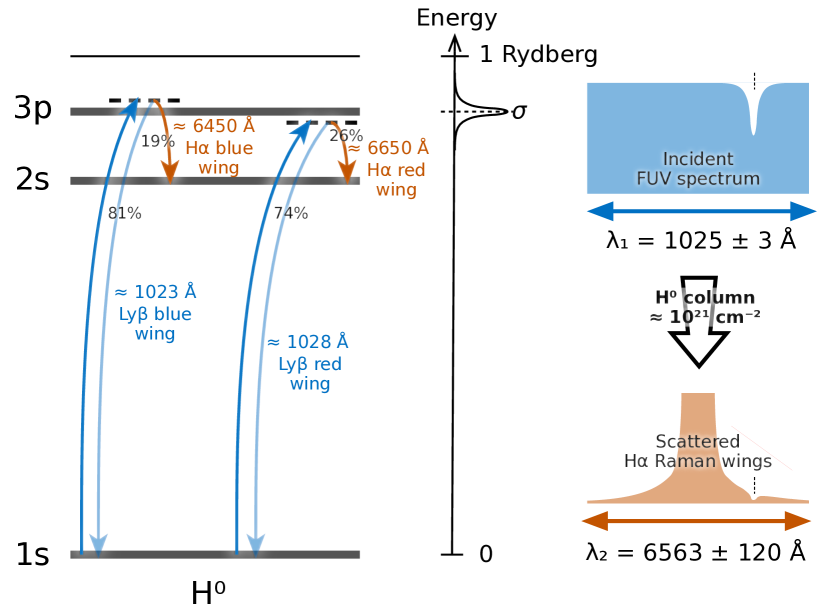
Figure 1: Schematic illustration of Raman scattering of photons from the $\text{Ly}\beta$ wings to the $\text{H}\alpha$ wings. The relevant energy levels of neutral hydrogen are shown at left. Far ultraviolet photons that are shifted by about $\Delta\lambda_{1}=\pm 1$ to $3\text{\,}\mathrm{\SIUnitSymbolAngstrom}$ from the $\text{Ly}\beta$ rest wavelength can excite transitions from the ground $\mathrm{1s}$ level to a virtual state adjacent to $\mathrm{3p}$. Most such excitations decay back to $\mathrm{1s}$ (Rayleigh scattering), but in about one-fifth of cases the decay is to $\mathrm{2s}$ instead (Raman scattering). The scattering cross section falls approximately as $\Delta\lambda_{1}^{-2}$, which gives broad Lorentzian wings to the $\text{H}\alpha$ line, as shown at right. A bandwidth of $\Delta\lambda_{1}=\pm$3\text{\,}\mathrm{\SIUnitSymbolAngstrom}$$ around $\text{Ly}\beta$ is transformed to a bandwidth $\Delta\lambda_{2}\approx\pm$120\text{\,}\mathrm{\SIUnitSymbolAngstrom}$$ around $\text{H}\alpha$. A narrow absorption line in the incident FUV spectrum (vertical thin dashed line) becomes a much broader notch in the scattered wings.

Raman scattering is the inelastic analog of Rayleigh scattering by atoms or molecules. Both processes begin with a radiation-induced transition of an electron to a virtual bound state (non-eigenstate). In Rayleigh scattering, the electron returns to its original state, resulting in the radiation being re-emitted with its original frequency (elastic scattering). In Raman scattering, on the other hand, the electron undergoes a transition to a different excited state, resulting in radiation being re-emitted at a much lower frequency. See Figure 1 for an illustration of the process. Recently, Dopita et al. (2016) identified exceedingly broad wings to the $\text{H}\alpha$ $6563\text{\,}\mathrm{\SIUnitSymbolAngstrom}$ line in the Orion Nebula and a number of $\mathrm{H\,\scriptstyle II}$ regions in the Magellanic Clouds, which they ascribe to Raman scattering of ultraviolet radiation in the vicinity of the $\text{Ly}\beta$ $1025\text{\,}\mathrm{\SIUnitSymbolAngstrom}$ transition. Raman scattering in astrophysical sources was first identified in symbiotic stars (Schmid, 1989), where FUV $\mathrm{O\,\scriptstyle VI}$ emission lines at $1032$ and $1038\text{\,}\mathrm{\SIUnitSymbolAngstrom}$ produce broad emission features at $6827$ and $7088\text{\,}\mathrm{\SIUnitSymbolAngstrom}$. This illustrates a curious feature of Raman scattering (Nussbaumer et al., 1989): the relative width $\Delta\lambda/\lambda$ of spectral features is amplified by a factor $\lambda(\text{H}\alpha)/\lambda(\text{Ly}\beta)\approx 6.4$ when passing from the FUV to the optical domain.

Dopita et al. (2016) propose that the Raman wings form at the transition zone near the ionization fronts in $\mathrm{H\,\scriptstyle II}$ regions. However, the total neutral hydrogen column through the ionization front can be no more than about $10/\sigma_{0}\approx$2\text{\times}{10}^{18}\text{\,}\mathrm{c}\mathrm{m}^{-2}$$, where $\sigma_{0}\approx$6.3\text{\times}{10}^{-18}\text{\,}\mathrm{c}\mathrm{m}^{2}$$ is the ground-state hydrogen photoionization cross section at threshold (Osterbrock & Ferland, 2006). The Raman scattering cross section at wavelengths responsible for the observed wings is much lower than this: $\sigma_{\text{Raman}}\sim${10}^{-21}\text{\,}\mathrm{c}\mathrm{m}^{2}$$ (Chang et al., 2015), meaning that the Raman scattering optical depth through the ionization front is only of order $0.001$. A vastly larger column density of neutral hydrogen ($\approx${10}^{21}\text{\,}\mathrm{c}\mathrm{m}^{-2}$$) is available in the photodissociation region (PDR) outside the ionization front, so it is more likely that Raman scattering will occur there instead, so long as there is sufficient far ultraviolet radiative flux.

This paper is organized as follows. Section 2 presents archival VLT-MUSE integral field spectroscopy of the Orion Nebula. Spectra of the broad H$\alpha$ wings are extracted for key areas of the nebula (section 2.1). Two components of the $\mathrm{O\,\scriptstyle I}$ UV resonance multiplet $\mathrm{2s2p^{4}\ {}^{3}P}\to\mathrm{2s2p^{3}3d\ ^{3}D^{o}}$ are detected as absorption features at $6633$ and $6664\text{\,}\mathrm{\SIUnitSymbolAngstrom}$ against the $\text{H}\alpha$ Raman wings (section 2.2). Three wavelength bands are defined in each of the red and blue wings that avoid contaminating emission and absorption features (section 2.3). The emission bands are spatially mapped and compared with other tracers of ionized and neutral zones in the nebula (section 2.4). Particular attention is paid to the edge-on photodissociation region at the Orion Bar (section 2.5). Equivalent widths of the Raman-scattered absorption lines are compared with the distribution of other absorption features in the nebula (section 2.6). Section 3 presents archival Keck-HIRES slit spectroscopy, which shows the profile of the $6664\text{\,}\mathrm{\SIUnitSymbolAngstrom}$ absorption line with an effective velocity resolution of $1\text{\,}\mathrm{k}\mathrm{m}\,\mathrm{s}^{-1}$. Section 4 discusses the implications of these results for the structure of the PDRs in Orion. An appendix recapitulates the basic theory of Raman scattering, concentrating on the wavelength transformation from the FUV domain around $\text{Ly}\beta$ to optical domain around $\text{H}\alpha$. In addition, polynomial fits are provided to the wavelength dependence of the total (Rayleigh plus Raman) scattering cross section and the Raman $\text{H}\alpha$ branching ratio.

2 Spectral mapping of Raman wings

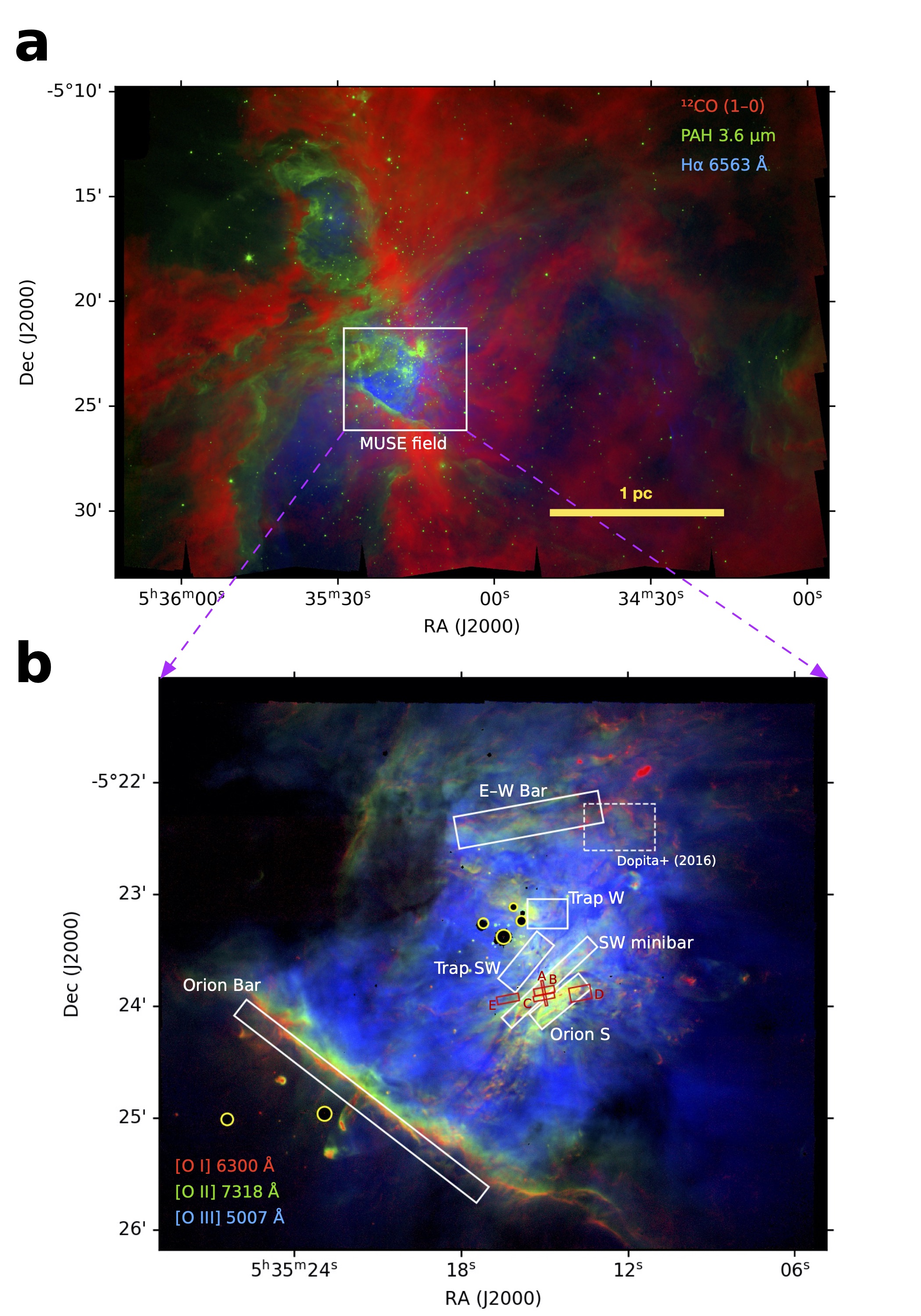
Figure 2: (a) Panoramic view of the Orion Nebula region on parsec scales. Red channel of background image shows $\mathrm{{}^{18}CO}$ emission from dense molecular gas Carma-NRO Orion Survey, Kong et al., 2018. Green channel shows near-infrared continuum from PAH grains in neutral gas Spitzer Orion Survey, Megeath et al., 2012. Blue channel shows optical H$\alpha$ emission from ionized gas WFI camera on ESO $2.2\text{\,}\mathrm{m}$ La Silla, Da Rio et al., 2009. The white box shows the field of view observed with MUSE. (b) Locations within the nebula of the extraction regions for the MUSE spectra shown in Figure 3 (white boxes) and the Keck HIRES spectra shown in Figure 10 (red boxes). The region of the spectrum obtained in Dopita et al. (2016) is shown by the dashed box. Background image shows oxygen emission lines extracted from the MUSE data cube: [$\mathrm{O\,\scriptstyle I}$] $\lambda 6300$ (red channel), which traces ionization fronts and shocks in neutral gas; [$\mathrm{O\,\scriptstyle II}$] $\lambda 7318$ (green channel), which traces the outer layers of the photoionized nebula; and [$\mathrm{O\,\scriptstyle III}$] $\lambda 5007$ (blue channel), which traces the highly ionized interior of the nebula.

The principal observational dataset used in this paper is the imaging spectroscopy mosaic of the inner Orion Nebula (Weilbacher et al., 2015; Mc Leod et al., 2016) obtained with the MUSE spectrograph (Bacon et al., 2010, 2014) on the VLT. The entire datacube covers the wavelength range $4595$ to $9366\text{\,}\mathrm{\SIUnitSymbolAngstrom}$ but we concentrate mainly on the range $6300$ to $6800\text{\,}\mathrm{\SIUnitSymbolAngstrom}$, where the spectral resolving power is $R\approx 2500$, corresponding to an instrumental linewidth (FWHM) of $\delta\lambda\approx$2.4\text{\,}\mathrm{\SIUnitSymbolAngstrom}$$, which is sampled at $1.25\text{\,}\mathrm{\SIUnitSymbolAngstrom}\,\mathrm{p}\mathrm{i}\mathrm{x}^{-1}$ and then resampled to $0.85\text{\,}\mathrm{\SIUnitSymbolAngstrom}\,\mathrm{p}\mathrm{i}\mathrm{x}^{-1}$ for the final calibrated cube see § 2 of Weilbacher et al., 2015. The observed field is shown by the white rectangle in Figure 2(a) and includes the entire inner Huygens region of the nebula, which accounts for roughly half of the total radio continuum flux from the $\mathrm{H\,\scriptstyle II}$ region (Subrahmanyan et al., 2001). The full datacube is a mosaic that combines observations from 30 separate pointings, with a pixel size of $0.2\times 0.2^{\prime\prime}$.

2.1 Raman scattered $\text{H}\alpha$ wings

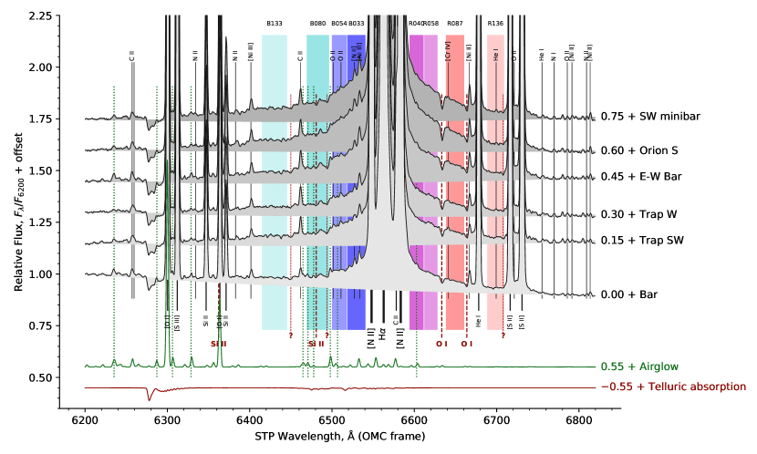
Figure 3: MUSE spectra of the Orion Nebula centered on the H$\alpha$ line, showing the broad Raman-scattered wings. Spectra are shown for the regions outlined by white boxes in Figure 2 and were extracted from the datacubes of Weilbacher et al. (2015). All spectra are normalized to the continuum at $6200\text{\,}\mathrm{\SIUnitSymbolAngstrom}$ and are offset vertically as labelled at right. Emission line identifications are shown by solid vertical lines, labelled above for weak lines and below for stronger lines. Wavelengths of Raman-scattered $\mathrm{O\,\scriptstyle I}$ and $\mathrm{Si\,\scriptstyle II}$ absorption lines from Table 4 are shown by red dashed vertical lines, labelled in bold font below, together with unidentified candidate absorption features marked with “?”. Dotted lines show night sky lines identified in the Dark Bay region of the nebula. At the bottom of the figure are shown the theoretical upper-atmosphere airglow spectrum (green line) and telluric molecular absorption spectrum (red line), as calculated from the Cerro Paranal Advanced Sky Model (Noll et al., 2012; Moehler et al., 2014).

Extended wings to the $\text{H}\alpha$ line are detected over the entire map, but they are particularly prominent in the six regions marked as white boxes in Figure 2(b). These are all bar-like features (O’Dell & Yusef-Zadeh, 2000; García-Díaz & Henney, 2007), which correspond to filamentary ionization fronts. Extracted MUSE spectra around the $\text{H}\alpha$ line for each of these regions are shown in Figure 3. All regions show broad wings to the $\text{H}\alpha$ line extending from $6300$ to $6700\text{\,}\mathrm{\SIUnitSymbolAngstrom}$, which are consistent with the higher spectral resolution ($R=7000$) results of Dopita et al. (2016) for the region indicated by a dashed box in Figure 2(b). The continuum is interpolated under the wings by fitting a second-order polynomial to clean regions of the spectra in the ranges $6070\text{\,}\mathrm{\SIUnitSymbolAngstrom}6225\text{\,}\mathrm{\SIUnitSymbolAngstrom}$ and $6760\text{\,}\mathrm{\SIUnitSymbolAngstrom}6820\text{\,}\mathrm{\SIUnitSymbolAngstrom}$, as shown by the lower edge of the gray shading for each spectrum. The continuum is a combination of Paschen recombination emission from hydrogen, which increases to the red, and dust-scattered starlight and two-photon hydrogen emission, which both increase to the blue. The combined $F_{\lambda}$ is approximately flat for all regions except the Orion Bar, where dust scattering of the nearby star $\theta^{2}\,\text{Ori\leavevmode\nobreak\ A}$ dominates, resulting in a blueward rise. All of these continuum processes are expected to be smooth on a $100\text{\,}\mathrm{\SIUnitSymbolAngstrom}$ scale, but nonetheless the systematic uncertainties in the continuum interpolation is an important factor that limits the precision of the Raman wing measurements.

2.2 Raman scattered FUV absorption lines

A prominent feature of all the spectra in Figure 3 is a pair of absorption notches in the red wing at $6633\text{\,}\mathrm{\SIUnitSymbolAngstrom}$ and $6664\text{\,}\mathrm{\SIUnitSymbolAngstrom}$, which closely correspond to the wavelengths expected for the Raman-scattered transformation of the $\mathrm{O\,\scriptstyle I}$ resonance lines at $1027\text{\,}\mathrm{\SIUnitSymbolAngstrom}$ and $1028\text{\,}\mathrm{\SIUnitSymbolAngstrom}$ listed in Table 4. After correcting for instrumental broadening, the FWHM of the $6633\text{\,}\mathrm{\SIUnitSymbolAngstrom}$ feature is $\approx$2.5\text{\,}\mathrm{\SIUnitSymbolAngstrom}$$, which would correspond to a velocity width of $115\text{\,}\mathrm{k}\mathrm{m}\,\mathrm{s}^{-1}$ if it were an optical absorption line. However, taking into account the wavelength transformation during Raman scattering (eq. [13]), the true velocity width of the FUV line is $18\text{\,}\mathrm{k}\mathrm{m}\,\mathrm{s}^{-1}$. The absorption depth of the features is roughly 50% with respect to the Raman-scattered wing at adjacent wavelengths, but is much less than this with respect to the total continuum emission. The same spectral features are also visible in the Dopita et al. (2016) spectra but are not commented on by those authors. The $6664\text{\,}\mathrm{\SIUnitSymbolAngstrom}$ feature is partially blended with the [$\mathrm{Ni\,\scriptstyle II}$] $6666.8\text{\,}\mathrm{\SIUnitSymbolAngstrom}$ nebular emission line in the MUSE spectra, but these are better resolved in the higher resolution Dopita et al. spectra. Archival Keck HIRES observations of this feature at an even higher spectral resolution are presented below in § 3. The identification of these two FUV absorption lines in the optical spectrum is incontestable proof of a Raman scattering origin for the broad $\text{H}\alpha$ wings.

There is also evidence for a weak absorption feature in the blue wing at $6481\text{\,}\mathrm{\SIUnitSymbolAngstrom}$, corresponding to the $\mathrm{Si\,\scriptstyle II}$ absorption line at $1024\text{\,}\mathrm{\SIUnitSymbolAngstrom}$. However, the blue wing is much less clean than the red wing, partly due to telluric absorption and airglow emission (see below), which makes the identification uncertain. The Raman wings show some other weak features that remain unidentified, the strongest of which is an apparent broad ($\approx$5\text{\,}\mathrm{\SIUnitSymbolAngstrom}$$) absorption feature at $6494\text{\,}\mathrm{\SIUnitSymbolAngstrom}$, while additional narrower features are seen at $6450\text{\,}\mathrm{\SIUnitSymbolAngstrom}$ and $6708\text{\,}\mathrm{\SIUnitSymbolAngstrom}$ (all marked with “?” in Figure 3). It is not clear if these are truly absorption features or whether they are simply gaps between very weak blended emission lines.

2.3 Definition of observational Raman bands in the red and blue wings

Table 1: Wavelength bands used for Raman wing extraction

	Band	$\langle\Delta\lambda_{2}\rangle,$\mathrm{\SIUnitSymbolAngstrom}$$	$\lambda_{\text{min}},$\mathrm{\SIUnitSymbolAngstrom}$$	$\lambda_{\text{max}},$\mathrm{\SIUnitSymbolAngstrom}$$	$f_{\mathrm{H\alpha}}$	$\langle\sigma_{\lambda}\rangle,${10}^{-21}\text{\,}\mathrm{c}\mathrm{m}^{2}$$	Contamination
	(1)	$(2)$	$(3)$	$(4)$	$(5)$	$(6)$	(7)
Blue wing	B133	$-132.8$	$6414.85$	$6445.45$	$0.180$	$0.144$
	B080	$-79.5$	$6469.25$	$6496.45$	$0.196$	$0.378$	Sky 6471, 6478, $\mathrm{H_{2}O}$
	B054	$-53.6$	$6499.85$	$6517.70$	$0.205$	$0.802$	$\mathrm{O\,\scriptstyle II}$? 6502, 6510, Sky 6507, $\mathrm{H_{2}O}$
	B033	$-32.8$	$6518.55$	$6540.65$	$0.212$	$2.069$	[$\mathrm{N\,\scriptstyle II}$] 6527.24, [$\mathrm{Ni\,\scriptstyle III}$] 6533.76, $\mathrm{H_{2}O}$
Red wing	R040	$40.3$	$6594.20$	$6611.20$	$0.238$	$1.451$	Sky 6603
	R058	$57.7$	$6612.05$	$6628.20$	$0.244$	$0.695$
	R087	$87.1$	$6638.40$	$6660.50$	$0.255$	$0.299$	[$\mathrm{Cr\,\scriptstyle IV}$]? 6641
	R136	$135.7$	$6688.55$	$6708.95$	$0.274$	$0.119$	$\mathrm{He\,\scriptstyle I}$ 6699
Columns: (1) Name of band. (2) Mean wavelength displacement from $\text{H}\alpha$ rest wavelength. (3, 4) Upper and lower wavelength limits for the band. (5) Mean value of the $\text{H}\alpha$ branching ratio from virtual $\mathrm{3p}$ levels (see equation [17]). (6) Mean value of $\text{Ly}\beta$ wing cross-section that can feed this band via Raman scattering (see equation [16]). (7) Nebular and telluric lines that may contaminate the band (see text for details).

In order to study the spatial distribution of the Raman-scattered wings, it is convenient to define a series of broad bands on the blue and red sides, which are listed in Table 1 and shown as blue and red shaded vertical stripes in Figure 3. Four bands are defined in each wing, spanning a range in $|\Delta\lambda_{2}|$ from about $30\text{\,}\mathrm{\SIUnitSymbolAngstrom}$ to $150\text{\,}\mathrm{\SIUnitSymbolAngstrom}$. The lower limit of this range is determined by overlap with the strong nebular [$\mathrm{N\,\scriptstyle II}$] emission lines, while the upper limit is due the [$\mathrm{S\,\scriptstyle II}$] lines on the red side, combined with the Raman wings becoming too weak to measure. The mean $\mathrm{H^{0}}$ $\text{Ly}\beta$ cross section corresponding to each band (eq. [16]) is also given in the table, varying between about $1\text{\times}{10}^{-22}\text{\,}\mathrm{c}\mathrm{m}^{2}$ and $2\text{\times}{10}^{-21}\text{\,}\mathrm{c}\mathrm{m}^{2}$.

The bands are chosen so as to avoid the strongest contaminating lines wherever possible, but some small contamination is unavoidable, as listed in the rightmost column of the table. The contamination comes from two sources: weak nebular emission lines (indicated by solid vertical lines in Figure 3) and additionally from the line absorption and emission of the Earth’s atmosphere. Two complementary methods were used to investigate this latter effect. First, the datacube was inspected to identify lines with roughly uniform brightness across the entire map. In particular, any line that is as strong in the Dark Bay region as it is in Orion S is unlikely to come from the nebula itself. Such lines are indicated by vertical dotted lines in Figure 3 and some are listed in Table 1. Second, ESO’s SkyCalc tool was used to predict theoretical emission and absorption spectra for the atmosphere above the VLT at the time and airmass of the observations, convolved with the MUSE instrumental profile. The emission spectrum is dominated by upper-atmosphere airglow lines of $\mathrm{OH}$ (Osterbrock et al., 1996; Noll et al., 2012; Noll et al., 2014), shown in green in the figure, many of which can be seen to coincide with the empirically determined sky lines. The absorption spectrum is dominated by telluric lines of $\mathrm{O_{2}}$ and $\mathrm{H_{2}O}$ (Moehler et al., 2014; Smette et al., 2015). The strongest predicted absorption near $\text{H}\alpha$ is the $\mathrm{O_{2}}$ $\gamma$ band at $6280\text{\,}\mathrm{\SIUnitSymbolAngstrom}$, which is clearly seen in all the spectra, with an absorption depth of order $0.1$, but lies well away from the Raman wings. The blue Raman wing is affected by weaker $\mathrm{H_{2}O}$ bands at $6460\text{\,}\mathrm{\SIUnitSymbolAngstrom}6600\text{\,}\mathrm{\SIUnitSymbolAngstrom}$ with absorption depth $<0.01$, as compared to the relative brightness of the Raman wings at those wavelengths, which is $0.050.1$.

In summary, the nebular and telluric contamination introduces uncertainties of order 10% in the fluxes of the B033, B054, and B080 bands, with other bands being affected to a much lesser degree.

2.4 Spatial distribution of Raman band emission

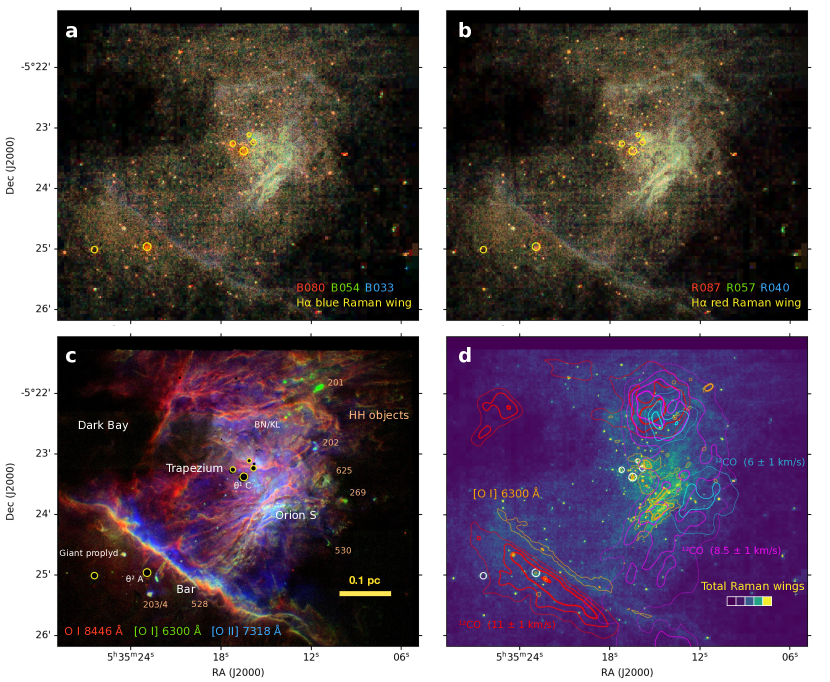
Figure 4: Spatial distribution of Raman-scattered wings of H$\alpha$. (a) Three-color RGB image of bands in the blue wing: B080 (red channel), B054 (green), B033 (blue). All bands are continuum-subtracted and are multibinned at constant signal-to-noise (see text). Maximum brightness in the (red, green, blue) channels is $(2.27,3.89,7.78)\times$1\text{\times}{10}^{-9}\text{\,}\mathrm{e}\mathrm{r}\mathrm{g}\,\mathrm{s}^{-1}\,\mathrm{c}\mathrm{m}^{-2}\,\mathrm{s}\mathrm{r}^{-1}\,\mathrm{\SIUnitSymbolAngstrom}^{-1}$$. The brightest stars are masked out and marked with yellow circles. Lower-mass stars are not masked and most appear as yellow/red dots. (b) Same as (a) but for bands in the red wing: R087 (red), R057 (green), R040 (blue). (c) Three-color RGB image of collisional and fluorescent oxygen emission lines that bracket the ionization front: $\mathrm{O\,\scriptstyle I}$ $\lambda 8446$ (red), [$\mathrm{O\,\scriptstyle I}$] $\lambda 6300$ (green), [$\mathrm{O\,\scriptstyle II}$] $\lambda 7318$ (blue). Various features of the nebula are marked, including Herbig-Haro objects driven by jets from young stars. (d) Comparison of the total Raman wing intensity (blue-to-yellow false color image) with the [$\mathrm{O\,\scriptstyle I}$] emission that traces the ionization front (orange contours) and $\mathrm{{}^{12}CO}$ emission that traces molecular gas (red, purple, and blue contours for different LSR velocities as marked).

Figure 4 shows maps of the six innermost Raman bands as two RGB images: the blue wing in panel a and the red wing in panel b. In each case, the channel sequence R, G, B is an inward progression towards line center, from the farther wings to the nearer wings. The maps are adaptively smoothed following the binary grid algorithm outlined in García-Díaz et al. (2018), which reduces the noise in the fainter regions at the cost of a reduced spatial resolution. The two maps are strikingly similar, indicating that the contamination of the blue wing (see previous section) is indeed a minor effect when integrated over an entire band.

To aid in the interpretation of the Raman wing maps, Figure 4c shows a combined view of mid-to-low-ionization oxygen emission lines, derived from the MUSE data cube. In blue is shown the [$\mathrm{O\,\scriptstyle II}$] $7318.39,$7319.99\text{\,}\mathrm{\SIUnitSymbolAngstrom}$$ doublet, which traces the outer 10% of the fully ionized emission. In green is shown the [$\mathrm{O\,\scriptstyle I}$] $6300.30\text{\,}\mathrm{\SIUnitSymbolAngstrom}$ line, which principally traces partially ionized gas at the ionization front, but also shocks in neutral gas. In red is shown the fluorescent $\mathrm{O\,\scriptstyle I}$ $8446.36\text{\,}\mathrm{\SIUnitSymbolAngstrom}$ line, which traces fully neutral gas that is very close behind the ionization front. This image clearly illustrates that the neutral/molecular gas is organized in filaments, with bright ionization fronts on the side facing the high-mass Trapezium stars. This is most clearly seen in the Orion Bar, the linear emission feature to the south-east of the map, but analogous filaments are seen in all directions from the Trapezium (see also Figure 2b). A particularly complex region, with several partially overlapping filaments, lies between the Trapezium and the Orion S star formation region. This region shows the brightest Raman wing emission, suggesting that it contains the neutral gas with the highest incident FUV flux, presumably because it lies physically closest to the illuminating high-mass stars.

The spatial relation of the Raman-scattered wings to other emission lines is illustrated in Figure 4d, which shows the summed wing intensity over all 8 bands as a false color scale. This is compared with contours that show the ionization front, as traced by the collisionally excited [$\mathrm{O\,\scriptstyle I}$] line, and molecular gas, as traced by the optically thick $\mathrm{{}^{12}CO}$ (1–0) line (Kong et al., 2018). In the Bar region, the Raman emission is clearly seen to be sandwiched between the ionization front and the molecular gas, conclusive evidence that it arises in the neutral zone of the PDR. In the Orion S region and around the Trapezium, there is not such a clear stratification between ionized, neutral, and molecular emission. This is due to two factors: first, the densities are higher, which shortens all length scales, and second, the geometry is not so edge-on, leading to a greater degree of superposition along the line of sight, as witnessed by the overlap of the [$\mathrm{O\,\scriptstyle I}$] and $\mathrm{{}^{12}CO}$ contours. Nonetheless, even here there is evidence that the Raman emission tends to lie farther from $\theta^{1}\,\text{Ori\leavevmode\nobreak\ C}$ than the ionization front, particularly in the “SW minibar” region.

2.5 Emission profiles across the Orion Bar

Figure 5: (a) Spatial cut of continuum-subtracted Raman-scattered H$\alpha$ wing intensity across the Orion Bar. Matched band pairs from the red and blue wings are shown with the same color scheme as in Fig. 3. (b) Comparison with far-infrared observations of line and continuum (purple shading) emission from Herschel PACS (Bernard-Salas et al., 2012). The width (FWHM) of the Herschel PSF is shown by horizontal bars for two representative wavelengths. (c) Comparison with a variety of other tracers of molecular, neutral, and ionized material. Optical lines are from VLT MUSE (Weilbacher et al., 2015), infrared continuum bands (green shading) are from Spitzer IRAC (Megeath et al., 2012), CO lines are from Carma-NRO (Kong et al., 2018) and Herschel PACS (Parikka et al., 2018), $\mathrm{H_{2}}$ near-infrared line is from VLT HAWK-I (Kissler-Patig et al., 2008). (d) Image of the bar in $\mathrm{O\,\scriptstyle I}$, rotated so the $x$ axis is along the direction of the spatial cuts (area indicated by dashed rectangle). Contours of molecular CO emission (red) and ionized [$\mathrm{O\,\scriptstyle III}$] emission (blue) are also shown. In all four panels, ultraviolet photons are incident from the right hand side and the vertical dotted line indicates the ionization front, defined as the peak of the fluorescent $\mathrm{O\,\scriptstyle I}$ emission. The profiles are the median values over a slit width of $75^{\prime\prime}$, centered on the ICRS equatorial coordinates $\alpha=$$$, $\delta=$$$ and oriented at a position angle of $141.5\mathrm{°}$. Distances from the ionization front are given in $\mathrm{m}\mathrm{p}\mathrm{c}$ where $1^{\prime\prime}\approx$1.9\text{\,}\mathrm{m}\mathrm{p}\mathrm{c}$$ for an assumed distance of $388\pm 5\text{\,}\mathrm{p}\mathrm{c}$ (Kounkel et al., 2017).

Table 2: Peaks in emission profiles across the Orion Bar

Emission type and units	Line or Band	$x_{0},$\mathrm{m}\mathrm{p}\mathrm{c}$$	$\delta x,$\mathrm{m}\mathrm{p}\mathrm{c}$$	$I(\text{Peak})$	$I(\text{BG})$	Ref.
(1)	(2)	$(3)$	$(4)$	$(5)$	$(6)$	(7)
$\mathrm{H\,\scriptstyle II}$ region emission lines	[$\mathrm{O\,\scriptstyle III}$] $\lambda 5007$	$-32.1\pm 2.6$	$45$	$13.059$	$11.642\pm 5.605$	1
	[$\mathrm{O\,\scriptstyle II}$] $\lambda 7318$	$-9.4\pm 3.6$	$25$	$0.882$	$0.232\pm 0.026$	1
Peak and BG: $\int I_{\lambda}\,d\lambda$, ${10}^{-6}\text{\,}\mathrm{e}\mathrm{r}\mathrm{g}\,\mathrm{s}^{-1}\,\mathrm{c}\mathrm{m}^{-2}\,\mathrm{s}\mathrm{r}^{-1}$	[$\mathrm{O\,\scriptstyle I}$] $\lambda 6300$	$-1.7\pm 0.1$	$9$	$0.152$	$0.045\pm 0.001$	1
	$\mathrm{O\,\scriptstyle I}$ $\lambda 8446$	$0.0\pm 0.8$	$8$	$0.226$	$0.071\pm 0.000$	2
$\text{H}\alpha$ Raman bands	B033	$0.8\pm 1.5$	$20$	$0.455$	$0.858\pm 0.007$	2
	R040	$1.8\pm 0.1$	$18$	$0.480$	$0.815\pm 0.023$
Peak and BG: $I_{\lambda}$, ${10}^{-9}\text{\,}\mathrm{e}\mathrm{r}\mathrm{g}\,\mathrm{s}^{-1}\,\mathrm{c}\mathrm{m}^{-2}\,\mathrm{s}\mathrm{r}^{-1}\,\mathrm{\SIUnitSymbolAngstrom}^{-1}$	B054	$5.0\pm 2.7$	$9$	$0.233$	$0.641\pm 0.009$
	R058	$5.5\pm 2.8$	$11$	$0.285$	$0.591\pm 0.017$
	B080	$7.1\pm 1.3$	$11$	$0.136$	$0.437\pm 0.013$
	R087	$7.1\pm 0.7$	$15$	$0.178$	$0.393\pm 0.017$
	B133	$6.7\pm 1.1$	$10$	$0.128$	$0.302\pm 0.004$
	R136	$3.1\pm 2.7$	$27$	$0.072$	$0.198\pm 0.007$
Spitzer IRAC bands	$3.6\text{\,}\micron$	$11.6\pm 1.1$	$21$	$0.200$	$0.182\pm 0.018$	3
Peak and BG: $I_{\nu}$, $\mathrm{G}\mathrm{J}\mathrm{y}\,\mathrm{s}\mathrm{r}^{-1}$	$5.8\text{\,}\micron$	$12.8\pm 2.4$	$23$	$1.702$	$0.966\pm 0.073$
	$8.0\text{\,}\micron$	$13.9\pm 3.4$	$24$	$4.866$	$2.622\pm 0.119$
Herschel PACS continuum	$60\text{\,}\micron$	$23.9\pm 7.0$	$52$	$66.361$	$25.175\pm 0.261$	4
Peak and BG: $I_{\nu}$, $\mathrm{J}\mathrm{y}\,\mathrm{p}\mathrm{i}\mathrm{x}^{-1}$	$150\text{\,}\micron$	$39.2\pm 4.2$	$63$	$7.263$	$2.592\pm 0.065$
PDR emission lines	[$\mathrm{N\,\scriptstyle II}$] $122\text{\,}\micron$	$-4.0\pm 1.7$	$55$	$1.907$	$0.581\pm 0.181$	4
	[$\mathrm{O\,\scriptstyle I}$] $63\text{\,}\micron$	$21.6\pm 1.2$	$55$	$1.303$	$0.823\pm 0.242$	4
Peak and BG: $\int I_{\lambda}\,d\lambda$, median normalized	$\mathrm{H_{2}}$ $2.12\text{\,}\micron$	$23.6\pm 0.1$	$19$	$0.169$	$0.997\pm 0.002$	5
	[$\mathrm{C\,\scriptstyle II}$] $158\text{\,}\micron$	$24.3\pm 1.9$	$47$	$0.975$	$0.920\pm 0.145$	4
	[$\mathrm{O\,\scriptstyle I}$] $146\text{\,}\micron$	$26.0\pm 2.8$	$46$	$2.299$	$0.945\pm 0.210$	4
	$\mathrm{{}^{12}CO}$ (19–18)	$33.8\pm 0.1$	$32$	$3.930$	$0.399\pm 0.001$	6
	[$\mathrm{C\,\scriptstyle I}$] $\lambda 8727$	$37.7\pm 5.9$	$30$	$0.495$	$0.854\pm 0.122$	2
	$\mathrm{{}^{12}CO}$ (18–17) $145\text{\,}\micron$	$38.9\pm 0.5$	$34$	$8.193$	$0.989\pm 0.154$	4
	$\mathrm{{}^{12}CO}$ (1–0)	$41.1\pm 1.2$	$44$	$0.472$	$0.746\pm 0.173$	7
	$\mathrm{{}^{13}CO}$ (1–0)	$49.8\pm 2.1$	$33$	$0.891$	$0.823\pm 0.112$	7
Note—Results of fitting a single Gaussian plus linear background to the brightness profiles shown in Figure 5. Columns: (1) Type of tracer and surface brightness units for the values given in columns 5 and 6. (2) Specific emission line or continuum band. (3) Peak position of fitted Gaussian relative to ionization front. Negative values are on the ionized side of the front, positive values on the neutral/molecular side. The uncertainty is determined as the difference between the fitted Gaussian peak and the actual data peak. (4) FWHM of fitted Gaussian. Note that this is not corrected for the instrumental PSF, which contributes at the 10–20% level in the case of the Herschel and CARMA data (references 4 and 7) but is negligible in other cases. (5) Peak intensity of fitted Gaussian, with brightness units given in column 1. (6) Intensity of fitted background at position $x_{0}\pm\delta x$. (7) Data provenance references: 1. VLT–MUSE (Weilbacher et al., 2015); 2. VLT–MUSE (this paper); 3. Spitzer–IRAC (Megeath et al., 2012); 4. Herschel–PACS (Bernard-Salas et al., 2012); 5. VLT–HAWK-I (Kissler-Patig et al., 2008); 6. Herschel–PACS (Parikka et al., 2018); 7. Carma–NRO (Kong et al., 2018).

Figure 5 shows spatial profiles across the Orion Bar of the Raman-scattered bands (panel a), together with other emission lines and bands (panels b and c). In keeping with the dominant tradition in the literature e.g., Fig. 9 of van der Werf et al., 1996, Fig. 2 of Goicoechea et al., 2017, the molecular regions are shown on the left and the ionized regions on the right. The profiles are the median values across a slit of width $75^{\prime\prime}$, as illustrated in Figure 5d. Table 2 shows the positions, widths, and intensities of the peaks in each tracer, as determined by fitting a single Gaussian plus a linear background.

2.5.1 Lines from ionized gas and the ionization front at the Bar

The ionization stratification at the edge of the $\mathrm{H\,\scriptstyle II}$ region is clearly seen in the distribution of the [$\mathrm{O\,\scriptstyle III}$], [$\mathrm{O\,\scriptstyle II}$], [$\mathrm{O\,\scriptstyle I}$], and $\mathrm{O\,\scriptstyle I}$ lines (Fig. 5c). The peak in [$\mathrm{O\,\scriptstyle I}$] emissivity (excited by collisions between electrons and neutral oxygen atoms) is expected to occur at a hydrogen ionization fraction of 50% (Henney et al., 2005), which is displaced by $x_{0}\approx$-1.7\text{\,}\mathrm{m}\mathrm{p}\mathrm{c}$$ from the peak of the $\mathrm{O\,\scriptstyle I}$ fluorescent line. This latter should correspond to an absorption optical depth of approximately unity in the FUV pumping lines, such as those listed in Table 4 see § 5 of Walmsley et al., 2000, corresponding to a neutral hydrogen column density of $N(\mathrm{H^{0}})\approx$1\text{\times}{10}^{19}\text{\,}\mathrm{c}\mathrm{m}^{-2}$$ and therefore an average volume density of $n(\mathrm{H^{0}})=N(\mathrm{H^{0}})/|x_{0}|\approx$2000\text{\,}\mathrm{c}\mathrm{m}^{-3}$$. This value is similar to the peak electron density on the fully ionized side of the ionization front: $n_{e}\approx$3000\text{\,}\mathrm{c}\mathrm{m}^{-3}$$, measured from the [$\mathrm{S\,\scriptstyle II}$] $6717/6731$ ratio (e.g. O’Dell et al., 2017), which occurs at $x\approx$-7\text{\,}\mathrm{m}\mathrm{p}\mathrm{c}$$, close to the peak in the [$\mathrm{O\,\scriptstyle II}$] emission. Therefore, the total hydrogen density is roughly constant over the transition between a predominantly ionized state and predominantly neutral state. Note that the apparent width of this transition (for instance, the FWHM of the [$\mathrm{O\,\scriptstyle I}$] peak $\approx$9\text{\,}\mathrm{m}\mathrm{p}\mathrm{c}$$) is much larger than predicted by atomic physics, which is probably due to spatial irregularities in the ionization front, which can be seen in the inset Figure 5d.

2.5.2 Spatial profiles of the Raman bands in the neutral Bar

Unlike the optical emission lines, the Raman wing bands (upper panel of Fig. 5) all show peaks at positive values of $x$, corresponding to fully neutral gas in the PDR. There is a very close agreement between corresponding pairs of blue and red bands: B033 with R040, B054 with R058, and B080 with R087. However, there is a systematic tendency for the blue band intensity to be slightly higher than its red counterpart on the ionized side (negative values of $x$), which is probably due to contamination by nebular emission lines, as listed in column 7 of Table 1. There is a clear tendency for the peak in the brightness profile to progress towards greater depths into the neutral gas as one moves to wavelengths farther from the $\text{H}\alpha$ line center, which is quantitatively confirmed by the Gaussian fits in Table 2. This result is used as a diagnostic of the PDR density in § 4.2.3 below.

2.5.3 Other PDR tracers of the neutral and molecular Bar

The left hand side of panels b and c of Figure 5 show a variety of other emission lines and continuum bands, which trace different layers in the PDR. The near-infrared $\mathrm{H_{2}}$ $v=1\to 0\ \mathrm{S(1)}$ line marks the hydrogen dissociation front at $x_{0}\approx$24\text{\,}\mathrm{m}\mathrm{p}\mathrm{c}$$ (van der Werf et al., 1996; Luhman et al., 1998; Marconi et al., 1998), which provides the outer boundary of the neutral hydrogen layer. Beyond this are are found the high-$J$ CO lines, which trace the $\mathrm{CO}$ dissociation front at $x_{0}\approx$36\text{\,}\mathrm{m}\mathrm{p}\mathrm{c}$$. These coincide with near-infrared [$\mathrm{C\,\scriptstyle I}$] emission, which mainly traces the recombination of $\mathrm{C^{+}}$ ions in cool gas near the dissociation front (Escalante et al., 1991). The mm-band CO lines trace the deeper, fully molecular regions, with the optically thick $\mathrm{{}^{12}CO\ (1-0)}$ line at $x_{0}\approx$41\text{\,}\mathrm{m}\mathrm{p}\mathrm{c}$$ arising outside of the optically thin $\mathrm{{}^{13}CO\ (1-0)}$ line at $x_{0}\approx$50\text{\,}\mathrm{m}\mathrm{p}\mathrm{c}$$ (Kong et al., 2018).

The broad infrared bands are dominated by dust emission. For the case of the $3.6$ to $8.0\text{\,}\mathrm{\SIUnitSymbolMicro}\mathrm{m}$ Spitzer bands (Megeath et al., 2012), mid-infrared spectroscopy (Bregman et al., 1989; Cesarsky et al., 2000; Kassis et al., 2006) shows that they are mainly due to discrete polycyclic aromatic hydrocarbon (PAH) features at $3.3$, $6.2$, $7.7$, and $8.6\text{\,}\mathrm{\SIUnitSymbolMicro}\mathrm{m}$, plus a continuum contribution from very small grains (VSGs, with size $a\sim$0.007\text{\,}\mathrm{\SIUnitSymbolMicro}\mathrm{m}$$, Desert et al., 1990) and minor contributions from ionized gas lines such as [$\mathrm{Ar\,\scriptstyle II}$] and [$\mathrm{Ar\,\scriptstyle III}$]. The longer wavelength $60$ and $150\text{\,}\mathrm{\SIUnitSymbolMicro}\mathrm{m}$ Herschel bands (Bernard-Salas et al., 2012) show continuum emission from larger grains ($a\sim$0.1\text{\,}\mathrm{\SIUnitSymbolMicro}\mathrm{m}$$). The peak of the dust emission moves deeper into the PDR with increasing wavelength, reflecting the decreasing dust temperature as the stellar radiation field is attenuated (Arab et al., 2012).

A complementary view of the Bar is provided by far-infrared emission lines of neutral and ionized metals observed by Herschel (Bernard-Salas et al., 2012). The [$\mathrm{N\,\scriptstyle II}$] $122\text{\,}\mathrm{\SIUnitSymbolMicro}\mathrm{m}$ line comes from the $\mathrm{H^{+}}$ region and shows a similar distribution to the optical [$\mathrm{O\,\scriptstyle II}$] line. The [$\mathrm{C\,\scriptstyle II}$] $158\text{\,}\mathrm{\SIUnitSymbolMicro}\mathrm{m}$ and [$\mathrm{O\,\scriptstyle I}$] $63$ and $146\text{\,}\mathrm{\SIUnitSymbolMicro}\mathrm{m}$ lines, on the other hand, come from the $\mathrm{H^{0}}$ region of the PDR.

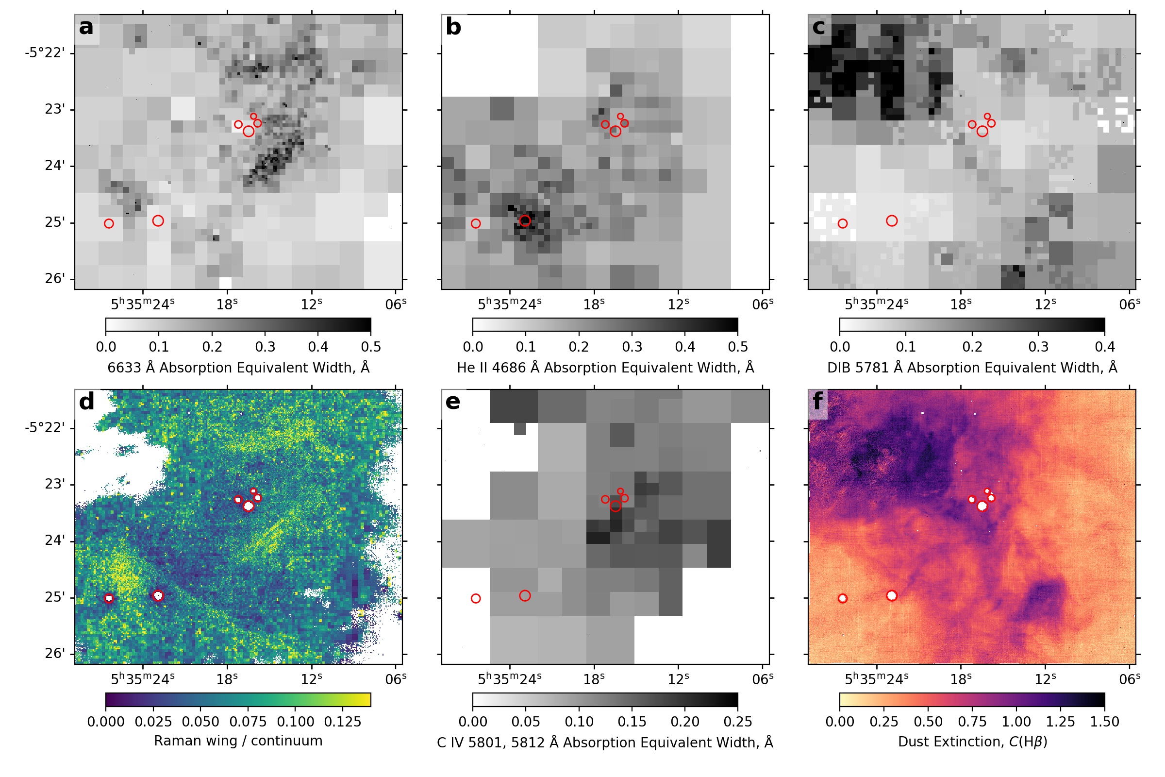
Figure 6: Maps of equivalent widths $W_{\lambda}^{\text{obs}}$ of different absorption features (grayscale images), compared with maps of other quantities (false color images). Red circles show positions of bright stars, from West to East: $\theta^{1}\,\text{Ori\leavevmode\nobreak\ A}$, B, C, D, and $\theta^{2}\,\text{Ori\leavevmode\nobreak\ A}$, B. (a) Equivalent width of $6633\text{\,}\mathrm{\SIUnitSymbolAngstrom}$ absorption feature. (b) Equivalent width of $\mathrm{He\,\scriptstyle II}$ $4685.68\text{\,}\mathrm{\SIUnitSymbolAngstrom}$ absorption line. (c) Equivalent width of a solid-state Diffuse Interstellar Band absorption feature at $5781\text{\,}\mathrm{\SIUnitSymbolAngstrom}$. (d) Ratio $R_{\text{wing}}$ of Raman wing intensity (R058 band) to the intensity of the underlying continuum at the same wavelength. (e) Equivalent width of $\mathrm{C\,\scriptstyle IV}$ $5801.35$, $5811.97\text{\,}\mathrm{\SIUnitSymbolAngstrom}$ absorption line doublet (sum of the two lines). (f) Foreground dust extinction to the ionized gas, $C(\text{H}\beta)$ (base-10 logarithmic extinction at $4861\text{\,}\mathrm{\SIUnitSymbolAngstrom}$), calculated from the Balmer decrement $\text{H}\alpha{}/\text{H}\beta{}$, assuming the reddening curve of Blagrave et al. (2007).

2.6 Equivalent widths of absorption features

Figure 6 shows grayscale maps of the observed equivalent widths, $W_{\lambda}^{\text{obs}}$, of various absorption features that are found superimposed on the continuous spectrum of the Orion Nebula. These are extracted from the MUSE datacubes by integrating over a short wavelength interval, $\Delta\lambda=\pm$8\text{\,}\mathrm{\SIUnitSymbolAngstrom}$$, around the central wavelength of the absorption feature:

$$W_{\lambda}^{\text{obs}}=\int_{\Delta\lambda}\frac{I_{\lambda,\text{cont}}-I_{\lambda}}{I_{\lambda,\text{cont}}}\,d\lambda\quad$\mathrm{\SIUnitSymbolAngstrom}$,$$ (1)

where $I_{\lambda,\text{cont}}$ is the continuum intensity, which is interpolated from the absorption-free portions of the $\Delta\lambda$ interval.

2.6.1 Raman-scattered $\mathrm{O\,\scriptstyle I}$ $1027\text{\,}\mathrm{\SIUnitSymbolAngstrom}$

Figure 6a shows $W_{\lambda}^{\text{obs}}$ for the $6633\text{\,}\mathrm{\SIUnitSymbolAngstrom}$ absorption feature, which is a candidate for being a Raman-scattered FUV absorption line. Note that in this case, the “continuum” intensity $I_{\lambda,\text{cont}}$ includes a contribution from the broad Raman wing, as well as the “true” nebular continuum and dust-scattered starlight. Due to the weakness of both the continuum and the absorption line, it was necessary to aggressively bin the data in order to produce an acceptable map. The results in Figure6d are for a minimum S/N of 7 in $W_{\lambda}^{\text{obs}}$, which gives the optimum balance between noise and spatial resolution.

The 6633 equivalent width is non-zero across the entire map, with a median value of $W_{\lambda}^{\text{obs}}(6633)\approx$0.1\text{\,}\mathrm{\SIUnitSymbolAngstrom}$$. It shows peaks of $W_{\lambda}^{\text{obs}}(6633)=$0.3\pm 0.1\text{\,}\mathrm{\SIUnitSymbolAngstrom}$$ in exactly the same areas as the peaks in the Raman band emission (see § 2.4). For ease of comparison, Figure 6d shows a map of the wing-to-continuum ratio, $R_{\text{wing}}$, for the R087 red Raman wing band, which is found by dividing the continuum-subtracted intensity in the MUSE data cube by the intensity of the interpolated continuum:

$$R_{\text{wing}}=\frac{\int_{\lambda_{\text{min}}}^{\lambda_{\text{max}}}\bigl{(}I_{\lambda}-I^{\prime}_{\lambda,\text{cont}}\bigr{)}\,d\lambda}{\int_{\lambda_{\text{min}}}^{\lambda_{\text{max}}}I^{\prime}_{\lambda,\text{cont}}\,d\lambda},$$ (2)

where the band limits $\lambda_{\text{min}}$, $\lambda_{\text{max}}$ are given in Table 1. In this case, the continuum intensity $I^{\prime}_{\lambda,\text{cont}}$ does not include the Raman wing emission since it is interpolated across a much wider range than in equation (1) by fitting a quadratic function to clean sections of continuum around $6150\pm 80\text{\,}\mathrm{\SIUnitSymbolAngstrom}$ and $6790\pm 30\text{\,}\mathrm{\SIUnitSymbolAngstrom}$ (see § 2.1). Note also that $R_{\text{wing}}$ is a dimensionless ratio, whereas $W_{\lambda}^{\text{obs}}$ has dimensions of wavelength. The reason for choosing the R087 band for this figure is that it is the band that is closest in wavelength to the $6633\text{\,}\mathrm{\SIUnitSymbolAngstrom}$ absorption feature. It is clear from comparing Figure 3 panels a and d that $W_{\lambda}^{\text{obs}}(6633)$ and $R_{\text{wing}}$ closely track one another, as would be expected if the absorption feature is the Raman-scattered $\mathrm{O\,\scriptstyle I}$ $1027\text{\,}\mathrm{\SIUnitSymbolAngstrom}$ line.

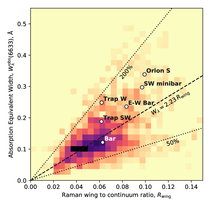
Figure 7: Correlation between $6633\text{\,}\mathrm{\SIUnitSymbolAngstrom}$ equivalent width, $W_{\lambda}^{\text{obs}}(6633)$, and Raman wing to continuum ratio, $R_{\text{wing}}$. False-color image shows histogram of pixels across the face of the nebula, calculated from the MUSE spectral cube: Fig. 6 panel a ($y$ axis) and panel d ($x$ axis). The histogram is weighted by the $6630\text{\,}\mathrm{\SIUnitSymbolAngstrom}$ continuum intensity. The straight dashed line shows the mean relation, $W_{\lambda}=2.27\,R_{\text{wing}}$, while dotted lines show a $2\times$ steeper and $2\times$ shallower slope. Symbols show average values for each of the extraction regions shown by white boxes in Figure 2b.

The relationship is examined more quantitatively in Figure 7, which shows that $W_{\lambda}^{\text{obs}}(6633)$ and $R_{\text{wing}}$ are well-correlated, with a mean slope of $W_{\lambda}=2.27\,R_{\text{wing}}$. Of the six extraction regions used in Figure 3, only the Orion Bar lies on this mean relation. The other regions, which are closer to the Trapezium (see Figure 2b) follow a slope that is roughly 50% steeper. Although this might represent a real physical difference, it is also true that the lower-left area of the graph in Figure 7 is more susceptible to systematic errors. For instance, in the Orion Bar region much of the continuum comes from the blue reflection nebula around $\theta^{2}\,\text{Ori\leavevmode\nobreak\ A}$, which causes increased spectral curvature (see Figure 3), potentially leading to reduced accuracy in the continuum interpolation, which might result in an overestimation of $R_{\text{wing}}$. Higher values of $R_{\text{wing}}$ and $W_{\lambda}$, such as those seen in Orion S, are much less affected by such uncertainties.

2.6.2 Stellar absorption lines

Figure 6b and e show $W_{\lambda}^{\text{obs}}$ for the $\mathrm{He\,\scriptstyle II}$ $4685.68\text{\,}\mathrm{\SIUnitSymbolAngstrom}$ absorption line and the $\mathrm{C\,\scriptstyle IV}$ $5801.35$, $5811.97\text{\,}\mathrm{\SIUnitSymbolAngstrom}$ doublet, respectively. Neither of these lines are expected to be seen in emission from the photoionized gas in the nebula due to the high ionization potentials required. They are therefore well-suited for tracing the diffuse dust-scattered starlight in the nebula. It can be seen that the distribution of the two lines is very different. For the $\mathrm{He\,\scriptstyle II}$ line, one finds $W_{\lambda}^{\text{obs}}(4686)\approx$0.2\text{\,}\mathrm{\SIUnitSymbolAngstrom}$$ across most of the nebula, but with consistently larger values to the SE, with a pronounced peak of $W_{\lambda}^{\text{obs}}(4686)=$0.4\pm 0.1\text{\,}\mathrm{\SIUnitSymbolAngstrom}$$ around the star $\theta^{2}\,\text{Ori\leavevmode\nobreak\ A}$. In addition, there is a secondary peak of $W_{\lambda}^{\text{obs}}(4686)=$0.3\pm 0.05\text{\,}\mathrm{\SIUnitSymbolAngstrom}$$, located close to $\theta^{1}\,\text{Ori\leavevmode\nobreak\ D}$, the easternmost of the four Trapezium stars. In contrast, the $\mathrm{C\,\scriptstyle IV}$ lines show a broad maximum of $W_{\lambda}^{\text{obs}}(5801+5812)=$0.16\pm 0.04\text{\,}\mathrm{\SIUnitSymbolAngstrom}$$, centered to the SW of the Trapezium.

The most straightforward of these to interpret is $\mathrm{C\,\scriptstyle IV}$, since the 5801,5812 doublet is present in the spectrum of $\theta^{1}\,\text{Ori\leavevmode\nobreak\ C}$, with a summed equivalent width $W_{\lambda}^{\star}=$0.44\pm 0.04\text{\,}\mathrm{\SIUnitSymbolAngstrom}$$ (Stahl et al., 1996), but is absent in all the other OB stars in the nebula (as measured from the MUSE datacube). The equivalent width observed in the nebula is smaller than this, because of dilution by the nebular continuum (recombination plus 2-photon) and the starlight from the lower mass members of the Trapezium cluster. The fraction of the total observed continuum intensity that is due to dust-scattering of $\theta^{1}\,\text{Ori\leavevmode\nobreak\ C}$ can be estimated as $f_{\text{scat}}=W_{\lambda}^{\text{obs}}/W_{\lambda}^{\star}$, for which we find a maximum value of $f_{\text{scat}}(\theta^{1}\,\text{Ori\leavevmode\nobreak\ C};\,\mathrm{C\,\scriptstyle IV})=0.4\pm 0.1$ in the region between the Trapezium and Orion S.

Although $\theta^{1}\,\text{Ori\leavevmode\nobreak\ C}$ (spectral type O7V f?p var; Simón-Díaz et al., 2006; Maíz Apellániz et al., 2019) is the hottest and most luminous star in the nebula, its $\mathrm{He\,\scriptstyle II}$ 4686 absorption line is anomalously weak and varies markedly on a rotational timescale of $15.4\text{\,}\mathrm{d}\mathrm{a}\mathrm{y}\mathrm{s}$ (Conti, 1972; Stahl et al., 1993) because it is partially filled in by emission from the magnetosphere and complex magnetically-channeled stellar wind (Donati et al., 2002). From Fig. 5 of Stahl et al. (1996), it can be seen that $W_{\lambda}^{\star}(\theta^{1}\,\text{Ori\leavevmode\nobreak\ C};\,4686)$ varies systematically from $-0.1\text{\,}\mathrm{\SIUnitSymbolAngstrom}$ to $0.4\text{\,}\mathrm{\SIUnitSymbolAngstrom}$ as a function of rotational phase. Three-dimensional simulations (ud-Doula et al., 2013) show that the line profile is dominated by emission ($W_{\lambda}^{\star}<0$) for viewing directions along the magnetic pole, but by photospheric absorption ($W_{\lambda}^{\star}>0$) for viewing directions in the magnetic equator. Comparison with observed phase-dependent line profiles suggests that both the line-of-sight from Earth and the magnetic dipole axis are inclined at $\approx$$$ from the rotation axis. This implies that the spectrum seen from Earth, integrated over the rotational period, is broadly representative of the average stellar spectrum seen by the surrounding nebula, so that a value of $W_{\lambda}^{\star}(\theta^{1}\,\text{Ori\leavevmode\nobreak\ C};\,4686)\approx$0.15\text{\,}\mathrm{\SIUnitSymbolAngstrom}$$ is appropriate, albeit with a large uncertainty.

The second most luminous star in the nebula is the spectroscopic binary $\theta^{2}\,\text{Ori\leavevmode\nobreak\ A}$ (spectral type O9.2V + B0.5:V(n); Maíz Apellániz et al., 2019), located to the SE of the nebula, beyond the Bright Bar. This shows a much simpler $\mathrm{He\,\scriptstyle II}$ line profile with $W_{\lambda}^{\star}(\theta^{2}\,\text{Ori\leavevmode\nobreak\ A};\,4686)=$0.53\text{\,}\mathrm{\SIUnitSymbolAngstrom}$$ (Simón-Díaz et al., 2006), which explains why $W_{\lambda}^{\text{obs}}(4686)$ is higher around $\theta^{2}\,\text{Ori\leavevmode\nobreak\ A}$, than around the Trapezium. Applying the same argument as above yields a maximum value of $f_{\text{scat}}(\theta^{2}\,\text{Ori\leavevmode\nobreak\ A};\,\mathrm{He\,\scriptstyle II})=0.75\pm 0.2$, implying that the blue continuum in this area of the nebula is totally dominated by scattered light from $\theta^{2}\,\text{Ori\leavevmode\nobreak\ A}$, which forms a roughly circular reflection nebula.

The same absorption line is present in the spectra of other Trapezium stars, being strongest in the B0.5V star $\theta^{1}\,\text{Ori\leavevmode\nobreak\ D}$ with $W_{\lambda}^{\star}(\theta^{1}\,\text{Ori\leavevmode\nobreak\ D};\,4686)\approx$0.25\text{\,}\mathrm{\SIUnitSymbolAngstrom}$$ (Simón-Díaz et al., 2006). It is therefore interesting and suggestive that the local peak in $W_{\lambda}^{\text{obs}}(4686)$ is on $\theta^{1}\,\text{Ori\leavevmode\nobreak\ D}$’s side of the Trapezium. This would not be expected if all the Trapezium stars lay at the same distance from the scattering grains because $\theta^{1}\,\text{Ori\leavevmode\nobreak\ C}$ is 4 times brighter than $\theta^{1}\,\text{Ori\leavevmode\nobreak\ D}$ at visual wavelengths, so the latter star contributes relatively little to the total luminosity of the Trapezium. However, it has been suggested (Smith et al., 2005) that $\theta^{1}\,\text{Ori\leavevmode\nobreak\ D}$ may lie closer to the background molecular gas, roughly $0.1\text{\,}\mathrm{p}\mathrm{c}$ behind $\theta^{1}\,\text{Ori\leavevmode\nobreak\ C}$. In such a case, it would be possible for $\theta^{1}\,\text{Ori\leavevmode\nobreak\ D}$ to dominate the illumination of a small reflection nebula around itself, and the present results would tend to confirm that.

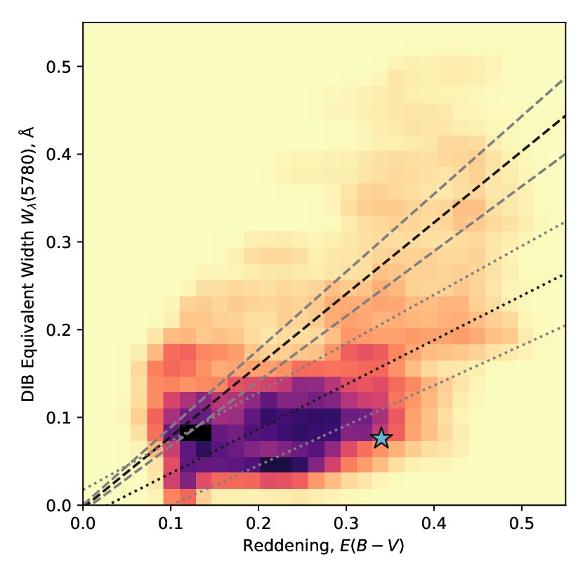
Figure 8: Correlation between DIB equivalent width, $W_{\lambda}^{\text{obs}}(5780)$, and reddening, $E(B-V)$. False-color image shows histogram of pixels across the face of the nebula, calculated from the MUSE spectral cube: Fig. 6 panel c ($y$ axis) and panel f ($x$ axis), assuming $E(B-V)=0.3845\,C(\text{H}\beta)$. Straight lines shows fits to surveys of DIBs along $\sigma$-type sight lines to stars (dotted line, Kos & Zwitter, 2013) and high-Galactic-latitude sight lines to external galaxies (dashed line, Baron et al., 2015). Star symbol shows result for $\theta^{1}\,\text{Ori\leavevmode\nobreak\ C}$ (Friedman et al., 2011).

2.6.3 Solid-state absorption features

A third type of absorption feature found in the nebular spectrum is what is known as Diffuse Interstellar Bands (DIBs; Heger, 1922), of which hundreds are now known (Galazutdinov et al., 2000; Hobbs et al., 2008). The majority are believed to be due to large carbon-based molecules associated with atomic gas (Sonnentrucker, 2014) but, apart from in a few instances (Cordiner et al., 2019), their exact nature is still uncertain (Tielens, 2014; Omont et al., 2019; Lai et al., 2020). The strongest such feature found in the MUSE spectra is the well-known band at $5780\text{\,}\mathrm{\SIUnitSymbolAngstrom}$, which is shown in Figure 6c. For comparison, the foreground extinction to the nebula is shown in Figure 6f, which is calculated from the $\text{H}\alpha$/$\text{H}\beta$ ratio, assuming the extinction curve of Blagrave et al. (2007).

It is clear at a glance that the spatial distribution of the DIB absorption and the continuum dust absorption are very similar. This is not surprising, since many studies have established a correlation between DIB equivalent widths and interstellar reddening (Friedman et al., 2011; Kos & Zwitter, 2013; Baron et al., 2015; Krełowski et al., 2019). This is tested quantitatively in Figure 8, which shows the correlation between $W_{\lambda}^{\text{obs}}(5780)$ and dust reddening $E(B-V)$. The relative weakness of the $5797\text{\,}\mathrm{\SIUnitSymbolAngstrom}$ DIB feature in all Orion Nebula sight lines is characteristic of $\sigma$-type DIBS (after the prototype $\sigma$ Sco; Krełowski & Westerlund, 1988), which tend to be found in atomic diffuse clouds. I therefore compare the results with a fit to 27 $\sigma$-type sight lines to OB stars from the survey of Kos & Zwitter (2013) (dotted line in Figure 8), which covers the reddening range $E(B-V)=0.1$ to $1.2$. I also show (dashed line in figure) a fit to over a million stacked external galaxy and quasar sight lines from SDSS (Baron et al., 2015), which cover the reddening range $E(B-V)=0$ to $0.11$. It can be seen that the nebular values follow the general trend of the fits, albeit with considerable dispersion. The tail of high $W_{\lambda}$ above the fit lines may be due to the fact that a significant fraction of the continuum is dust-scattered and those photons will have traversed a larger column of dust than is measured by the foreground reddening. In addition, the Balmer decrement will saturate at high column densities if part of the dust is mixed with the emitting gas, resulting in an underestimate of $E(B-V)$.

A further DIB feature is seen in the spectra at $6284\text{\,}\mathrm{\SIUnitSymbolAngstrom}$. However, it is hard to estimate the equivalent width of this feature since it overlaps with telluric $\mathrm{O_{2}}$ $\gamma$-band absorption (see Figure 3).

3 High-resolution spectroscopy of Raman-scattered $\mathrm{O\,\scriptstyle I}$ $1028\text{\,}\mathrm{\SIUnitSymbolAngstrom}$

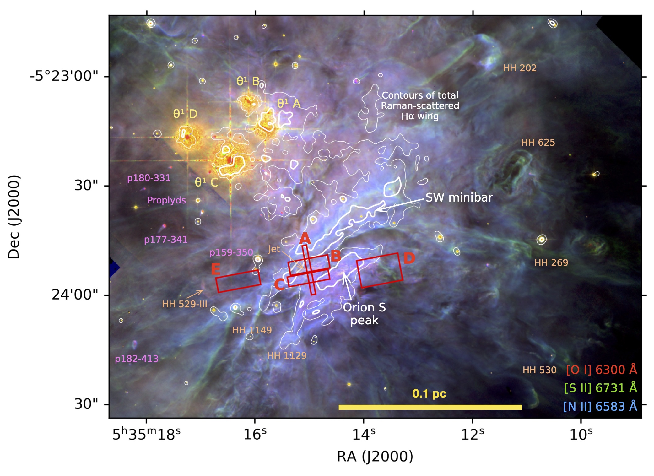
Figure 9: Zoom on Trapezium and Orion South region, showing the locations of extracted Keck spectra (red boxes). The background color composite image shows HST WFPC2 observations in the filters F631N, F673N, and F658N (Bally et al., 2000), which highlight emission from the ionization front and adjacent regions. White contours show the total Raman-scattered $\text{H}\alpha$ wing emission (sum of the six wavelength bands listed in Table 1).

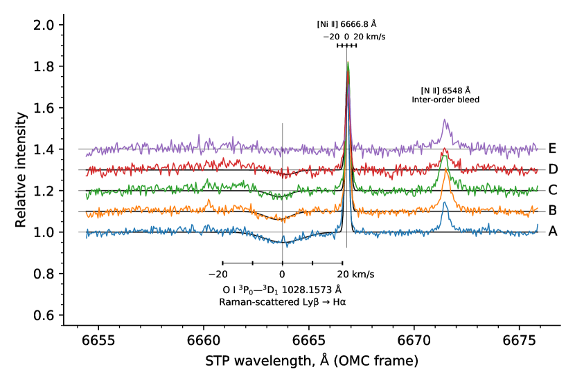
Figure 10: Continuum-normalized Keck HIRES spectra of Raman-scattered $\mathrm{O\,\scriptstyle I}$ absorption line for five regions in Orion South. Spectra are offset vertically for ease of comparison. The location of each region is given in Figure 9. Wavelengths are given on an air scale and in the rest-frame of the Orion Molecular Cloud, as defined by the peak velocity of $\mathrm{{}^{13}CO}$. Black continuous lines show single-Gaussian fits to the $\mathrm{O\,\scriptstyle I}$ absorption line and adjacent [$\mathrm{Ni\,\scriptstyle II}$] emission line, with fit parameters given in Table 3.

In order to obtain observations of the Raman-scattered $\mathrm{O\,\scriptstyle I}$ absorption lines at high spectral resolution, I have searched through archival spectra of the Orion Nebula obtained with the HIRES spectrograph on the Keck I telescope (Vogt et al., 1994). The observations, obtained in 1997 December 5 and 6, were targeted at a small number of proplyds and jets in the nebula and are described in detail in Henney & O’Dell (1999) and Bally et al. (2000). Unfortunately, the stronger $6633\text{\,}\mathrm{\SIUnitSymbolAngstrom}$ feature falls in a gap between adjacent spectrograph orders and so was not observed. However, the weaker $6664\text{\,}\mathrm{\SIUnitSymbolAngstrom}$ feature falls in order 53 and is detected in many of the spectra. Results for the proplyds will be presented elsewhere, and I concentrate here on 16 slit positions located in the Orion South region, roughly $30\text{\,}\mathrm{a}\mathrm{r}\mathrm{c}\mathrm{s}\mathrm{e}\mathrm{c}$ SW of the Trapezium. Closely similar slit positions are co-added to improve S/N, forming five groups, A to E, with positions shown in Figure 9. Most of the slits are $28\text{\,}\mathrm{a}\mathrm{r}\mathrm{c}\mathrm{s}\mathrm{e}\mathrm{c}$ long and $0.574\text{\,}\mathrm{a}\mathrm{r}\mathrm{c}\mathrm{s}\mathrm{e}\mathrm{c}$ wide, but only the central $11\text{\,}\mathrm{a}\mathrm{r}\mathrm{c}\mathrm{s}\mathrm{e}\mathrm{c}$ of order 53 is usable for faint lines due to overlap of adjacent orders.

The broad Raman-scattered wings to $\text{H}\alpha$ are spread over several spectrograph orders and uncertainties in the flat-field correction means that it is impossible to separate the wings from the nebular continuum. Therefore, I simply fit a 5th-order polynomial to line-free sections of the spectrum over the entire order ($6649\text{\,}\mathrm{\SIUnitSymbolAngstrom}$ to $6747\text{\,}\mathrm{\SIUnitSymbolAngstrom}$) and divide to give a continuum-normalized spectrum. Results for the four groups are shown in Figure 10 for the wavelength range of interest. A shallow broad absorption feature is clearly seen around $6664\text{\,}\mathrm{\SIUnitSymbolAngstrom}$ in regions A, B, and C, and arguably in region D, while no such feature is seen in region E. At this high spectral resolution (resolving power $R\approx$50\,000$$), the absorption line is well-separated from the adjacent [$\mathrm{Ni\,\scriptstyle II}$] emission line at $6666.8\text{\,}\mathrm{\SIUnitSymbolAngstrom}$. From Figure 9 it can be seen that regions A, B, and C overlap with contours of strong $\text{H}\alpha$ wing emission in the SW minibar, while region E lies in a higher ionization part of the nebula, where the $\text{H}\alpha$ wing is weak. This is consistent with the observed relative absorption depths, assuming that the $6664\text{\,}\mathrm{\SIUnitSymbolAngstrom}$ feature is due to Raman scattering of the $\mathrm{O\,\scriptstyle I}$ $1028.157\,29\text{\,}\mathrm{l}$ine (see Table 4).

Table 3: Parameters from single-Gaussian line fits to Keck HIRES spectra

Region	$\text{Relative amplitude},\ A$	$V,\ $\mathrm{k}\mathrm{m}\,\mathrm{s}^{-1}$$	$\Delta V,\ $\mathrm{k}\mathrm{m}\,\mathrm{s}^{-1}$$
(1)	$(2)$	$(3)$	$(4)$
	[$\mathrm{Ni\,\scriptstyle II}$] emission $6666.80\text{\,}\mathrm{\SIUnitSymbolAngstrom}$
A	$0.75\pm 0.02$	$0.4\pm 0.1$	$7.7\pm 0.4$
B	$0.71\pm 0.02$	$2.7\pm 0.1$	$7.9\pm 0.4$
C	$0.60\pm 0.02$	$2.9\pm 0.2$	$8.6\pm 0.5$
D	$0.46\pm 0.01$	$1.8\pm 0.2$	$8.5\pm 0.4$
E	$0.29\pm 0.01$	$3.6\pm 0.2$	$6.8\pm 0.6$
	$\mathrm{O\,\scriptstyle I}$ Raman-scattered absorption $6663.75\text{\,}\mathrm{\SIUnitSymbolAngstrom}$
A	$0.050\pm 0.003$	$0.3\pm 0.4$	$14.5\pm 1.0$
B	$0.039\pm 0.004$	$-1.6\pm 0.5$	$9.6\pm 1.1$
C	$0.030\pm 0.005$	$-1.2\pm 0.6$	$7.6\pm 1.5$
D	$0.022\pm 0.007$	$1.3\pm 1.0$	$7.2\pm 2.5$
Columns: (1) Region of nebula covered by HIRES slits (see Figure 9). (2) Peak emission height or absorption depth relative to continuum. (3) Centroid velocity in frame of molecular cloud. (4) Intrinsic full-width half-maximum line width, after correction for the instrumental width of $6\text{\,}\mathrm{k}\mathrm{m}\,\mathrm{s}^{-1}$. Note that in the case of the $\mathrm{O\,\scriptstyle I}$ Raman-scattered absorption line the centroid velocity and line widths have been divided by $6.4$ to account for the stretching of the Doppler scale between the UV and optical frames.

Table 3 shows results for each slit from fitting both the $\mathrm{O\,\scriptstyle I}$ absorption line and the [$\mathrm{Ni\,\scriptstyle II}$] emission line. A single Gaussian component is used for each line and the fits are performed with the astropy.modeling package. The $\mathrm{O\,\scriptstyle I}$ ultraviolet rest wavelength and its optical counterpart after Raman scattering are discussed in Appendix A, while the [$\mathrm{Ni\,\scriptstyle II}$] rest wavelength comes from hollow cathode tube observations Shenstone (1970). Velocities are given in the reference frame of molecular gas in the Orion South region, as defined by the centroid of $\mathrm{{}^{13}CO}$ emission (Kong et al., 2018): $V_{\mathrm{LSR}}=$+9.0\pm 0.2\text{\,}\mathrm{k}\mathrm{m}\,\mathrm{s}^{-1}$$ or $V_{\odot}=$+28.1\pm 0.2\text{\,}\mathrm{k}\mathrm{m}\,\mathrm{s}^{-1}$$. Both the emission and absorption lines have velocities that are close to that of the molecular gas, as has been previously found for low-ionization lines in the nebula e.g., Fig. 14 of Baldwin et al., 2000.

The line width is of order $8\text{\,}\mathrm{k}\mathrm{m}\,\mathrm{s}^{-1}$ for [$\mathrm{Ni\,\scriptstyle II}$], which is predominantly non-thermal since the thermal broadening is only $3\text{\,}\mathrm{k}\mathrm{m}\,\mathrm{s}^{-1}$ for $T=${10}^{4}\text{\,}\mathrm{K}$$. Compared with other optical emission lines that form near the ionization front, the [$\mathrm{Ni\,\scriptstyle II}$] width is intermediate between the widths of fluorescent lines (e.g., [$\mathrm{N\,\scriptstyle I}$]: $6\pm 3\text{\,}\mathrm{k}\mathrm{m}\,\mathrm{s}^{-1}$ Ferland et al., 2012) and collisionally excited lines (e.g., [$\mathrm{O\,\scriptstyle I}$]: $11.5\pm 2.6\text{\,}\mathrm{k}\mathrm{m}\,\mathrm{s}^{-1}$ García-Díaz et al., 2008). The Raman-scattered $\mathrm{O\,\scriptstyle I}$ line shows the greatest width ($W\approx$15\text{\,}\mathrm{k}\mathrm{m}\,\mathrm{s}^{-1}$$) in region A, which is where the absorption is strongest, but is significantly narrower ($W=$7$$ to $10\text{\,}\mathrm{k}\mathrm{m}\,\mathrm{s}^{-1}$) in the other regions.

In principle, the kinematics of Raman-scattered lines should be measurable to a higher precision than that of regular lines. This is because the stretching of the Doppler scale means that the effective spectrograph resolving power is multiplied by $6.4$ to become $R^{\prime}=$320\,000$$. However, as can be seen from Table 3, the precision of the centroid velocity and width measurements is actually lower for $\mathrm{O\,\scriptstyle I}$ than for [$\mathrm{Ni\,\scriptstyle II}$]. This is entirely due of the lower signal-to-noise of the absorption line measurements. Therefore, much longer total exposure times than the $4\times$300\text{\,}\mathrm{s}$$ of the slits that contribute to region A would be necessary to take full advantage of the boost in spectral resolution provided by Raman scattering.

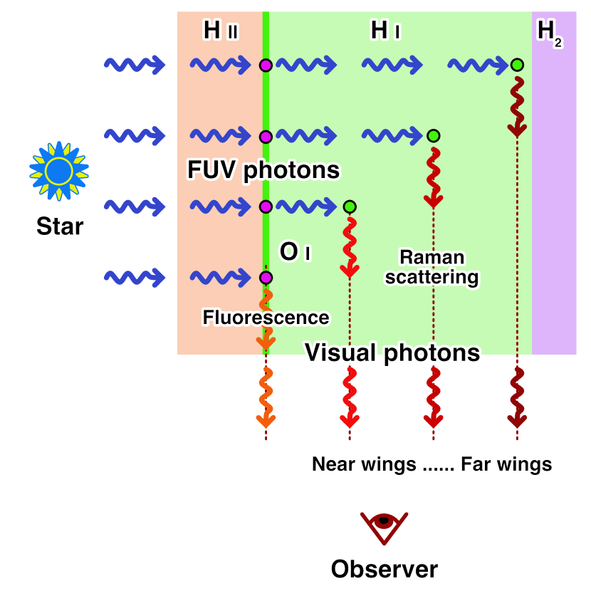
Figure 11: Simplified schematic of where Raman scattering occurs in a PDR. Stellar far-ultraviolet photons (blue wavy arrows) that are far-removed in wavelength from resonant $\mathrm{H\,\scriptstyle I}$ lines can pass through the photoionized $\mathrm{H\,\scriptstyle II}$ layer relatively unscathed. Some of them will be absorbed by metal resonance lines, such as $\mathrm{O\,\scriptstyle I}$ (magenta circles) close to the ionization front, and fluorescently converted to visual/IR photons (orange wavy arrows). This produces a spectral imprint of the $\mathrm{O\,\scriptstyle I}$ absorption on the FUV photons that propagate into the PDR. Once the FUV photons have traversed a sufficient column, they will be non-resonantly scattered by $\mathrm{H\,\scriptstyle I}$ (green circles) and a significant fraction will be Raman-converted to visual photons (red wavy arrows). For wavelengths farther from line center, this Raman scattering occurs deeper in the PDR and is eventually limited by competition from dust absorption and/or the finite total $\mathrm{H\,\scriptstyle I}$ column.

4 Discussion

In this section, I provide a provisional interpretation of the observational evidence from sections 2 and 3 in the light of simple heuristic models of Raman scattering, such as is illustrated schematically in Figure 11. In section 4.1 I present some formal results from radiative transfer theory that will be used in the following discussion. Section 4.2 investigates how the spatial and spectral characteristics of the broad $\text{H}\alpha$ wings can be used to diagnose the physical conditions in the PDR. Section 4.3 considers what extra information can be obtained from the narrow absorption features that are superimposed on the Raman-scattered wings.

4.1 Raman radiative transfer

The Raman scattering process can be divided conceptually into three steps. In step 1, radiative transfer in the FUV band determines the FUV mean intensity, $J_{\lambda}(\lambda_{1})$, at some point in the nebula. In step 2, the scattering itself (see Appendix A) determines a visual-band emission coefficient $j_{\lambda}(\lambda_{2})$ that is proportional to $J_{\lambda}(\lambda_{1})$, where the visual wavelength, $\lambda_{2}$, and FUV wavelength, $\lambda_{1}$, are related by equation (13). In step 3, radiative transfer in the visual band determines the observed intensity of the $\text{H}\alpha$ wing, $I_{\lambda}(\lambda_{2})$. I now consider each of these in turn.

If the FUV radiation field at a point is dominated by a single star of luminosity $L_{\lambda}^{*}(\lambda_{1})$ at a distance $R$, then for step 1 we may write

$$4\pi J_{\lambda}(\lambda_{1})=\frac{L_{\lambda}^{*}(\lambda_{1})}{4\pi R^{2}}\,e^{-\tau_{1}}\quad$\mathrm{e}\mathrm{r}\mathrm{g}\,\mathrm{s}^{-1}\,\mathrm{c}\mathrm{m}^{-2}\,\mathrm{\SIUnitSymbolAngstrom}^{-1}$$$ (3)

where $\tau_{1}$ is the FUV optical depth between the point and the star:

$$\tau_{1}=\int_{0}^{R}k_{\text{total}}(\lambda_{1})\,dR^{\prime}.$$ (4)

The total FUV extinction coefficient can be written as a sum over all absorbing species:

$$k_{\text{total}}(\lambda_{1})=\sum_{i}n_{i}\sigma_{i}(\lambda_{1})\quad$\mathrm{c}\mathrm{m}^{-1}$$$ (5)

Potentially important broad-band absorbers are dust grains and the $\mathrm{H^{0}}$ Rayleigh/Raman scattering itself. Resonance lines of ions, atoms, and molecules may also be important over narrow ranges of $\lambda_{1}$. More realistically, one would sum over several equations like equation (3) for the different stars, and also include the diffuse field due to recombinations, Rayleigh scattering, and dust scattering.

For step 2, assuming that the scattering is isotropic, the visual-band emission coefficient is simply

$$j_{\lambda}(\lambda_{2})=\left(\frac{\lambda_{1}}{\lambda_{2}}\right)^{3}J_{\lambda}(\lambda_{1})\,n(\mathrm{H^{0}})\,\sigma(\lambda_{1})\,f_{\text{H}\alpha}(\lambda_{1})\\ $\mathrm{e}\mathrm{r}\mathrm{g}\,\mathrm{s}^{-1}\,\mathrm{c}\mathrm{m}^{-3}\,\mathrm{s}\mathrm{r}^{-1}\,\mathrm{\SIUnitSymbolAngstrom}^{-1}$,$$ (6)

where $n(\mathrm{H^{0}})$ is the number density of neutral hydrogen atoms, $\sigma(\lambda_{1})$ is the Rayleigh scattering cross section in the $\text{Ly}\beta$ wing given by equation (16), and $f_{\text{H}\alpha}$ is the branching ratio for Raman conversion given by equation (17). The factor $(\lambda_{1}/\lambda_{2})^{3}$ includes one power of $\lambda_{1}/\lambda_{2}$ to account for the reduction in energy per photon when passing from the FUV to visual bands, plus two powers of $\lambda_{1}/\lambda_{2}$ to account for the transformation of per-angstrom, $d/d\lambda_{1}\to d/d\lambda_{2}$.

For step 3, the observable intensity, as shown in Figures 4ab and 5a, is given by an integral over all scattering points $z$ along the line of sight (los):

$$I_{\lambda}(\lambda_{2})=\int_{\text{los}}j_{\lambda}(\lambda_{2})\,e^{-\tau_{2}(z)}\,dz\quad$\mathrm{e}\mathrm{r}\mathrm{g}\,\mathrm{s}^{-1}\,\mathrm{c}\mathrm{m}^{-2}\,\mathrm{s}\mathrm{r}^{-1}\,\mathrm{\SIUnitSymbolAngstrom}^{-1}$,$$ (7)

where $\tau_{2}$ is the visual-band optical depth between each point $z$ and the observer:

$$\tau_{2}(z)=\int_{0}^{z}k_{\text{total}}(\lambda_{2})\,dz^{\prime}$$ (8)

Similarly to the FUV case, the visual-band extinction coefficient $k_{\text{total}}(\lambda_{2})$ can be written as a sum over absorbing species, but the only significant absorber in this case is dust.

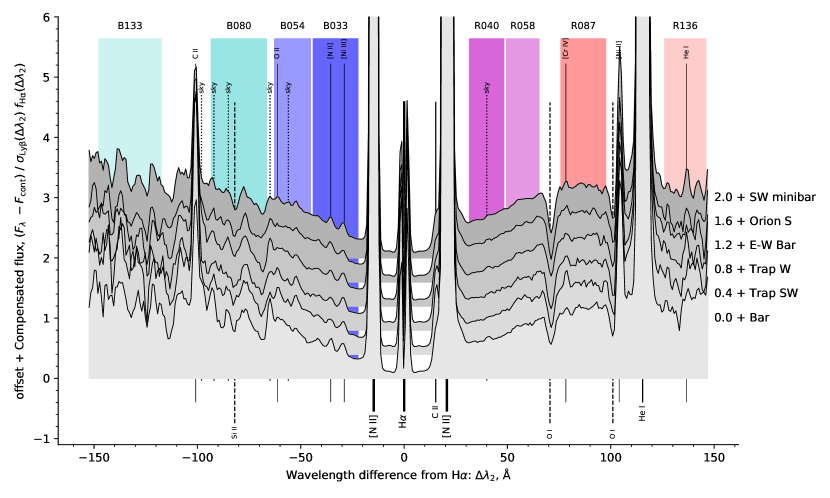
Figure 12: Same as Fig. 3 but with $F_{\lambda}$ divided by the effective cross section to Raman scattering $\sigma\,f_{\text{H}\alpha}$ (see Appendix A) and zoomed in on the Raman wing wavelengths. The spectrum is normalized by the average flux in the R087 band and each region is offset vertically by a constant value, as indicated at right. In this presentation, optically thin Raman scattering of a flat FUV spectrum should give a constant value, which for the Orion data is only seen in the R087 and R136 bands.

4.2 Broad-band Raman scattering

An important question to answer with the Raman scattering is whether it is optically thick or optically thin. There are two optical paths to consider (see previous section): the pre-scattered $\tau_{1}$ of the FUV photons and the post-scattered $\tau_{2}$ of the visual-band photons. Of these, it is $\tau_{1}$ that is most interesting since it is affected not only by dust extinction, but also by the opacity of the Rayleigh/Raman scattering itself. The cross section of the $\text{Ly}\beta$ wings varies by more than an order of magnitude between the different Raman bands (column 6 of Table 1), so it is possible that the nearer wings may be optically thick, while the farther wings are optically thin.

4.2.1 Optically thin limit

For the totally optically thin case, $\tau_{1},\tau_{2}\ll 1$, equations (3, 6, and 7) can be combined to yield

$$I_{\lambda}(\lambda_{2})\approx\left(\frac{\lambda_{1}}{\lambda_{2}}\right)^{3}\,\sigma(\lambda_{1})\,f_{\text{H}\alpha}(\lambda_{1})\,\frac{L_{\lambda}^{*}(\lambda_{1})}{16\pi^{2}}\int_{\text{los}}\frac{n(\mathrm{H^{0}})}{R^{2}}\,dz\\ $\mathrm{e}\mathrm{r}\mathrm{g}\,\mathrm{s}^{-1}\,\mathrm{c}\mathrm{m}^{-2}\,\mathrm{s}\mathrm{r}^{-1}\,\mathrm{\SIUnitSymbolAngstrom}^{-1}$.$$ (9)

When considering the ratio of Raman-scattered intensities between two different wavelengths for the same position on the nebula, then the line-of-sight integral cancels and one finds

$$\frac{I_{\lambda}(\lambda_{2})}{\sigma(\lambda_{1})\,f_{\text{H}\alpha}(\lambda_{1})}\propto L_{\lambda}^{*}(\lambda_{1}).$$ (10)

The left-hand side of this equation (approximately $(\Delta\lambda_{2})^{2}\,I_{\lambda}(\lambda_{2})$) is plotted in Figure 12 for the same extraction regions as in Figure 3. For parts of the spectrum where the scattering is optically thin, this should be proportional to the incident FUV spectrum, $L_{\lambda}^{*}(\lambda_{1})$, which is dominated by the Trapezium OB stars.

It can be seen that the red wing of this compensated spectrum shows an approximately flat section between $+80$ and $+150\text{\,}\mathrm{\SIUnitSymbolAngstrom}$ from $\text{H}\alpha$, covering the R087 and R136 Raman bands. This is consistent with optically thin scattering of a flat FUV spectrum at these wavelengths. However, the behavior is not so clear-cut in the blue wing, where the compensated spectrum continues rising away from line center. Although the slope is slightly shallower in the farther wing (B080 and B133 bands), it never becomes as clearly flat as on the red side. The blue wing is noisier and more contaminated by weak telluric and nebular lines, but this does not seem to be sufficient to explain the discrepancy, which can also be seen in Figure 3 as a broad “shoulder” in the blue wing, extending from $6300$ to $6500\text{\,}\mathrm{\SIUnitSymbolAngstrom}$. One possibility is that the quadratic function used for continuum interpolation is insufficiently accurate, leading to a systematic overestimate of the strength of the far blue wing. I have investigated the effect of changing the order of polynomial used for the continuum interpolation, and find that the intensity of the B080 and B133 bands are quite sensitive to this choice, while the other bands are hardly affected. This might be a result of intermediate scale structure in the dust extinction law (Whiteoak, 1966), which has recently been shown to include a broad ($\approx$1000\text{\,}\mathrm{\SIUnitSymbolAngstrom}$$) feature centered at $6300\text{\,}\mathrm{\SIUnitSymbolAngstrom}$ (Massa et al., 2020).

Closer to the line center, the results from the two wings are more consistent, with both showing a reduction in compensated intensity. This could mean one of two things: either the Raman wings become optically thick for $|\Delta\lambda_{2}|<$70\text{\,}\mathrm{\SIUnitSymbolAngstrom}$$, or the incident FUV spectrum is no longer flat for $|\Delta\lambda_{1}|<$1.7\text{\,}\mathrm{\SIUnitSymbolAngstrom}$$, which might correspond to the photospheric $\text{Ly}\beta$ absorption line profile in the spectra of the Trapezium stars.

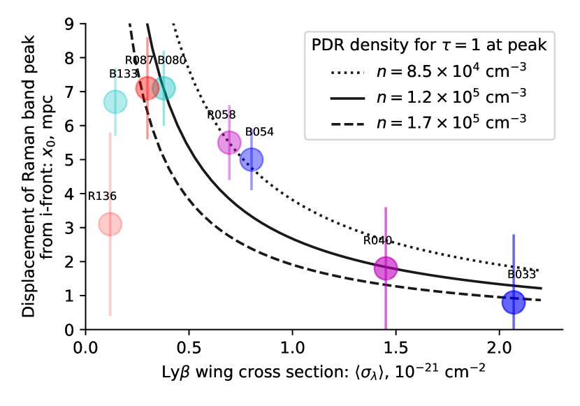
Figure 13: Displacement from the ionization front of the emission peak in each Raman band (column 3 of Table 2), plotted as a function of the cross-section of the $\text{Ly}\beta$ wing (column 6 of Table 1). Color scheme is as in Fig. 3 with error bars showing 10% of the peak FWHM (column 4 of Table 2). Black lines show a simple model in which the peaks occur at $\tau=1$ for 3 different constant neutral hydrogen densities, as indicated in the legend.

4.2.2 Optically thick limit

An independent way of discriminating between optically thick and thin scattering is to look at the spatial distribution of the Raman-scattered intensity. In the optically thin limit, this will simply track the spatial distribution of scatterers and so should not vary between the Raman bands. In the optically thick limit, on the other hand, the scattered light will typically arise at $\tau_{1}\approx 1$, as I will now demonstrate.

Consider a simplified plane-parallel geometry, as depicted in Figure 11. The FUV photons (blue wavy lines) propagate horizontally, with $\tau_{1}$ increasing towards the right. The visual photons propagate vertically (red wavy lines), but I assume here that either $\tau_{2}$ is small or it is independent of $\lambda_{2}$, in which case it will have no differential effect between the Raman bands. If the total FUV optical depth is very large, then from equation (3) the mean value of $\tau_{1}$ weighted by the FUV mean intensity is

$$|\tau_{1}|=\frac{\int_{0}^{\infty}\tau_{1}\,e^{-\tau_{1}}\,d\tau_{1}}{\int_{0}^{\infty}e^{-\tau_{1}}\,d\tau_{1}}=1,$$ (11)

where it is also assumed that $R$ does not vary significantly with $\tau_{1}$. If, in addition, $n(\mathrm{H^{0}})$ and the line-of-sight path length are roughly constant, then from equations (6, 7) the mean $\tau_{1}$ weighted by the observed intensity $I_{\lambda}(\lambda_{2})$ is also $|\tau_{1}|\approx 1$.

4.2.3 Raman scattering as a diagnostic of the neutral hydrogen density in the PDR

Based on the results of the previous section, one would expect that the peak Raman emission should occur for a $\text{Ly}\beta$ wing optical depth of $\tau_{1}\approx 1$ for each band if the scattering is optically thick. Disregarding dust opacity for the time being, this corresponds to a displacement from the ionization front that varies as $x_{0}\approx(n(\mathrm{H^{0}})\langle\sigma_{\lambda}\rangle)^{-1}$, where $n(\mathrm{H^{0}})$ is the neutral hydrogen density in the PDR and $\langle\sigma_{\lambda}\rangle$ is the $\text{Ly}\beta$ wing cross section for the FUV wavelengths that pump each band, which is given in column 6 of Table 1. In Figure 13, this relationship is compared with the measurements of the Orion Bar given in section 2.5. under the assumption that $n(\mathrm{H^{0}})$ is constant over the depth range $2\text{\,}\mathrm{m}\mathrm{p}\mathrm{c}8\text{\,}\mathrm{m}\mathrm{p}\mathrm{c}$. It can be seen that a PDR density of order $n(\mathrm{H^{0}})\sim$1\text{\times}{10}^{5}\text{\,}\mathrm{c}\mathrm{m}^{-3}$$ provides a good fit to the observations for bands within about $\pm 80\text{\,}\mathrm{\SIUnitSymbolAngstrom}$ of line center. A systematic uncertainty of 10% of the width of each emission peak is assigned to the $x_{0}$ values, which has the largest relative impact on the near-wing bands: B033 and R040. As a result, it is the B054 and R058 bands that are the most reliable indicators, yielding $n(\mathrm{H^{0}})=$8.5\text{\times}{10}^{4}\text{\,}\mathrm{c}\mathrm{m}^{-3}$$ (dotted line). This density is similar to that derived from the ratio of intensities of far-infrared [$\mathrm{C\,\scriptstyle II}$] $158\text{\,}\mathrm{\SIUnitSymbolMicro}\mathrm{m}$ and [$\mathrm{O\,\scriptstyle I}$] $145\text{\,}\mathrm{\SIUnitSymbolMicro}\mathrm{m}$ emission lines (Bernard-Salas et al., 2012), which trace slightly deeper layers of the PDR (see Figure 5 and Table 2). Densities derived from molecular hydrogen emission lines show a great deal of variation: Luhman et al. (1998) find densities of ${10}^{5}\text{\,}\mathrm{c}\mathrm{m}^{-3}$ to ${10}^{6}\text{\,}\mathrm{c}\mathrm{m}^{-3}$, whereas Kaplan et al. (2017) favor densities lower than ${10}^{4}\text{\,}\mathrm{c}\mathrm{m}^{-3}$. It has been proposed that the Orion Bar PDR is highly inhomogeneous and clumpy (Burton et al., 1990), but there is little evidence of clumpiness in the distribution of Raman-scattered emission (Figure 4), nor in the mid-infrared PAH and dust emission (Salgado et al., 2012). This suggests that the shallow regions of the PDR, with column densities up to ${10}^{21}\text{\,}\mathrm{c}\mathrm{m}^{-2}$, are relatively smooth.

The displacements of bands in the farther wings fall below the predicted curve, significantly so for B133 and R136. This is an indication that the farther bands may be optically thin instead of optically thick, with the transition occurring near the wavelength of the B080 and R087 bands. It is interesting that this is the same conclusion that is suggested from analysis of the red wing of the compensated spectrum shown in Figure 12, see section 4.2.1 above. If this is the case, then it implies that the total $\mathrm{H^{0}}$ column density through the Orion Bar PDR is $\approx$2\text{\times}{10}^{21}\text{\,}\mathrm{c}\mathrm{m}^{-2}$$. However, an alternative interpretation could be that in these farther bands the $\text{Ly}\beta$ wing cross-section falls below the dust extinction cross-section, so that most FUV photons are absorbed by dust before they can be Raman scattered. In this scenario, the implication would be that $\sigma_{\text{dust}}\approx$5\text{\times}{10}^{-22}\text{\,}\mathrm{c}\mathrm{m}^{2}\,\mathrm{H}^{-1}$$. It is difficult to discriminate between these two possibilities, especially since the dust opacity probably plays a role in determining the size of the $\mathrm{H^{0}}$ column via the position of the molecular hydrogen dissociation front (Draine & Bertoldi, 1996). The FUV dust absorption cross section implied by the Raman scattering is within the range predicted for dense clouds (Cardelli et al., 1989), although Salgado et al. (2016) find that a lower value of $\sigma_{\text{dust}}\approx$1.6\text{\times}{10}^{-22}\text{\,}\mathrm{c}\mathrm{m}^{2}\,\mathrm{H}^{-1}$$ better reproduces the distribution of PAH emission in the Orion Bar. More detailed radiative transfer modeling is required to resolve the issue.

4.3 Absorption features in the Raman pseudo-continuum

The absorption lines seen in the Raman-scattered wings are at STP visual-band wavelengths of $\lambda_{2}=6633$ and $6664\text{\,}\mathrm{\SIUnitSymbolAngstrom}$, which correspond to vacuum FUV wavelengths of $\lambda_{1}=1027$ and $1028\text{\,}\mathrm{\SIUnitSymbolAngstrom}$. In Appendix A it is shown that these can be identified as resonant transitions from the ground state of atomic oxygen: $\mathrm{O\,\scriptstyle I}\ \mathrm{2s2p^{4}\ {}^{3}P}\to\mathrm{2s2p^{3}3d\ ^{3}D^{o}}$. The implication is that the line absorption occurs before the photon is Raman-scattered, and therefore contributes to $\tau_{1}$ (see section 4.1).

The physical location of this $\mathrm{O\,\scriptstyle I}$ absorption is very well constrained observationally because these very same resonance lines (part of the UV 4 multiplet; Moore, 1976) are responsible for pumping some of the strongest visual/IR fluorescent emission lines seen in the nebula. Once excited to $\mathrm{3d\ ^{3}D^{o}}$, the oxygen atom will decay back to the ground level with branching ratio 72.5% via re-emission of an FUV photon, or to the $\mathrm{3p\ ^{3}P}$ level with branching ratio 27.5% via emission of a near-infrared $1.129\text{\,}\mathrm{\SIUnitSymbolMicro}\mathrm{m}$ photon (see Fig. 9 of Walmsley et al., 2000). From $\mathrm{3p\ ^{3}P}$, the only option is decay to $\mathrm{3s\ ^{3}S^{o}}$ via emission of $8446\text{\,}\mathrm{\SIUnitSymbolAngstrom}$ and then back to ground via emission of $1304\text{\,}\mathrm{\SIUnitSymbolAngstrom}$. The spatial distribution of the $8446\text{\,}\mathrm{\SIUnitSymbolAngstrom}$ emission line (see Figures 4c and 5c) should therefore trace the location of the FUV $\mathrm{O\,\scriptstyle I}$ absorption.

It was shown in the section 2, that this fluorescent emission arises very close to the ionization front in all cases and tends to be arranged into filamentary structures that criss-cross the nebula (red channel in Figure 4c), of which the Orion Bar is the most prominent example. As discussed in section 2.5.1, the pumping should be most efficient at a hydrogen column density of $\approx${10}^{19}\text{\,}\mathrm{c}\mathrm{m}^{-2}$$, which is much smaller than the columns of $>$5\text{\times}{10}^{20}\text{\,}\mathrm{c}\mathrm{m}^{-2}$$ where the Raman scattering occurs.

Note that it has long been recognised (Grandi, 1975; Bautista, 1999) that it is the stellar continuum radiation that excites the fluorescent $\mathrm{O\,\scriptstyle I}$ lines in the Orion Nebula. To the contrary, Dopita et al. (2016) propose that the excitation is due to the $\text{Ly}\beta$ $1025.72\text{\,}\mathrm{\SIUnitSymbolAngstrom}$ emission line via the coincidence in wavelength with the $1025.76\text{\,}\mathrm{\SIUnitSymbolAngstrom}$ $\mathrm{O\,\scriptstyle I}$ line. However, although this “photoexcitation by accidental resonance” (PAR) process (Kastner & Bhatia, 1995) is well attested in novae and Herbig Ae/Be stars (Mathew et al., 2018), it requires the $\text{H}\alpha$ transition to be optically thick, which is never the case for $\mathrm{H\,\scriptstyle II}$ regions. Powerful empirical arguments against the PAR process operating in the nebula are (1) that $1.316\text{\,}\mathrm{\SIUnitSymbolMicro}\mathrm{m}$ is stronger than $1.129\text{\,}\mathrm{\SIUnitSymbolMicro}\mathrm{m}$ (Walmsley et al., 2000) and (2) the presence of lines originating from $\mathrm{O\,\scriptstyle I}$ levels as high as $\mathrm{11s}$, such as $4980\text{\,}\mathrm{\SIUnitSymbolAngstrom}$ (Esteban et al., 2004).

4.3.1 Absorption equivalent widths in the FUV frame

The visual-band absorption equivalent width $W_{\lambda}^{\text{obs}}(6633)$ is tightly correlated with the relative brightness $R_{\text{wing}}$ of the Raman wings (section 2.6.1). Taking the ratio of these, one obtains $W_{\lambda}^{\text{Raman}}(6633)=W_{\lambda}^{\text{obs}}(6633)/R_{\text{wing}}$, which is an equivalent width normalized to only the Raman pseudo-continuum itself, rather than the full nebular continuum. This is roughly constant across the nebula at $W_{\lambda}^{\text{Raman}}(6633)=$2.2\pm 1.0\text{\,}\mathrm{\SIUnitSymbolAngstrom}$$ (see Figure 7). The equivalent width of the FUV absorption line is then smaller than $W_{\lambda}^{\text{Raman}}(6633)$ by a factor of $(\lambda_{2}/\lambda_{1})^{2}\approx 41$, yielding $W_{\lambda}^{\text{FUV}}(1027)\approx$0.05\text{\,}\mathrm{\SIUnitSymbolAngstrom}$$. If the line profile is Gaussian, then the relation between velocity FWHM, $\Delta V$, and equivalent width is $W_{\lambda}=1.064A_{0}\lambda_{0}\Delta V/c$, where $A_{0}$ is the relative absorption depth at line center. Assuming complete absorption ($A_{0}=1$), then yields $\Delta V=$15\pm 6\text{\,}\mathrm{k}\mathrm{m}\,\mathrm{s}^{-1}$$. Very similar velocity widths were found for the $6664\text{\,}\mathrm{\SIUnitSymbolAngstrom}$ absorption feature from the high-resolution Keck spectra (Table 3).

4.3.2 The failure of rival explanations for the 6633, 6664 Å lines

However strong the case for identifying the absorption features at $6633$ and $6664\text{\,}\mathrm{\SIUnitSymbolAngstrom}$ with Raman-scattered FUV $\mathrm{O\,\scriptstyle I}$ absorption lines, it is nonetheless important to thoroughly investigate potential competing explanations, if only to rule them out.

Why they cannot be dust-scattered stellar absorption lines

Various photospheric absorption lines of luminous O stars are visible in the spectrum of the diffuse nebula due to scattering of the starlight by dust grains in the $\mathrm{H\,\scriptstyle II}$ region and surrounding PDR. These are clearest in the case of high-ionization lines that are absent from the emission spectrum of the nebular gas, such as the $\mathrm{He\,\scriptstyle II}$ and $\mathrm{C\,\scriptstyle IV}$ lines that were analysed above in § 2.6.2. At first glance, it might seem that the equivalent width map of the $6633\text{\,}\mathrm{\SIUnitSymbolAngstrom}$ feature (Figure 6a) is similar to that of the $\mathrm{C\,\scriptstyle IV}$ absorption lines (Figure 6e). However, there are important differences: the ridge of peak $\mathrm{C\,\scriptstyle IV}$ absorption lies at about $20$ to $30\text{\,}\mathrm{a}\mathrm{r}\mathrm{c}\mathrm{s}\mathrm{e}\mathrm{c}$ from the Trapezium stars, close to the “Trap SW” region shown in Figure 2b, whereas the $6633\text{\,}\mathrm{\SIUnitSymbolAngstrom}$ absorption ridges lie farther from the Trapezium ($50$ to $60\text{\,}\mathrm{a}\mathrm{r}\mathrm{c}\mathrm{s}\mathrm{e}\mathrm{c}$) in the “SW minibar” and “Orion S” regions. This implies that the spatial distribution of scatterers is different between the two cases. This is exactly what would be expected under the Raman-scattering hypothesis for $6633\text{\,}\mathrm{\SIUnitSymbolAngstrom}$, since the scatterers are neutral hydrogen atoms, located in the PDR outside the $\mathrm{H\,\scriptstyle II}$ region, whereas the stellar continuum is scattered by dust grains, some of which will be inside the $\mathrm{H\,\scriptstyle II}$ region.

An even stronger argument against a visual-band stellar origin is that no absorption features at $6633$ or $6664\text{\,}\mathrm{\SIUnitSymbolAngstrom}$ are seen in the luminous OB stars of the nebula. The closest match is a pair of $\mathrm{Fe\,\scriptstyle I}$ features at $6634$ and $6664\text{\,}\mathrm{\SIUnitSymbolAngstrom}$, which are seen in absorption in the photospheres of several K and M-type T Tauri stars in the Orion Nebula cluster. One of the brightest and most centrally located examples is V2279 Ori (Parenago 1869, JW 499, TCC 52), a visual binary (spectral type M0.5 + M2; Daemgen et al., 2012) which is the central star of the prominent proplyd 159-350 (HST 3; O’Dell et al., 1993). However, the luminosity of this source is only $\approx$10\text{\,}\mathrm{\text{L${}_{\odot}$}}$$ and its brightness around $6650\text{\,}\mathrm{\SIUnitSymbolAngstrom}$ is 200 times smaller than that of $\theta^{1}\,\text{Ori\leavevmode\nobreak\ C}$. Furthermore, photospheric lines are weak in T Tauri stars due to accretion veiling and the equivalent widths of these absorption features are only $W_{\lambda}^{\star}\approx$0.1\text{\,}\mathrm{\SIUnitSymbolAngstrom}$$. Therefore, even several such stars would contribute at most $0.001\text{\,}\mathrm{\SIUnitSymbolAngstrom}$ to the equivalent width in the diffuse nebular spectrum, which is far less than the observed values $W_{\lambda}^{\text{obs}}=$0.1\text{\,}\mathrm{\SIUnitSymbolAngstrom}$$ to $0.5\text{\,}\mathrm{\SIUnitSymbolAngstrom}$ (Figure 7).

Why they are unlikely to be visual-band neutral/molecular absorption lines from the PDR

The fact that the $6633$ and $6664\text{\,}\mathrm{\SIUnitSymbolAngstrom}$ features are not seen in the spectra of the luminous stars, such as $\theta^{1}\,\text{Ori\leavevmode\nobreak\ C}$, means that they cannot arise in the foreground neutral gas of the Orion veil (Abel et al., 2004; Abel et al., 2019). However, if some neutral or molecular species were abundant in the dense PDR behind the nebula, but not in the Veil, then it is theoretically possible that it might imprint an absorption signature on the starlight that initially enters the PDR but is then reflected out again by dust scattering. On the other hand, such a scenario seems very far-fetched and I have been unable to find any candidate absorption features at relevant wavelengths.

Why they cannot be solid-state absorption features

The same argument as in the previous paragraph also rules out any possibility that foreground DIB absorption might be responsible for these features, with the additional argument that the $6633\text{\,}\mathrm{\SIUnitSymbolAngstrom}$ equivalent width does not correlate with foreground extinction, as the known DIB at $5780\text{\,}\mathrm{\SIUnitSymbolAngstrom}$ does. However, that leaves open the possibility of the contrived back-scattering scenario discussed above. There is a DIB at $6632.85\text{\,}\mathrm{\SIUnitSymbolAngstrom}$ (Galazutdinov et al., 2000), which is consistent in wavelength with the $6633\text{\,}\mathrm{\SIUnitSymbolAngstrom}$ feature but it is only seen in highly-reddened stars and is always at least 10 times weaker than the $5780\text{\,}\mathrm{\SIUnitSymbolAngstrom}$ feature. From Figure 8 it is conceivable that up to half of the $5780\text{\,}\mathrm{\SIUnitSymbolAngstrom}$ absorption might arise during back-scattering from the PDR rather than in foreground material for some sight lines. This would imply an equivalent width $W_{\lambda}<$0.02\text{\,}\mathrm{\SIUnitSymbolAngstrom}$$ for the $6632.85\text{\,}\mathrm{\SIUnitSymbolAngstrom}$ DIB, which is again much smaller than the observed $W_{\lambda}^{\text{obs}}(6633)=0.1$ to $0.5\text{\,}\mathrm{\SIUnitSymbolAngstrom}$ (Figure 7).

4.3.3 Possible detection of a $6481\text{\,}\mathrm{\SIUnitSymbolAngstrom}$ absorption feature

A further absorption line is tentatively detected at $6481\text{\,}\mathrm{\SIUnitSymbolAngstrom}$ in the B080 Raman band (see Figure 3), which could correspond to one of the components of the $\mathrm{Si\,\scriptstyle II}$ $\mathrm{3s^{2}3p\ ^{2}P^{o}}\to\mathrm{3s^{2}5s\ ^{2}S}$ doublet (the other component, at $6362\text{\,}\mathrm{\SIUnitSymbolAngstrom}$ is hidden by a much stronger [$\mathrm{O\,\scriptstyle I}$] emission line at $6363\text{\,}\mathrm{\SIUnitSymbolAngstrom}$). This doublet (vacuum FUV wavelengths $1020.7$ and $1023.7\text{\,}\mathrm{\SIUnitSymbolAngstrom}$) pumps the visual-band fluorescent emission lines $5957.6$ and $5978.9\text{\,}\mathrm{\SIUnitSymbolAngstrom}$. The distribution of the $5978.9\text{\,}\mathrm{\SIUnitSymbolAngstrom}$ line is significantly different from the $\mathrm{O\,\scriptstyle I}$ fluorescent lines, being more similar to singly-ionized forbidden lines such as [$\mathrm{S\,\scriptstyle II}$] and [$\mathrm{N\,\scriptstyle II}$]. This is what would be expected since $\mathrm{Si^{+}}$, unlike $\mathrm{O^{0}}$, has a significant column inside the ionized gas.

The $6481\text{\,}\mathrm{\SIUnitSymbolAngstrom}$ feature is considerably weaker than the other absorption features and is located in a more complicated region of the spectrum, which makes it difficult to make quantitative measurements. Note that Dopita et al. (2016) claim evidence of a broad emission bump in the blue Raman wing, centered on the $\mathrm{Si\,\scriptstyle II}$ $6481\text{\,}\mathrm{\SIUnitSymbolAngstrom}$ wavelength. However, I find no clear evidence for such a bump in the Orion MUSE or Keck spectra.

5 Summary

By analysing spatially resolved spectroscopic observations of the Orion Nebula, I have demonstrated that the broad Raman-scattered wings of the $\text{H}\alpha$ $6563\text{\,}\mathrm{\SIUnitSymbolAngstrom}$ line ($\delta\lambda=$\pm 150\text{\,}\mathrm{\SIUnitSymbolAngstrom}$$) are a useful diagnostic of the interaction of far-ultraviolet radiation with atomic hydrogen in the environs of high-mass stars. The principal conclusions of this study are:

1. Hydrogen Raman scattering of starlight from $\text{Ly}\beta$ to $\text{H}\alpha$ wings occurs in the neutral photo-dissociation region (PDR), located between the hydrogen ionization front and dissociation front.

2. The inner Raman wings ($|\delta\lambda|<$80\text{\,}\mathrm{\SIUnitSymbolAngstrom}$$) of $\text{H}\alpha$ are optically thick and allow the density of neutral hydrogen atoms to be determined in edge-on PDRs. For the case of the Orion Bar, I find $n(\mathrm{H^{0}})\approx${10}^{5}\text{\,}\mathrm{c}\mathrm{m}^{-3}$$ for the shallow part of the PDR (depths of up to $10\text{\,}\mathrm{m}\mathrm{p}\mathrm{c}$).

3. The outer Raman wings are either optically thin or are limited by competition with dust absorption. In the first case, the total column density of neutral hydrogen must be $2\text{\times}{10}^{21}\text{\,}\mathrm{c}\mathrm{m}^{-2}$ in the Orion Bar. In the second case, the FUV dust absorption cross section must be $5\text{\times}{10}^{-22}\text{\,}\mathrm{c}\mathrm{m}^{2}\,\mathrm{H}^{-1}$.

4. Far-ultraviolet resonance lines of neutral oxygen imprint their absorption onto the stellar continuum as it passes through the ionization front. The subsequent Raman scattering of this continuum yields absorption lines in the red $\text{H}\alpha$ wing at transformed wavelengths of $6633\text{\,}\mathrm{\SIUnitSymbolAngstrom}$ and $6664\text{\,}\mathrm{\SIUnitSymbolAngstrom}$. This is a unique signature of Raman scattering, which allows it to be easily distinguished from other processes that might produce broad $\text{H}\alpha$ wings, such as electron scattering or high-velocity outflows.

5. The widths of the Raman-scattered absorption lines are of order $2\text{\,}\mathrm{\SIUnitSymbolAngstrom}$, which would correspond to a velocity width of $100\text{\,}\mathrm{k}\mathrm{m}\,\mathrm{s}^{-1}$ in the visual band, but only $15\text{\,}\mathrm{k}\mathrm{m}\,\mathrm{s}^{-1}$ in the FUV band where the lines were formed. This “magnification” of Doppler velocity scales by the Raman scattering process allows spectrographs to operate at a $6.4$ times higher effective spectral resolution, but observations with better signal-to-noise than are currently available are required in order to take full advantage of this.

Data availability

The primary data underlying this article are two spectroscopic datasets. First, integral field spectral mosaics of the inner Orion Nebula, obtained with the MUSE spectrograph on the VLT, which are available from http://muse-vlt.eu/science/m42/. Second, longslit spectra of the Orion S region, obtained with the HIRES spectrograph on the Keck I telescope, which are available from the Keck Observatory Archive at https://koa.ipac.caltech.edu/cgi-bin/KOA/nph-KOAlogin. Additional supporting data from other observatories and archives may be accessed via the references given in the main text. All data reduction and analysis programs used in this paper, together with documentation and research notes may be found at https://github.com/will-henney/dib-scatter-hii.

Appendix A Raman scattering theory

Table 4: FUV/optical wavelength equivalencies for Raman scattering

Ion	Transition	$J_{i}\to J_{k}$	$\lambda_{1},\ $\mathrm{\SIUnitSymbolAngstrom}$$	$\tilde{\nu}_{1},\ $\mathrm{c}\mathrm{m}^{-1}$$	$\Delta\tilde{\nu},\ $\mathrm{c}\mathrm{m}^{-1}$$	$\tilde{\nu}_{2},\ $\mathrm{c}\mathrm{m}^{-1}$$	$\lambda_{2},\ $\mathrm{\SIUnitSymbolAngstrom}$$	$\lambda_{\text{air}},\ $\mathrm{\SIUnitSymbolAngstrom}$$
			$\quad\text{Ly}\beta,\ n=1\quad$			$\quad\text{H}\alpha,\ n=2\quad$
$\mathrm{H\,\scriptstyle I}$	$n\mathrm{s\ ^{2}S}\to\mathrm{3p\ ^{2}P}$	$1/2\to 1/2,3/2$	$1025.72220$	$97492.283$	$0.000$	$15233.329$	$6564.553$	$6562.740$
$\mathrm{O\,\scriptstyle I}$	$\mathrm{2s^{2}2p^{4}\ {}^{3}P}\to\mathrm{2s^{2}2p^{3}(^{4}S)3d\ ^{3}D^{o}}$	$0\to 1$	$1028.15729$	$97261.383$	$-230.900$	$15002.429$	$6665.587$	$6663.747$
		$1\to 1$	$1027.43139$	$97330.100$	$-162.183$	$15071.146$	$6635.196$	$6633.364$
		$1\to 2$	$1027.43077$	$97330.159$	$-162.124$	$15071.205$	$6635.170$	$6633.338$
		$2\to 1$	$1025.76339$	$97488.369$	$-3.914$	$15229.415$	$6566.240$	$6564.427$
		$2\to 2$	$1025.76276$	$97488.429$	$-3.854$	$15229.475$	$6566.215$	$6564.401$
		$2\to 3$	$1025.76170$	$97488.530$	$-3.753$	$15229.576$	$6566.171$	$6564.358$
$\mathrm{Si\,\scriptstyle II}$	$\mathrm{3s^{2}3p\ ^{2}P^{o}}\to\mathrm{3s^{2}5s\ ^{2}S}$	$1/2\to 1/2$	$1020.6989$	$97972.086$	$+479.803$	$15713.132$	$6364.104$	$6362.345$
		$1/2\to 3/2$	$1023.7001$	$97684.859$	$192.576$	$15425.905$	$6482.602$	$6480.811$

When a photon is Raman-scattered from the vicinity of $\text{Ly}\beta$ (UV domain) to the vicinity of $\text{H}\alpha$ (optical domain) its wavelength is transformed from $\lambda_{1}$ to $\lambda_{2}$. Intervals in frequency ($\nu=c/\lambda$) or wavenumber ($\tilde{\nu}=1/\lambda$) space are conserved between the two domains. For example the wavenumber displacement from the $\mathrm{H\,\scriptstyle I}$ line center can be written in two ways:

$$\Delta\tilde{\nu}=\tilde{\nu}_{1}-\tilde{\nu}(\text{Ly}\beta)=\tilde{\nu}_{2}-\tilde{\nu}(\text{H}\alpha)\ ,$$ (12)

from which it follows that

$$\lambda_{2}=\left(\frac{1}{\lambda(\text{H}\alpha)}+\frac{1}{\lambda_{1}}-\frac{1}{\lambda(\text{Ly}\beta)}\right)^{-1}\ .$$ (13)

The wavelengths $\lambda(\text{Ly}\beta)$ and $\lambda(\text{H}\alpha)$, together with their corresponding wavenumbers, are given in Table 4 (all wavelengths are on the vacuum scale unless otherwise noted). For both lines, a weighted average over the $\mathrm{3p\ ^{2}P_{1/2}}$ and $\mathrm{3p\ ^{2}P_{3/2}}$ upper levels is used, assumed to be populated according to their statistical weights, with individual component wavelengths obtained from Tab. XXVIII of Mohr et al. (2008). Note that the electric dipole selection rules mean that only $\mathrm{3p\to 2s}$ transitions contribute to $\text{H}\alpha$ in the Raman scattering context. The wavelength is therefore slightly shorter than the value obtained for the $\text{H}\alpha$ recombination line, which includes additional contributions from $\mathrm{3s\to 2p}$ and $\mathrm{3d\to 2p}$. The shift is of order $-0.05\text{\,}\mathrm{\SIUnitSymbolAngstrom}$ or $-2\text{\,}\mathrm{k}\mathrm{m}\,\mathrm{s}^{-1}$ with respect to the Case B results reported in Tab. 6a of Clegg et al. (1999).

Also listed in Table 4 are the Raman transformations $\lambda_{1}\to\lambda_{2}$ for the rest wavelengths of transitions between the ground $\mathrm{2s^{2}2p^{4}\ {}^{3}P}$ term of neutral $\mathrm{{}^{16}O}$ and the excited $\mathrm{2s^{2}2p^{3}3d\ ^{3}D^{o}}$ term. The $\mathrm{O\,\scriptstyle I}$ data is obtained from highly accurate laser metrology (Ivanov et al., 2008; Marinov et al., 2017), with a precision of $0.08\text{\,}\mathrm{c}\mathrm{m}^{-1}$ or better. The fine structure splitting between the $J_{k}$ levels of the excited term ($\sim$0.1\text{\,}\mathrm{c}\mathrm{m}^{-1}$$) is much smaller than that between the $J_{i}$ levels of the ground term ($\sim$100\text{\,}\mathrm{c}\mathrm{m}^{-2}$$), so that the 6 transitions fall into 3 well-separated groups. The three transitions from the lowest energy $J_{i}=2$ level are very close to $\text{Ly}\beta$ ($\Delta\tilde{\nu}\approx$4\text{\,}\mathrm{c}\mathrm{m}^{-1}$$), whereas the two transitions from $J_{i}=1$ ($\Delta\tilde{\nu}\approx$162\text{\,}\mathrm{c}\mathrm{m}^{-1}$$) and the single transition from $J_{i}=0$ ($\Delta\tilde{\nu}\approx$231\text{\,}\mathrm{c}\mathrm{m}^{-1}$$) lie increasingly to the red. The corresponding wavelengths in the optical domain, $\lambda_{2}$, are therefore on the red side of $\text{H}\alpha$. The final column of the table uses STP refractive indices (Greisen et al., 2006) to convert $\lambda_{2}$ to air wavelengths, $\lambda_{\text{air}}$, for ease of comparison with ground-based optical spectroscopy. The resultant wavelength is $6663.747\text{\,}\mathrm{\SIUnitSymbolAngstrom}$ for the line from $J_{i}=0$, with an uncertainty of about $0.004\text{\,}\mathrm{\SIUnitSymbolAngstrom}$, which is much smaller than typical observational precision (for instance, $0.07\text{\,}\mathrm{\SIUnitSymbolAngstrom}$ for a very high resolution spectrograph with resolving power of $R=${10}^{5}$$). The two lines from $J_{i}=1$, with a separation of $0.028\text{\,}\mathrm{\SIUnitSymbolAngstrom}$, will always be blended in observations, giving a mean wavelength of $6633.347\text{\,}\mathrm{\SIUnitSymbolAngstrom}$ (assuming the upper levels are distributed according to statistical weight $2J_{k}+1$). Similarly, the three lines from $J_{i}=2$ have a mean wavelength of $6564.386\text{\,}\mathrm{\SIUnitSymbolAngstrom}$, but this is so close to $\text{H}\alpha$ (corresponding to a Doppler shift of $+75\text{\,}\mathrm{k}\mathrm{m}\,\mathrm{s}^{-1}$) that it would be very difficult to observe.

The final section of Table 4 gives data for a resonance doublet of $\mathrm{Si^{+}}$ whose components lie a few $\mathrm{\SIUnitSymbolAngstrom}$ to the blue of $\text{Ly}\beta$. The shorter of the two components is Raman-transformed to $\lambda_{\text{air}}=$6362.35\text{\,}\mathrm{\SIUnitSymbolAngstrom}$$, which unfortunately coincides with the collisionally excited [$\mathrm{O\,\scriptstyle I}$] line at $6363.78\text{\,}\mathrm{\SIUnitSymbolAngstrom}$. The longer component is transformed to $6480.81\text{\,}\mathrm{\SIUnitSymbolAngstrom}$ in a region that is clear of any strong nebular lines. Wavelengths for these lines are based on energy levels from Martin & Zalubas (1983), with an estimated precision of $0.1\text{\,}\mathrm{c}\mathrm{m}^{-1}$, which gives an uncertainty in the optical wavelengths $\lambda_{2}$ of $0.04\text{\,}\mathrm{\SIUnitSymbolAngstrom}$.

The total cross-section for the off-resonance $\mathrm{1s\to 3p}$ transition in $\mathrm{H^{0}}$ is calculated in § 2 of Chang et al. (2015) from second order time-dependent perturbation theory. Results are presented in the upper panel of Figure 1 of that paper in terms of a Doppler velocity factor $\Delta V_{1}$, which in the notation of the current paper is

$$\Delta V_{1}=c\left(\frac{\lambda_{1}}{\lambda(\text{Ly}\beta)}-1\right)\ .$$ (14)

The observed Raman-scattered wings of $\text{H}\alpha$ that are analyzed in this paper are typically within $\Delta\lambda_{2}\sim\pm$100\text{\,}\mathrm{\SIUnitSymbolAngstrom}$$ of the line core. It is therefore convenient to define a dimensionless wavelength in the optical domain as

$$x=\frac{\lambda_{2}-\lambda(\text{H}\alpha)}{$100\text{\,}\mathrm{\SIUnitSymbolAngstrom}$}\ ,$$ (15)

which corresponds to $x\approx\Delta V_{1}/$714\text{\,}\mathrm{k}\mathrm{m}\,\mathrm{s}^{-1}$$ in the FUV domain. The total cross section in the range $0.4<|x|<2.3$ can then be fit as follows:

$$\frac{\sigma}{${10}^{-21}\text{\,}\mathrm{c}\mathrm{m}^{2}$}=\begin{cases}0.2186x^{-2}-0.0344x^{-1}-0.0054&\text{if $x<0$}\\ 0.2367x^{-2}-0.0187x^{-1}+0.0004&\text{if $x>0$}\end{cases}$$ (16)

Note that separate fits are given for the blue ($x<0$) and red ($x>0$) wings of $\text{H}\alpha$ since the cross section, although approximately Lorentzian, is not exactly symmetric, being stronger on the blue side (by about 10% for $x=\pm 1$).

The fraction of all $\mathrm{1s\to 3p}$ excitations that result in Raman scattering to an optical photon is given by the branching ratio, $f_{\text{H}\alpha}$, with the remaining fraction, $1-f_{\text{H}\alpha}$, resulting in elastic Rayleigh scattering in which the photon remains in the FUV domain. The results for $f_{\text{H}\alpha}$ are also shown in Figure 1 of Chang et al. (2015) and can be fit as follows in the range $|x|<5$:

$$f_{\text{H}\alpha}=0.2238+0.0363x+0.0024x^{2}\ .$$ (17)

The relative accuracy of all these fits is better than 1% within the stated range (corresponding to $\sigma\approx\text{${10}^{-22}\text{\,}\mathrm{c}\mathrm{m}^{2}{10}^{-21}\text{\,}\mathrm{c}\mathrm{m}^{2}$}$), which is perfectly adequate for the purposes of this paper. Note that the branching ratio increases with $x$, which means that the product $\sigma f_{\text{H}\alpha}$ is stronger on the red side of $\text{H}\alpha$.

References

- Abel et al. (2004) Abel N. P., Brogan C. L., Ferland G. J., O’Dell C. R., Shaw G., Troland T. H., 2004, ApJ, 609, 247
- Abel et al. (2019) Abel N. P., Ferland G. J., O’Dell C. R., 2019, ApJ, 881, 130
- Arab et al. (2012) Arab H., Abergel A., Habart E., Bernard-Salas J., Ayasso H., Dassas K., Martin P. G., White G. J., 2012, A&A, 541, A19
- Bacon et al. (2010) Bacon R., et al., 2010, in Proc. SPIE. p. 773508, doi:10.1117/12.856027
- Bacon et al. (2014) Bacon R., et al., 2014, The Messenger, 157, 13
- Baldwin et al. (2000) Baldwin J. A., Verner E. M., Verner D. A., Ferland G. J., Martin P. G., Korista K. T., Rubin R. H., 2000, ApJS, 129, 229
- Bally et al. (2000) Bally J., O’Dell C. R., McCaughrean M. J., 2000, AJ, 119, 2919
- Baron et al. (2015) Baron D., Poznanski D., Watson D., Yao Y., Prochaska J. X., 2015, MNRAS, 447, 545
- Bautista (1999) Bautista M. A., 1999, ApJ, 527, 474
- Bernard-Salas et al. (2012) Bernard-Salas J., et al., 2012, A&A, 538, A37
- Blagrave et al. (2007) Blagrave K. P. M., Martin P. G., Rubin R. H., Dufour R. J., Baldwin J. A., Hester J. J., Walter D. K., 2007, ApJ, 655, 299
- Bregman et al. (1989) Bregman J. D., Allamandola L. J., Tielens A. G. G. M., Geballe T. R., Witteborn F. C., 1989, ApJ, 344, 791
- Burton et al. (1990) Burton M. G., Hollenbach D. J., Tielens A. G. G. M., 1990, ApJ, 365, 620
- Cardelli et al. (1989) Cardelli J. A., Clayton G. C., Mathis J. S., 1989, ApJ, 345, 245
- Cesarsky et al. (2000) Cesarsky D., Jones A. P., Lequeux J., Verstraete L., 2000, A&A, 358, 708
- Chang et al. (2015) Chang S.-J., Heo J.-E., Di Mille F., Angeloni R., Palma T., Lee H.-W., 2015, ApJ, 814, 98
- Clegg et al. (1999) Clegg R. E. S., Miller S., Storey P. J., Kisielius R., 1999, A&AS, 135, 359
- Conti (1972) Conti P. S., 1972, ApJ, 174, L79
- Cordiner et al. (2019) Cordiner M. A., et al., 2019, ApJ, 875, L28
- Da Rio et al. (2009) Da Rio N., Robberto M., Soderblom D. R., Panagia N., Hillenbrand L. A., Palla F., Stassun K., 2009, ApJS, 183, 261
- Daemgen et al. (2012) Daemgen S., Correia S., Petr-Gotzens M. G., 2012, A&A, 540, A46
- Desert et al. (1990) Desert F.-X., Boulanger F., Puget J. L., 1990, A&A, 237, 215
- Donati et al. (2002) Donati J.-F., Babel J., Harries T. J., Howarth I. D., Petit P., Semel M., 2002, MNRAS, 333, 55
- Dopita et al. (2016) Dopita M. A., Nicholls D. C., Sutherland R. S., Kewley L. J., Groves B. A., 2016, ApJ, 824, L13
- Draine & Bertoldi (1996) Draine B. T., Bertoldi F., 1996, ApJ, 468, 269
- Escalante et al. (1991) Escalante V., Sternberg A., Dalgarno A., 1991, ApJ, 375, 630
- Esteban et al. (2004) Esteban C., Peimbert M., García-Rojas J., Ruiz M. T., Peimbert A., Rodríguez M., 2004, MNRAS, 355, 229
- Ferland et al. (2012) Ferland G. J., Henney W. J., O’Dell C. R., Porter R. L., van Hoof P. A. M., Williams R. J. R., 2012, ApJ, 757, 79
- Ferland et al. (2017) Ferland G. J., et al., 2017, Rev. Mex. Astron. Astrofis., 53, 385
- Friedman et al. (2011) Friedman S. D., et al., 2011, ApJ, 727, 33
- Galazutdinov et al. (2000) Galazutdinov G. A., Musaev F. A., Krełowski J., Walker G. A. H., 2000, PASP, 112, 648
- García-Díaz & Henney (2007) García-Díaz M. T., Henney W. J., 2007, AJ, 133, 952
- García-Díaz et al. (2008) García-Díaz M. T., Henney W. J., López J. A., Doi T., 2008, Rev. Mex. Astron. Astrofis., 44, 181
- García-Díaz et al. (2018) García-Díaz M. T., Steffen W., Henney W. J., López J. A., García-López F., González-Buitrago D., Áviles A., 2018, MNRAS, 479, 3909
- Goicoechea et al. (2017) Goicoechea J. R., et al., 2017, A&A, 601, L9
- Grandi (1975) Grandi S. A., 1975, ApJ, 199, L43+
- Greisen et al. (2006) Greisen E. W., Calabretta M. R., Valdes F. G., Allen S. L., 2006, A&A, 446, 747
- Heger (1922) Heger M. L., 1922, Lick Observatory Bulletin, 10, 141
- Henney (1998) Henney W. J., 1998, ApJ, 503, 760
- Henney & O’Dell (1999) Henney W. J., O’Dell C. R., 1999, AJ, 118, 2350
- Henney et al. (2005) Henney W. J., Arthur S. J., Williams R. J. R., Ferland G. J., 2005, ApJ, 621, 328
- Hobbs et al. (2008) Hobbs L. M., et al., 2008, ApJ, 680, 1256
- Ivanov et al. (2008) Ivanov T. I., Salumbides E. J., Vieitez M. O., Cacciani P. C., de Lange C. A., Ubachs W., 2008, MNRAS, 389, L4
- Joye & Mandel (2003) Joye W. A., Mandel E., 2003, in Payne H. E., Jedrzejewski R. I., Hook R. N., eds, Astronomical Society of the Pacific Conference Series Vol. 295, Astronomical Data Analysis Software and Systems XII. p. 489
- Kaplan et al. (2017) Kaplan K. F., et al., 2017, ApJ, 838, 152
- Kassis et al. (2006) Kassis M., Adams J. D., Campbell M. F., Deutsch L. K., Hora J. L., Jackson J. M., Tollestrup E. V., 2006, ApJ, 637, 823
- Kastner & Bhatia (1995) Kastner S. O., Bhatia A. K., 1995, ApJ, 439, 346
- Kissler-Patig et al. (2008) Kissler-Patig M., et al., 2008, A&A, 491, 941
- Kong et al. (2018) Kong S., et al., 2018, ApJS, 236, 25
- Kos & Zwitter (2013) Kos J., Zwitter T., 2013, ApJ, 774, 72
- Kounkel et al. (2017) Kounkel M., et al., 2017, ApJ, 834, 142
- Krełowski & Westerlund (1988) Krełowski J., Westerlund B. E., 1988, A&A, 190, 339
- Krełowski et al. (2019) Krełowski J., Galazutdinov G., Godunova V., Bondar A., 2019, Acta Astron., 69, 159
- Lai et al. (2020) Lai T. S. Y., Witt A. N., Alvarez C., Cami J., 2020, MNRAS, 492, 5853
- Luhman et al. (1998) Luhman K. L., Engelbracht C. W., Luhman M. L., 1998, ApJ, 499, 799
- Marconi et al. (1998) Marconi A., Testi L., Natta A., Walmsley C. M., 1998, A&A, 330, 696
- Marinov et al. (2017) Marinov D., Booth J. P., Drag C., Blondel C., 2017, Journal of Physics B Atomic Molecular Physics, 50, 065003
- Martin & Zalubas (1983) Martin W. C., Zalubas R., 1983, Journal of Physical and Chemical Reference Data, 12, 323
- Massa et al. (2020) Massa D., Fitzpatrick E. L., Gordon K. D., 2020, ApJ, 891, 67
- Mathew et al. (2018) Mathew B., et al., 2018, ApJ, 857, 30
- Maíz Apellániz et al. (2019) Maíz Apellániz J., et al., 2019, A&A, 626, A20
- Mc Leod et al. (2016) Mc Leod A. F., Weilbacher P. M., Ginsburg A., Dale J. E., Ramsay S., Testi L., 2016, MNRAS, 455, 4057
- Megeath et al. (2012) Megeath S. T., et al., 2012, AJ, 144, 192
- Mesa-Delgado et al. (2009) Mesa-Delgado A., Esteban C., García-Rojas J., Luridiana V., Bautista M., Rodríguez M., López-Martín L., Peimbert M., 2009, MNRAS, 395, 855
- Moehler et al. (2014) Moehler S., et al., 2014, A&A, 568, A9
- Mohr et al. (2008) Mohr P. J., Taylor B. N., Newell D. B., 2008, Rev. Mod. Phys., 80, 633
- Moore (1976) Moore C. E., 1976, Nat. Stand. Ref. Data Ser., NBS 3, Section 7, Selected Tables of Atomic Spectra, Atomic Energy Levels and Multiplet Tables – O I. Nat. Bur. Stand., US
- Moré (1978) Moré J. J., 1978, in Watson G. A., ed., Numerical Analysis. Springer Berlin Heidelberg, Berlin, Heidelberg, pp 105–116
- Noll et al. (2012) Noll S., Kausch W., Barden M., Jones A. M., Szyszka C., Kimeswenger S., Vinther J., 2012, A&A, 543, A92
- Noll et al. (2014) Noll S., Kausch W., Kimeswenger S., Barden M., Jones A. M., Modigliani A., Szyszka C., Taylor J., 2014, A&A, 567, A25
- Nussbaumer et al. (1989) Nussbaumer H., Schmid H. M., Vogel M., 1989, A&A, 211, L27
- O’Dell & Yusef-Zadeh (2000) O’Dell C. R., Yusef-Zadeh F., 2000, AJ, 120, 382
- O’Dell et al. (1993) O’Dell C. R., Wen Z., Hu X., 1993, ApJ, 410, 696
- O’Dell et al. (2017) O’Dell C. R., Ferland G. J., Peimbert M., 2017, MNRAS, 464, 4835
- Omont et al. (2019) Omont A., Bettinger H. F., Tönshoff C., 2019, A&A, 625, A41
- Osterbrock & Ferland (2006) Osterbrock D. E., Ferland G. J., 2006, Astrophysics of gaseous nebulae and active galactic nuclei, second edn. Sausalito, CA: University Science Books
- Osterbrock et al. (1996) Osterbrock D. E., Fulbright J. P., Martel A. R., Keane M. J., Trager S. C., Basri G., 1996, PASP, 108, 277
- Parikka et al. (2018) Parikka A., Habart E., Bernard-Salas J., Köhler M., Abergel A., 2018, A&A, 617, A77
- Salgado et al. (2012) Salgado F., et al., 2012, ApJ, 749, L21
- Salgado et al. (2016) Salgado F., Berné O., Adams J. D., Herter T. L., Keller L. D., Tielens A. G. G. M., 2016, ApJ, 830, 118
- Schmid (1989) Schmid H. M., 1989, A&A, 211, L31
- Shenstone (1970) Shenstone A. G., 1970, Journal of research of the National Bureau of Standards. Section A, Physics and chemistry, 74A, 801
- Simón-Díaz et al. (2006) Simón-Díaz S., Herrero A., Esteban C., Najarro F., 2006, A&A, 448, 351
- Smette et al. (2015) Smette A., et al., 2015, A&A, 576, A77
- Smith et al. (2005) Smith N., Bally J., Shuping R. Y., Morris M., Kassis M., 2005, AJ, 130, 1763
- Sonnentrucker (2014) Sonnentrucker P., 2014, in Cami J., Cox N. L. J., eds, IAU Symposium Vol. 297, The Diffuse Interstellar Bands. pp 13–22, doi:10.1017/S1743921313015524
- Stahl et al. (1993) Stahl O., Wolf B., Gang T., Gummersbach C. A., Kaufer A., Kovacs J., Mandel H., Szeifert T., 1993, A&A, 274, L29
- Stahl et al. (1996) Stahl O., et al., 1996, A&A, 312, 539
- Subrahmanyan et al. (2001) Subrahmanyan R., Goss W. M., Malin D. F., 2001, AJ, 121, 399
- Tielens (2014) Tielens A. G. G. M., 2014, in Cami J., Cox N. L. J., eds, IAU Symposium Vol. 297, The Diffuse Interstellar Bands. pp 399–411, doi:10.1017/S1743921313016207
- Van Hoof (2018) Van Hoof P. A. M., 2018, Galaxies, 6
- Virtanen et al. (2020) Virtanen P., et al., 2020, Nature Methods, 17, 261
- Vogt et al. (1994) Vogt S. S., et al., 1994, in Crawford D. L., Craine E. R., eds, Society of Photo-Optical Instrumentation Engineers (SPIE) Conference Series Vol. 2198, Instrumentation in Astronomy VIII. p. 362, doi:10.1117/12.176725
- Walmsley et al. (2000) Walmsley C. M., Natta A., Oliva E., Testi L., 2000, A&A, 364, 301
- Weilbacher et al. (2015) Weilbacher P. M., et al., 2015, A&A, 582, A114
- Whiteoak (1966) Whiteoak J. B., 1966, ApJ, 144, 305
- ud-Doula et al. (2013) ud-Doula A., Sundqvist J. O., Owocki S. P., Petit V., Townsend R. H. D., 2013, MNRAS, 428, 2723
- van der Werf et al. (1996) van der Werf P. P., Stutzki J., Sternberg A., Krabbe A., 1996, A&A, 313, 633