Causal Inference in Geosciences with Kernel Sensitivity Maps

Abstract

Establishing causal relations between random variables from observational data is perhaps the most important challenge in today’s Science. In remote sensing and geosciences this is of special relevance to better understand the Earth’s system and the complex and elusive interactions between processes. In this paper we explore a framework to derive cause-effect relations from pairs of variables via regression and dependence estimation. We propose to focus on the sensitivity (curvature) of the dependence estimator to account for the asymmetry of the forward and inverse densities of approximation residuals. Results in a large collection of 28 geoscience causal inference problems demonstrate the good capabilities of the method.

Index Terms—  Kernel dependence estimate, Causal inference, Remote Sensing, HSIC, Forward, Inverse

1 INTRODUCTION

Synoptikos, $\sigma\acute{\upsilon}\nu o\psi\iota\zeta$
“Affording a general view of a whole.”

Establishing causal relations between random variables from observational data is perhaps the most important challenge in today’s Science. In remote sensing and geosciences this is of special relevance to better understand the Earth’s system and the complex and elusive interactions between the involved processes. Answering key questions may have deep societal, economical and environmental implications [1, 2].

The purpose of causal inference is to go beyond association and to determine and discover links of causes and effects. Causal inference is performed through controlled experiments where procedures such as randomization are used to avoid selection and confounding biases. However, this is not possible in climate science and geosciences, where one cannot obviously conduct randomized experiments over the Earth’s system. This is why actual experiments on the Earth-system are often replaced by numerical experiments done with an ensemble of Earth-system model simulations, a field collectively known as detection and attribution [3].

While a vast literature collectively perform such model-based causal inference, we will explore observational-based causal inference. Previous works in the literature most notably exploited the concept of Granger’s causality to perform causal inference for the attribution of climate change [4], the constraint-based search to study the causal interactions between climate modes of variability [5], and conditional independence measures in PC schemes [6] to construct climate causal networks [7].

In this paper we explore an alternative pathway based on regression and dependence estimation. In particular, we build upon the framework proposed in [8] to derive cause-effect relations from pairs of variables. The method decides about the causal direction based on the dependence of the residuals obtained after fitting a regression model in the forward and inverse directions. Authors suggested to use the Hilbert Schmidt Independence Criterion (HSIC) [9] as dependence test based on the excellent converge properties to the true dependence and ease of calculation. HSIC has been widely used in remote sensing as well for feature selection and dependence estimation [10, 11]. We here propose to focus on the sensitivity (curvature) of the HSIC dependence estimate as it contains useful information to account for the asymmetry of the forward and inverse densities.

The remainder of the paper is organized as follows. §2 reviews the main aspects of the adopted causal framework, and the HSIC estimate. §3 derives the HSIC sensitivity maps and describes the proposed causal criterion. §4 gives experimental evidence of performance in a large collection of 28 remote sensing and geoscience causal inference problems. We conclude in §5 with some remarks and future outlook.

2 Causal Inference via Regression

2.1 Causality based on regression

We build on the empirical causal approach presented in [8] to discover causal association between variables $x$ and $y$. The methodology performs nonlinear regression from $x\to y$ (and vice versa, $y\to x$) and assesses the independence of the forward, $r_{f}=y-f(x)$, and backward residuals, $r_{b}=x-g(y)$, with the input variable $y$ and $x$, respectively. The statistical significance of the independence test tells the right direction of causation. Therefore, the framework needs two fundamental blocks: 1) a nonlinear regression model, and 2) a dependence measure. We typically rely on Gaussian Processes [12] and the HSIC [9] respectively. The final causal direction score was simply defined as the difference in test statistic between both models

$$\hat{C}:=\text{HSIC}(x,r_{f})-\text{HSIC}(y,r_{b}).$$

The intuition behind the approach is that statistically significant residuals in one direction indicate the true data-generating mechanism.

2.2 Kernel Depedence Estimation with HSIC

Let us consider two spaces ${\mathcal{X}}\subseteq\mathbb{R}^{d_{x}}$ and ${\mathcal{Y}}\subseteq\mathbb{R}^{d_{y}}$, on which we jointly sample observation pairs $({\mathbf{x}},{{\boldsymbol{\mathbf{y}}}})$ from distribution ${\mathbb{P}}_{{\mathbf{x}}{{\boldsymbol{\mathbf{y}}}}}$. The covariance matrix ${\mathcal{C}}_{{\mathbf{x}}{{\boldsymbol{\mathbf{y}}}}}$ encodes first order dependencies between the random variables. A statistic that efficiently summarizes the content of this matrix is its Hilbert-Schmidt norm. This quantity is zero if and only if there exists no first order dependence between ${\mathbf{x}}$ and ${{\boldsymbol{\mathbf{y}}}}$. Note that the Hilbert Schmidt norm is limited to the detection of second order relations, and thus more complex (higher-order effects) cannot be captured.

The nonlinear extension of the notion of covariance was proposed in [9]. Let us define a (possibly non-linear) mapping $\boldsymbol{\phi}:{\mathcal{X}}\to{\mathcal{F}}$ such that the inner product between features is given by a positive definite (p.d.) kernel function $K_{x}({\mathbf{x}},{\mathbf{x}}^{\prime})=\langle\boldsymbol{\phi}({\mathbf{x}}),\boldsymbol{\phi}({\mathbf{x}}^{\prime})\rangle$. The feature space ${\mathcal{F}}$ has the structure of a reproducing kernel Hilbert space (RKHS). Let us now denote another feature map $\boldsymbol{\psi}:{\mathcal{Y}}\to{\mathcal{G}}$ with associated p.d. kernel function $K_{y}({{\boldsymbol{\mathbf{y}}}},{{\boldsymbol{\mathbf{y}}}}^{\prime})=\langle\boldsymbol{\psi}({{\boldsymbol{\mathbf{y}}}}),\boldsymbol{\psi}({{\boldsymbol{\mathbf{y}}}}^{\prime})\rangle$. Then, the cross-covariance operator between these feature maps is a linear operator ${\mathcal{C}}_{{\mathbf{x}}{{\boldsymbol{\mathbf{y}}}}}:{\mathcal{G}}\to{\mathcal{F}}$ such that ${\mathcal{C}}_{{\mathbf{x}}{{\boldsymbol{\mathbf{y}}}}}={\mathbb{E}}_{{\mathbf{x}}{{\boldsymbol{\mathbf{y}}}}}[(\phi({\mathbf{x}})-\mu_{x})\otimes(\psi({{\boldsymbol{\mathbf{y}}}})-\mu_{y})],$ where $\otimes$ is the tensor product, $\mu_{x}={\mathbb{E}}_{{\mathbf{x}}}[\boldsymbol{\phi}({\mathbf{x}})]$, and $\mu_{y}={\mathbb{E}}_{{{\boldsymbol{\mathbf{y}}}}}[\boldsymbol{\psi}({{\boldsymbol{\mathbf{y}}}})]$. See more details in [13, 14]. The squared norm of the cross-covariance operator, $\|{\mathcal{C}}_{{\mathbf{x}}{{\boldsymbol{\mathbf{y}}}}}\|^{2}_{\text{HS}}$, is called the Hilbert-Schmidt Independence Criterion (HSIC) and can be expressed in terms of kernels [9]. Given the sample datasets ${\bf X}\in\mathbb{R}^{n\times d_{x}}$, ${\bf Y}\in\mathbb{R}^{n\times d_{y}}$, with $n$ pairs $\{({\mathbf{x}}_{1},{{\boldsymbol{\mathbf{y}}}}_{1}),\ldots,({\mathbf{x}}_{n},{{\boldsymbol{\mathbf{y}}}}_{n})\}$ drawn from the joint ${\mathbb{P}}_{{\mathbf{x}}{{\boldsymbol{\mathbf{y}}}}}$, an empirical estimator of HSIC is [15]:

$$\text{HSIC}({\mathcal{F}},{\mathcal{G}},{\mathbb{P}}_{{\mathbf{x}}{{\boldsymbol{\mathbf{y}}}}})=\dfrac{1}{n^{2}}\text{Tr}({\bf H}{\bf K}_{x}{\bf H}~{}{\bf K}_{y}),$$ (1)

where $\text{Tr}(\cdot)$ is the trace operation (the sum of the diagonal entries), ${\bf K}_{x}$, ${\bf K}_{y}$ are the kernel matrices for the input random variables ${\mathbf{x}}$ and ${{\boldsymbol{\mathbf{y}}}}$, respectively, and ${\bf H}={\bf I}-\frac{1}{n}\mathbbm{1}\mathbbm{1}^{\top}$ centers the data in the feature spaces ${\mathcal{F}}$ and ${\mathcal{G}}$, respectively.

3 Causal Inference with Sensitivity Maps

HSIC has demonstrated excellent capabilities to detect dependence between random variables but, as for any kernel method, the learned relations are hidden behind the kernel feature mapping. To address this issue, we next derive sensitivity maps for HSIC that account for the relevance of the features and the examples in the measure. Then, we use these sensitivity maps to propose a novel criterion for causal inference.

3.1 Sensitivity analysis and maps

A general definition of the sensitivity map was originally introduced in [16]. The sensitivity map is somewhat related to the concepts of leveraging and influential observations in statistics [17]. Let us define a function $f(\mathbbm{z}):\mathbb{R}^{d}\to\mathbb{R}$ parametrized by $\mathbbm{z}=[z_{1},\ldots,z_{d}]$. The sensitivity map for the $j$th feature, $z_{j}$, is the expected value of the squared derivative of the function (or the log of the function) with respect the arguments. Formally, let us define the sensitivity of $j$th feature as

$$s_{j}=\int_{\mathcal{Z}}\bigg{(}\dfrac{\partial f(\mathbbm{z})}{\partial z_{j}}\bigg{)}^{2}p(\mathbbm{z})\text{d}\mathbbm{z},$$ (2)

where $p(\mathbbm{z})$ is the probability density function over the input $\mathbbm{z}\in{\mathcal{Z}}$. Intuitively, the objective of the sensitivity map is to measure the changes of the function $f(\mathbbm{z})$ in the $j$th direction of the input space. In order to avoid the possibility of cancellation of the terms due to its signs, the derivatives are typically squared, even though other unambiguous transformations like the absolute value could be equally applied. Integration gives an overall measure of sensitivity over the observation space ${\mathcal{Z}}$. The empirical sensitivity map approximation to Eq. (2) is obtained by replacing the integral with a summation over the available $n$ samples

$$s_{j}\approx\dfrac{1}{n}\sum_{i=1}^{n}\dfrac{\partial f(\mathbbm{z})}{\partial z_{j}}\bigg{|}_{\mathbbm{z}_{i}}^{~{}2},$$ (3)

which can be collectively grouped to define the sensitivity vector as ${{\boldsymbol{\mathbf{s}}}}:=[s_{1},\ldots,s_{d}]$.

3.2 Sensitivity maps for the HSIC

The previous definition of SMs is limited in some aspects: 1) it cannot be directly applied to general functions $f$ depending on matrices or tensors, and 2) it allows estimating feature relevances $s_{j}$ only, discarding the individual samples relevance. The former is a severe limitation in particular for HSIC as it directly deals with data matrices. In the sequel we derive the HSIC with respect to both the input samples and features simultaneously to address both shortcomings.

Let us now define $f:=\text{HSIC}$, and replace the gradient $\frac{\partial f(\mathbbm{z})}{\partial z_{j}}$ with $\frac{\partial f(\mathbbm{Z})}{\partial Z_{ij}}$. Note that point-wise HSIC is parametrized by $\mathbbm{z}\sim{\mathbf{x}},{{\boldsymbol{\mathbf{y}}}}|\sigma$, while a matrix parametrization reduces to $\mathbbm{Z}\sim{\bf X},{\bf Y}|\sigma$. In order to compute the HSIC sensitivity maps, we derive HSIC w.r.t. input data matrix entries $X_{ij}$ and $Y_{ij}$. By applying the chain rule, and first-order derivatives of matrices, we obtain:

$$S_{ij}^{x}:=\dfrac{\partial\text{HSIC}}{\partial X_{ij}}=-\frac{2}{\sigma^{2}n^{2}}\text{Tr}\left({\bf H}{\bf K}_{y}{\bf H}({\bf K}_{x}\circ{\bf M}_{j}\right),$$ (4)

where for a given $j$th feature, entries of the corresponding matrix ${\bf M}_{j}$ are $M_{ik}=X_{ij}-X_{kj}$ ($1\leq i,k\leq n$), and the symbol $\circ$ is the Hadamard product between matrices. After operating similarly for $Y_{ij}$, we obtain the corresponding expression:

$$S_{ij}^{y}:=\dfrac{\partial\text{HSIC}}{\partial Y_{ij}}=-\frac{2}{\sigma^{2}n^{2}}\text{Tr}\left({\bf H}{\bf K}_{x}{\bf H}({\bf K}_{y}\circ{\bf N}_{j})\right),$$ (5)

where entries of matrix ${\bf N}_{j}$ are $N_{ik}=Y_{ij}-Y_{kj}$, and we assumed the SE kernel for both variables

It is worth noting that, even though one could be tempted to use each sensitivity map independently, the solution is a vector field, and we should treat the sensitivity map jointly. To do this we define the total sensitivity map for all features and samples as ${\bf S}:=[{\bf S}^{x},{\bf S}^{y}]\in\mathbb{R}^{n\times(d_{x}+d_{y})}$. From ${\bf S}$ we can compute the empirical sensitivity map per either feature or sample by integration in the corresponding domain, whose empirical estimates are respectively $s_{i}\approx\frac{1}{d}\sum_{j=1}^{d}S_{ij}^{2}$ and $s_{j}\approx\frac{1}{n}\sum_{i=1}^{n}S_{ij}^{2}.$ This complementary view of the sensitivity reports information about the directions most impacting the dependence estimate, and allows a quantitive geometric evaluation of the measure.

3.3 Proposed criterion

We here propose an alternative criterion for association based on the sensitivity of HSIC in both directions:

$$\hat{C}_{s}:=(S_{b}^{y}+S_{b}^{r})-(S_{f}^{x}+S_{f}^{r}),$$

where subscripts $f$ and $b$ stand for the forward and backward directions, and the superscripts refer to the sensitivities of either the observations $x$ and $y$, or the corresponding residuals, $r_{f}$ and $r_{b}$. Similar criteria has been recently presented in the literature, yet focusing on the derivative of the underlying function, instead of the derivative of the dependence estimate itself [18].

4 RESULTS

We show experimental results in an annotated dataset of 28 cause-effect pairs related to geoscience and remote sensing problems. This will allow us to quantify the accuracy in detecting the direction of causation using standard scores.

4.1 Geoscience Cause Effect Pairs

We used Version 1.0 of the CauseEffectPairs (CEP) collection. The database contains 100 pairs of random variables along with the right direction of causation (ground truth). Data has been collected from various domains of application, such as biology, climate science and economics, just to name a few. More information about the dataset and an excellent up-to-date review of causal inference methods is available in [19]. We conducted experiments in 28 out of the 100 pairs that have one-dimensional variables and that are related to geosciences and remote sensing: problems involving carbon and energy fluxes, ecological indicators, vegetation indices, temperature, moisture, heat, etc. Scatter plots of the selected pairs $x-y$ are shown in Fig. 1.

ıin 1,2,3,4,20,21,42,43,44,45,46,49,50,51,72,73,78,79,80,81,82,83,87,89,90,91,92,93

Fig. 1: Scatter plots in the CEP benchmark.

4.2 Experimental Setup

The experimental setting is as follows. We used random forests (RFs) for both forward and backward regression models, and then computed HSIC and the sensitivity of HSIC. The final causal direction score was simply defined as the difference in test statistic between both models, either using $\hat{C}$ and the proposed $\hat{C}_{s}$. Evaluation of the results needs to quantify the accuracy in detecting the causal direction. Note that this is a particular form of ‘ranked-decision’ setting that needs to account for the bias introduced by pairs coming from the same problem, i.e. it is customary to down-weight the precision for every decision threshold in the curves (e.g. four related problems receive 0.25 weights in the decision).

4.3 Accuracy and robustness of the detection

We run the experiments with different numbers of (randomly selected) points $n$ from both random variables. This situation dramatically impacts regression models performance, both in terms of the regression accuracy and the dependence estimation. We evaluate $\hat{C}$ and $\hat{C}_{s}$ criteria by limiting the maximum number of training samples in each problem, $n_{max}=\{50,100,200,500,2000\}$. Results were averaged over $10$ realizations. Figure 2 shows the ROCs for both criteria, and the AUC under the curves as a function of $n_{max}$. The proposed sensitivity-based criterion consistently performed better than the standard approach using HSIC alone.

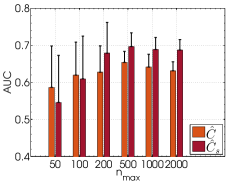
Fig. 2: ROC and corresponding AUCs in the CEP causality problems dataset for $n_{max}=200$ (thin lines) and $n_{max}=2000$ (thick lines) in every problem.

The best recognition curves for both criteria are given in Fig. 3. It can be noted that in both cases, the ROC and the precision recall curves (PRC) for the proposed $\hat{C}_{s}$ are better than those of $\hat{C}$, and this happens for all decision rates, especially in the false positive rates regime.

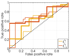
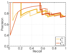
Fig. 3: ROC (left) and Precision-Recall (right) curves for the causality problem using $n=\{50,200,2000\}$ samples (thicker lines mean higher $n$.

5 CONCLUSIONS

We introduced a simple method based on observational data to uncover cause-effect relations in geoscience and remote sensing problems. We relied on a framework based on regression and dependence estimation, and proposed to focus on the sensitivity (curvature) of the dependence estimator instead of the dependence itself. This allows us to better capture the asymmetry of the forward and inverse densities. Results in a large collection of 28 geoscience causal inference problems demonstrated the good performance of our proposal.

References

- [1] Gian-Reto Walther, Eric Post, Peter Convey, Annette Menzel, Camille Parmesan, Trevor J. C. Beebee, Jean-Marc Fromentin, Ove Hoegh-Guldberg, and Franz Bairlein, “Ecological responses to recent climate change,” Nature, vol. 416, no. 6879, pp. 389–395, March 2002.
- [2] David Adam, “Climate change in court,” Nature Clim. Change, vol. 1, no. 10, pp. 1758–678X, 2011.
- [3] Gabriele Hegerl and Francis Zwiers, “Use of models in detection and attribution of climate change: Models in detection and attribution of climate change,” vol. 2, no. 4, pp. 570–591.
- [4] Alessandro Attanasio, Antonello Pasini, and Umberto Triacca, “Granger causality analyses for climatic attribution,” vol. 03, no. 4, pp. 515–522.
- [5] Imme Ebert-Uphoff and Yi Deng, “Causal discovery for climate research using graphical models,” vol. 25, no. 17, pp. 5648–5665.
- [6] Peter Spirtes, Clark Glymour, and Richard Scheines, Causation, prediction, and search, 1993.
- [7] Jakob Runge, Vladimir Petoukhov, Jonathan F. Donges, Jaroslav Hlinka, Nikola Jajcay, Martin Vejmelka, David Hartman, Norbert Marwan, Milan Paluš, and Jürgen Kurths, “Identifying causal gateways and mediators in complex spatio-temporal systems,” vol. 6, pp. 8502.
- [8] P. O. Hoyer, D. Janzing, J. M. Mooij, J. Peters, and B. Schölkopf, “Nonlinear causal discovery with additive noise models,” in NIPS, D. Koller, D. Schuurmans, Y. Bengio, and L. Bottou, Eds., 2008, pp. 689–696.
- [9] A. Gretton, R. Herbrich, and A. Hyvärinen, “Kernel methods for measuring independence,” Journal of Machine Learning Research, vol. 6, pp. 2075–2129, 2005.
- [10] G. Camps-Valls, J. Mooij, and B. Scholkopf, “Remote sensing feature selection by kernel dependence measures,” IEEE Geosc. Rem. Sens. Lett., vol. 7, no. 3, pp. 587 –591, Jul 2010.
- [11] Gustavo Camps-Valls, Devis Tuia, Valero Laparra, and Jesús Malo, “Estimating biophysical variable dependences with kernels,” in IGARSS, 2010, pp. 828–831.
- [12] G. Camps-Valls, J. Verrelst, J. Munoz-Mari, V. Laparra, F. Mateo-Jiménez, and J. Gomez-Dans, “A survey on gaussian processes for earth observation data analysis,” IEEE Geoscience and Remote Sensing Magazine, vol. 4, no. 6, June 2016.
- [13] C. Baker, “Joint measures and cross-covariance operators,” Transactions of the American Mathematical Society, vol. 186, pp. 273–289, 1973.
- [14] Kenji Fukumizu, Francis R. Bach, and Michael I. Jordan, “Dimensionality reduction for supervised learning with reproducing kernel Hilbert spaces,” Journal of Machine Learning Research, vol. 5, pp. 73–99, 2004.
- [15] Arthur Gretton, Olivier Bousquet, Alex Smola, and Bernhard Schölkopf, “Measuring statistical dependence with hilbert-schmidt norms,” in Algorithmic Learning Theory, Sanjay Jain, HansUlrich Simon, and Etsuji Tomita, Eds., vol. 3734 of Lecture Notes in Computer Science, pp. 63–77. Springer Berlin Heidelberg, 2005.
- [16] U. Kjems, L. K. Hansen, J. Anderson, S. Frutiger, S. Muley, J. Sidtis, D. Rottenberg, and S. C. Strother, “The Quantitative Evaluation of Functional Neuroimaging Experiments: Mutual Information Learning Curves,” NeuroImage, vol. 15, no. 4, pp. 772–786, 2002.
- [17] J.E. Burt, G.M. Barber, and D.L. Rigby, Elementary Statistics for Geographers, Guilford Press, 2009.
- [18] Povilas Daniusis, Dominik Janzing, Joris M. Mooij, Jakob Zscheischler, Bastian Steudel, Kun Zhang, and Bernhard Schölkopf, “Inferring deterministic causal relations,” CoRR, vol. abs/1203.3475, 2012.
- [19] Joris M. Mooij, Jonas Peters, Dominik Janzing, Jakob Zscheischler, and Bernhard Schölkopf, “Distinguishing cause from effect using observational data: Methods and benchmarks,” J. Mach. Learn. Res., vol. 17, no. 1, pp. 1103–1204, Jan. 2016.