Simple approaches on how to discover promising strategies for efficient enterprise performance,
at time of crisis in the case of SMEs :
Voronoi clustering and outlier effects perspective

Abstract

This paper analyzes the connection between innovation activities of companies – implemented before a financial crisis – and their performance – measured after such a time of crisis. Pertinent data about companies listed in the STAR Market Segment of the Italian Stock Exchange is analyzed. Innovation is measured through the level of investments in total tangible and intangible fixed assets in 2006-2007, while performance is captured through growth – expressed by variations of sales or of total assets, – profitability – through ROI or ROS evolution, - and productivity – through asset turnover or sales/employee in the period 2008-2010. The variables of interest are analyzed and compared through statistical techniques and by adopting a cluster analysis. In particular, a Voronoi tessellation is implemented in a varying centroids framework. In accord with a large part of the literature, we find that the behavior of the performance of the companies is not univocal when they innovate. The statistical outliers are the best cases in order to suggest efficient strategies. In brief, it is found that a positive rate of investments is preferable.

1 Introduction

This chapter is based on three recent papers :

• (Bartolacci et al., 2015) F. Bartolacci, N.G. Castellano, and R. Cerqueti (2015). The impact of innovation on companies’ performance: an entropy-based analysis of the STAR Market Segment of Italian Stock Exchange, Technology Analysis and Strategic Management 27, 102-123.

• (Ausloos et al., 2018a) M. Ausloos, F. Bartolacci, N.G. Castellano, and R. Cerqueti (2018). Exploring how innovation strategies at time of crisis influence performance: a cluster analysis perspective, Technology Analysis and Strategic Management 30, 484-497.

• (Ausloos et al., 2018b) M. Ausloos, R. Cerqueti, F. Bartolacci, and N. G Castellano (2018). SME investment best strategies. Outliers for assessing how to optimize performance, Physica A 509, 754-765.

The connection between innovation strategies (usually taken as the investments) of companies if implemented before a financial crisis and their performance measured after crisis time are interesting aspects of small and medium size enterprises (SME) economic life.

In fact, Latham and Braun (2011), in ”Economic recessions, strategy, and performance: a synthesis” claimed that

”Despite the episodic pervasiveness of recessions and their destructive impact on firms, a void exists in the management literature examining the intersection between recessions, strategy, and performance”.

Therefore, it seems worthwhile to reflect on such connections considering practical cases. Thus, we have considered companies listed in the STAR Market Segment of the Italian Stock Exchange in recent times. SME innovation is here below measured through the level of investments in total tangible and intangible fixed assets in [2006-2007], while performance is captured through (i) growth – expressed by variations of sales (DS) and variations of total assets (DA), – (ii) profitability – through returns on investments (ROI) and returns on sales (ROS), – and (iii) productivity – through asset turnover (ATO) or sales per employee (S/E) in the period [2008-2010].

In the Milano STAR market, 71 companies of mid-size are listed, at the time of study: their capitalization value was about between 40 million and 1 billion euros. Since their activity and innovation levels are different from ”industrial companies”, whence since their performance should be measured in a different way, we have removed banks and insurance institutes from our analysis. Thus, in the following, the segment is reduced to 62 SMEs. For completeness, the 62 SMEs at the time of study are given in Table 1.

We discuss a formal method, based on Voronoi tessellation (Voronoi, 1908), yet we depart from the original formulation of Voronoi by introducing a concept of weighted Euclidean distances, hence leading to asymmetry (see formulas (2) and (3) below). In our approach, we a priori define some reference points - so called ”centroids”, each centroid identifying a cluster whose elements are at a distance smaller than that to the other centroids.

For more information, let us mention that the use of Voronoi tessellation can be found in Liu et al. (2009), Yushimito et al. (2012) and Vaz et al. (2014).

Such a cluster analysis is employed to investigate the determinants of innovation and innovation-performance focused on a single industry (Tseng et al., 2008), or on different industries (Pavitt, 1984; Cesaratto and Mangano, 1993; Leiponen and Drejer, 2007).

2 Data

A few notations are to be introduced for easy readability of the following tables and figures:

• TIAXyy represents the level of total intangible assets (excluding goodwill) in year 20yy;

• TTAyy is the level of total tangible assets (excluding properties) in 20yy;

• DSyy stands for sales variations in year 20yy

• DAyy is total assets variations, in year 20yy

• ROIyy means the return on investments in year 20yy

• ROSyy means the return on sales in year 20yy

• ATOyy represents asset turnover, in year 20yy

• S/Eyy stands for sales per employee, in year 20yy

• the lowest TTA value is called TTA1, while the highest TTA is TTA2

• their average is : $<$TTA$>$2 = (1/2) (TTA1 + TTA2)

which in fact, due to the time interval of interest, is equal to (TTA06 + TTA07). Similarly,

• $<$TIAX$>$2 is the average total intangible asset (excluding goodwill) over 2 years: [2006-2007]; ”obviously”, $<$TIAX$>$2 = (1/2) (TIAX1 + TIAX2) = (1/2) (TIAX06 + TIAX07).

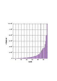
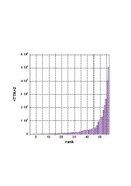
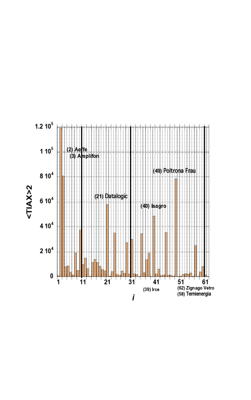
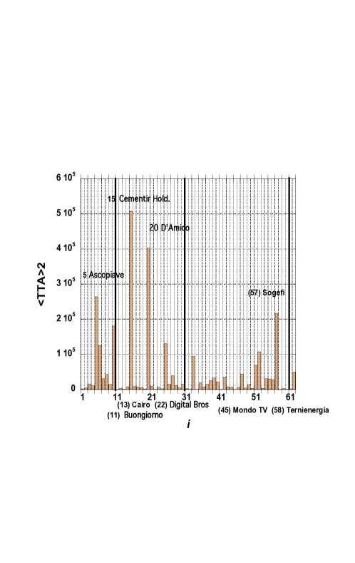
We provide figures in order to visualize the data range for $<$TIAX$>$2 and $<$TTA$>$2. on Fig. 1. In these figures, the SMEs are ranked in increasing order of the $y$-variable value. The range and statistical characteristics are outlined in Table 2. Other displays, e.g., when the SMEs are listed in alphabetical order, on the $x$-axis can be found in Fig. 2.

Figure 1: Left panel: $<$TIAX$>$2. Right panel: $<$TTA$>$2; thus each averaged over 2 years: [2006-2007]; both data are ranked in increasing order, - for the 62 SMEs discussed in the text.

Figure 2: (color online) Left panel: $<$TIAX$>$2. Right panel: $<$TTA$>$2; thus each averaged over 2 years: [2006-2007], - for the 62 SMEs, ranked in alphabetical order as in Table 1, particularly pointing to a few relevant SMEs of the STAR market so studied.

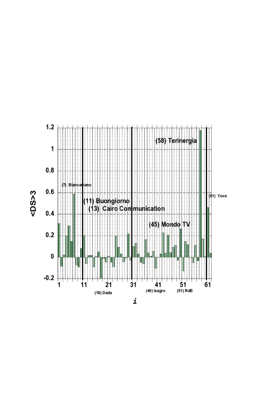
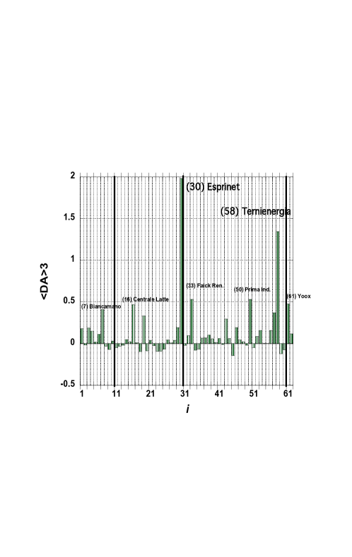
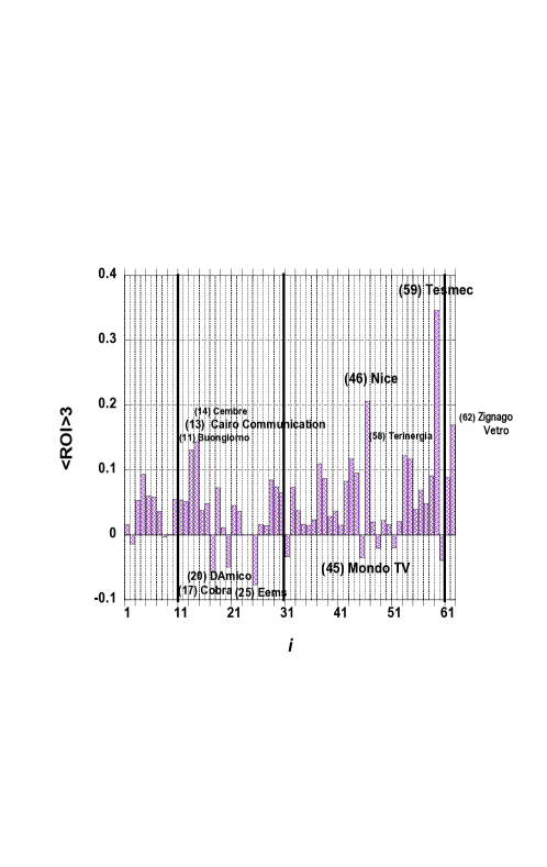
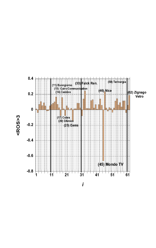
Next, let us display the performance variables averaged over 3 years, [2008-2010]:

• $<$DS$>$3 for the sales variations,

• $<$DA$>$3 for the total assets variations,

• $<$ROI$>$3 for ROI,

• $<$ROS$>$3 for ROS,

• $<$ATO$>$3 for the asset turnovers,

• $<$S/E$>$3 for the sales per employee,

either when companies are listed in alphabetical order, as in Figs. 3-5, or ranked in increasing order of the relevant variable, as in Figs. 6-8.

Figure 3: (color online) Left panel: sales variations $<$DS$>$3. Right panel: total assets variations $<$DA$>$3; thus each averaged over 3 years: [2008-2010], - for the 62 SMEs , ranked in alphabetical order as in Table 1, particularly pointing to a few relevant SMEs of the STAR market so studied.

Figure 4: (color online) Left panel: returns on investments $<$ROI$>$3. Right panel: returns on sales $<$ROS$>$3. Thus each averaged over 3 years: [2008-2010], - for the 62 SMEs , ranked in alphabetical order as in Table 1, particularly pointing to a few relevant SMEs of the STAR market so studied.

Figure 5: (color online) Left panel: asset turnovers $<$ATO$>$3. Right panel: sales per employee $<$S/E$>$3. Thus each averaged over 3 years: [2008-2010], - for the 62 SMEs , ranked in alphabetical order as in Table 11, particularly pointing to a few relevant SMEs of the STAR market so studied

Figure 6: (color online) Left panel: sales variations $<$DS$>$3. Right panel: total assets variations $<$DA$>$3; both ranked in increasing order, - for the 62 SMEs, particularly pointing to a few relevant SMEs of the STAR market so studied.

Figure 7: (color online) Left panel: returns on investments $<$ROI$>$3. Right panel: returns on sales $<$ROS$>$3; both ranked in increasing order, - for the 62 SMEs, particularly pointing to a few relevant SMEs of the STAR market so studied.

Figure 8: (color online) Left panel: asset turnovers $<$ATO$>$3. Right panel: sales per employee $<$S/E$>$3; both ranked in increasing order, - for the 62 SMEs, particularly pointing to a few relevant SMEs of the STAR market so studied.

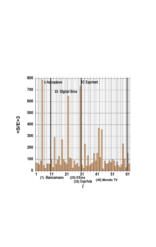
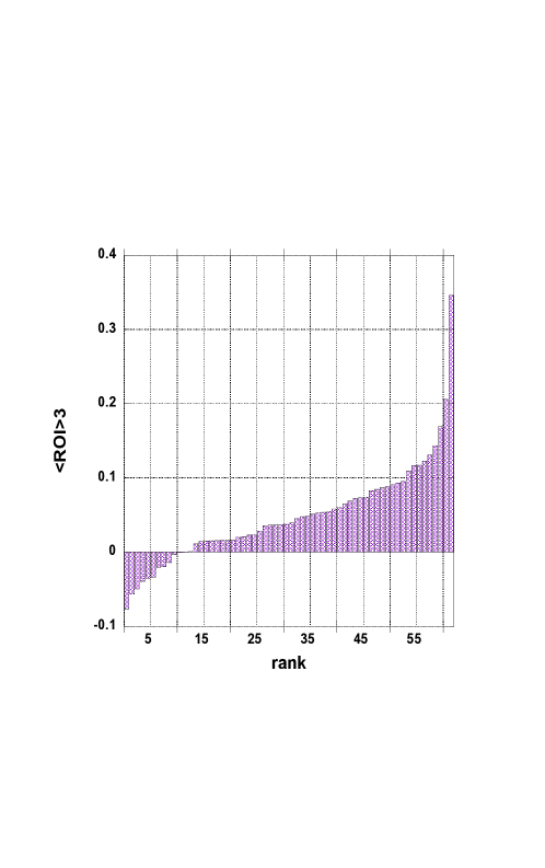
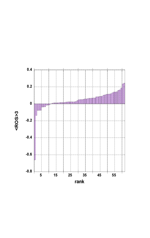
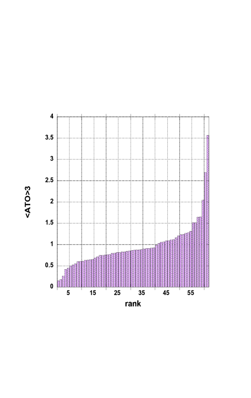
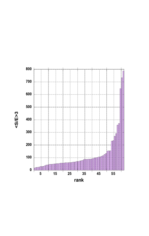
Statistical characteristics for the distributions of the averaged innovation and performance indicators are found in Table 3.

Figure 9: Power law regression analysis for (color online) left panel: TIAX07 vs. TIAX06 and right panel: TTA07 vs. TTA06, for the 62 SMEs.

3 Discussion

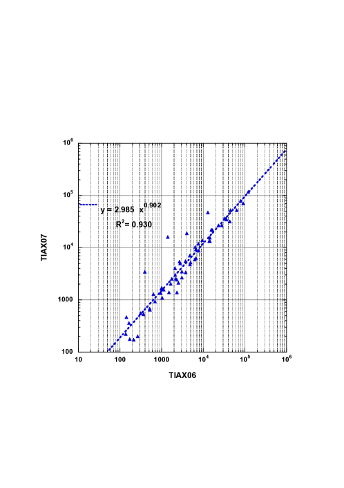
Many correlations can be searched for; beside those between TTA06 and TTA07, or TIAX06 and TIAX07, shown on Fig. 9, one may consider those between the averaged variables, like

• $<$DS$>$3 vs. $<$TTA$>$2

• $<$DA$>$3 vs. $<$TTA$>$2

• $<$ROI$>$3 vs. $<$TTA$>$2

• $<$ROS$>$3 vs. $<$TTA$>$2

which can be read in Figs. 8-11, in Ausloos et al. (2018b), whence are not reproduced here. Nevertheless, for completeness, we show

• $<$ATO$>$3 vs. $<$TIAX$>$2

• $<$S/E$>$3 vs. $<$TIAX$>$2

• $<$ATO$>$3 vs. $<$TTA$>$2

• $<$S/E$>$3 vs. $<$TTA$>$2

on Fig. 10 and Fig. 11.

Figure 10: Searching for correlations: (color online) left panel: $<$ATO$>$3 vs. $<$TIAX$>$2; right panel: $<$S/E$>$3 vs. $<$TIAX$>$2.

Figure 11: Searching for correlations: (color online) left panel: $<$ATO$>$3 vs. $<$TTA$>$2; right panel: $<$S/E$>$3 vs. $<$TTA$>$2.

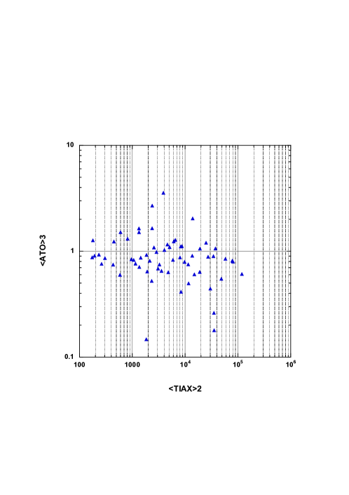
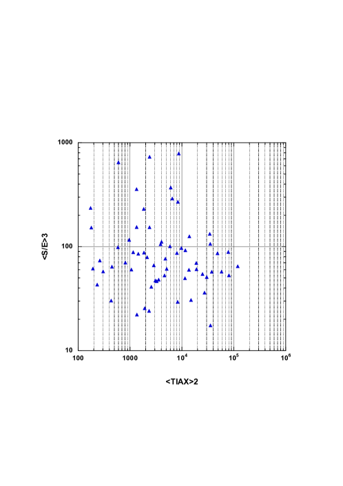
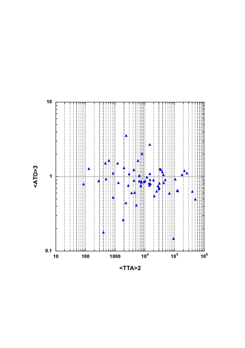
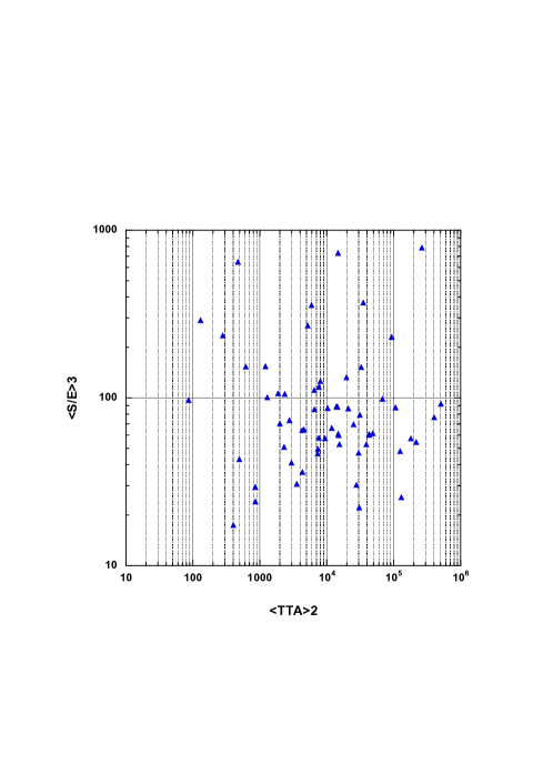
It should be apparent that the data looks pretty scattered, suggesting a ”more sophisticated” approach for reaching some conclusion. As an intermediary remark, observe that $<$ATO$>$3 and $<$S/E$>$3 are all positive; this is not the case for $<$DS$>$3, $<$DA$>$3, $<$ROI$>$3, and $<$ROS$>$3; some SMEs have negative values in the latter cases; see Fig. 6 and on Fig. 7, for examples.

3.1 A brief description of the Voronoi tessellation

The Voronoi tessellation is a method for decomposing a metric space in non-overlapping subsets. Such a methodology dates back to René Descartes, who informally described it in his Principia Philosophiae (Descartes, 1644). Later, it was formalized in the context of the multidimensional real spaces (Voronoi, 1908). The principles behind the conceptualization of the Voronoi tessellation are grounded on the criterion used for decomposing the space. Some specific points – the so-called ”centroids” or ”seeds” – are initially selected. In our context, we refer to a finite number of centroids. Then, the space is partitioned into regions, according to the distances from the seeds. Specifically, each point of the space is assigned to the peculiar centroid which is closer to it. In so doing, the points assigned to a given centroid form a region which contains the centroid itself and does not overlap with other regions/centroids. When all the points of the space are assigned to a specific centroid, then the space appears visually as ”tesselled”; this intuitively suggests why one refers to the ”Voronoi tessellation”. The distance employed for the tessellation procedure can be selected in a number of ways, and it is based on the metric. Here and in most applications , – and also in the original Voronoi’s paper, the considered metric space is the multidimensional Euclidean space. Thus, the natural Voronoi distance is the Euclidean one.

In the present application, we refer to bidimensional Euclidean spaces; the coordinates of the considered points and centroids are $x$ and $y$ variables.

3.2 Voronoi correlations approach

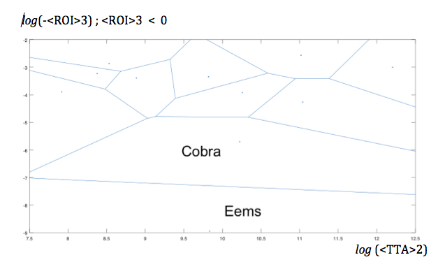
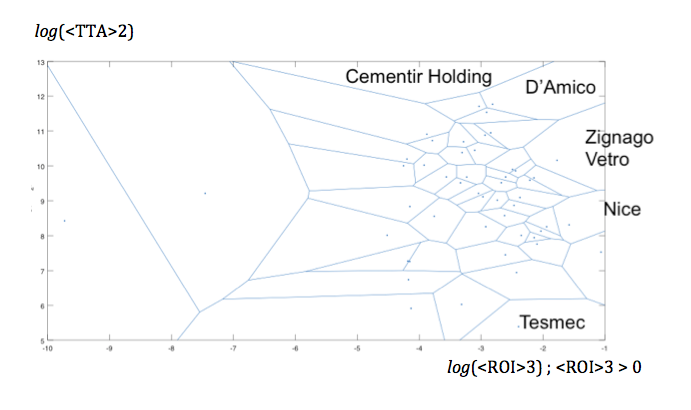
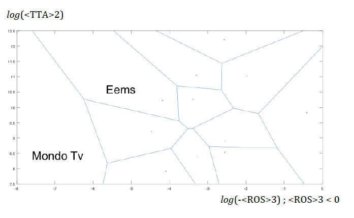
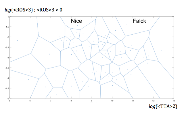
In the context of Voronoi tessellation of the bidimensional Euclidean space, the $x$ and $y$ axes correspond thereafter to one of the innovation ($\mathcal{I}$) and one of the performance ($\mathcal{P}$) variables respectively. It is easily understood that counting only correlations between ($\mathcal{I}$) and performance ($\mathcal{P}$) variables, one has 12 displays; the more so if one considers the log of the variables for display readability (”scaling”), since as pointed out the absolute value of several ($\mathcal{P}$) variables has to be taken before log-scaling, leading to 20 Voronoi maps. This seems to be fine for completeness, but too much for illustrating the purpose and its pedagogical approach at this time. Thus, only a few cases are illustrated thereafter: Figs. 12 -13, for the relationship between $<$TTA$>$2 and $<$ROI$>$3 or $<$ROS$>$3. For readability, the $x$ and $y$ axes differ (are flipped) depending on the figure panel. However, this allows to observe the size of the extreme regions, in which, in some sense, the whole market is divided.

Figure 12: Voronoi tessellation of [log($<$ROI$>$3), log($<$TTA$>$2)] plane. Left panel: when $<$ROI$>$3 $<$ 0. Right panel: when $<$ROI$>$3 $>$ 0 for the 62 SMEs discussed in the text. A few specific SMEs are pointed out.

Figure 13: Voronoi tessellation of [log($<$ROS$>$3), log($<$TTA$>$2)] plane. Left panel: when $<$ROS$>$3 $<0$; Right panel: when $<$ROS$>$3 $>0$ for the 62 SMEs discussed in the text. A few specific SMEs are pointed out.

3.3 Voronoi clustering approach

In the Voronoi clustering approach, for avoiding scale effect, the variables of interest are first normalized. For each company $j=1,\dots,62$, we define:

$$\bar{x}_{j}=\frac{x_{j}-m_{x}}{M_{x}-m_{x}},$$ (1)

where $x_{j}$ represents the value of the variable $x$ for the $j$-th company and

$$m_{x}=\min\limits_{j=1,\dots,62}x_{j},\qquad M_{x}=\max\limits_{j=1,\dots,62}x_{j}.$$

Next, in search of clusters, the centroids of the Voronoi tessellation are a priori defined by positive numbers, $\{\phi_{h}\}_{h=1}^{H}$ and $\{\psi_{k}\}_{k=1}^{K}$, where $H$ and $K$ are a priori chosen integers.

Moreover, we introduce a weighted Euclidean distance, for each innovation variable ($\mathcal{I}$), through

$$d_{\mathcal{I}}(j,\phi_{h})=\sum_{x\in\mathcal{I}}\alpha_{x}(\bar{x}_{j}-\phi_{h})^{2},$$ (2)

for each centroid $\phi_{h}$ and where the $\alpha$’s are the nonnegative weights of the norm, which can differ depending on the centroid, but so that

$$\sum_{x\in\mathcal{I}}\alpha_{x}=1.$$

Analogously, for each performance variable ($\mathcal{P}$), we define:

$$d_{\mathcal{P}}(j,\psi_{k})=\sum_{x\in\mathcal{P}}\beta_{x}(\bar{x}_{j}-\psi_{h})^{2},$$ (3)

for each centroid $\psi_{k}$, imposing

$$\sum_{x\in\mathcal{P}}\beta_{x}=1.$$

In so doing, all distances are $0\leq d_{\mathcal{I}}(j,\phi_{h}),d_{\mathcal{P}}(j,\psi_{k})\leq 1$, for each company $j$ with respect to centroid of coordinates ($\phi_{h}$, $\psi_{k}$).

Notice that, even if Eq. (2) and Eq. (3) look mathematically identical, we prefer to write down both formulas in order to point out that the differences may occur between the sets $\mathcal{I}$ and $\mathcal{P}$ and the related centroids coordinates. Indeed, as we will see below, the definition of the coordinates $\phi$’s and $\psi$’s and the different cardinalities of $\mathcal{I}$ and $\mathcal{P}$ lead to very different settings emphasized in the cases concerning Eq. (2) and Eq. (3).

Three cases of clustering search have been examined in (Ausloos et al., 2108a), always setting $H=K=4$, with the centroids regularly distributed on the plane diagonal: $\{\phi_{h}\}_{h=1}^{H}=\{\psi_{k}\}_{k=1}^{K}=\{1/5,2/5,3/5,4/5\}$. Consider case [$II$], for discussion, when $\alpha_{x}=1/2$ for each $x\in\mathcal{I}$ and an identical weight for the $x\in\mathcal{P}$ variables, i.e., $\beta_{x}=1/7$. This is a ”uniform in value” case, where the definition of the centroids is made by considering a uniform decomposition of the interval $[0,1]$ and all the variables are assumed to equally concur in the Voronoi distance.

It should be pointed out here that after some simple clustering analysis, so called case [$I$], in Ausloos et al. (2018a), 9 companies are controlling the clustering, and collapsing the whole sample into one single cluster, due to their ”outlier aspect” They are : (2) Aeffe, (5) Ascopiave, (15) Cementir Holding, (20) D’Amico, (22) Digital Bros, (30) Esprinet, (45) Mondo Tv, (58) Ternienergia, (59) Tesmec. This numerically confirms the few outlined cases seen in the above figures. These 9 companies are removed for the subsequent Voronoi clustering analysis approach. It remains therefore 53 companies to be examined.

To provide comments on the following results, we call first cluster the one associated with the $\{\phi_{h}\}_{h=1}^{H}=\{\psi_{k}\}_{k=1}^{K}=\{1/5\}$ centroid and, in an increasing way, the second and the third cluster, so that the fourth cluster is the one associated to the values $\{\phi_{h}\}_{h=1}^{H}=\{\psi_{k}\}_{k=1}^{K}=\{4/5\}$.

In Table 5, a description of the clusters of the sample companies is provided.

Referring to innovation clustering, the greatest number of companies (45 out of 53) is located in the first cluster, meaning that, in relative terms, companies undertake low value innovation initiatives (at least those which produce reflections on tangible and intangible assets). Total sales and total assets, which are measures largely employed in literature for company size, show that the higher the intensity of innovation, the higher the size, or conversely. Also the incidence of both tangible and intangible assets (as percentage of the total assets) is increasing in the three innovation clusters, meaning that in highly innovative companies, tangible and intangible assets represent a relevant portion of the disclosed total assets. The mean/std. dev. ratio shows that the composition of the clusters is rather heterogeneous except for the 3rd innovation cluster which is composed by companies whose size is fairly concentrated around the mean. For what concern performance, the distribution of companies among the clusters is quite different from that of innovation.

This provides evidence that the association between innovation and performance is not self-evident. The averages in the performance clusters also do not allow to appraise significant differences neither in terms of company size or incidence of tangible and intangible assets.

Table 6 shows the averages of innovation and performance drivers for the entire sample and so called clustering $II$ analysis approach (Ausloos et al., 2018a) for innovation and performance.

For completeness, we reproduce comments from such a publication. In the first cluster, the averages of innovation for tangible and intangible assets are below the general averages of the entire sample, whereas all performance indicators are above the full sample averages. In the second cluster, a general under-the-general-average performance is associated to an above-the-general-average innovation. In the third cluster, the performance averages are mixed: some of them are above the mean, while the others are below.

Specifically, the $\mu/\sigma$ ratio points that the clusters homogeneity is rather low, meaning that extremely different companies lie within the same cluster both from innovation or performance perspective. The only exception is represented by ATO, since the $\sigma$ is remarkably concentrated around the average $\mu$. This could be interpreted as a possible association between innovation and asset turnover. However, its direction remains unclear, since a high ATO is associated to a low innovation in the first cluster, whereas a low ATO is associated to a medium innovation in the second cluster, while high ATO is associated to high innovation in the third cluster.

It is worth noticing that in the third cluster, companies appear rather homogeneous in terms of performance, particularly for profitability (both ROI and ROS) and efficiency (ATO and S/E). One can argue that, above a particular ”threshold of innovation intensity”, the level performances seems rather homogeneous.

Indeed, similar considerations can be made for performance clustering: the performance averages gradually increase from the first to the third cluster, whereas innovation averages decrease (TIAX) or fluctuate (TTA). The relation innovation-performance seems, then, quite puzzling. Even for performance clustering, heterogeneity generally occurs within the clusters except for ATO.

3.4 Evidence from outliers approach

Since there is a negative minimum for each DS, DA, ROI and ROS, one may guess that some board innovation strategies were rather failures. One observes also some outliers from simple Voronoi analysis; see case ”Clustering I” in Ausloos et al. (2018a). From Table 2, one observes that the kurtosis is always positive and large, indicating lesser chances of extreme negative outcomes. The skewness is also positive, indicating a long upper tail (many small losses and a few extreme gains), and a long lower range tail (many small gains and several extreme losses).

The performance efficiency ratios of the (62) companies, taken one by one, one observes several outliers, i.e. when the SME efficiency value fall outside the relevant $]$$\mu-2\sigma$, $\mu+2\sigma$$[$ interval. There are 3 SMEs which are positive outliers: (58) Terrienergia, (11) Buongiorno, (13) Cairo Communications, and 1 SME which is systematically a ”negative outlier”: (45) Mondo TV, confirming the Voronoi analysis of ”Clustering I”.

It should occur to the reader that those 4 companies are those with very low TTA. Moreover, Mondo TV is the only one among the outliers which has a TTA06 lower than its TTA07, - this SME had about a 50% decrease in investment before the crisis. In contrast, Terrienergia, Buongiorno, and Cairo Communications have a relatively high TTA increase.

One can observe respectively from Fig. 12 and Fig. 13, for example; see also Figs. 5-6 in Ausloos et al. (2018b).

• the relationship between $<$ROI$>$3 and $<$TTA$>$2: a weak $<$ROI$>$3 for Cementir Holding and Ascopiave; a negative but with a large absolute value occurs for D’Amico; in contrast, a large $<$ROI$>$3 occurs for Tesmec, while the negatively largest $<$ROI$>$3 is for Eems, - both firms have a rather low $<$TTA$>$2;

• the relationship between $<$ROS$>$3 and $<$TTA$>$2 indicates a moderate $<$ROS$>$3 positive effect for Sogefi, Ascopiave, D’Amico and Cementir Holding, the four largest TTA companies, ”imposing” a single cluster in the ”Clustering I” Voronoi analysis; a large negative $<$ROS$>$3 effect occurs for Mondo TV; on the other side, the most positive $<$ROS$>$3 is for Falck Renewables, Zignago Vetro, and Nice.

Observe that these companies cover various sectors of activity. Nevertheless, there are differences: Terrienergia and Cairo Communications have very dissimilar performance efficiency behaviors, the former performing better for ”growth”, the latter for ”profitability”. Since Terrienergia, Buongiorno, and Cairo Communications have a high increase in TTA, one might reach some advice concerning innovation strategy. Let TTA increase for better performance.

As an a posteriori” analysis ”proof”, observe that Mondo TV did not increase its TTA, TTA07$<$TTA06, pointing to a deficient strategy. This is pointing to the timing of ”investment” relevance, - not fully clear from the Voronoi analysis. Moreover, observe that the average values are not the critical quantities.

4 Conclusions

Justifying an investment is superb challenge for board members., - the more so at financial crisis time. Payback is unsure; one needs criteria for obtaining efficiency (performance) measures, whence modeling strategies and forecasting. Usually one demands that the level of investments be low and the returns be high. We have here proposed a set of measures for such ”research questions”. We have outlined means for finding correlations and looked for clustering of performance ratios, whence the specific companies ”obeying” strategies based on such ratios. But from the Voronoi clustering approach, it is not obvious that high innovation leads to high performance.

We have found that the timing of investment is very relevant from observing outliers, with either positive or negative results. Extreme values show best strategies !

The Voronoi approach is nevertheless of interest: Within the clusters, one can compare the characteristics and performance of companies holding the same innovation model, whereas between the clusters high heterogeneity should occur assuming that different innovation models might be suitable for different company profile and/or could be associated to different level of performance.

In this respect, cluster analysis seems to be particularly effective in providing a global analysis of the relationship between innovation and performance. Notice that the study allows three considerations from extreme value analysis: not only the investment evolution; up or down, low or high, but also through their average, serving as a control kind of test. It should be obvious that the best performance should be better appreciated when (unexpectedly?) the investment is low, but regularly implemented.

$i=$		Supersector	$i=$		Supersector
1	Acotel Group	Telecommunications	32	Exprivia	Technology
2	Aeffe	P&HG	33	Falck Renewables	Utilities
3	Amplifon	Health Care	34	Fidia	IG&S
4	Ansaldo Sts	IG&S	35	Fiera Milano	IG&S
5	Ascopiave	Utilities	36	Gefran	IG&S
6	Astaldi	C&M	37	I.M.A	IG&S
7	Biancamano	IG&S	38	Interpump Group	IG&S
8	Biesse	IG&S	39	Irce	IG&S
9	Bolzoni	A&P	40	Isagro	Chemicals
10	Brembo	A&P	41	It Way	Technology
11	Buongiorno *	Technology	42	La Doria	F&B
12	Cad It	Technology	43	Landi Renzo	A&P
13	Cairo Communic.	Media	44	Marr	Retail
14	Cembre	IG&S	45	Mondo Tv	Media
15	Cementir Holding	C&M	46	Nice	IG&S
16	Centrale Latte To	F&B	47	Panariagroup	C&M
17	Cobra	Automobiles and Parts	48	Poligraf. S. F	IG&S
18	Dada	Technology	49	Poltrona Frau	P&HG
19	Damiani	Retail	50	Prima Industrie	IG&S
20	D’Amico	IG&S	51	Rdb	C&M
21	Datalogic	IG&S	52	Reno De Medici	IG&S
22	Digital Bros	P&HG	53	Reply	Technology
23	Dmail Group	Media	54	Sabaf	IG&S
24	Dmt	Technology	55	Saes Getters	IG&S
25	Eems **	Technology	56	Servizi Italia	IG&S
26	El.En	IG&S	57	Sogefi	A&P
27	Elica	IG&S	58	Ternienergia	Utilities
28	Emak	P&HG	59	Tesmec	IG&S
29	Engineering	Technology	60	Txt E-Solutions	Technology
30	Esprinet	Technology	61	Yoox	Retail ***
31	Eurotech	Technology	62	Zignago Vetro	IG&S
* Since July 2012, Buongiorno is part of Docomo Digital
** Eems was moved away from Technology in STAR to MTA Market/Segment
*** In March 2015, Yoox merged with Net-a-Porter

Table 1: The 62 STAR company names, at the time of study; alphabetical order and the ”supersector” to which they belog; ”supersector” abbreviations : Automobiles & Parts (A&P); Construction & Materials (C&M); Industrial Goods & Services (IG&S); Personal & Household Goods (P&HG); Food & Beverage (F&B)

References

Agostini, L., Nosella, A., and Soranzo, B. (2015). The impact of formal and informal appropriability regimes on SME profitability in medium high-tech industries. Technology Analysis and Strategic Management 27(4), 405-419.

Archibugi, D. (2001). Pavitt’s taxonomy sixteen years on: a review article, economics of innovation and new technology, Economics of Innovation and New Technology 10(5), 415-425.

Ausloos, M., Bartolacci, F., Castellano, N.G., and Cerqueti, R. (2018). Exploring how innovation strategies at time of crisis influence performance: a cluster analysis perspective, Technology Analysis and Strategic Management, 30(4), 484-497.

Ausloos, M., Cerqueti, R., Bartolacci, F., and Castellano, N.G. (2018). SME investment best strategies. Outliers for assessing how to optimize performance, Physica A 509, 754-765.

Archibugi, D., Filippetti, A., and Frenz, M. (2013). Economic crisis and innovation: Is destruction prevailing over accumulation? Research Policy 42(2), 303-314.

Bartolacci, F., Castellano, N.G., and Cerqueti, R. (2015). The impact of innovation on companies’performance: an entropy-based analysis of the STAR Market Segment of Italian Stock Exchange, Technology Analysis and Strategic Management 27(1), 102-123.

Baum, C.F., Lööf, H., Nabavi, P., and Stephan, A. (2017). A new approach to estimation of the $R\&D$-innovation-productivity relationship. Economics of Innovation and New Technology 26(1/2), 121-133.

Bartolacci, F., Castellano, N.G., and Cerqueti, R. (2015). The impact of innovation on companies’ performance: an entropy-based analysis of the STAR Market Segment of Italian Stock Exchange, Technology Analysis and Strategic Management 27(1), 102-123.

Brusoni, S., Cefis, E., and Orsenigo, L. (2006). Innovate or Die? A critical review of the literature on innovation and performance, CESPRI, Centro di Ricerca sui Processi di Innovazione e Internazionalizzazione, Universitá Commerciale Luigi Bocconi, Working Paper n. 179.

Ceptureanu, E.G., Ceptureanu, S.I., Luchian, C.E., and Luchian. I. (2017). Quality Management in Project Management Consulting. A Case Study in an International Consulting Company. Amfiteatru Economic 19(44), 215-230.

Cesaratto, S., and Mangano, S. (1993). Technological profiles and economic performance in the Italian manufacturing sector. Economics of Innovation and New Technology 2, 237-256.

Chun, D., Chung, Y., and Bang, S. (2015). Impact of firm size and industry type on $R\&D$ efficiency throughout innovation and commercialisation stages: evidence from Korean manufacturing firms. Technology Analysis and Strategic Management 27(8), 895-909.

Cooper, R.G. (1984). The strategy-performance link in product innovation. R& D Management 14(4), 247-259.

De Jong, J.P.J., and Marsili, O. (2006). The fruit flies of innovations: A taxonomy of innovative small firms. Research Policy 35(2), 213-229.

Descartes, R. (1644). Principia Philosophiae. Ludovicus Elzevirius, Amsterdam, 1644

Duyckaerts, C., and Godefroy, G. (2000). Voronoi tessellation to study the numerical density and the spatial distribution of neurones. Journal of Chemical Neuroanatomy 20(1), 83-92.

Dwyer, L., and Mellor, R. (1993). Product innovation strategies and performance of Australian firms. Australian Journal of Management 18(2), 159-180.

Filippetti, A., and Archibugi, D. (2011). Innovation in times of crisis: National Systems of Innovation, structure, and demand. Research Policy 40(2), 179-192.

Gadomski, A. and Kruszewska, N. (2012). On clean grain-boundaries involving growth of nonequilibrium crystalline-amorphous superconducting materials addressed by a phenomenological viewpoint. The European Physical Journal B 85(12), 1-8.

Gligor, M., and Ausloos, M. (2007). Cluster structure of EU-15 countries derived from the correlation matrix analysis of macroeconomic index fluctuations, The European Physical Journal B 57, 139-146.

Gligor, M., and Ausloos, M. (2008a). Convergence and cluster structures in EU area according to fluctuations in macroeconomic indices, Journal of Economic Integration 23, 297-330.

Gligor, M., and Ausloos, M. (2008b). Clusters in weighted macroeconomic networks: the EU case. Introducing the overlapping index of GDP/capita fluctuation correlations, The European Physical Journal B 63, 533-539.

Gocer, I., Alatas, S., and Peker, O. (2016). Effects of $R\&D$ and innovation on income in EU countries: new generation panel cointegration and causality analysis. Theoretical and Applied Economics 23(4), 153-164.

Heirman, A., and Clarysse, B. (2007). Which tangible and intangible assets matter for innovation speed in start-ups? Journal of Product Innovation Management 24(4), 303-315.

Hitt, M.A., Hoskisson, R.E., and Kim, H. (1997). International diversification: effects on innovation and firm performance in product diversified firms. Academy of Management Journal 40(4), 767-798.

Hollenstein, H. (2003). Innovation modes in the Swiss service sector: a cluster analysis based on firm-level data. Research Policy 32, 845-863.

Jensen, M.B., Johnson, B., Lorenz, E., and Lundvall, B.A. (2007). Forms of knowledge and modes of innovation. Research Policy 36, 680-693.

Khan, A.M., and Manopichetwattana, V. (1989). Innovative and non-innovative small firms: types and characteristics. Management Science 15(5), 597-606.

Kirner, E., Kinkel, S., and Jaeger, A. (2009). Innovation paths and the innovation performance of low-technology firms - An empirical analysis of German industry. Research Policy 38, 447-458.

Latham, S. and Braun, M. (2011). Economic recessions, strategy, and performance: a synthesis Journal of Strategy and Management 4 (2), 96-115.

Lawless, M.W. and Anderson, P.C. (1996). Generational technological change: effects of innovation and local rivalry on performance. Academy of Management Journal 39(5), 1185-1217.

Leiponen, A. and Drejer, I. (2007). What exactly are technological regimes? Intra-industry heterogeneity in the organization of innovation activities. Research Policy 36, 1221-1238.

Liu, X.T., Zheng, X.Q., and Li, D.B. (2009). Voronoi Diagram-Based Research on Spatial Distribution Characteristics of Rural Settlements and Its Affecting Factors. A Case Study of Changping District, Beijing [J]. Journal of Ecology and Rural Environment 2, 007.

Montresor, S. and Vezzani, A. (2016). Intangible investments and innovation propensity: Evidence from the Innobarometer 2013. Industry and Innovation 23(4), 331-352.

Nunes, S. and Lopes, R. (2015). Firm performance, innovation modes and territorial embeddedness, European Planning Studies 23(9), 1796-1826.

OECD, (2005). Annual Report, Paris: OECD Publishing.

OECD, (2009). Annual Report, Paris: OECD Publishing.

Park, N.K., Park, U.D., and Lee, J. (2012). Do the Performances of Innovative Firms Differ Depending on Market-oriented or Technology-oriented Strategies?. Industry and Innovation 19(5), 391-414.

Pavitt, K. (1984). Sectoral patterns of technical change: towards a taxonomy and a theory. Research Policy, 13, 343-373.

Ramella, M., Boschin, W., Fadda, D., and Nonino, M. (2001). Finding galaxy clusters using Voronoi tessellations. Astronomy & Astrophysics 368(3), 776-786.

Ranga, M. and Etzkowitz, H. (2012). Great expectations: an innovation solution to the contemporary economic crisis. European Planning Studies 20(9), 1429-1438.

Renzi, A. and Simone, C. (2011). Innovation, tangible and intangible resources: The espace of slacks interaction. Strategic Change 20(1-2), 59-71.

Shin, N., Kraemer, K.L., and Dedrick J. (2017). R&D and firm performance in the semiconductor industry. Industry and Innovation 24(3), 280-297.

Srholec, M. and Verspagen, B. (2012). The Voyage of the Beagle into innovation: Explorations on heterogeneity, selection, and sectors. Industrial and Corporate Change 21(5), 1221-1253.

Sterlacchini A. and Venturini F. (2014). R&D and Productivity in High-Tech Manufacturing: A Comparison between Italy and Spain. Industry and Innovation 21(5), 359-379.

Tseng, C.Y., Hui-Yueh Kuo, H-Y., and Chou, S.S. (2008). Configuration of innovation and performance in the service industry: evidence from the Taiwanese hotel industry. The Service Industries Journal. 28(7), 1015-1028.

Vaz, E., de Noronha Vaz, T., Galindo, P.V., and Nijkamp, P. (2014). Modelling innovation support systems for regional development analysis of cluster structures in innovation in Portugal. Entrepreneurship and Regional Development 26(1-2), 23-46.

Voronoi, G.F. (1908). Nouvelles applications des paramétres continus de la théorie de formes quadratiques, Journal für die reine und angewandte Mathematik 134, 198-287.

Yushimito, W.F., Jaller, M., and Ukkusuri, S. (2012). A Voronoi-based heuristic algorithm for locating distribution centers in disasters. Networks and Spatial Economics 12(1), 21-39.

Zahra, S.A. and Covin, J.G. (1994). Domestic and international competitive focus, technology strategy and company performance: an empirical analysis. Technology Analysis and Strategic Management 6(1), 39-54.

	Innovation		Performance
			Growth		Profitability		Efficiency
	Intangible	Tangible	Sales	$Tot.Ass.$	$Ret.on$	$Ret.on$	Asset	Sales/
	Assets	Assets	$Var.n$	$Var.n$	Invest.	Sales	turnover	$empl.$
	(TIAX)	(TTA)	(DS)	(DA)	(ROI)	(ROS)	(ATO)	(S/E)
mean ($\mu$)	12,360.46	29,215.40	9%	6%	5%	5%	0,91	275.77
Std.Dev.($\sigma$)	18,695.11	45,379.80	16%	14%	5%	7%	0,34	231.20
$\mu/\sigma$	0.66	0.64	0,46	0,57	0,85	0,75	2,68	1.19
min.	180	86.50	-19%	-10%	-8%	-14%	0,15	57.20
Max	80,816	217,237.50	59%	53%	21%	24%	2,04	1,100.76
Q1	1,346.50	3,579.50	-1%	-2%	2%	1%	0,75	148.02
median	3,584	10,329.00	3%	4%	4%	5%	0,86	188.04
Q3	13,917	31,331.50	12%	16%	8%	9%	1,09	281.07
Skewness	2.28	2.57	1.48	1.32	0.44	0.27	0.78	2.25
Kurtosis	5.14	6.79	3.60	1.07	0.60	0.76	1.76	5.05

Table 2: Main statistical indicators of the innovation and performance variables; $Tot.Ass.$ = ”Total Assets”; $Var.n$ = ”variation”; $empl.$ = ”employee”; $Ret.on$= returns on .

Variable	Min.	Max.	Sum	Mean	StDev	Skewness	Kurtosis
				($\mu$)	($\sigma$)
$<$TIAX$>$2	174.5	1.192 105	8.421 106	13 583	22 513	2.7259	8.0364
$<$TTA$>$2	86.5	5.075 105	2.746 106	44 297	92 600	3.3967	12.062
$<$DS$>$3	-0.1924	1.1767	4.9303	0.0795	0.198	3.1414	14.013
$<$DA$>$3	-0.1436	1.9818	7.8786	0.1270	0.330	3.8060	16.885
$<$ROI$>$3	-0.0768	0.3457	3.0115	0.0486	0.067	1.5342	5.1206
$<$ROS$>$3	-0.6609	0.2445	2.5316	0.0408	0.118	-3.505	20.046
$<$ATO$>$3	0.1474	3.5673	59.900	0.9661	0.535	2.4625	8.8557
$<$S/E$>$3	17.464	787.69	7739.5	124.83	155.6	2.9856	8.7591

Table 3: Summary of (rounded) statistical characteristics for the time average distributions of the innovation and performance indicators for the 62 STAR companies, in the center of the table, in per cent and in $10^{6}$ Euros, respectively; the skewness and kurtosis are dimensionless scalars.

”II clustering”		Performance
		$1st$ $cl.$	$2nd$ $cl.$	$3rd$ $cl.$	$4th$ $cl.$	Tot.
Innovation	$1st$ $cl.$	16	22	7	0	45
	$2nd$ $cl.$	2	2	0	0	4
	$3rd$ $cl.$	1	3	0	0	4
	$4th$ $cl.$	0	0	0	0	0
Tot.		19	27	7	0	53

Table 4: Distribution of companies among the clusters ($cl.$), either for clustering $II$, as defined in the text and examined in Ausloos et al. (2018a) for 53 STAR companies

			$Tot.Ass.$	Total	Intangible	Tangible
			2006-2007	Sales	Assets on	Assets on
			(€ /1,000)	(€/1,000)	$Tot.Ass.$	$Tot.Ass.$
	N:	Mean	303,053	267,689	5%	10%
	53	Std.Dev.	304,144	261,828	6%	12%
”II clustering” Innovation
		Mean	241,199	210,452	4%	8%
$1st$ $cl.$	45	Std.Dev.	190,099	187,814	5%	8%
		Mean/St.Dev.	1.27	1.12	0.88	1.04
		Mean	731,745	467,442	8%	16%
$2nd$ $cl.$	4	Std.Dev.	798,924	469,023	8%	22%
		Mean/St.Dev.	0.92	1.00	0.97	0.73
		Mean	570,226	711,853	12%	22%
$3rd$ $cl.$	4	Std.Dev.	261,414	329,233	9%	27%
		Mean/St.Dev.	2.18	2.16	1.39	0.82
”II clustering” Performance
		Mean	210,607	157,375	8%	10%
$1st$ $cl.$	19	Std. Dev.	130,310	118,218	7%	11%
		Mean/St.Dev.	1.62	1.33	1.14	0.94
		Mean	385,628	354,434	3%	9%
$2nd$ $cl.$	27	Std.Dev.	387,615	293,834	3%	13%
		Mean/St.Dev.	0.99	1.21	0.90	0.71
		Mean	235,476	232,525	3%	10%
$3rd$ $cl.$	7	Std.Dev.	228,112	340,089	5%	12%
		Mean/St.Dev.	1.03	0.68	0.62	0.85

Table 5: Statistical description of the companies, as if one full sample, or ”belonging” to a cluster $cl.$ (see text); the number (N) of companies in each cluster is given; $Tot.Ass.$ = ”Total Assets”.

	TIAX		TTA	DS	DA	ROI	ROS	ATO	S/E
Ent.	Mean ($\mu$)	12,360	29,215	6%	9%	5%	5%	0.91	275.77
	Std.Dev.($\sigma$)	18,695	45,380	14%	16%	5%	7%	0.34	231.20
N=53	$\mu/\sigma$	0.66	0.64	0.46	0.57	0.85	0.75	2.68	1.19
Innovation II clustering
$1st$	Mean ($\mu$)	7,127	18,554	7%	9%	5%	6%	0.93	293.83
$cl.$	Std.Dev.($\sigma$)	9,311	24,023	15%	17%	6%	7%	0.36	248.53
N=45	$\mu/\sigma$	0.77	0.77	0.49	0.55	0.87	0.79	2.57	1.18
$2nd$	Mean ($\mu$)	28,081	71,512	4%	3%	2%	2%	0.67	165.90
$cl.$	Std.Dev.($\sigma$)	29,505	65,192	11%	7%	6%	10%	0.13	58.91
N=4	$\mu/\sigma$	0.95	1.10	0.34	0.35	0.25	0.16	5.36	2.81
$3rd$	Mean ($\mu$)	55,511	106,862	1%	14%	4%	5%	0.97	182.49
$cl.$	Std.Dev.($\sigma$)	28,454	107,418	5%	18%	1%	2%	0.20	48.84
N=4	$\mu/\sigma$	1.95	0.99	0.19	0.81	3.00	2.57	4.91	3.73
Performance II clustering
$1st$	Mean ($\mu$)	16,356	22,484	-2%	-4%	0%	0%	0.79	222.75
$cl.$	Std.Dev.($\sigma$)	20,762	31,548	10%	4%	4%	7%	0.28	157.65
N=19	$\mu/\sigma$	0.79	0.71	0.21	0.83	0.05	0.05	2.85	1.41
$2nd$	Mean ($\mu$)	11,930	35,841	9%	12%	7%	8%	0.94	262.81
$cl.$	Std.Dev.($\sigma$)	19,346	56,259	9%	13%	4%	5%	0.25	232.07
N=27	$\mu/\sigma$	0.62	0.64	0.94	0.92	1.54	1.46	3.77	1.13
$3rd$	Mean ($\mu$)	3,174	21,931	20%	35%	9%	12%	1.11	469.70
$cl.$	Std.Dev.($\sigma$)	4,744	32,962	24%	17%	6%	9%	0.65	332.70
N=7	$\mu/\sigma$	0.67	0.67	0.84	2.02	1.49	1.26	1.71	1.41

Table 6: Main statistical characteristics of the Innovation and Performance variables for the whole sample (Ent.) or inside the clusters ($cl.$); the number (N) of companies inside each cluster is recalled.