Online Photometric Calibration of
Automatic Gain Thermal Infrared Cameras

Abstract

Thermal infrared cameras are increasingly being used in various applications such as robot vision, industrial inspection and medical imaging, thanks to their improved resolution and portability. However, the performance of traditional computer vision techniques developed for electro-optical imagery does not directly translate to the thermal domain due to two major reasons: these algorithms require photometric assumptions to hold, and methods for photometric calibration of RGB cameras cannot be applied to thermal-infrared cameras due to difference in data acquisition and sensor phenomenology. In this paper, we take a step in this direction, and introduce a novel algorithm for online photometric calibration of thermal-infrared cameras. Our proposed method does not require any specific driver/hardware support and hence can be applied to any commercial off-the-shelf thermal IR camera. We present this in the context of visual odometry and SLAM algorithms, and demonstrate the efficacy of our proposed system through extensive experiments for both standard benchmark datasets, and real-world field tests with a thermal-infrared camera in natural outdoor environments.

I Introduction

In the last decade, tremendous efforts have been devoted towards the development of computer vision methods to autonomous robotic systems. Due to their success, a broad range of critical applications from disaster scene surveillance to autonomous driving and package delivery have been made possible already, or are well within reach. However, most of these approaches have addressed only daytime operation under normal illumination, using standard visible-spectrum cameras. For applications that are not resource-constrained and allow the use of active sensors such as LiDARs for night-time operation, they still do not scale to other visually-degraded environmental effects such as fog, smoke, and dust [1]. This is very limiting, and enabling operations to more challenging conditions would significantly enhance the tactical value of such systems.

In this paper, we argue that thermal infrared (TIR) cameras offer a compelling and complementary advantage to both visible-spectrum cameras and LiDARs. The nature of the TIR modality makes them highly robust to both low-illumination conditions and in the presence of adverse obscurants [2]. Furthermore, due to the rapid growth in sensory technology [3], the quality of images and frame-rate generation of low SWaP, COTS, uncooled micro-bolometer arrays ($\mu$BA) based TIR cameras have increased to a level that is suitable for common computer vision tasks. As a result, there has been a growing interest in the computer vision community to use thermal cameras - ranging from object detection [4] and activity recognition [5] to stereo [6], visual odometry [7, 8], SLAM [9, 10] and 3D mapping [11]. See [12] for a comprehensive review on computer vision research and applications with thermal infrared cameras.

(a)

(b)

(c)

(d)

(e)

(f)

(a)

(b)

(c)

(d)

(e)

(f)

Figure 1: In this paper we propose an approach for full photometric calibration of automatic gain thermal-infrared videos, which can be used either offline for calibrating existing datasets, or online in combination with state-of-the-art VO or SLAM pipelines. Top: Sequence of thermal images from the KAIST dataset [13] with strong exposure changes. Bottom: the same sequence after photometric calibration.

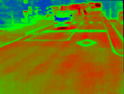
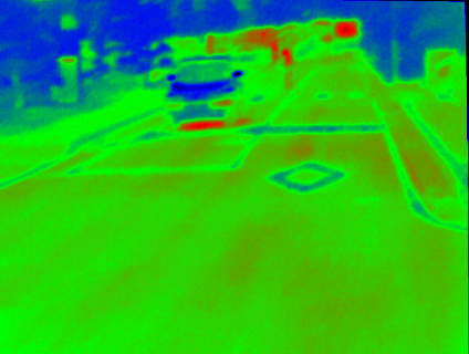
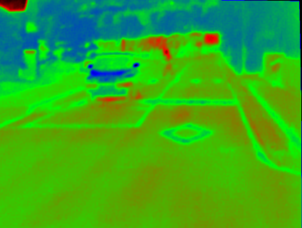
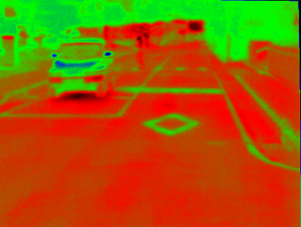
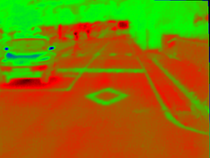
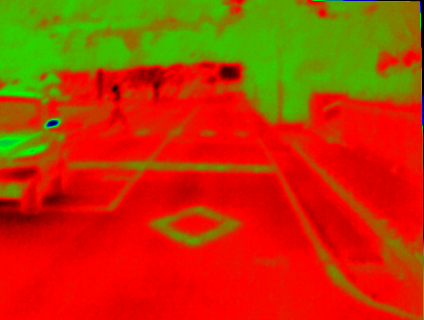
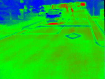
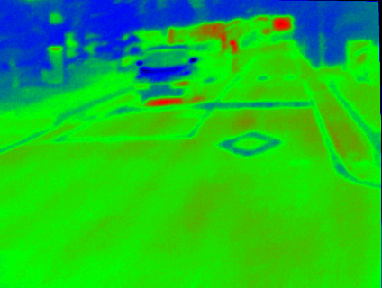
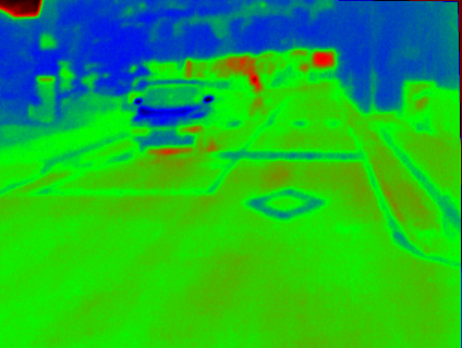
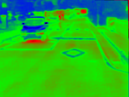
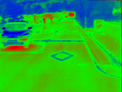
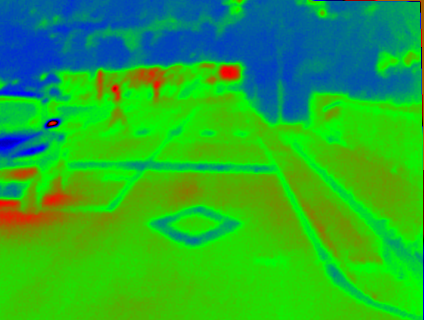
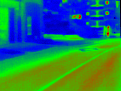
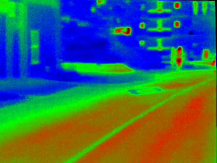
Despite the aforementioned advantages, the performance of traditional computer vision techniques developed for electro-optical imagery does not directly translate to the thermal domain [11, 14]. This is primarily because these cameras have several characteristics that are challenging for vision algorithms. In particular, for visual odometry and SLAM algorithms, one of the biggest challenges is photometric inconsistency due to rapid automatic gain change (AGC). As hot objects move in and out of the camera’s field of view, large regions of pixels saturate, and the sensor adjusts gain to darken the image in an attempt to avoid saturation. The resulting change in intensity can be dramatic from one frame to the next (as shown in Figure 1), invalidating the constant brightness assumption [9] enforced in most low-level computer vision tasks (both direct or feature-based).

It is be noted that the actual measured radiometric values of the objects in the environment are not affected by the observation of other objects. On the contrary, only the appearance of objects in the rescaled thermal images changes as a response to the rescaling operation applied to full radiometric data. One easy fix is to disable AGC completely [15], perform sensor-specific photometric calibration [16] and manually set a fixed thermal range for the entire operation. This requires prior knowledge of the particular environment, and this limits the generalization of methods and applicability to long-term navigation tasks [17]. Furthermore, one might want to run a visual odometry or SLAM algorithm on datasets where no photometric calibration is provided and no access to the camera is given. In these cases, it is necessary to use an algorithm that can provide photometric calibrations for arbitrary video sequences. While such approaches exist for visual spectral cameras [18, 19, 20], the same photometric model cannot be used for TIR cameras due to different data acquisition mechanism, sensor phenomenology and non-uniform properties of the $\mu$BA.

In this paper, our goal was to develop an approach for full photometric calibration of automatic gain TIR cameras, which can be used either offline for calibrating existing datasets, or online in combination with state-of-the-art visual odometry or SLAM pipelines. Specifically, our contributions are threefold: First, we develop a new photometric model that accounts for 1) automatic temporal changes in gains, and 2) spatial biases in pixel intensities of TIR cameras. Second, we present an efficient multi-threaded algorithm that estimated the parameters of the proposed model in real-time by solving multiple non-linear least square problems. Finally, we demonstrate that our proposed calibration approach benefits various downstream computer vision pipelines through extensive experiments with both standard datasets and real-world field tests with a TIR camera.

II Photometric Model for TIR Cameras

A microbolometer is an temperature-dependent electrical resistor (as illustrated in Figure 2a). Infrared radiation with wavelengths between $7.5-14\mu m$ strikes the detector material, heating it, and thus changing its electrical resistance. This resistance change is measured by a readout integrated circuit (ROIC) and processed into temperatures. Many such microbolometers are arranged in a 2D grid to form a focal plane $\mu$BA, where temperature reading from each microbolometer is used to generate intensity for the corresponding pixel in the image.

The infrared energy radiated by an object comprises of the energy emitted, transmitted and reflected by the object. For our photometric model, we assume that the infrared emissivity of an object is invariant to the viewing angle of an observer. While this is true only for a blackbody object, Vollmer et al. [21] upon studying a wide variety of materials observed that for nearly all practically relevant surfaces, the emissivity is nearly constant up to at least $\pm 45^{\circ}$ viewing angle (as illustrated in Figure 2b). Furthermore, outside this range, for a nonconductor dominant scene if our viewing angle does not change much, the emissivity would also not change much until extreme viewing angles $>78^{\circ}$.

(a)

(b)

Figure 2: Left: A generalized cross-sectional view of a $\mu$BA pixel. Right: Emissivity $\varepsilon(\delta)$ as a function of vieweing angle $\delta$ for blackbody, nonconductor and conductor. Source [21]

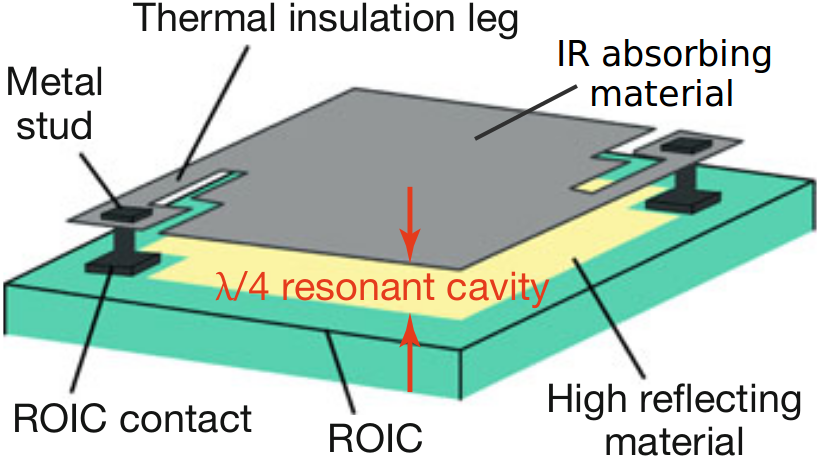
Now consider a 3D world point in the scene which is emitting a constant amount of infrared energy with radiant power $\Phi_{o}$. The change in electrical resistance of the microbolometer is given by Equation 1, where $\alpha\Phi_{o}$ is absorbed radiant power, $\beta$ is thermal coefficient and $G_{\textnormal{th}}$ is total thermal conductance. The change in resistance can also be expressed in terms of the change in temperature $\Delta T$ of the microbolometer as Equation 2 where $\overline{\beta R}$ is the average value in the temperature interval $\Delta T$. Refer to [21] for more details on response generation.

$$\Delta R=\frac{\beta R\alpha\Phi_{o}}{G_{\textnormal{th}}}$$ (1)

$$\Delta R=\overline{\beta R}\Delta T$$ (2)

Now. after simplification, if the microbolometer is sensitive to an energy range given by $[\Phi_{\textnormal{min}},\Phi_{\textnormal{max}}]$, then the normalized response from the sensor is given by $I=(\Phi-\Phi_{\textnormal{min}})/(\Phi_{\textnormal{max}}-\Phi_{\textnormal{min}})$. This response $I$ is used to generate intensity value for the corresponding pixel in the synthetic image $\mathcal{I}:\Omega\rightarrow[0,1]$. Here $\Omega$ denotes the image domain.

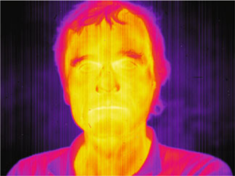
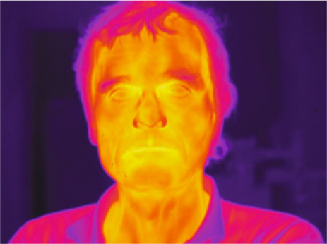
We observe that the image intensity of a scene point with constant thermal radiant energy varies when viewed at a different spatial location in the image $x\in\Omega$. In visible spectrum cameras, this spatially varying image intensity is contributed to radial-lens vignetting (Figure 3a) and modelled as a sixth-order polynomial [19], assuming that the attenuation factors follow a radial model and the center of vignetting coincides with the image center. In regards to TIR cameras, the spatial variation does not take a predefined or symmetric shape (Figure 3b). The variation can be due to two major reasons: 1) the response of each microbolometer might be different either due to the design properties or saturation of the sensor that leads to residuals in their reading, and 2) any infrared transmission effects that lead to uneven transparency including lens effects. The infrared thermal imaging community is well aware of the non-uniform responses by the individual microbolometers in the array. Therefore the non-uniform correction (NUC) (Figure 3c) to correct for the different gains and signal offsets of individual detectors has been widely studied [22, 23, 16]. While most of the hardware will come pre-calibrated, we do not assume the same in our approach to generalize over wide range of cameras. For photometric calibration we are more concerned about low-frequency non-uniformness; variation that spreads across a large area of pixels, and is significant enough to introduce photometric errors. The microbolometers can also get heated by the camera device itself, most commonly due to uneven saturation during operation and the lack of cooling. Therefore the low cost uncooled $\mu$BA-based cameras are more susceptible to low-frequency spatial variations.

We model this effect using an affine sensor response given by $I^{\prime}_{x}=s_{x}(I_{x}+r_{x})$. However, we observe that using only the bias $r_{x}$ and ignoring the scale factor $s_{x}$ is sufficient to model this low-frequency effect while reducing the number of parameters by half. Thus, the spatial bias is modeled by an offset $r_{x}$ in the pixel is given by Equation 3. We also observe that the camera tries to maintain best possible temperature resolution at each time (or frame) $t$ in the image and therefore we can express $I^{\prime}_{x}$ as a normalized value (Equation 4) within a range $[I^{\prime}_{t,\textnormal{min}},I^{\prime}_{t,\textnormal{max}}]$, where $I^{\prime}_{t,\textnormal{min}}$ and $I^{\prime}_{t,\textnormal{max}}$ are the minimum and maximum responses respectively among all the microbolometers for the particular frame $t$.

(a)

(b)

(c)

(d)

Figure 3: Visualization of (a) radial lens vignetting used for visual spectral cameras [18], as compared to (b) non-symmetric spatial variation in $\mu$BA-based TIR camera estimated by our method. TIR images (c) before and (d) after NUC performed by the manufacturer on the hardware (note the streaks) (Source [21]).

$$I^{\prime}_{x}=I_{x}+r_{x}$$ (3)

$$I^{\prime}_{x,t}=\frac{I^{\prime}_{x}-I^{\prime}_{t,\textnormal{min}}}{I^{\prime}_{t,\textnormal{max}}-I^{\prime}_{t,\textnormal{min}}}$$ (4)

Thus, the raw response from the sensor after spatial error is shifted by $I^{\prime}_{t,\textnormal{min}}$ and scaled by $(I^{\prime}_{t,\textnormal{max}}-I^{\prime}_{t,\textnormal{min}})^{-1}$ before being used to generate the image. This is a major contributor to the effect commonly known as gain change or AGC. This implies that the scene point with constant thermal radiant energy may appear with different image intensities in consecutive frames.

Finally, combining Equation 3 and Equation 4, the normalized temperature response is given by Equation 5. In Equation 6 we describe the gain change as an affine brightness response function, similar to [24] for visual spectral images, where $e^{a_{t}}=I^{\prime}_{t,\textnormal{max}}-I^{\prime}_{t,\textnormal{min}}$ and $b_{t}=I^{\prime}_{t,\textnormal{min}}$.

$$I^{\prime}_{x,t}=\frac{I_{x}+r_{x}-I^{\prime}_{t,\textnormal{min}}}{I^{\prime}_{t,\textnormal{max}}-I^{\prime}_{t,\textnormal{min}}}$$ (5)

$$I^{\prime}_{x,t}=\frac{I_{x}+r_{x}-b_{t}}{e^{a_{t}}}$$ (6)

The logarithmic parameterization of the scale factor $e^{-a_{t}}$ prevents it from becoming negative and makes it numerically stable. The goal of the proposed photometric calibration then is to attempt to estimate $a_{t}$ and $b_{t}$ for each frame and $r_{x}$ for each pixel such that, a scene point in the world with constant radiant energy should appear with the same image intensity value invariant to temporal frames and spatial locations.

III Algorithmic Framework

III-A Problem Formulation

Let $p,m,n\in\Omega$ be the pixel locations for the same 3D world point at frames $o,t\text{ and }t+1$ respectively, thus, $I_{p}=I_{m}=I_{n}$. Without loss of generality, consider $o$ to be a hypothetical frame where $e^{a_{o}}=1$, $b_{o}=0$ and without any residual errors, such that $I^{\prime}_{p,o}=I_{p}$. At other frames $t,t+1$, we can consider the parameters be represented with respect to the hypothetical frame $o$. Now using Equation 6

$$I^{\prime}_{m,t} =(I^{\prime}_{p,o}-{}^{o}b_{t}+{}^{p}r_{m})/e^{{}^{o}a_{t}}$$ (7)

$$I^{\prime}_{n,t+1} =(I^{\prime}_{p,o}-{}^{o}b_{t+1}+{}^{p}r_{n})/e^{{}^{o}a_{t+1}}$$

$$=(I^{\prime}_{m,t}e^{{}^{o}a_{t}}+{}^{o}b_{t}-{}^{p}r_{m}-{}^{o}b_{t+1}+{}^{p}r_{n})/e^{{}^{o}a_{t+1}}$$

$$=f_{P}(I^{\prime}_{m,t})$$ (8)

where, $P$ represents the set of model parameters and ${}^{p}r_{m}=r_{m}-r_{p}$. We factor out the intensity $I^{\prime}_{p,o}$ of the hypothetical frame as it is unobservable, and decompose the function $f_{P}(I^{\prime}_{m,t})$ as follows:

$$f_{P}(I^{\prime}_{m,t}) =\frac{I^{\prime}_{m,t}e^{{}^{o}a_{t}}+{}^{o}b_{t}-{}^{o}b_{t+1}}{e^{{}^{o}a_{t+1}}}+\frac{{}^{p}r_{n}-{}^{p}r_{m}}{e^{{}^{o}a_{t+1}}}$$

$$=g_{P_{t}}(I^{\prime}_{m,t})+h_{P_{t},\mathcal{P}_{s}}$$ (9)

where $P=P_{t}\cup\mathcal{P}_{s}$ are the unknown set of parameters that relates to temporal and spatial variations respectively. Thus, there are two unknown parameters ($\{{}^{o}a_{t},{}^{o}b_{t}\}\subset P_{t}$) per frame, and additional $\mathcal{P}_{s}=\mathcal{O}(|\Omega|)$ unknown parameters. Our goal is to estimate these parameters efficiently in a real-time online setting using pixel correspondences across frames (see III-F for details regarding correspondences).

III-B Measurement Model

Let $\epsilon$ be zero-mean Gaussian noise, we consider our measurement model as

$$I^{\prime}_{n,t+1} =g_{P_{t}}(I^{\prime}_{m,t})+h_{P_{t},\mathcal{P}_{s}}+\epsilon$$

$$=g_{P_{t}}(I^{\prime}_{m,t})+\frac{\Delta_{n,m}}{e^{{}^{o}a_{t+1}}}+\epsilon$$

where $\Delta_{n,m}={}^{p}r_{n}-{}^{p}r_{m}$. If we ignore the $h_{P_{t},\mathcal{P}_{s}}$ term, and consider the estimation of only the $P_{t}$ parameters, the Maximum Likelihood Estimate of $P_{t}$ corresponds to the solution of the least squares objective given by

$$\begin{split}O_{\text{T}}(g_{P_{t}},C_{t})=&\min\limits_{P_{t}}\sum_{(m,n)\in C_{t}}\lVert I^{\prime}_{n,t+1}-g_{P_{t}}(I^{\prime}_{m,t})\rVert^{2}\end{split}$$ (10)

where $C_{t}$ denotes the set of pixel correspondences between frame $t$ and $t+1$. Note that, the term $\Delta_{n,m}/e^{{}^{o}a_{t+1}}$ becomes part of the error, however unlike $\epsilon$, it is not zero-mean. Thus, minimizing the objective function Equation 10 favors the minimization of $\Delta_{n,m}/e^{{}^{o}a_{t+1}}$. This has an adverse effect on ${}^{o}a_{t+1}$, as when $\Delta_{n,m}>0$, the term $e^{{}^{o}a_{t+1}}$ gets increased, and vice versa. However, if we do not ignore the $h_{P_{t},\mathcal{P}_{s}}$ term, on one hand, we can prevent the aforementioned bias, but on the other hand, our objective function in Equation 11 includes the additional unknown terms $\mathcal{P}_{s}$

$$\begin{split}O_{\text{TS}}(f_{P_{t},\mathcal{P}_{s}},C_{t})=&\min\limits_{P_{t},\mathcal{P}_{s}}\sum_{t=1}^{N}\sum_{(m,n)\in C_{t}}\lVert I^{\prime}_{n,t+1}-f_{P_{t},\mathcal{P}_{s}}(I^{\prime}_{m,t})\rVert^{2}\end{split}$$ (11)

III-C Estimating Temporal Parameters

There are two unknown temporal parameters (${}^{o}a_{t},{}^{o}b_{t}$) per frame. We desire to update them with minimal computational overhead in order to maintain high frame rate throughput. Using either objective functions Equation 10 or Equation 11, we can iteratively solve for ${}^{o}a_{t},{}^{o}b_{t}$ using ${}^{o}a_{t-1},{}^{o}b_{t-1}$, and point correspondences between frame $(t-1)$ and $t$. If we use the latter, we need to either also estimate $\mathcal{P}_{s}$ or fix them with known values. Alternatively, if we use the former, we face the problem of bias as discussed in III-B. To solve this, we observe that spatial variations occur in small regions on the image, and thus, we assume that majority of the pixel correspondences have $\Delta_{n,m}\approx 0$, while those with $\Delta_{n,m}>>0$ will form the minority. We employ RANSAC [25] to reject the outliers and estimate $P_{t}$.

Next, for any pair ($t,t+1$) of frames in consideration, instead of estimating all the unknown parameters ($\{{}^{o}a_{t},{}^{o}b_{t},{}^{o}a_{t+1},{}^{o}b_{t+1}\}$) w.r.t. the hypothetical frame $o$, we instead estimate the relative parameters ($\{{}^{t}a_{t+1},{}^{t}b_{t+1}\}$) $\displaystyle e^{{}^{t}a_{t+1}}=\frac{e^{{}^{o}a_{t+1}}}{e^{{}^{o}a_{t}}}$ (12) $\displaystyle{}^{t}b_{t+1}=\frac{{}^{o}b_{t+1}-{}^{o}b_{t}}{e^{{}^{o}a_{t}}}$ (13)

$$e^{{}^{t}a_{t+1}} =e^{{}^{t}a_{t+1}}\times e^{{}^{t+1}a_{t+2}}$$ (14)

$${}^{t}b_{t+2} ={}^{t}b_{t+1}+e^{{}^{t}a_{t+1}}\times{}^{t+1}b_{t+2}$$ (15)

Thus, using subsection III-A, Equation 12, Equation 13 and ignoring $h_{P_{t},\mathcal{P}_{s}}$

$$I^{\prime}_{n,t+1}=(I^{\prime}_{m,t}-{}^{t}b_{t+1})/e^{{}^{t}a_{t+1}}=g^{\prime}_{P^{\prime}_{t}}(I^{\prime}_{m,t})$$ (16)

Until now, we considered only consecutive frames ($t,t+1$) in our discussion to indicate a sense of sequential and progressive process. However, in the presence of pixel correspondences $C_{i,j}$, the above concepts would generalize to any two frames $i,j$, and the relative parameters $P^{\prime}_{i,j}=\{{}^{i}a_{j},{}^{i}b_{j}\}$ can be estimated using $O_{\text{T}}(g^{\prime}_{P^{\prime}_{i,j}},C_{i,j})$ in Equation 10. In-fact a current frame $t$ can have pixel correspondences with multiple previous frames $t-1,t-2,t-k,\ldots$, and all of these correspondences are used to get the best estimate for $P^{\prime}_{t-1,t}=\{{}^{t-1}a_{t},{}^{t-1}b_{t}\}$ as described in Alg. 1. Thus, we again overload the notation for $C_{t}=C_{t-1,t}\cup C_{t-2,t}\cup C_{t-k,t}\cup\ldots$ to denote the set that contains all the pixel correspondences from previous frames to the current frame $t$. Despite of having correspondences from multiple previous frames, the estimates ($P^{\prime}_{t-1,t}$) might still incur drift error, hence, in AdjustForDrift, we attempt to keep the parameters close to their nominal values. Finally, let $P^{\prime}_{t-1}=\bigcup^{t-1}_{x=t-N}P^{\prime}_{1,x}$ be the set of all parameters for $N$ frames relative to the first frame, where $P^{\prime}_{1,1}=\{{}^{1}a_{1}=1,{}^{1}b_{1}=0\}$, and for all other frames $x\neq 1$, $P^{\prime}_{1,x}$ is computed by chaining all $P^{\prime}_{y-1,y},y=[2\mathrel{{.}\,{.}}\nobreak x]$ using Equation 14 and Equation 15. We employ multi-threading to run the iterations of the “for” loop in line 4 Alg. 1 as they are independent.

Algorithm 1 Estimating temporal parameters

1:$C_{t}$, $P^{\prime}_{t-1}$, $N$

2:$P^{\prime}_{t}$, the set of all relative parameters upto frame $t$

3:function Main($C_{t},P^{\prime}_{t-1},N$)

4:     $T$ $\leftarrow$ $0$

5:     $\{{}^{t-1}a_{t},{}^{t-1}b_{t}\}$ $\leftarrow$ $\{0,0\}$

6:     for each $C_{i,t}\in C_{t}$ asynchronously in parallel do

7:         $P^{\prime}_{i,t}$ $\leftarrow$ Ransac on Equation 10 using $O_{\text{T}}(g^{\prime}_{P^{\prime}_{i,t}},C_{i,t})$

8:         $a^{i},b^{i}$ $\leftarrow$ ChangeRef($P^{\prime}_{i,t}$, $P^{\prime}_{1,i}$, $P^{\prime}_{1,t-1}$)

9:         ${}^{t-1}a_{t}$ $\leftarrow$ ${}^{t-1}a_{t}+a^{i}\times|C_{i,t}|$

10:         ${}^{t-1}b_{t}$ $\leftarrow$ ${}^{t-1}b_{t}+b^{i}\times|C_{i,t}|$

11:         $T$ $\leftarrow$ $T+|C_{i,j}|$      

12:     $\{{}^{t-1}a_{t},{}^{t-1}b_{t}\}$ $\leftarrow$ $\{{}^{t-1}a_{t}/T,{}^{t-1}b_{t}/T\}$

13:     $\{{}^{t-1}a_{t},{}^{t-1}b_{t}\}$ $\leftarrow$ AdjustForDrift(${}^{t-1}a_{t},{}^{t-1}b_{t}$)

14:     $\{{}^{1}a_{t},{}^{1}b_{t}\}$ $\leftarrow$ $\{{}^{1}a_{t-1}+{}^{t-1}a_{t},{}^{1}b_{i}+e^{{}^{1}a_{t-1}}\times{}^{t-1}b_{t}\}$

15:     $P^{\prime}_{t}$ $\leftarrow$ $P^{\prime}_{t-1}\cup\{\{{}^{1}a_{t},{}^{1}b_{t}\}\}$

16:     return $P^{\prime}_{t}$

17:function ChangeRef($P^{\prime}_{i,t},P^{\prime}_{1,i},P^{\prime}_{1,t-1}$)

18:     $\{{}^{i}a_{t-1},{}^{i}b_{t-1}\}$ $\leftarrow$ $\{{}^{1}a_{t-1}-{}^{1}a_{i},({}^{1}b_{t-1}-{}^{1}b_{i})/e^{{}^{1}a_{i}}\}$

19:     $\{{}^{t-1}a_{t},{}^{t-1}b_{t}\}$ $\leftarrow$ $\{{}^{i}a_{t}-{}^{i}a_{t-1},({}^{i}b_{t}-{}^{i}b_{t-1})/e^{{}^{i}a_{t-1}}\}$

20:     return $\{{}^{t-1}a_{t},{}^{t-1}b_{t}\}$

21:function AdjustForDrift(${}^{t-1}a_{t},{}^{t-1}b_{t}$)

22:     ${}^{t-1}c_{t}$ $\leftarrow$ $e^{{}^{t-1}a_{t}}+{}^{t-1}b_{t}$

23:     $\delta$ $\leftarrow$ $(1-e^{{}^{t-1}a_{t}})\times\xi_{\text{gap}}$

24:     ${}^{t-1}c_{t}$ $\leftarrow$ ${}^{t-1}c_{t}-({}^{t-1}c_{t}-1)\times\xi_{\text{base}}+\delta$

25:     ${}^{t-1}b_{t}$ $\leftarrow$ ${}^{t-1}b_{t}-({}^{t-1}b_{t})\times\xi_{\text{base}}-\delta$

26:     return $\{\log({}^{t-1}c_{t}-{}^{t-1}b_{t}),{}^{t-1}b_{t}\}$

III-D Estimating Spatial Parameters

We observe that the temporal parameters $P^{\prime}_{t}$ as estimated in III-C are robust enough to be considered as known while estimating $\mathcal{P}_{s}$. Hence, with known estimates for $P^{\prime}_{t}$, similar to Equation 16, using subsection III-A, Equation 12 and Equation 13, but without ignoring $h_{P_{t},\mathcal{P}_{s}}$, we get a linear function $f^{\prime}_{\mathcal{P}_{s}}$ on $\mathcal{P}_{s}$

$$I^{\prime}_{n,t+1}=(I^{\prime}_{m,t}-{}^{t}b_{t+1}+{}^{p}r_{n}-{}^{p}r_{m})/e^{{}^{t}a_{t+1}}=f^{\prime}_{\mathcal{P}_{s}}(I^{\prime}_{m,t})$$

Using pixel correspondences $C_{t}$, $P^{\prime}_{t}$, and for $O_{\text{TS}}(f^{\prime}_{\mathcal{P}_{s}},C_{t})$ in Equation 11 we can form a linear system of equations $Ax=B$, where $x=\bar{\mathcal{P}}_{s}=[{}^{p}r_{1},{}^{p}r_{2},{}^{p}r_{3},\ldots]^{T}$. Here $\bar{\mathcal{P}}_{s}\subset\mathcal{P}_{s}$ is the subset for which we have correspondences. Note that the $A$ matrix generated here would have a specific sparsity pattern - only two column blocks that correspond to residuals involved in the pixel correspondences will be nonzero. Thus, we can exploit this pattern to efficiently solve the sparse linear system. We can reduce the number of unknown variables from $|\Omega|$ by discretizing the image space uniformly or adaptively based on quadcode data structure [26].

Note that a row in $A$ only “connects” two variables in $\mathcal{P}_{s}$. Even if matrix $A$ is full-rank, disconnected components in $\mathcal{P}_{s}$ can have unknown offsets as we recall that these parameters are w.r.t. a hypothetical frame without residual errors. One may choose to connect these disconnected components using heuristic, however, we simply choose to consider the largest connected component and hope that the connection grows over time as new pixel correspondences are added. To estimate the set of parameters $\mathcal{P}_{s}\setminus\bar{\mathcal{P}}_{s}$ for the pixels where we did not observe a correspondence, we employ a Gaussian Process Regression model [27] trained on $\bar{\mathcal{P}}_{s}$, due to its non-linear properties and high expressivity.

III-E Photometric Calibration

A calibrated pixel intensity for any 3D object viewed at pixel $m\in\Omega$ in any frame $t$ should be same as its intensity when viewed at pixel $p\in\Omega$ in the hypothetical frame $o$. Thus, an uncalibrated intensity $I^{\prime}_{m,t}$, is calibrated using Equation 7 as $I^{\prime}_{p,o}=I^{\prime}_{m,t}e^{{}^{o}a_{t}}+{}^{o}b_{t}-{}^{p}r_{m}$ (similarly each pixel in the image can be calibrated parallelly). The hypothetical frame $o$ is unobservable, hence we assume ($e^{{}^{o}a_{1}}=1$, ${}^{o}b_{1}=0$), and use (Equation 12, Equation 13) to compute ($e^{{}^{o}a_{t}},{}^{o}b_{t}$) from ($e^{{}^{1}a_{t}},{}^{1}b_{t}$) respectively as estimated in III-C.

The above assumption, however might lead to unnatural intensity values $I^{\prime}_{p,o}>1$ or $I^{\prime}_{p,o}<0$. We adjust the unnatural values using a cyclic colormap $\bar{I}^{\prime}_{p,o}=\textsc{Colormap}(I^{\prime}_{p,o}\bmod 1.0)$. We want to choose a cyclic colormap which has high contrast and preferably is perceptually uniform. Experimentally, we found D3 Cyclic Rainbow [28] to be a good fit. However, if the downstream pipeline requires Grayscale images, it is better to use a cyclic grayscale ramp.

$$\bar{I}^{\prime}_{p,o}=\begin{cases}2(I^{\prime}_{p,o}\bmod 1.0)&\text{if $(I^{\prime}_{p,o}\bmod 1.0)<0.5$,}\\ -2(I^{\prime}_{p,o}\bmod 1.0)+2&\text{otherwise}.\end{cases}$$

III-F Computing Pixel Correspondences

Any method can be used to compute pixel correspondences between two frames [29, 30]. Note that this step depends on pixel appearances and thus is prone to photometric errors. Hence, there exists a Chicken-and-Egg problem. We are attempting to correct for photometric error using correspondences that are affected by such errors. Due to these errors, correspondence search between any two frames would suffer. However in such a scenario, we can provide correspondences from many older frames. Note that only two good correspondences are sufficient to estimate $P^{\prime}_{i,t}$ between two frames, and $\mathcal{P}_{s}$ which needs to be estimated only once, can be estimated after accumulating many correspondences.

IV Experiments and Results

We analyze the performance of our proposed method for photometric calibration of thermal cameras through extensive qualitative and quantitative experiments, and validate the design choices made using ablation studies. Recall that the motivation for this work comes from the observation that TIR cameras exhibit high amount of 1) temporal, 2) spatial photometric variations, and have 3) low contrast which makes any downstream robotics perception pipeline primarily developed for RGB cameras prone to failure.

For our application, we experimented with popular monocular VO/VIO algorithms (DSO [24], SVO2.0 [31], VINS-MONO [32], MSCKF [33]) to localize our MAV at night [11]. While these pipelines vary widely in their approach, there exists a common point of failure which can be contributed to the failure to track features from one frame to another under the three characteristic challenges as described above. Thus in IV-B, we present the results related to only one such pipeline (SVO2.0).

Baseline: To the best of our knowledge, we did not find an algorithm for online photometric calibration of TIR cameras. However [18] presents such an algorithm for RGB cameras, and hence can be a natural first choice for many. Using it as a baseline also enables us to study its performance for TIR.

Since our method can potentially benefit a wide range of computer vision pipelines that sit between raw camera images and downstream applications, we study the benefits of improved photometric calibration in two scenarios: 1) low-level vision tasks like feature tracking that forms the foundation for many CV applications, and 2) down-stream CV pipelines like VO and SLAM that are critical to enabling vison-based autonomous navigation.

Experimental Setup: We evaluate our method on two datasets: First, an open-source dataset from KAIST [13] that consists of $50$km long video sequences in urban environment from a vehicle-mounted TIR camera, captured across different illumination conditions (time of day; e.g. AM02 represent data captured at 2am). Second, a custom dataset (named as MAV_*) captured using a MAV mounted FLIR A65, a popular uncooled $\mu$BA TIR camera, in an outdoor natural environment with varied viewing angles. Both the dataset contains raw grayscale sequential images in standard uint8 encoding. No other camera parameters were used from the camera driver. The KAIST dataset exhibits high temporal variations, while the MAV dataset exhibits high spatial variations. We ran experiments for three versions of each dataset, namely uncalibrated (Raw), calibrated using baseline (Baseline), and calibrated using the proposed method (Our). In our implementation we tried KLT [29], SuperGlue [30], and a feature tracker based on the front-end of [24] to generate correspondences. We observed that the choice depends on the dataset and computational budget. Except for [30] which utilizes a GPU, the rest can run at $>60$fps on a portable CPU (TX2).

IV-A Benefits to Feature Tracking

Broadly, there exists three types of tracking: direct methods that uses raw image intensities to track features, indirect methods that compute feature descriptors, and rely on descriptor matching to keep track of features, and semi-direct methods that uses combination of direct and indirect methods. Here, we study only direct and semi-direct methods as they have been shown to be more suitable for thermal-images [34]. The quality of feature tracking depends primarily on: 1) number of good features found in a frame (affected by the image contrast), 2) number of good features tracked from one frame to another (affected by temporal variations), and 3) number of frames a feature was successfully tracked through, also defined as feature-persistence (affected by both temporal and spatial variations).

TABLE I: Performance of KLT and SVO 2.0

	Mean number of frames			Mean features per frame
	a KLT feature persisted			tracked by SVO 2.0
Dataset	Raw	Baseline	Our	Raw	Baseline	Our
AM02	95	88	110	79	66	91
AM05	67	61	68	98	79	114
AM09	90	79	104	87	30	107
MAV_A	56	51	59	182	120	181
MAV_B	18	15	20	174	93	176
MAV_C	218	199	193	173	180	150

TABLE II: Average number of features tracked through worst-events and percentage improvement w.r.t. Raw

Dataset	Raw	Baseline	Our
AM02	299	921 (208 %)	1110 (271 %)
AM05	319	481 (51 %)	609 (91 %)
AM09	63	561 (790 %)	642 (919 %)
MAV_A	223	216 (-3 %)	312 (40 %)
MAV_B	90	63 (-30 %)	157 (74 %)
MAV_C	830	767 (-8 %)	784 (-6 %)

For direct methods, we evaluate our method for tracking performance in the popular Kanade-Lucas-Tomasi (KLT) Feature Tracking [29] algorithm as this algorithm and it’s derived versions forms a basis for many CV front-ends. The average feature-persistence for each dataset is presented in Table I. Loss of a feature may occur primarily when the feature goes out of the frame or KLT search window, and when KLT fails to track due to photometric error. For a dataset the affect of the former is similar across the three dataset versions, and only the later is the primary source of discrepancy. Except for the “MAV_C” dataset, while the proposed method performs the best, surprisingly, the baseline performs worse than the raw. Recall that temporal parameters $P_{t}$ drifts over time by accumulating error (III-C). When they drift outside the allowed domain, they lead to unnatural intensity values $I^{\prime}_{p,o}>1$ or $I^{\prime}_{p,o}<0$. The baseline solves this issue by artificially adjusting the exposure parameters to progress towards its nominal values similar to our method AdjustForDrift, but more aggressively and is susceptible to vanishing contrast in the image. The aggressive correction leads to drastic photometric change and reduction in contrast. This happens more frequently in TIR camera as compared to RGB cameras. Thus, while the baseline did perform photometric calibrations, however it eventually lead to more photometric errors everytime it had to correct for the frequent drifts observed in TIR cameras. In the proposed method we correct for this drift by softly tugging the parameters towards its nominal values but accounting for the case when they are outside their domain by employing a cyclic colormap (III-E). This in addition also helps us maintain high image contrast.

(a)

(b)

Figure 4: Left: The log-graph shows that on average our method works better than the baseline for events of all magnitudes. Right: The difference in % imp. between our method and baseline increases drastically as the magnitude increases. Worst-event at 1.

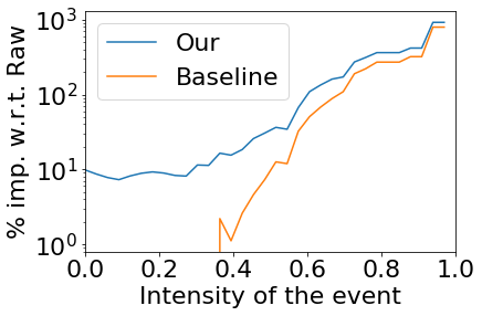
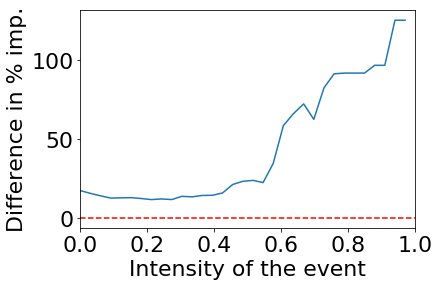
While small temporal variations are very common, however robotic applications are more concerned about large variations which can lead to failure even when they are rare. The goal of photometric calibration is to reduce these large variations in the data such that down-stream applications are less prone to failure. We perform a worst-case analysis on feature-tracking for each dataset. Let us define a worst-event as the occurrence of a large temporal variation similar to the worst temporal variation observed in the dataset. Table II presents the average number of features that were successfully tracked during such worst-events. The more the features, the less prone is the down-stream application to failure. We observe significant improvement of the proposed method over both the baseline and raw datasets. For the “MAV_*” datasets, we observe a negative improvement for the baseline method. To understand the reason, recall that the “MAV_*” datasets contain large spatial variations. The baseline method is developed for RGB cameras and thus assumes a radial model for spatial variations which is not suitable for TIR cameras. This, modelling error leads to worse than uncalibrated performance in these datasets. Next in Figure 4, we also present performance for all magnitude of events (averaged over all the datasets) and not only the worst events. The magnitudes measure the amount of temporal variation and are presented here after normalization with that of the worst event.

Finally, for semi-direct methods, we use the front-end of the popular visual odometry algorithm SVO2.0 [31]. Note that, SVO2.0 does account for illumination gain and offset: parameters related to temporal variation, yet we still observe significant improvement of performance after the proposed calibration (Table I). The performance of baseline can similarly be explained as that of direct method.

IV-B Benefit to Visual Odometry

We evaluate the benefits of photometric calibration towards monocular VO algorithms, using SVO2.0 [31] as a representative. SVO2.0 failed to run reliably on these challenging datasets without calibration, thus, in this context we study and advocate robustness as the primary metric for evaluation rather than VO localization accuracy.

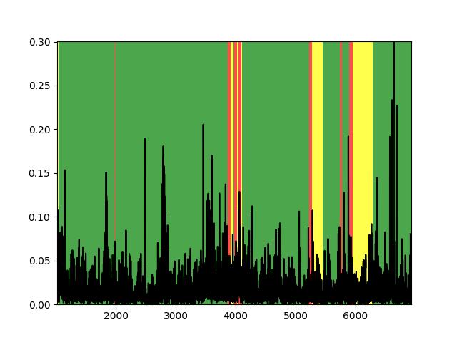
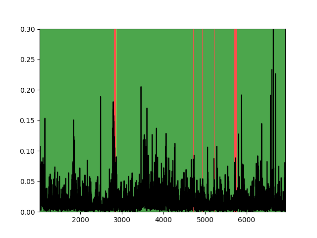
Table III presents the improvement in robustness achieved as measured by two metrics: 1) The percentage of frames that are in “Bad Tracking”, an 2) The number of times SVO2.0 failed completely and had to be restarted in the dataset. We define “Bad Tracking” as the status when SVO2.0 is less confident about the localization estimate. SVO2.0 publishes a “Critical” state message every time that happens (Figure 5). Note that SVO2.0 is a complete VO pipeline with its own robustness measures that include semi-direct feature tracking, keyframe based recovery, feature outlier rejection based on geometric constraints etc., yet we still observe high discrepancy in performance between “Raw” and “Our” versions. The proposed method clearly improves robustness significantly as there are fewer failures. We still observe some failures which might be due to general failure of SVO2.0 due to motion blur and low contrast of TIR images. However, surprisingly we observe high failure rate and “Bad Tracking” for the baseline method. This can again be contributed to the aggressive dift-correction, reduction of contrast and failure to model the spatial variation of TIR camera using a radial model as described in IV-A.

TABLE III: Improvement in Robustness of SVO2.0

Dataset	Percentage of frames			Num Failures
	in Bad Tracking
	Raw	Baseline	Our	Raw	Baseline	Our
AM02	5.43	9.33	2.40	5	9	2
AM05	1.46	9.93	1.46	1	6	1
AM09	3.16	5.75	0.0	2	4	0
MAV_A	0	12.32	0	0	1	0
MAV_B	0	4.72	0	0	1	0

TABLE IV: Mean % of Photometric Error per pixel used to estimate $\mathcal{P}_{s}$ (Training) and the rest of the dataset (Validation)

Dataset	Training Data			Validation Data
	w/o	with	with	w/o	with	with
	Calib	$P^{\prime}_{t}$	$P^{\prime}_{t}$ & $\mathcal{P}_{s}$	Calib	$P^{\prime}_{t}$	$P^{\prime}_{t}$ & $\mathcal{P}_{s}$
AM02	4.88	1.06	1.24	5.20	1.30	1.50
AM05	4.06	1.11	1.97	4.18	0.76	1.10
AM09	4.30	0.89	1.30	4.42	0.84	1.40
MAV_A	4.33	2.36	2.29	3.86	1.92	1.88
MAV_B	3.07	2.12	1.88	2.82	2.48	2.24
MAV_C	2.74	2.56	2.32	3.23	2.69	2.22

TABLE V: Effect of Calibration with and without Drift adjustment. A higher coefficient means that the improvement is more evident for frames with higher photometric error.

Dataset	$\xi_{\text{base}}=0$		$\xi_{\text{base}}=0.025$
	$\rho$	$\rho_{l}$, $\rho_{u}$	$\rho$	$\rho_{l}$, $\rho_{u}$
AM02	0.14	0.03, 0.29	0.52	0.42, 0.62
AM05	0.33	0.15, 0.50	0.42	0.27, 0.55
AM09	0.56	0.47, 0.64	0.50	0.39, 0.59
MAV_A	-0.01	-0.29, 0.27	0.39	0.10, 0.62

Figure 5: SVO2.0 Status over time. Black: measure of photometric error in each frame, Green: Good Tracking, Red: Bad Tracking, Yellow: Trying to initialize. Left: Uncalibrated. Right: Calibrated

IV-C Ablation Study

IV-C1 Generalization of Spatial Parameters

We verify that the the GP Regression model do not overfit and generalize well. To this end, we estimate the average percentage of photometric error per pixel: first without any calibration (w/o Calib), then after applying only temporal calibration (with $P^{\prime}_{t}$) and finally after applying both temporal and spatial calibration (with $P^{\prime}_{t}$ & $\mathcal{P}_{s}$). Training Data refers to $\bar{\mathcal{P}}_{s}$, while Validation Data refers to the set $\mathcal{P}_{s}\setminus\bar{\mathcal{P}}_{s}$ as defined in III-D. As expected in Table IV, we observe that applying $\mathcal{P}_{s}$ reduces photometric error in MAV_* dataset which exhibits significant spatial variations. And we observe that the photometric errors for Training and Validation Data are similar which indicates that the estimates do generalize well. This enables the method to compute $\bar{\mathcal{P}}_{s}\subset\mathcal{P}_{s}$ from sparse correspondences and trust the GP to predict the rest.

IV-C2 With and Without Drift Adjustment

Here we evaluate the contribution of Drift Adjustment and specifically letting $\xi_{\text{base}}>0$. As described in III-C, drift adjustment contains two components. One which attempts to maintain gap between the $c_{t}$ and $b_{t}$ parameters such that they do not collapse and to maintain contrast. And the other component attempts to pull them near their nominal values $c_{t}=1,b_{t}=0$. The former is crucial, and thus always required. However, we may ignore the latter and let the cyclic colormap handle the drift. This is applicable to scenarios when we do not want to introduce a bias on the parameters. However, it does affect low-level performance. Table V presents the pearson correlation coefficient that relates 1) improvement in feature count between calibrated and uncalibrated data, and 2) magnitute of photometric error. The pearson coefficient $\rho$ is accompanied by its $95\%$ confidence interval $[\rho_{l},\rho_{u}]$.

IV-C3 Qualitative Analysis and Computation Time

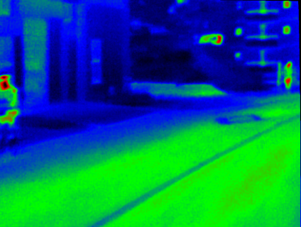
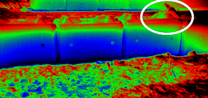
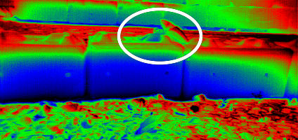
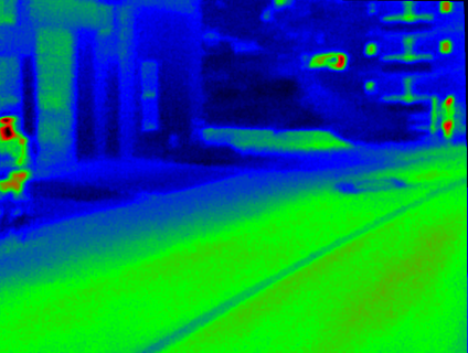
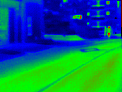
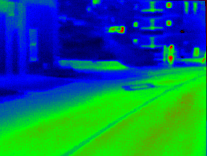
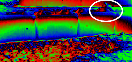
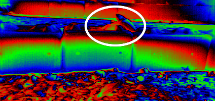
For mapping, it is important that representation of a stationary 3D object as seen in some frame should not change in another frame. Figure 1 and Figure 6 shows the qualitative results over few frames, and we observe that the consistency in representation would improve vision pipelines such as mapping. The average computation time on an Intel Core i7-4710HQ CPU @ 2.50GHz is 0.01 second to estimate $P^{\prime}_{t}$ per frame and 0.027 seconds to estimate $\mathcal{P}_{s}$ per iteration.

(a)

(b)

(c)

(d)

(e)

()

(a)

(b)

(c)

(d)

Figure 6: Top: Uncalibrated. Bottom: Calibrated. First three images show qualitative results on temporal calibration, while the last two shows spatial calibration. Notice how the appearance of an object (marked with white ellipse) changes when viewed at the top right corner of the image as compared to top center position. The camera towards the top corners appear to have accumulated spatial variations.

V Conclusion

In this paper we present a novel system for providing real-time online photometric calibration of thermal infrared cameras. Specifically, we model the sensor acquisition process, investigate the source of photometric error in such cameras and develop an efficient multi-threaded algorithm that can solve for the calibration parameters online. We study the benefits of our proposed method for both low- and high-level vision tasks, and demonstrate qualitative and quantitative improvements in performance over using uncalibrated thermal infrared images sequences. Finally, with this work we hope to take a step towards enabling widespread usage of vision-based methods for thermal-infrared cameras.

VI Acknowledgments

The research described in this paper was carried out at the Jet Propulsion Laboratory, Caltech, under a contract with the National Aeronautics and Space Administration.

References

- [1] C. Brunner and T. Peynot, “Perception quality evaluation with visual and infrared cameras in challenging environmental conditions,” in Experimental robotics. Springer, 2014, pp. 711–725.
- [2] K. Beier and H. Gemperlein, “Simulation of infrared detection range at fog conditions for enhanced vision systems in civil aviation,” Aerospace science and technology, vol. 8, no. 1, pp. 63–71, 2004.
- [3] Y. J. Jeong, S. G. Kang, M. H. Kwon, and H. Jung, “Development of titanium oxide based 12m pixel pitch uncooled infrared detector,” in Infrared Technology and Applications XLIV, vol. 10624. International Society for Optics and Photonics, 2018, p. 106241F.
- [4] E. Terry, X. Lei, B. Morrell, S. Daftry, and A.-A. Agha-mohammadi, “Object and gas source detection with robotic platforms in perceptually-degraded environments.”
- [5] J. Han and B. Bhanu, “Human activity recognition in thermal infrared imagery,” in 2005 IEEE Computer Society Conference on Computer Vision and Pattern Recognition (CVPR’05)-Workshops. IEEE, 2005, pp. 17–17.
- [6] W. Treible, P. Saponaro, S. Sorensen, A. Kolagunda, M. O’Neal, B. Phelan, K. Sherbondy, and C. Kambhamettu, “Cats: A color and thermal stereo benchmark,” in Proceedings of the IEEE Conference on Computer Vision and Pattern Recognition, 2017, pp. 2961–2969.
- [7] T. Mouats, N. Aouf, L. Chermak, and M. A. Richardson, “Thermal stereo odometry for uavs,” IEEE Sensors Journal, vol. 15, no. 11, pp. 6335–6347, 2015.
- [8] P. V. K. Borges and S. Vidas, “Practical infrared visual odometry,” IEEE Transactions on Intelligent Transportation Systems, vol. 17, no. 8, pp. 2205–2213, 2016.
- [9] Y.-S. Shin and A. Kim, “Sparse depth enhanced direct thermal-infrared slam beyond the visible spectrum,” IEEE Robotics and Automation Letters, vol. 4, no. 3, pp. 2918–2925, 2019.
- [10] S. Vidas and S. Sridharan, “Hand-held monocular slam in thermal-infrared,” in 2012 12th International Conference on Control Automation Robotics & Vision (ICARCV). IEEE, 2012, pp. 859–864.
- [11] S. Daftry, M. Das, J. Delaune, C. Sorice, R. Hewitt, S. Reddy, D. Lytle, E. Gu, and L. Matthies, “Robust vision-based autonomous navigation, mapping and landing for mavs at night,” in International Symposium on Experimental Robotics, 2018.
- [12] R. Gade and T. B. Moeslund, “Thermal cameras and applications: a survey,” Machine vision and applications, vol. 25, no. 1, pp. 245–262, 2014.
- [13] Y. K. Choi, N. I. Kim, K. B. Park, S. M. Hwang, J. S. Yoon, and I. S. Kweon, “All-day visual place recognition: Benchmark dataset and baselines,” in CVPR2015 IEEE Conference on Computer Vision and Pattern Recognition. IEEE Computer Society and the Computer Vision Foundation (CVF), 2015.
- [14] S. Khattak, C. Papachristos, and K. Alexis, “Keyframe-based thermal–inertial odometry,” Journal of Field Robotics, 2019.
- [15] C. Papachristos, F. Mascarich, and K. Alexis, “Thermal-inertial localization for autonomous navigation of aerial robots through obscurants,” in 2018 International Conference on Unmanned Aircraft Systems (ICUAS). IEEE, 2018, pp. 394–399.
- [16] H. Budzier and G. Gerlach, “Calibration of uncooled thermal infrared cameras,” Journal of Sensors and Sensor Systems, vol. 4, no. 1, pp. 187–197, 2015.
- [17] L. Chen, L. Sun, T. Yang, L. Fan, K. Huang, and Z. Xuanyuan, “Rgb-t slam: A flexible slam framework by combining appearance and thermal information,” in 2017 IEEE International Conference on Robotics and Automation (ICRA). IEEE, 2017, pp. 5682–5687.
- [18] P. Bergmann, R. Wang, and D. Cremers, “Online photometric calibration of auto exposure video for realtime visual odometry and slam,” IEEE Robotics and Automation Letters, vol. 3, no. 2, pp. 627–634, 2018.
- [19] D. B. Goldman, “Vignette and exposure calibration and compensation,” IEEE transactions on pattern analysis and machine intelligence, vol. 32, no. 12, pp. 2276–2288, 2010.
- [20] S. J. Kim, D. Gallup, J.-M. Frahm, and M. Pollefeys, “Joint radiometric calibration and feature tracking system with an application to stereo,” Computer Vision and Image Understanding, vol. 114, no. 5, pp. 574–582, 2010.
- [21] M. Vollmer and K.-P. Möllmann, Infrared thermal imaging: fundamentals, research and applications. John Wiley & Sons, 2017.
- [22] T. Orżanowski, “Nonuniformity correction algorithm with efficient pixel offset estimation for infrared focal plane arrays,” SpringerPlus, vol. 5, no. 1, p. 1831, 2016.
- [23] G. Bieszczad, T. Orżanowski, T. Sosnowski, and M. Kastek, “Method of detectors offset correction in thermovision camera with uncooled microbolometric focal plane array,” in Electro-Optical and Infrared Systems: Technology and Applications VI, vol. 7481. International Society for Optics and Photonics, 2009, p. 74810O.
- [24] J. Engel, V. Koltun, and D. Cremers, “Direct sparse odometry,” IEEE transactions on pattern analysis and machine intelligence, vol. 40, no. 3, pp. 611–625, 2018.
- [25] M. A. Fischler and R. C. Bolles, “Random sample consensus: a paradigm for model fitting with applications to image analysis and automated cartography,” Communications of the ACM, vol. 24, no. 6, pp. 381–395, 1981.
- [26] S.-X. Li and M. H. Loew, “The quadcode and its arithmetic,” Communications of the ACM, vol. 30, no. 7, pp. 621–626, 1987.
- [27] M. Kuss, “Gaussian process models for robust regression, classification, and reinforcement learning,” Ph.D. dissertation, echnische Universität Darmstadt Darmstadt, Germany, 2006.
- [28] A. Petzoldt, S. Bulygin, and J. Buchmann, “Cyclicrainbow–a multivariate signature scheme with a partially cyclic public key,” in International Conference on Cryptology in India. Springer, 2010, pp. 33–48.
- [29] J. K. Suhr, “Kanade-lucas-tomasi (klt) feature tracker,” Computer Vision (EEE6503), pp. 9–18, 2009.
- [30] P.-E. Sarlin, D. DeTone, T. Malisiewicz, and A. Rabinovich, “Superglue: Learning feature matching with graph neural networks,” in Proceedings of the IEEE/CVF Conference on Computer Vision and Pattern Recognition, 2020, pp. 4938–4947.
- [31] C. Forster, Z. Zhang, M. Gassner, M. Werlberger, and D. Scaramuzza, “Svo: Semidirect visual odometry for monocular and multicamera systems,” IEEE Transactions on Robotics, vol. 33, no. 2, pp. 249–265, 2016.
- [32] T. Qin, P. Li, and S. Shen, “Vins-mono: A robust and versatile monocular visual-inertial state estimator,” IEEE Transactions on Robotics, vol. 34, no. 4, pp. 1004–1020, 2018.
- [33] A. I. Mourikis and S. I. Roumeliotis, “A multi-state constraint kalman filter for vision-aided inertial navigation,” in Proceedings 2007 IEEE International Conference on Robotics and Automation. IEEE, 2007, pp. 3565–3572.
- [34] S. Khattak, C. Papachristos, and K. Alexis, “Keyframe-based direct thermal–inertial odometry,” in 2019 International Conference on Robotics and Automation (ICRA). IEEE, 2019, pp. 3563–3569.