Powder vibration studied by Mössbauer spectroscopy

Abstract

Mössbauer spectroscopy is applied to study ultrasound vibration of a granular material. A pile of powder is placed onto the surface of piezo transducer vibrated with the frequency 12.68 MHz. The size of grains (1.3 $\mu$m) is much smaller than the wavelength of ultrasound, but much larger than the vibration amplitude. Due to vibration a single line of the Mössbauer transmission spectrum is split into a comb structure with a period equal to the vibration frequency. This spectrum contains the information about fast and slow modes in granular dynamics. We developed a method which allows to measure decay of ultrasound in the granular material and to estimate the results of the particle convection of grains in the pile.

I Introduction

A granular material is conventionally considered as a conglomeration of discrete macroscopic objects, which are larger than that composing mesoscopic or microscopic media. The size of particles making up a granular medium is large enough such that they are not subject to thermal Brownian motion. Therefore, the lower limit of particle diameter is about 1 $\mu$m Duran . Collective behavior of a granular medium is characterized by a loss of energy, for example, due to friction when particles collide. However, despite its simplicity such a system behaves differently from any of the other familiar forms of matter - solids, liquids, or gases. If granular materials are excited, for example, vibrated or allowed to flow, grains exhibit a wide range of pattern forming not a single phase of matter but have characteristics reminiscent of solids, liquids, or gases Jaeger . The famous Brazil nuts effect, demonstrating that the larger or lighter grains are always found on top of the shaken box of multigrain müesli, is explained via a model that includes sequential as well as nonsequential (cooperative) particle dynamics Ristow . Avalanche of particles, bulk convection of grains to the top of the pile, phase transition are phenomena that demonstrate exceptional properties of granular materials Ristow ; Eshuis ; Herrmann ; Klongboonjit ; Liu ; Nagel . They play an important role in industries, such as mining, agriculture, construction, pharmaceutics, etc. The extraction of ores, sands, and gravel, which relies on dredging, crushing and grinding, followed by separation, are commonly used for production of granular materials. Therefore, improvement and optimization in methods of transport, storage and mixing would have a major economic impact. The cosmetic and pharmaceutical industries, specialized chemistry, and the food industry demand increasingly sophisticated processing technologies when it is absolutely essential to achieve intimate mixing of different granular materials without their separation. Ultrasonic microfeeding of fine powders is a promising method for solid freeform fabrication by 2D and 3D printing and pharmaceutical dosing Lu .

Recent scientific progress in knowledge about open nonequilibrium systems and development of modern computational methods give impetus to studying of granular dynamics Ristow . Granular material is a multiparticle system. Therefore, many mathematical models are simplified to one-dimensional or two-dimensional examples. Interparticle forces in granular materials such as the static friction at particle contacts, their collision, and particle-wall contacts are well studied for two-dimensional systems Majmudar . Analysis of real-life three-dimensional situations is still quite complicated. However, with some assumptions and simplifications the problem can be solved for model systems Bougie ; Harada ; Amirifar .

Experimentally, the low frequency vibration of granular material was studied by optical methods in two-dimensional system (8 to 30 Hz vibration) Clement , by means of nuclear magnetic resonance (NMR) of poppy seeds in three-dimensional system subject to the periodic sequence of shakes (each shake consists of a single 20-Hz sinusoidal period of acceleration separated by 0.7 s between shakes) Nagel2 . Measurements in three-dimensional medium, vibrated with frequency 30-100 Hz, was also performed by observation of a thin radioactive-marker layer sandwiched between studied granular layers Harwood . In this experiment migration of marker could be followed in either an upward or downward direction.

High frequency vibration over frequency range from 100 to 350 kHz is used in experiments studying marine sediments, which are composed of unconsolidated granular materials Buck . Gaussian burst signals with center frequencies 0.4 - 1.6 MHz where used to excite ultrasound pulses in granular media by piezoelectric transducer Zhai . Piezoelectric transducer also were employed in this experiment to detect longitudinal sound waves and X-ray diffraction provided tomography of contact fabric, particle kinematics, average per-particle stress tensors, and interparticle forces.

Ultrasound vibration of granular medium induces slow and fast modes in granular dynamics. Time scales of these modes are well separated Mehta . Transport of grains producing bulk convection, size segregation, and dynamical phase transition are relatively slow. They can be studied by optical methods, X-ray diffraction, or NMR tomography. Fast modes are difficult to trace. Only attenuation of the longitudinal sound wave can be detected at the exit of the granular medium excited from the opposite side Zhai .

It is interesting to note that, for example, a column of beads or other elastic granular material vibrated vertically demonstrate distinct behavior depending on the acceleration $A_{\text{acs}}=a\Omega^{2}$ given by the vibrated plate at the bottom of the column, where $a$ and $\Omega$ are the amplitude and frequency of the plate vibration. When acceleration is small, the system is in a ”condensed” state where the beads are practically in contact with each other moving in unison. When acceleration is large, the system is in a ”fluidized” state, with the beads moving individually much like particles in a gas or a fluid Duran . In this state the kinetic energy $E_{\text{kin}}=ma^{2}\Omega^{2}/2$ is the main parameter defining the system dynamics. Transition between two states is defined by a parameter $\Lambda=A_{\text{acs}}/g$, where $g$ is gravitational acceleration. Usually, when $\Lambda>1$ the qualitative behavior of particles changes. However, this condition depends on individual particle mass and friction force Duran .

In this paper we study ultrasonic vibration of powder consisting of grains of potassium ferrocyanide K₄Fe(CN)${}_{6}\cdot$3H₂O. It is the potassium salt, which forms monoclinic crystal. The salt is grind up to produce crystallites with sizes satisfying the lognormal distribution with a median size of 1.3 $\mu$m and a standard deviation of 0.18. This powder is vibrated by polymer (PVDF) piezoelectic transducer with frequency 12.68 MHz. The wavelength of the ultrasound generated in the solid grains is several hundred microns, i.e., much larger than the size of an individual particle. The amplitude $a$ of ultrasound vibration, induced by piezoelectic transducers, is usually extremely small. Our previous experiments showed that thin PVDF transducer is capable producing 25 $\mu$m thick stainless-steel foil vibration with frequency 12.68 MHz and amplitude $a$ about one angstrom Shakhmuratov1 ; Shakhmuratov2 . Rough estimation of the acceleration $A_{\text{acs}}$ imparted to the objects placed on the surface of the transducer gives the value $5.4\times 10^{5}$ m/s², which is comparable with a bullet’s acceleration in the barrel of a pistol. Therefore the parameter $\Lambda$ is extremely large.

Vibration of the salt grains, enriched by ⁵⁷Fe isotope, is studied by Mössbauer spectroscopy where 14.4-keV $\gamma$-radiation is used to observe the absorption spectrum of ⁵⁷Fe nuclei. This method has many advantages since the wavelength of such a radiation is slightly below one angstrom (86 pm) and quality factor $Q$ of the ⁵⁷Fe absorption line is extremely large, i.e., $Q=\omega_{A}/\Gamma_{A}=3\times 10^{12}$, where $\omega_{A}$ is the resonant frequency and $\Gamma_{A}$ is the width of the absorption line.

When the quasi-monochromatic source radiation with main frequency $\omega_{S}$ is transmitted through a medium with resonant nuclei, which are vibrated, the spectrum of the radiation field is transformed into polychromatic with a set of spectral lines $\omega_{S}\pm n\Omega$, where $\Omega$ is the vibration frequency and $n=0,\pm 1,\pm 2$ Shakhmuratov1 ; Shakhmuratov2 ; Cranshaw ; Mishroy ; Asher ; Tsankov ; Shvydko ; Shakhmuratov3 . These lines are produced by Raman scattering, which is inelastic scattering of $\gamma$-radiation by vibrating nuclei. The intensities of the spectral components and their dependence on the vibration amplitude give the information about the decay of ultrasound and the distribution of the vibration amplitudes along the medium. Thus, our experiments are capable to provide the information about fast mode in granular dynamics (ultrasound vibration and decay along the granular medium) and verify the models of slow mode including slow flow and convection.

II Method

In Mössbauer spectroscopy a radiation source and absorber are basic elements. For example, for the solid absorber containing ⁵⁷Fe nuclei the solid source matrix with inclusions of radioactive nuclei ⁵⁷Co is usually used. These nuclei decay randomly emitting $\gamma$-photons with the energy 14.4 keV and spectral width $\Gamma_{S}$. For a single line source the minimum value of this width is $\Gamma_{0}=1.1$ MHz. Activity of the commercially available sources allows to produce a random flow of single $\gamma$-photons with the average rate about $10^{4}$ photons per second. Slow motion of the radiation source with respect to the absorber gives the oppotunity to scan the absorption line of ⁵⁷Fe due to Doppler effect. To accumulate absorption spectrum, the electric pulses produced by $\gamma$-detection system must be recorded synchronously to the sweep velocity of the source. Collecting number of counts corresponding to different velocities within fixed time windows, we obtain absorption spectrum, which is seen as a drop of counts at resonance and constant rate of counts far from resonance. Since the coherence length of $\gamma$-photons is 141 ns, which is the duration of a single-photon pulse, we have a snapshot of fast processes, for example, vibration of nuclei with frequency larger than $\Gamma_{S}$. Typical data-acquisition time for one Mössbauer spectrum may range from several hours to several days, depending on resonant nuclei concentration and absorber thickness. Therefore, these spectra contain information about slow steady-state processes averaged over a long time period and reflecting slow dynamics of grains with ⁵⁷Fe nuclei such as slow flow and convection.

The Fourier transform of the radiation field amplitude emitted by the source nucleus is

$$E_{S}(\omega)=\frac{E_{0}e^{ikz}}{\Gamma_{S}/2+i(\omega_{S}-\omega)}.$$ (1)

where $E_{0}$ and $k$ are the amplitude and wave number of the radiation field emitted by the source nucleus, respectively (see Appendix A).

Transmission probability of a single $\gamma$-photon through the resonant absorber is described by equation (see Ref. Gutlich and Appendix A)

$$N_{\text{out}}(\omega_{A}-\omega_{S})=\frac{\Gamma_{0}}{2\pi}\int_{-\infty}^{\infty}\frac{\exp\left[-\frac{T_{A}(\Gamma_{0}/2)^{2}}{\left(\Gamma_{A}/2\right)^{2}+(\omega_{A}-\omega)^{2}}\right]}{\left(\Gamma_{S}/2\right)^{2}+(\omega_{S}-\omega)^{2}}d\omega,$$ (2)

where $\omega_{A}$ and $\Gamma_{A}$ are the frequency and linewidth of the absorber nuclei, $T_{A}=f_{A}n_{A}\sigma_{A}$ is the effective (optical) thickness of the absorber, $f_{A}$ is the Debye-Waller factor for nuclei in the solid state absorber denoting the fraction of $\gamma$-emission or absorption occurring without recoil, $n_{A}$ is the number of ⁵⁷Fe nuclei per unit area of the absorber, and $\sigma_{A}$ is the resonant absorption cross section. Here, for simplicity, nonresonant absorption and the fraction of the radiation field with recoil are disregarded. They can be easily taken into account in experimental data analysis. Example of $N_{\text{out}}(\omega_{A}-\omega_{S})$ function is shown in Fig. 1 by dotted blue line.

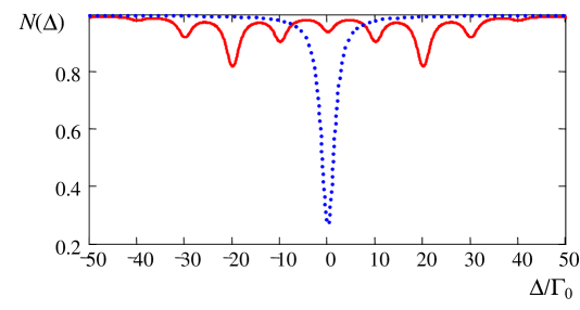
Figure 1: (color on line) Dependence of the detection probability on $\Delta=\omega_{A}-\omega_{S}$. Blue dots correspond to $N_{\text{out}}(\Delta)$, which describes standard Mössbauer spectrum, Eq. (2). Red line shows Mössbauer spectrum, $N_{SV\text{out}}(\Delta)$, for the source vibrated with frequency $\Omega=10\Gamma_{0}$ and modulation index $M=3$, see Eq. (7). Effective thickness of the absorber is $T_{A}=5$

II.1 Vibrating source

To explain the main points of the method used in this paper we will first consider an example when the source nucleus vibrates with the frequency $\Omega$ and the absorber is motionless. Then, the distance between the source and absorber oscillates as $z_{\text{vib}}=z+a\sin(\Omega t+\psi)$, where $a$ and $\psi$ are the amplitude and phase of the vibration. The radiation field of the source is $E_{S}(t-t_{0})=E_{0}\theta(t-t_{0})e^{-(i\omega_{S}+\Gamma_{0}/2)(t-t_{0})+ikz}$, where $t_{0}$ is the instant of time when the excited state nucleus is formed in the source and $\theta(t-t_{0})$ is the Heaviside step-function. Nuclei of the absorber interact with the field whose phase is modulated due to oscillation of the distance $z_{\text{vib}}$. Therefore, the source field modifies as follows

$$E_{SV}(\tau)=E_{S}(\tau)e^{ika\sin[\Omega(\tau+t_{0})+\psi]},$$ (3)

where $\tau=t-t_{0}$. According to the Jacobi-Anger formula this expression can be presented as

$$E_{SV}(\tau)=E_{S}(\tau)\sum_{n=-\infty}^{+\infty}J_{n}(M)e^{in[\Omega(\tau+t_{0})+\psi)]},$$ (4)

where $J_{n}(M)$ is the $n$th order Bessel function, $M=ka=2\pi a/\lambda$ is the modulation index of the field phase, and $\lambda$ is the radiation wavelength. Due to vibration of the source the single line radiation field with frequency $\omega_{S}$ transforms into polychromatic, consisting of a set of spectral lines $\omega_{S}-n\Omega$ with $n=0,\pm 1,\pm 2,...$ Fourier transform of this field is

$$E_{SV}(\omega)=E_{0}\sum_{n=-\infty}^{+\infty}\frac{J_{n}(M)e^{in\phi}}{\Gamma_{0}/2+i(\omega_{S}-n\Omega-\omega)},$$ (5)

where $\phi=\Omega t_{0}+\psi$. Here and below for shortening $ikz$ is omitted in the exponent. After passing through the absorber with a single resonance line this field is transformed as

$$E_{SV\text{out}}(\omega)=E_{0}\sum_{n=-\infty}^{+\infty}\frac{J_{n}(M)e^{-\frac{T_{A}\Gamma_{A}/4}{\Gamma_{A}/2+i(\omega_{A}-\omega)}+in\phi}}{\Gamma_{0}/2+i(\omega_{S}-n\Omega-\omega)}.$$ (6)

Calculating the probability of photon detection at the exit of the absorber in the same way as in the case of the nonvibrating source (see Appendix A), we obtain

$$N_{SV\text{out}}(\Delta)=\sum_{n=-\infty}^{+\infty}J_{n}^{2}(M)L(\Delta_{n}),$$ (7)

where $\Delta=\omega_{A}-\omega_{S}$, $\Delta_{n}=\omega_{A}-\omega_{S}+n\Omega$, and

$$L(\Delta_{n})=\frac{\Gamma_{S}}{2\pi}\int_{-\infty}^{+\infty}\frac{e^{-\frac{T_{A}(\Gamma_{0}/2)^{2}}{(\Gamma_{0}/2)^{2}+(\omega_{A}-\omega)^{2}}}}{(\Gamma_{0}/2)^{2}+(\omega_{S}-n\Omega-\omega)^{2}}d\omega.$$ (8)

This expression is valid if $\Omega\gg\Gamma_{0}$, which means that the distance between the spectral lines of the source is much larger than the linewidth of the absorber. Therefore, the contribution of cross terms, such as $J_{n}(M)J_{m}(M)$, is negligible. Comparison of $N_{\text{out}}(\Delta)$ with $N_{SV\text{out}}(\Delta)$ is shown in Fig. 1.

Far form resonance for all individual spectral components of the source with the single line absorber, i.e., when $\left|\Delta_{n}\right|/\Gamma_{0}\gg 1$, the function $L(\Delta_{n})$ equals unity for all $n$. In this case all the spectral components of the vibrating source pass through the motionless absorber without interaction. Then, due to identity

$$\sum_{n=-\infty}^{+\infty}J_{n}^{2}(M)\equiv 1,$$ (9)

we have $N_{SV\text{out}}(\Delta)=1$.

When, for example, $n$th component comes close to resonance with the absorber ($\omega_{S}-n\Omega\approx\omega_{A}$), then

$$N_{SV\text{out}}(\omega_{A}-\omega_{S})=1-J_{n}^{2}(M)\left[1-L(\Delta_{n})\right],$$ (10)

i.e., only resonant component of the field interacts with the absorber, while other components pass through without interaction. This expression is derived with the help of identity (9). At $\omega_{A}-\omega_{S}=-n\Omega$, the detection probability of a single photon drops down to

$$N_{SV\text{out}}(n\Omega)=1-J_{n}^{2}(M)\left[1-N_{\text{out}}(0)\right].$$ (11)

The scale of the decrease in the photon probability at the exit of the absorber is defined by the square of the corresponding Bessel function, $J_{n}^{2}(M)$.

II.2 Vibrating absorber

If the absorber vibrates with respect to the motionless source, the radiation field $E_{AV}(\tau)$ in the coordinate system rigidly bounded to the absorber sample is again acquires a comb structure with spectral componets $\omega_{S}-n\Omega$ where $n=0,\pm 1,\pm 2,...$, i. e., $E_{AV}(\tau)=E_{SV}(\tau)$, see Eq. (4).

We calculated the field, transmitted through the absorber, and transformed the output field back to the lab frame (see Appendix A). If all spectral components of the comb $E_{AV}(\tau)$ in the vibrating frame are far from resonance with the single line absorber, then their amplitudes do not change. In this case Fourier transform of the output field in the lab frame, $E_{L}(\omega)T,$ does not change also, i.e., $E_{L}(\omega)=E_{S}(\omega)$. Then, the probability of its registration is unity, i.e., equals to $N_{0}=1$.

If $n$th component of the comb is close to resonance with the absorber and other spectral components are far from resonance, then

$$E_{L}(\omega)=E_{S}(\omega)+E_{R}(\omega),$$ (12)

$$E_{R}(\omega)=-E_{0}J_{n}(M)\sum_{m=-\infty}^{+\infty}\frac{J_{m}(M)e^{i(n-m)\phi}\left[1-e^{-\frac{T_{A}\Gamma_{A}/4}{\Gamma_{A}/2+i(\omega_{A}+m\Omega-\omega)}}\right]}{\Gamma_{0}/2+i[\omega_{S}-(n-m)\Omega-\omega]},$$ (13)

where $E_{R}(\omega)$ is the field scattered by the vibrating absorber. The scattered field is polychromatic containing the resonant for the absorber component with frequency $\omega_{S}=\omega_{A}+n\Omega$ and Raman components $\omega_{S}-(n-m)\Omega=\omega_{A}+m\Omega$ with $m\neq n$. The resonantly scattered component is in antiphase with the incident radiation reducing its intensity due to destructive interference. The Raman components appear due to inelastic scattering of the incident radiation field on the vibrating nuclei. The amplitudes of these components depend on $J_{n}(M)$, i.e., on the amplitude of the resonant component in the frequency comb $E_{AV}(\tau)$.

At exact resonance ($\omega_{S}=\omega_{A}+n\Omega$), Eq. (13) can be expressed as

$$E_{R}(\omega)=-E_{0}\left[J_{n}^{2}(M)K_{n}(\omega)+J_{n}(M)\sum_{\begin{subarray}{c}m=-\infty\\ (m\neq n)\end{subarray}}^{+\infty}J_{m}(M)K_{m}(\omega)e^{i(n-m)\phi}\right],$$ (14)

where

$$K_{m}(\omega)=\frac{\left[1-e^{-\frac{T_{A}\Gamma_{A}/4}{\Gamma_{A}/2+i(\omega_{A}+m\Omega-\omega)}}\right]}{\Gamma_{0}/2+i(\omega_{A}+m\Omega-\omega)},$$ (15)

The maxima of the functions $K_{m}(\omega)$, which take place at frequencies $\omega_{m}=\omega_{A}+m\Omega$, are the same for all spectral components $m$, i.e., resonant $n$ and Raman components $m\neq n$. Therefore, the maximum amplitudes of the spectral components are proportional to $J_{n}(M)J_{m}(M)$ with the same factor $K_{m}(\omega_{m})=2\left(1-e^{-T_{A}/2}\right)/\Gamma_{0}$.

In spite of the difference between the output fields for the vibrating source and motionless absorber, Eq. (6), and for the source and vibrating absorber, Eq. (12), the probability of photon detection at the exit of the vibrated absorber is described by the same expression as for the vibrating source, see Eqs. (7) and (10). This is because the transformation back to the lab frame does not influence the time integrated intensity of the radiation field, which coincides in the vibrating frame with the radiation field of the vibrated source transmitted through the motionless absorber.

III The Model

We studied Mössbauer spectra of potassium ferrocyanide powder placed on PVDF piezo transducer. The pile of powder was made thin (about 100 $\mu$m thick) and perfectly flat, as well as possible, by stirring. Vibration of grains with frequency $\Omega=12.68$ MHz splits the single absorption line into a comb structure with a frequency period equal $\Omega$. This splitting appears only after a long time preparation period. We suppose that the preparation period is needed to form densely packed grains corresponding to the solid phase located in the pile bottom on the surface of the transducer. Otherwise, acoustic contact between piezo transducer and powder is not formed and absorption line is not split. We noted that slow convection also took place since small traces of grains were found around the pile after preparation period and experimental data collection. Therefore, we suppose that grains at the top of the pile form a gas-like phase and some of the grains are thrown out from the pile top due to vibration.

Wavelength of ultrasound in potassium ferrocyanide is nearly four times large than the thickness of the powder pile. Therefore, one could expect piston-like vibration of the absorber. Example of the Mössbauer transmission spectrum for the grains vibrated in unison with the same amplitude is shown in Fig. 1. Since the depth of $n$-th component of the spectrum is proportional to the oscillating function $J_{n}^{2}(M)$, the pattern of the comb minima forms a nonmonotonous envelope with oscillations. Similar spectra were observed in experiments Shakhmuratov1 ; Shakhmuratov2 ; Mkrtchyan77 ; Mkrtchyan79 where the vibration of the stainless steel (SS) foil was studied. It is also possible even suppressing almost to nonabsorbing level the central component of Mössbauer spectrum with $n=0$ when modulation index is $M=2.4$ since $J_{0}^{2}(2.4)=0$. This results in acoustically induced transparency of the absorber for $\gamma$-radiation. Experimental implementation of the transparency effect was demonstrated for SS foil in Ref. Radeon .

Meanwhile, our Mössbauer spectra for the vibrated powder demonstrate qualitatively different pattern. Comb minima follow a bell-shape envelope and the central component is always dipper than others for all values of the modulation index, which depends on RF power applied to piezo transducer, see Fig. (2). Similar spectra were observed for powder pressed in a tablet onto the surface of piezo transducer Shakhmuratov1 and powder suspended in viscous liquid or resin Cranshaw ; Shakhmuratov3 . One may assume that grains in a pile or grains in a resin vibrate with the same frequency but their amplitudes are different depending on the distance from the transducer. The phase of vibrations cannot be chaotic and randomly changing in a time scale comparable with the vibration period $2\pi/\Omega$. Otherwise, the components of the comb spectrum will be broadened progressively with increase of the number $n$. This is because of the phase factor $e^{in\psi}$ in the expression for the field $E_{AV}(\tau)=E_{SV}(\tau)$, see Eq. (4). Phase jitter $\psi(t)$, if present, produces broadening of the $n$-th component of the absorption line changing $\Gamma_{0}/2$ to $\Gamma_{0}/2+n^{2}\left\langle(\delta\psi_{t})^{2}\right\rangle/2\tau_{c}$, where $\left\langle(\delta\psi_{t})^{2}\right\rangle$ is the phase variance, $\delta\psi_{t}=\psi(t)-\psi(0)$, and $\tau_{c}$ is a correlation time of the phase change, see, for example, Refs. Shakhmuratov1 ; Shakhmuratov4 . However, no difference in the linewidths of the components of the Mössbauer transmission spectrum are found in the experiments with grains. One can find similar arguments in Ref. Monahan where quantum beats of recoil-free $\gamma$-radiation in time domain experiments are observed and theoretically described. Interference terms $\left\langle J_{n}(M)J_{l-j}(M)\right\rangle$ producing quantum beats are not attenuated according to the law $\exp[-j^{2}\sigma^{2}/2]$, which would be present if $\psi$ is normally distributed about $\psi=0$ with variance $\sigma^{2}$.

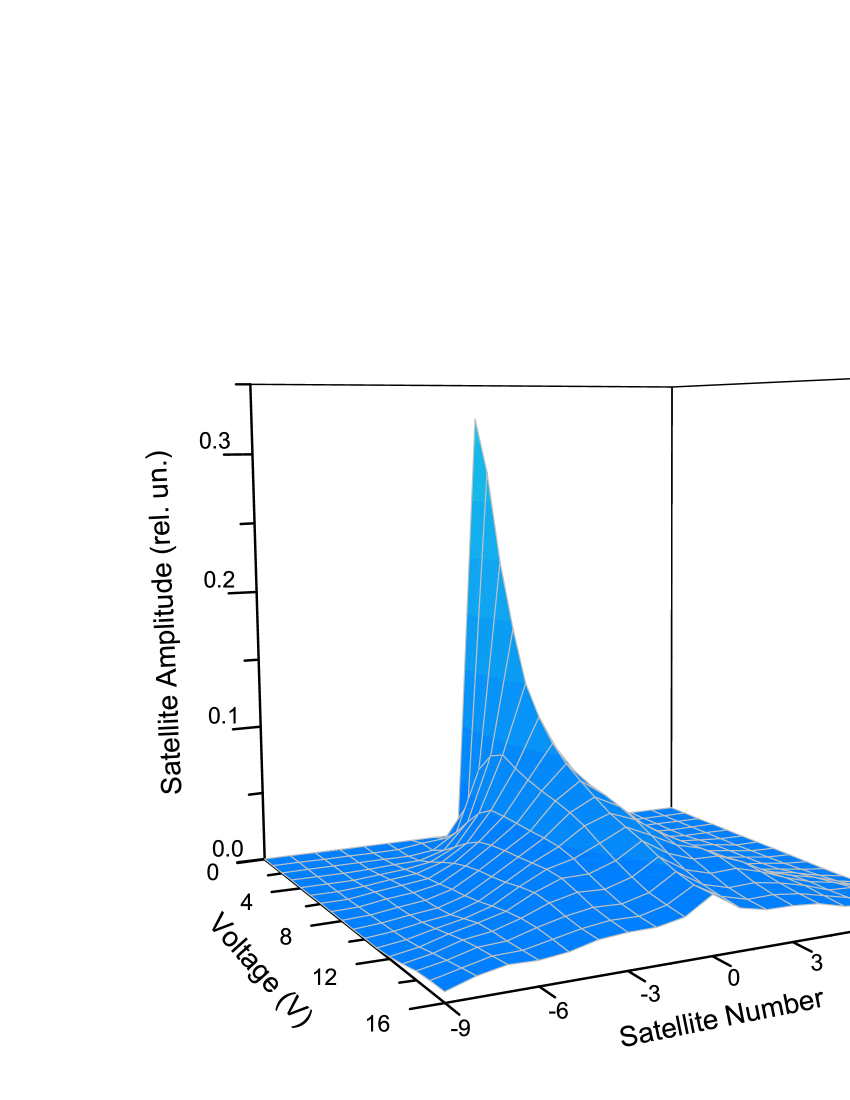
Figure 2: (color on line) Experimentally observed dependence of the absolute values of the transmission dips, presented as the envelope line connecting the dips of the spectral components, reverted upside down. Examples of the transmission spectra are shown in Fig. 3. Front axis (x) shows the number of the spectral component, vertical axis (z) is the absolute value of the depth of the spectral component, which is $1-N_{SV\text{out}}(\omega_{A}-\omega_{S})$, and y axis on the left is the voltage of the RF generator applied to the piezo transducer.

We model vibration of the powder pile by oscillating granular layers. A flat layer of grains in the pile bottom is pushed up by the piezo transducer. Next layer of grains is excited by the first layer, etc. We assume that vibration amplitudes of the layers decrease from the pile bottom to the top. The granular bed behaves much like a solid comoving with the vibrating piezo transducer. However, because $\Lambda\gg 1$ some grains may detach from the transducer resulting in the particle convection. They move upward at the pile center and downward at the edges. Vibration of grains can be decomposed into coherent and incoherent parts. The coherent portion is dominant representing the average of many measurements, while the incoherent portion gives less contribution to Mössbauer spectrum that diminishes when averaged in repeated measurements Zhai . This is because time scales of slow and fast modes in grain dynamics are well separated. We also take into account grain convection introducing the averaging over the angle between vertical axis and direction along which an individual grain vibrates.

We model the Mössbauer transmission spectrum by the expression

$$N_{\text{out}}(\omega_{A}-\omega_{S})=e^{-\mu D}\left[(1-f_{S})+f_{S}\mathcal{L}(\omega_{A}-\omega_{S})\right],$$ (16)

where $\mu$ is nonresonant absorption coefficient, $D$ is the thickness of the pile of powder, $f_{S}$ is the recoil-free fraction of $\gamma$-emission of the source, and the function $\mathcal{L}(\omega_{A}-\omega_{S})$ is

$$\mathcal{L}(\omega_{A}-\omega_{S})=1-\sum_{n=-\infty}^{+\infty}C_{n}\mathcal{L}_{n}(\omega_{A}+n\Omega-\omega_{S}).$$ (17)

To simplify experimental data analysis, the function $\mathcal{L}_{n}(\omega_{A}+n\Omega-\omega_{S})$ is approximated by Lorentzian

$$\mathcal{L}_{n}(\omega_{A}-\omega_{S})=\frac{B_{\exp}\Gamma_{\exp}^{2}}{(\omega_{A}+n\Omega-\omega_{S})^{2}+\Gamma_{\exp}^{2}},$$ (18)

where $B_{\exp}$ together with $C_{n}$ define the maximum depth of the $n$-th spectral component of the Mössbauer transmission spectrum and $\Gamma_{\exp}$ is the width of this component, which is taken the same for all components. Parameters $B_{\exp}$ and $\Gamma_{\exp}$ are found from fitting to the experimental spectra.

We assume that the vibration amplitude of the grains in the pile decays as $a(x)=a_{0}\exp(-\gamma x)$, where $a_{0}$ is the amplitude at the pile bottom, $x$ is the distance from the bottom to a particular upper layer of grains, and $\gamma$ is a decay constant. Then, the coefficients $C_{n}$ can be calculated according to Eq. (71), where $M(x)=M_{0}\exp(-\gamma x)$ and $M_{0}$ is the modulation index at the pile bottom, see Appendix B.

In our model we assume that slow mode of granular dynamics producing particle convection builds up chains of the strongly contacting grains, which form the fastest ultrasound wave paths, see Ref. Zhai . These paths are tortuous slowly fluctuating in time. To take this slow process into account in the fast mode of granular dynamics we introduce averaging over the angle $\alpha$ between the vertical axis and direction along which an individual particle vibrates in the chain. Then, the coefficients $C_{n}$ in Eq. (17) can be expressed as follows

$$C_{n}=\frac{1}{D}\int_{0}^{D}dx\int_{0}^{\pi/2}d\alpha\frac{e^{-\alpha^{2}/2\alpha_{m}^{2}}}{U(\alpha_{m})}J_{n}^{2}[M(x)\cos\alpha],$$ (19)

where

$$U(\alpha_{m})=\alpha_{m}\sqrt{\frac{\pi}{2}}\operatorname{erf}\left(\frac{\pi/2}{\sqrt{2}\alpha_{m}}\right),$$ (20)

and $\alpha_{m}^{2}$ is the variance of the angle distribution. It is also possible introducing the dependence of $\alpha_{m}$ on distance $x$. However, this modification complicates experimental data analysis and we decided to take $\alpha_{m}$ as a constant parameter.

IV Experimental results

A conventional Mössbauer spectrometer is used in experiment. The source, ⁵⁷Co:Rh, is mounted on the holder of the Mössbauer drive Doppler shifting the frequency of the radiation of the decaying nuclei. The absorber was made of K₄Fe(CN)${}_{6}\cdot 3$H₂O powder with effective thickness $T_{A}=13.2$. Actually, the absorber was a homogeneous mixture of powder with natural abundance of ⁵⁷Fe ($\sim 2\%$) and enriched one (95$\%$). The enriched powder was produced by M. N. Mikheev Institute of Metal Physics, Ural Branch of Russian Academy of Sciences, Yekaterinburg. Average abundance of ⁵⁷Fe in powder mixture was nearly $50\%$. Physical thickness of the absorber, $D$, was close to 100 $\mu$m. The preparation of the absorber is described at the end of the Introduction in Sec. I . The source was placed below the absorber and the detector was mounted above the absorber. This vertical geometry of the experiment allowed to keep a powder on the surface of the vibrating transducer due to gravity. As a transducer we used a polyvinylidene fluoride (PVDF) piezo polymer film (thickness 28 $\mu$m, model LDT0-28K, Measurement Specialties, Inc.). A piece of 10$\times$12 mm polar PVDF film was coupled to a plexiglas backing of $\sim$2 mm thickness with epoxy glue. The PVDF film transforms the sinusoidal signal from the radio-frequency (RF) generator into a uniform vibration of the absorber nuclei in the bottom of the powder pile, which is in a mechanical contact with the PVDF film.

Examples of the experimentally observed spectra are shown in Fig. 3. They are fitted by the theoretical model, Eq. (16). Three main fitting parameters of the model are the modulation index $M_{0}$, the decay of the vibration amplitude in the vertical direction, $\gamma$, and the standard deviation, $\alpha_{m}$, of the particle vibration angle from vertical direction. Optimal value of the first parameter for all voltages (the global parameter) is $\gamma D=1.38\pm 0.04$. Thus, the value of the vibration decay constant is $\gamma=1.38\times 10^{-4}$m^-1. The dependencies of the parameters $M_{0}$ and $\alpha_{m}$ on the RF voltage V are shown in Fig. 4.

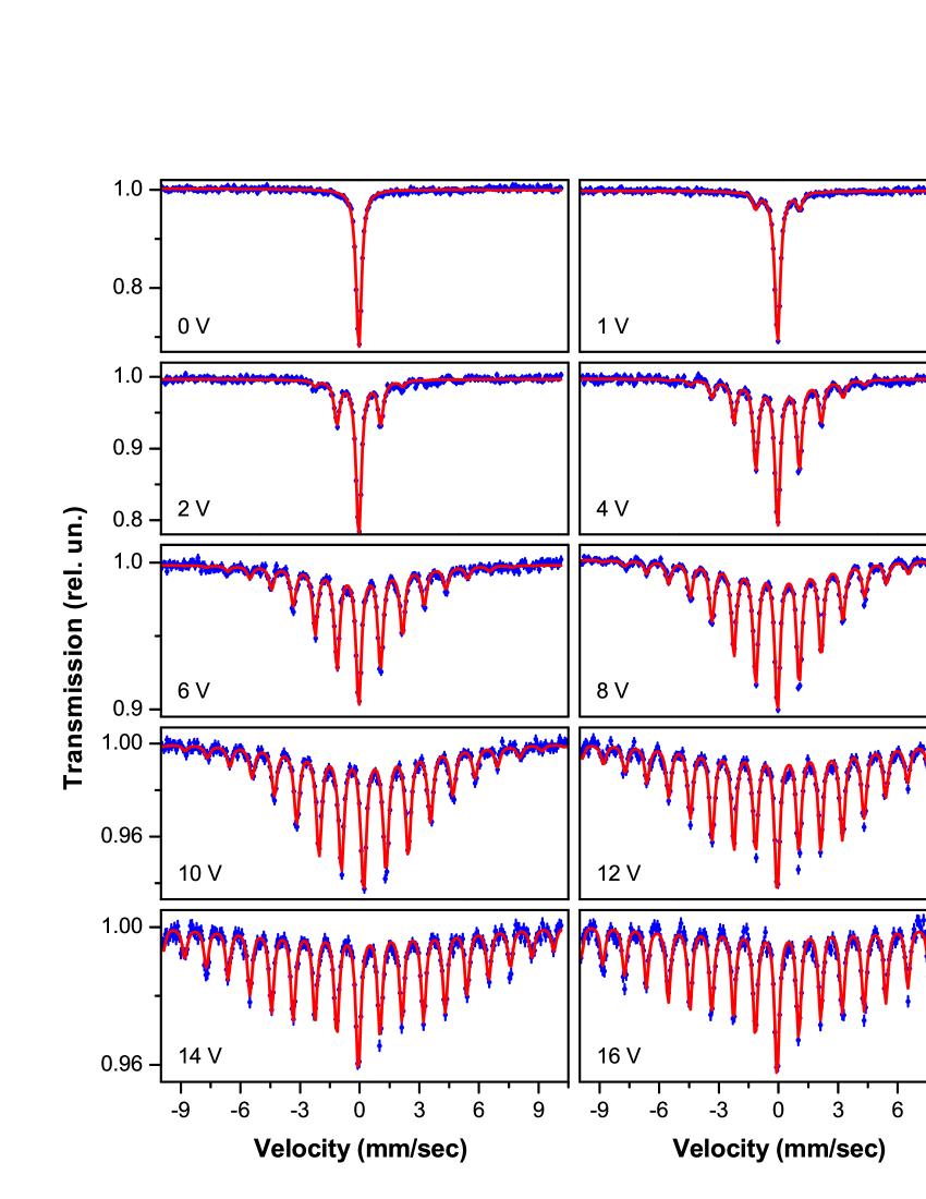
Figure 3: (color on line) The Mössbauer transmission spectra for the vibrated powder. Horizontal axis is the source velocity (in mm/sec) Doppler shifting the frequency of the source. Vertical axis is the transmission probability, normalized to unity far from resonance. The value of the RF voltage applied to the piezo transducer is shown in the bottom of the left corner in each panel. Blue dots are experimental data and red line is the theoretical fitting.

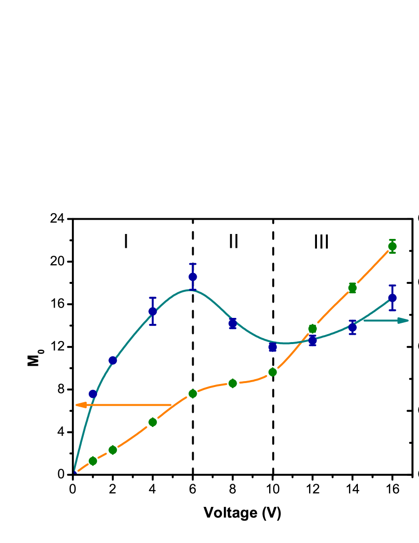
Figure 4: (color on line) Dependences of the modulation index $M_{0}$ for the powder bed (orange line) and standard deviation of the vibration angle, $\alpha_{m}$, (dark cyan line) on the RF voltage, V, applied to the piezo transducer. In both plots dots correspond to the parameters derived from fitting and the lines connecting the dots are shown for visualization. For some dots error bar coincides or smaller than the size of the dot.

Modulation index $M_{0}$, shown by orange line, monotonously rises with the RF voltage increase. In the plot for $M_{0}$ versus V, there are three domains with different slopes separated by vertical dashed lines. In the first domain (I) standard deviation $\alpha_{m}$ of the angle $\alpha$, shown by dark cyan line, gradually rises with the voltage increase reaching the value close to $\alpha_{m}=\pi/2$. This means that at the right border of the first domain appreciable fraction of grains vibrate in horizontal direction or do not vibrate at all since the modulation index in Eq. (19) is $M(x)\cos\alpha$. We may assume that when RF voltage is 6V many chains of the strongly contacting grains become very tortuous or even broken. For this voltage the parameter $M_{0}$ is 7, which gives vibration amplitude of the bed grains $a=95.8$ pm.

As was mentioned in the Introduction, the kinetic energy of the vibrated grain, $E_{\text{kin}}=ma^{2}\Omega^{2}/2$, plays an important role in granular dynamics. If we introduce a potential energy of the grain lifted up to the distance of one grain diameter $d$, i.e., $U_{g}=mgd$, where $m$ is the mass of one grain, then we can define a parameter $W=E_{\text{kin}}/U_{g}$, which can be expressed as $W=(a\Omega)^{2}/(2gd)$ or $W=(a/2d)\Lambda$. This parameter is considered as dimensionless kinetic energy not depending on mass of the grain, see, for example, Ref. Ristow . Actually, the number $W$ represents the competition between the vibrational and gravitational energies, see Ref. Bhateja . At the right border of the first domain in Fig. 4 we have $W=2.3$. This means that vibration energy is enough to lift up at least two grains, one sitting on the top of the other, to the distance $d$.

Previous experiments with the stainless-steel foil demonstrated that polymer piezo-transducer film vibrates in a uniform fashion without formation of standing surface waves with nodes or traveling surface waves Shakhmuratov2 . Therefore, we may expect that for small amplitudes $a$ when $W\ll 1$ the powder after the preparation period forms densely packed structure reminiscent polycrystal. When $W\sim 1$, which is the fluidization threshold, particles can move along the horizontal direction due to collisions. In this region the horizontal dynamics are dominated by particle-particle rather than particle-film interactions, see Ref. Ristow ; Olafsen . This leads to the instabilities in the collective motion of particles as energy is lost through interparticle collisions. Nonuniform energy distribution arising from these instabilities in the collective motion results in clustering in initially homogeneous granular medium appearing as regions of high particle density and increased dissipation rate Ristow . We suppose that on the border of the domains I and II the clusters are formed. Within the clusters particles come to rest in horizontal direction Ristow . Therefore, we see decrease of standard deviation $\alpha_{m}$ in the domain II in Fig. 4.

The average size of particle clusters decreases with increasing acceleration $\Lambda$ Ristow ; Olafsen . The second border between domains II and III takes place at RF voltage 10V when $M_{0}=9$ and $a=1.23$ pm. For this voltage we have $W=3.8$ and kinetic energy pumped to grains by transduced is enough to lift up four particles to the distance $d$. Since $\alpha_{m}$ rises with voltage increase in this domain, we suppose that the next phase transition in granular dynamics takes place on the border between domains II and III.

V Conclusion

We studied the transformation of Mössbauer single parent line of the vibrated powder absorber into a reduced intensity central line accompanied by many sidebands due to the Raman scattering of the radiation field on the vibrated nuclei. The intensities of the sidebands contain information about the amplitudes of the mechanical vibrations of the grains and the amplitude distribution along the propagation direction of $\gamma$-radiation. The experimental spectra are fitted by the model containing decay of ultrasound propagating from the bottom of the powder pile to its top. Also slow mode in granular dynamics resulting in the grain convection is taken into account by considering the chain of grains in hard contact, which form the fastest ultrasound wave paths. We expect that our method will open a way for a new kind of spectroscopical measurements of dynamical motion of granular material subject to the vibrational excitation.

VI Acknowledgements

Experimental part of this work was partially funded by the Russian Foundation for Basic Research (Grant No. 18-02-00845-a) and the Program of Competitive Growth of Kazan Federal University, funded by the Russian Government. A. L. Z. acknowledges support by the research grant of Kazan Federal University.

VII Appendix A

The propagation of $\gamma$-radiation through a resonant Mössbauer medium can be treated classically Lynch . In this approach, the radiation field, emitted by the source nucleus, after passing through a small diaphragm is approximated as a plane wave propagating along the direction $\mathbf{z}$. This field is described by

$$E_{S}(t-t_{0})=E_{0}\theta(t-t_{0})e^{-(i\omega_{S}+\Gamma_{0}/2)(t-t_{0})+ikz},$$ (21)

where $\Gamma_{0}$ is the inverse value of the lifetime of the excited state of the emitting source nucleus. Here, for simplicity, the fraction of the radiation field with recoil is disregarded and linewidth of the source nucleus $\Gamma_{S}$ is assumed to be $\Gamma_{0}$.

The Fourier transform of the radiation field amplitude emitted by the source nucleus is

$$E_{S}(\omega)=\frac{E_{0}e^{ikz}}{\Gamma_{0}/2+i(\omega_{S}-\omega)}$$ (22)

After passing through the absorber with a single resonance line this field is transformed as (see Ref. Lynch )

$$E_{\text{out}}(\omega)=E_{0}\frac{\exp\left[ikz-\frac{T_{A}\Gamma_{A}/4}{\Gamma_{A}/2+i(\omega_{A}-\omega)}\right]}{\Gamma_{0}/2+i(\omega_{S}-\omega)}.$$ (23)

Here, again nonresonant absorption is disregarded. The linewidths $\Gamma_{S}$ and $\Gamma_{A}$ can be different from $\Gamma_{0}$ due to line broadening mechanisms in the source and absorber, respectively.

The value

$$N_{0}=\frac{\Gamma_{0}}{E_{0}^{2}}\int_{t_{0}}^{\infty}E_{S}(t-t_{0})E_{S}^{\ast}(t-t_{0})dt,$$ (24)

which is proportional to the time integrated intensity of the radiation field $I_{S}(t-t_{0})=\left|E_{S}(t-t_{0})\right|^{2}$, can be considered as a photon probability. For the emitted single photon this probability is defined as equal to unity. The function

$$N_{\text{out}}(\omega_{A}-\omega_{S})=\frac{\Gamma_{0}}{E_{0}^{2}}\int_{0}^{\infty}E_{\text{out}}(\tau)E_{\text{out}}^{\ast}(\tau)dt$$ (25)

gives the probability of photon detection at the exit of the absorber. Far from resonance ($\left|\omega_{A}-\omega_{S}\right|\gg\Gamma_{0}$) this probability is unity. In resonance the detection probability of the photon drops. Here, for simplicity, we take $\Gamma_{S}=\Gamma_{A}=\Gamma_{0}$.

According to Parseval’s theorem we have

$$N_{\text{out}}(\omega_{A}-\omega_{S})=\frac{\Gamma_{0}}{2\pi E_{0}^{2}}\int_{-\infty}^{\infty}E_{\text{out}}(\omega)E_{\text{out}}^{\ast}(\omega)d\omega.$$ (26)

This expression gives the familiar in Mössbauer spectroscopy formula for $\gamma$-quanta absorption (see Ref. Gutlich )

$$N_{\text{out}}(\omega_{A}-\omega_{S})=\frac{\Gamma_{0}}{2\pi}\int_{-\infty}^{\infty}\frac{\exp\left[-\frac{T_{A}(\Gamma_{0}/2)^{2}}{\left(\Gamma_{0}/2\right)^{2}+(\omega_{A}-\omega)^{2}}\right]}{\left(\Gamma_{0}/2\right)^{2}+(\omega_{S}-\omega)^{2}}d\omega.$$ (27)

In exact resonance ($\omega_{A}=\omega_{S}$) the photon probability at the exit of the absorber drops according to the expression (see Ref. Vertes ) $N_{\text{out}}(0)=\exp(-T_{A}/2)I_{0}(T_{A}/2)$, where $I_{0}(T_{A}/2)$ is the modified Bessel function of zero order.

VII.1 Vibrating absorber

After passing through the absorber the source field $E_{AV}(\tau)$ in the vibrated frame is transformed as

$$E_{AV\text{out}}(\tau)=\sum_{n=-\infty}^{+\infty}J_{n}(M)E_{n}(\tau)e^{-i\omega_{S}\tau+in(\Omega\tau+\phi)},$$ (28)

where

$$E_{n}(\tau)e^{-i(\omega_{S}-n\Omega)\tau}=\frac{E_{0}}{2\pi}\int_{-\infty}^{+\infty}\frac{\exp\left[-i\omega\tau-\frac{T_{A}\Gamma_{A}/4}{\Gamma_{A}/2+i(\omega_{A}-\omega)}\right]}{\Gamma_{0}/2+i(\omega_{S}-n\Omega-\omega)}d\omega,$$ (29)

In the laboratory frame the radiation field is

$$E_{L}(\tau)=e^{-iM\sin(\Omega\tau+\phi)}E_{AV\text{out}}(\tau),$$ (30)

which is polychromatic, i.e,

$$E_{L}(\tau)=\sum_{n=-\infty}^{+\infty}\sum_{m=-\infty}^{+\infty}J_{n}(M)J_{m}(M)E_{n}(\tau)e^{-i\omega_{S}\tau+i(n-m)(\Omega\tau+\phi)}.$$ (31)

If all spectral components of the comb $E_{A\text{vib}}(\tau)$ in the vibrating frame are far from resonance with the single line absorber, then their amplitudes do not change, i.e., they are $E_{n}(\tau)J_{n}(M)=E_{in}(\tau)J_{n}(M)$, where

$$E_{in}(\tau)=E_{0}\theta(\tau)e^{-\Gamma_{0}\tau/2}.$$ (32)

In this case the radiation field at the exit of the absorber, Eq. (31), can be expressed in the lab frame as

$$E_{L}(\tau)=e^{-i\omega_{S}\tau+i\varphi(\tau)-i\varphi(\tau)}E_{in}(\tau)=E_{S}(\tau),$$ (33)

where $\varphi(\tau)=M\sin(\Omega\tau+\phi)$. Therefore, the field does not change and the probability of its registration is unity, i.e., equals to $N_{0}=1$.

If $n$th component of the comb is close to resonance with the absorber and other spectral components are far from resonance, then only the amplitude $E_{n}(\tau)$ changes and we have

$$E_{L}(\tau)=e^{-i\omega_{S}\tau-i\varphi(\tau)}\left\{e^{i\varphi(\tau)}E_{in}(\tau)-J_{n}(m)\left[E_{in}(\tau)-E_{n}(\tau)\right]e^{in(\Omega\tau+\phi)}\right\}.$$ (34)

This expression can be rewritten as follows

$$E_{L}(\tau)=E_{S}(\tau)+E_{R}(\tau),$$ (35)

where $E_{S}(\tau)$ is the source field and

$$E_{R}(\tau)=-e^{-i\omega_{S}\tau}\left[E_{in}(\tau)-E_{n}(\tau)\right]J_{n}(M)\sum_{m=-\infty}^{+\infty}J_{m}(M)e^{i(n-m)(\Omega\tau+\phi)}.$$ (36)

is the field scattered by the vibrating absorber. The scattered field is polychromatic containing the resonant for the absorber component with frequency $\omega_{S}=\omega_{A}+n\Omega$ and Raman components $\omega_{S}-(n-m)\Omega=$ $\omega_{A}+m\Omega$ with $m\neq n$. The resonantly scattered component is in antiphase with the incident radiation reducing its intensity due to destructive interference. The Raman components appear due to inelastic scattering of the incident radiation field on the vibrating nuclei. The amplitudes of these components depend on $J_{n}(m)$, i.e., on the amplitude of the resonant component in the frequency comb $E_{AV}(\tau)$.

Fourier transform of the field $E_{R}(\tau)$ is

$$E_{R}(\omega)=-E_{0}J_{n}(M)\sum_{m=-\infty}^{+\infty}\frac{J_{m}(M)e^{i(n-m)(\Omega t_{0}+\psi))}\left[1-e^{-\frac{T_{A}\Gamma_{A}/4}{\Gamma_{A}/2+i(\omega_{A}+m\Omega-\omega)}}\right]}{\Gamma_{0}/2+i[\omega_{S}-(n-m)\Omega-\omega]}.$$ (37)

VIII Appendix B

Here we consider the propagation of $\gamma$-radiation through two vibrated absorbers and four vibrated absorbers. These examples are given to derive a generalized expression for the field transmitted through a pile of vibrated grains. Vibration amplitudes of the test samples decrease along $\gamma$-photon propagation direction step by step. From the results obtained for these examples we may conclude what will be a result for the gradual change of the vibration amplitude along a single absorber.

VIII.1 Two vibrated absorbers

Suppose we have two absorbers with the same resonance frequency $\omega_{A}$ and same effective thickness $T_{A}$. Both absorbers vibrate with frequency $\Omega$. However the ampliteds and phases of vibrations are differen, which are $a_{1}$, $\psi_{1}$ and $a_{2}$, $\psi_{2}$, respectively.

If $n$-th spectral component of the radiation field in the vibrating reference frame rigidly bounded to the first absorber is close to resonance and other components are far from resonance, then the radiation field at the exit of the first absorber in the lab frame is

$$E_{L1}(\tau)=E_{S}(\tau)+E_{1}(\tau)e^{-i\varphi_{1}(\tau)},$$ (38)

where

$$E_{1}(\tau)=-J_{n}(M_{1})E_{nSC}(\tau)e^{in(\Omega\tau+\phi_{1})},$$ (39)

$\varphi_{1}(\tau)=M_{1}\sin(\Omega\tau+\phi_{1})$, $M_{1}=2\pi a_{1}/\lambda$, $\phi_{1}=\Omega t_{0}+\psi_{1}$,

$$E_{nSC}(\tau)=E_{S}(\tau)-E_{n}(\tau)e^{-i\omega_{S}\tau},$$ (40)

  and $E_{n}(\tau)$ is defined in Eq. (29).

In the reference frame of the second vibrated absorber the incident field is

$$E_{2\text{in}}(\tau)=e^{i\varphi_{2}(\tau)}E_{L1}(\tau),$$ (41)

where $\varphi_{2}(\tau)=M_{2}\sin(\Omega\tau+\varphi_{2})$, and at the exit of the absorber this field is transformed as

$$E_{2\text{out}}(\tau)=E_{S}(\tau)e^{i\varphi_{2}(\tau)}+E_{11}(\tau)e^{-i\varphi_{12}(\tau)}+E_{22}(\tau)+E_{12}(\tau),$$ (42)

where

$$E_{11}(\tau)=-J_{n}(M_{1})E_{nSC}(\tau)e^{in(\Omega\tau+\phi_{1})},$$ (43)

$$E_{22}(\tau)=-J_{n}(M_{2})E_{nSC}(\tau)e^{in(\Omega\tau+\phi_{2})},$$ (44)

are the fields produced due to scattering in the first and second absorbers, respectively. These expressions contain the same function $E_{nSC}(\tau)$ since effective thickness of the absorbers is taken identical. The function

$$E_{12}(\tau)=J_{n}(M_{1})J_{0}(M_{12})E_{nCSC}(\tau)e^{in(\Omega\tau+\phi_{1})},$$ (45)

describes consecutive scattering of the incident field in two absorbers, one after another. The function $E_{nCSC}(\tau)$ is defined as

$$E_{nCSC}(\tau)e^{in\Omega\tau}=\frac{E_{0}}{2\pi}\int_{-\infty}^{+\infty}\frac{\left[1-e^{-\frac{T_{A}\Gamma_{A}/4}{\Gamma_{A}/2+i(\omega_{A}-\omega)}}\right]^{2}e^{-i\omega\tau}}{\Gamma_{0}/2+i(\omega_{S}-n\Omega-\omega)}d\omega.$$ (46)

The function $\varphi_{12}(\tau)=\varphi_{1}(\tau)-\varphi_{2}(\tau)$ in Eq. (42) can be expressed as $\varphi_{12}(\tau)=M_{12}\sin(\Omega\tau+\phi_{12})$, where $M_{12}=\sqrt{M_{1}^{2}+M_{2}^{2}-2M_{1}M_{2}\cos(\phi_{1}-\phi_{2})}$ and $\phi_{12}=\tan^{-1}\left[\frac{M_{2}\sin(\phi_{1}-\phi_{2})}{M_{1}-M_{2}\cos(\phi_{1}-\phi_{2})}\right]$.

In the laboratory frame the output field from the second absorber is

$$E_{L2}(\tau)=E_{S}(\tau)+E_{11}(\tau)e^{-i\varphi_{1}(\tau)}+\left[E_{22}(\tau)+E_{12}(\tau)\right]e^{-i\varphi_{2}(\tau)}.$$ (47)

The spectral components of this field are

$$E_{L2}(\tau)=\sum_{m=-\infty}^{+\infty}\mathcal{E}_{m}(\tau)e^{im\Omega\tau},$$ (48)

where

$$\mathcal{E}_{0}(\tau)=E_{S}(\tau)-E_{nSC}(\tau)\left[J_{n}^{2}(M_{1})+J_{n}^{2}(M_{2})\right]+\\ +E_{nCSC}(\tau)J_{n}(M_{1})J_{0}(M_{12})J_{n}(M_{2})e^{in(\phi_{1}-\phi_{2})},$$ (49)

and

$$\mathcal{E}_{m}(\tau)=-E_{nSC}(\tau)\left[J_{n}(M_{1})J_{n-m}(M_{1})e^{im\phi_{1}}+J_{n}(M_{2})J_{n-m}(M_{2})e^{im\phi_{2}}\right]+\\ +E_{nCSC}(\tau)J_{n}(M_{1})J_{0}(M_{12})J_{n-m}(M_{2})e^{in(\phi_{1}-\phi_{2})+im\phi_{2}}.$$ (50)

for $m\neq 0$. We remind that here the case when $n$-th component of the comb is in resonance with the single line absorber is considered.

Fourier transform of this field is

$$E_{L2}(\omega)=\sum_{m=-\infty}^{+\infty}\mathcal{E}_{m}(\omega-m\omega),$$ (51)

where

$$\mathcal{E}_{0}(\omega)=E_{S}(\omega)-E_{nSC}(\omega)\left[J_{n}^{2}(M_{1})+J_{n}^{2}(M_{2})\right]+\\ +E_{nCSC}(\omega)J_{n}(M_{1})J_{0}(M_{12})J_{n}(M_{2})e^{in(\phi_{1}-\phi_{2})},$$ (52)

for $m=0$, and

$$\mathcal{E}_{m}(\omega-m\omega)=-E_{nSC}(\omega-m\Omega)\left[J_{n}(M_{1})J_{n-m}(M_{1})e^{im\phi_{1}}+J_{n}(M_{2})J_{n-m}(M_{2})e^{im\phi_{2}}\right]+\\ +E_{nCSC}(\omega-m\Omega)J_{n}(M_{1})J_{0}(M_{12})J_{n-m}(M_{2})e^{in(\phi_{1}-\phi_{2})+im\phi_{2}}.$$ (53)

for $m\neq 0$,

$$E_{nSC}(\omega)=E_{0}\frac{\left[1-e^{-\frac{T_{A}\Gamma_{A}/4}{\Gamma_{A}/2+i(\omega_{A}+n\Omega-\omega)}}\right]}{\Gamma_{0}/2+i(\omega_{S}-\omega)},$$ (54)

and

$$E_{nCSC}(\omega)=E_{0}\frac{\left[1-e^{-\frac{T_{A}\Gamma_{A}/4}{\Gamma_{A}/2+i(\omega_{A}+n\Omega-\omega)}}\right]^{2}}{\Gamma_{0}/2+i(\omega_{S}-\omega)},$$ (55)

At exact resonance ($\omega_{S}=\omega_{A}+n\Omega$) the functions $E_{nSC}(\omega)$, $E_{nCSC}(\omega)$ and $E_{nSC}(\omega-m\Omega)$, $E_{nCSC}(\omega-m\Omega)$ have the same maxima

$$E_{nSC}(\omega_{S})=E_{nSC}(\omega_{S}-m\Omega)=2E_{0}\left(1-e^{-T_{A}/2}\right)/\Gamma_{0},$$ (56)

$$E_{nCSC}(\omega_{S})=E_{nCSC}(\omega_{S}-m\Omega)=2E_{0}\left(1-e^{-T_{A}/2}\right)^{2}/\Gamma_{0},$$ (57)

however centered at differen frequencies, i.e., $E_{nSC}(\omega)$, $E_{nCSC}(\omega)$ at $\omega=\omega_{S}$ and $E_{nSC}(\omega-m\Omega)$, $E_{nCSC}(\omega-m\Omega)$ at $\omega=\omega_{S}-m\Omega$.

Finally we obtain that the detection probability of a single photon at the exit of two vibrated absorbers is

$$N_{\text{out}}(\omega_{A}-\omega_{S})=\frac{\Gamma_{0}}{2\pi E_{0}^{2}}\sum_{m=-\infty}^{+\infty}\int_{-\infty}^{\infty}\left|\mathcal{E}_{m}(\omega-m\omega)\right|^{2}d\omega.$$ (58)

We make further simplifications in our model assuming that two absorbers vibrate with the same frequency and their amplitudes satisfy inequality $a_{1}>a_{2}$. If vibration phases of two samples are the same, $\psi_{1}=\psi_{2}$, then in a time period when transducer pushes the first absorber up, the second absorber moves also up but with smaller amplitude. Therefore, in the vibrating frame of the first absorber the second absorber moves towards the first sample and we have compression of powder in these samples. In the second time period when transducer moves down we have decompression since the second sample delays with respect to the first sample. In the case of equal phases we have $M_{12}=M_{1}-M_{2}$. If the difference between the amplitudes $a_{1}$ and $a_{2}$ is small, the modulation index $M_{12}$ in Eqs. (52-53) is also small.

VIII.2 Four vibrated absorbers

We calculated transmission of a single $\gamma$-photon through the four vibrating absorbers. For simplification of the result we take the same phases $\psi$ of their vibrations and impose a condition $a_{1}>a_{2}>a_{3}>a_{4}$, where $a_{i}$ is the vibration amplitude of the $i$th sample. The result is

$$E_{L4}(\omega)=\sum_{m=-\infty}^{+\infty}\mathcal{E}_{m}(\omega-m\omega)e^{im\phi},$$ (59)

$$\mathcal{E}_{0}(\omega)=E_{S}(\omega)-E_{nSC1}(\omega)\sum_{i=1}^{4}J_{n}^{2}(M_{i})+\\ +E_{nSC2}(\omega)\sum_{\begin{subarray}{c}i,l\\ (i>l,i\neq 4)\end{subarray}}^{4}J_{n}(M_{i})J_{0}(M_{il})J_{n}(M_{l})-\\ -E_{nSC3}(\omega)\sum_{\begin{subarray}{c}i,l,p\\ (i>l>p,i\neq 4)\end{subarray}}^{4}J_{n}(M_{i})J_{0}(M_{il})J_{0}(M_{lp})J_{n}(M_{p})+\\ +E_{nSC4}(\omega)J_{n}(M_{1})J_{0}(M_{12})J_{0}(M_{23})J_{0}(M_{34})J_{n}(M_{4}),$$ (60)

$$\mathcal{E}_{m}(\omega-m\Omega)=-E_{nSC1}(\omega-m\Omega)\sum_{i=1}^{4}J_{n}(M_{i})J_{n-m}(M_{i})+\\ +E_{nSC2}(\omega-m\Omega)\sum_{\begin{subarray}{c}i,l\\ (i>l,i\neq 4)\end{subarray}}^{4}J_{n}(M_{i})J_{0}(M_{il})J_{n-m}(M_{l})+\\ -E_{nSC3}(\omega-m\Omega)\sum_{\begin{subarray}{c}i,l,p\\ (i>l>p,i\neq 4)\end{subarray}}^{4}J_{n}(M_{i})J_{0}(M_{il})J_{0}(M_{lp})J_{n-m}(M_{p})+\\ +E_{nSC4}(\omega-m\Omega)J_{n}(M_{1})J_{0}(M_{12})J_{0}(M_{23})J_{0}(M_{34})J_{n-m}(M_{4}),$$ (61)

where $M_{i}$ is the modulation index for $i$th sample and $M_{il}=M_{i}-M_{l}$. Summation over positive integers $i,l$ contains combinations 1,2; 1,3; 1,4; 2,3; 2,4; 3,4, and summation over $i,l,p$ contains 1,2,3; 1,2,4; 1,3,4; 2,3,4. The functions $E_{nSCl}(\omega)$ are

$$E_{nSCk}(\omega)=E_{0}\frac{\left[1-e^{-\frac{T_{A}\Gamma_{A}/4}{\Gamma_{A}/2+i(\omega_{A}+n\Omega-\omega)}}\right]^{k}}{\Gamma_{0}/2+i(\omega_{S}-\omega)}.$$ (62)

If all four absorbers vibrate with the same amplitude $a$ and modulation index is $M=2\pi a/\lambda$, then the spectral components of the output field are

$$\mathcal{E}_{0}(\omega)=E_{S}(\omega)\left\{\left[1-J_{n}^{2}(M)\right]+J_{n}^{2}(M)\sum_{k=0}^{4}\binom{4}{k}(-1)^{k}T^{k}(\omega)\right\},$$ (63)

$$\mathcal{E}_{m}(\omega-m\Omega)=-E_{S}(\omega-m\Omega)J_{n}(M)J_{n-m}(M)\left[1-\sum_{k=0}^{4}\binom{4}{k}(-1)^{k}T^{k}(\omega-m\Omega)\right],$$ (64)

where $\binom{4}{k}$ is the binomial coefficient and

$$T^{k}(\omega)=\left[1-e^{-\frac{T_{A}\Gamma_{A}/4}{\Gamma_{A}/2+i(\omega_{A}+n\Omega-\omega)}}\right]^{k}.$$ (65)

Since the summation gives

$$\sum_{k=0}^{4}\binom{4}{k}(-1)^{k}T^{k}(\omega)=\left[1-T^{k}(\omega)\right]^{4}=e^{-\frac{T_{A}\Gamma_{A}}{\Gamma_{A}/2+i(\omega_{A}+n\Omega-\omega)}},$$ (66)

we obtain for this case the same expression as for the single vibrated absorber, Eqs. (12),(13), but with the effective thickness $4T_{A}$, where factor $4$ comes from the number of the absorbers. Similar result is valid for the absorber consisting of infinite number of layers vibrated with the same amplitude.

In the case of different vibration amplitudes we numerically found that the dominant contribution to the output field is given by the term

$$\mathcal{E}_{0}(\omega)=E_{S}(\omega)\left[1-T(\omega)\sum_{i=1}^{4}J_{n}^{2}(M_{i})\right],$$ (67)

and the detection probability of a single photon at the exit of the vibrated absorbers is approximated as

$$N_{\text{out}}(\omega_{A}-\omega_{S})=1-\sum_{n=-\infty}^{+\infty}\sum_{i=1}^{4}J_{n}^{2}(M_{i})F(\omega_{A}+n\Omega-\omega_{S}),$$ (68)

where $F(\omega_{A}+n\Omega-\omega_{S})$ is the spectral function, which is zero far from resonance and has a minimum each time when $\omega_{S}=\omega_{A}+n\Omega$.

Qualitative arguments validating this approximation are the following. Physical thickness of the pile of powder is about 100 $\mu$m while the median size of grains is 1.3 $\mu$m. The grains are in physical contact with each other and we have nearly 100 grains contacting in vertical direction with the particle in the pile bottom sitting on the transducer. Due to friction the vibration amplitude of grains decreases from the pile bottom to the top. If we take diameter of a single particle as $d$, then the transmission function of $\gamma$-photon for each grain is

$$T(\omega)=\sum_{k=1}^{\infty}\frac{d^{k}}{2k!}\left[\frac{\alpha_{A}\Gamma_{A}/2}{\Gamma_{A}/2+i(\omega_{A}+n\Omega-\omega)}\right]^{k},$$ (69)

where $\alpha_{A}$ is the absorption coefficient of the absorbing material, which gives effective thickness of a single grain $T_{AG}=\alpha_{A}d$. If $T_{AG}\ll 1$, we can keep in this expression only the first term proportional to $d$. Then, the power spectrum of the output field is approximated as

$$\left|\mathcal{E}_{0}(\omega)\right|^{2}=\left|E_{S}(\omega)\right|^{2}-2\left|E_{S}(\omega)E_{S}^{\ast}(\omega)T^{\ast}(\omega)\right|\sum_{i=1}^{100}J_{n}^{2}(M_{i}),$$ (70)

where the terms proportional to $d^{2}$ are disregarded. The summation can be replaced by integral, which gives

$$N_{\text{out}}(\omega_{A}-\omega_{S})=1-\sum_{n=-\infty}^{+\infty}f(\omega_{A}+n\Omega-\omega_{S})\int_{0}^{Nd}J_{n}^{2}[M(x)]dx,$$ (71)

where $N$ is the number of particles in the vertical chain of grains and the function $f(\omega_{A}+n\Omega-\omega_{S})$ is the normalized function $F(\omega_{A}+n\Omega-\omega_{S})$ to make $N_{\text{out}}(\omega_{A}-\omega_{S})$ dimensionless.

References

- (1) J. Duran, Sands, powders, and grains: an introduction to the physics of granular materials, Part of the Partially ordered system book series (Editorial Board: L. Lam and D. Langevin, Springer Science+Business Media, New York 2000) P.1-214. DOI 10.1007/978-1-4612-0499-2
- (2) H. M. Jaeger and S. R. Nagel, Physics of the Granular State, Science 255, 1524 (1992).
- (3) G. H. Ristow, Pattern formation in granular materials, Part of the Springer Tracts in Modern Physics book series, Vol. 164 (Ed. G. Höhler, Springer-Verlag, Berlin Heidelberg 2000) P. 1-161. DOI 10.1007/BFb0110577
- (4) P. Eshuis, K. van der Weele, D. van der Meer, R. Bos, and D. Lohse, Phase diagram of vertically shaken granular matter, Physics of Fluids 19, 123301 (2007).
- (5) Physics of Dry Granular Media, edited by H. J. Herrmann, J.-P. Hovi, and S. Luding, NATO ASI Series, Series E: Applied Sciences - Vol. 350 (Springer-Science+Business Media, Dordrecht 1998) P. 1-711. DOI 10.1007/978-94-017-2653-5
- (6) S. Klongboonjit and C. S. Campbell, Convection in deep vertically shaken particle beds. I. General features, Physiscs of Fluids 20, 103301 (2008).
- (7) C.-h. Liu, S. R. Nagel, D. A. Schecter, S. N. Coppersmith, S. Majumdar, O. Narayan, T. A. Witten, Force Fluctuation in Bead Packs, Science 269, 513 (1995).
- (8) H. M. Jaeger, S. R. Nagel, and R. P. Berhinger, Granular solids, liquids, and gases, Reviews of Modern Physics 68, 1259 (1996).
- (9) X. Lu, S. Yang, and J. R. G. Evans, Ultrasound-assisted microfeeding of fine powders, Particuology 6, 2 (2008).
- (10) T. S. Majmudar and R. P. Behringer, Contact force measurements and stress-induced anisotropy in granular materials, Nature 435, 1079 (2005).
- (11) E. Clément, J. Duran, and J. Rajchenbach, Experimental study of heaping in a two-dimntional ”sandpile”, Phys. Rev. Lett. 69, 1189 (1992).
- (12) E. E. Ehrichs, H. M. Jaeger, G. S. Karczmar, J. B. Knight, V. Yu. Kuperman, and S. R. Nagel, Granular convection observed by magnetic resonance imaging, Science 267, 1632 (1995).
- (13) J. Bougie, S. J. Moon, J. B. Swift, and H. L. Swinney, Shocks in vertically oscillating granular layers, Phys. Rev E 66, 051301 (2002).
- (14) S. Harada, S. Takagi, and Y. Matsumoto, Wave propagation in a dynamic system of soft granular materials, Phys. Rev E 67, 061305 (2003).
- (15) R. Amirifar, K. Dong, Q. Zeng, and X. An, Bimodal self-assembly of granular spheres under vertical vibration, Soft Matter 15, 5933 (2019).
- (16) C. F. Harwood, Powder segragation due to vibration, Powder Technology 16, 51 (1977).
- (17) M. Buckingham, Theory of acoustic attenuation, dispersion, and pulse propagation in unconsolidated granular materials including marine sediments, J. Acous. Soc. Am. 102, No. 5, 2579 (1997).
- (18) C. Zhai, E. B. Herbold, and R. C. Hurley, The influence of packing structure and interparticle forces on ultrasound transmission in granular media, PNAS 117, 16234 (2020).
- (19) A. Mehta, Granular physics (Cambridge University Press, New York 2007).
- (20) R. N. Shakhmuratov, F. G. Vagizov, Application of the Mössbauer effect to the study of subnanometer harmonic displacements in thin solids, Phys. Rev. B 95, 245429 (2017).
- (21) R. N. Shakhmuratov, F. G. Vagizov, Mössbauer method for measuring subangstrom displacements in thin films, JETP Letters 108, 772 (2018).
- (22) T. E. Cranshaw and P. Reivari, A Mössbauer study of the hyperfine spectrum of 57Fe, using ultrasonic calibration, Proc. Phys. Soc. 90, 1059 (1967).
- (23) J. Mishroy and D. I. Bolef, Interaction of ultrasound with Mössbauer gamma rays, in Mössbauer Effect Methodology, edited by I. J. Gruverman (Plenum Press, Inc. New York, 1968), Vol. 4, P. 13-35.
- (24) J. Asher, T. E. Cranshow, and D. A. O’Conner, The observation of sidebands produced when monochromatic radiation passes through a vibrated resonant medium, J. Phys. A: Math., Nucl. Gen., 7, 410 (1974).
- (25) L. T. Tsankov, Experimental observations on the resonant amplitude modulation of Mössbauer gamma rays, J. Phys. A: Math. Gen. 14, 275 (1981).
- (26) Yu. V. Shvyd’ko and G. V. Smirnov, Enhanced yield into the radiative channel in Raman nuclear resonant forward scattering, J. Phys.: Condens. Matter 4, 2663 (1992).
- (27) R. N. Shakhmuratov, F. G. Vagizov, Mössbauer method for studying vibrations in a granular medium excited by ultrasound, JETP Letters 111, 167 (2020).
- (28) P. Gütlich, E. Bill, and A. X. Trautwein, Mössbauer Spectroscopy and Transition Metal Cemistry: Fundamentals and Applications (Springer-Verlag, Berlin, Heidelberg, 2011).
- (29) A. R. Mkrtchyan, A. R. Arakelyan, G. A. Arutyunyan, and L. A. Kocharyan, Oscillations of the Mössbauer spectrum line intensity following modulation by coherent ultrasound, Pis’ma Zh. Eksp. Teor. Fiz. Pisma 26, 599 (1977) [JETP Lett. 26, 449 (1977)].
- (30) A. R. Mkrtchyan, G. A. Arutyunyan, A. R. Arakelyan, and R. G. Gabrielyan, Modulation of Mössbauer radiation by coherent ultrasounic excitation in crystals, Phys. Stat. Sol. b 92, 23 (1979).
- (31) Y. V. Radeonychev, I. R. Khairullin, F. G. Vagizov, M. Scully, and O. Kocharovskaya, Observation of Acoustically Induced Transparency for -radiation, Phys. Rev. Lett. 124, 163602 (2020).
- (32) R. N. Shakhmuratov, A. Szabo, Phase-noise influence on coherent transients and hole burning, Phys. Rev. A 58, 3099 (1998).
- (33) J. E. Monahan, and G. J. Perlow, Theoretical description of quantum beats of recoil-free radiation, Phys. Rev. A 20, 1499 (1979).
- (34) A. Bhateja, I. Sharma, and J. K. Singh, Scaling of granular temperature in vibro-fluidized grains, Physics of Fluids 28, 043301 (2016).
- (35) J. S. Olafsen, J. S. Urbach, Clustering, order, and collapse in a driven granular monolayer, Phys. Rev. Lett. 81, 4369 (1998).
- (36) F. J. Lynch, R. E. Holland, and M. Hamermesh, Time dependence of resonantly filtered gamma rays form 57Fe, Phys. Rev. 120, 513 (1960).
- (37) A. Vértes, L. Korez, and K. Burger, Mössbauer Spectroscopy (Elsevier, New York, 1979).