Next-to-next-to-leading order event generation for top-quark pair production

Abstract

The production of top-quark pairs in hadronic collisions is among the most important reactions in modern particle physics phenomenology and constitutes an instrumental avenue to study the properties of the heaviest quark observed in nature. The analysis of this process at the Large Hadron Collider relies heavily on Monte Carlo simulations of the final state events, whose accuracy is challenged by the outstanding precision of experimental measurements. In this letter we present the first matched computation of top-quark pair production at next-to-next-to-leading order in QCD with all-order radiative corrections as implemented via parton-shower simulations. Besides its intrinsic relevance for LHC phenomenology, this work also establishes an important step towards the simulation of other hadronic processes with colour charges in the final state.

Top quarks are the heaviest elementary particles observed in nature and play a unique role in the Standard Model (SM) of particle physics. The large Yukawa coupling of the top quark to the Higgs boson establishes a special avenue in the exploration of the Higgs sector of the SM de Florian et al. (2016) and of new physics signals Brivio et al. (2020). Moreover, the value of the top-quark mass enters precision Electro-Weak (EW) tests Baak et al. (2014) and theoretical considerations on the stability of our universe Degrassi et al. (2012).

At the Large Hadron Collider (LHC), top quarks are predominantly produced by strong interactions in association with their own anti-particle ($t\bar{t}$). The large value of the top-quark mass is such that its production dynamics is safely inside the region of validity of QCD perturbation theory. Remarkable theoretical advancements in the past years have led to very accurate predictions for this process. Specifically, fixed-order computations that rely on a power expansion in the strong coupling constant $\alpha_{s}$ are known up to next-to-next-to-leading order (NNLO) Bärnreuther et al. (2012); Czakon and Mitov (2012, 2013); Czakon et al. (2013, 2016a, 2016b); Catani et al. (2019a, b) (also including the top-quark decays Behring et al. (2019)), and EW corrections have been computed up to next-to-leading order (NLO) Beenakker et al. (1994); Bernreuther et al. (2006); Kuhn et al. (2007); Denner and Pellen (2016); Czakon et al. (2017). In specific kinematic regimes, a reliable perturbative description requires the all-order resummation of large radiative corrections Zhu et al. (2013); Li et al. (2013); Catani et al. (2014, 2018); Beneke et al. (2012a, b); Ju et al. (2020). Some of the above calculations have been consistently combined to obtain the state-of-the-art predictions at the LHC Czakon et al. (2020). The striking accuracy of experimental measurements of the top-quark mass requires pushing theoretical calculations to the edge of what can be achieved with perturbative methods (for recent reviews see Nason (2019); Hoang (2020)), and motivates new studies of non-perturbative aspects of top-quark physics (see e.g. Beneke et al. (2017); Hoang et al. (2017, 2018); Ferrario Ravasio et al. (2019)).

The large number of top-quark pairs produced at the LHC has allowed for very satisfactory tests of the theory, both for the inclusive production cross section and for multi-differential distributions Aad et al. (2020a, b, c, 2019a); Khachatryan et al. (2017); Sirunyan et al. (2017, 2019a, 2018a, 2018b). These tests have paved the way to the exploitation of top cross-section measurements for the extraction of fundamental parameters of the Standard Model, such as $\alpha_{s}$ and Parton Density Functions (PDFs), the top mass itself and the top Yukawa couplings (see e.g. Chatrchyan et al. (2014); Klijnsma et al. (2017); Sirunyan et al. (2020a); Aad et al. (2019b); Sirunyan et al. (2020b, 2019b); Cooper-Sarkar et al. (2020)).

Experimental analyses involving $t\bar{t}$ production heavily rely upon its fully exclusive simulation. This is important not only for the study of the production dynamics itself, but, due to the complex final states that involve a combination of leptons, jets, $b$ hadrons and missing energy, also for several SM processes and new physics searches for which the $t\bar{t}$ process acts as background. The needed simulations rely on event generators, which combine a prediction for the high-energy scattering, that produces the $t\bar{t}$ pair, initial- and final-state QCD radiation at all perturbative orders via parton shower (PS) algorithms and hadronization models (for a review see Buckley et al. (2011)). These event generators have been subject of considerable research, dealing with the matching of NLO QCD calculations to PS and a consistent description of the top-quark resonance Frederix and Frixione (2012); Hoeche et al. (2015); Cormier et al. (2019); Ježo and Nason (2015); Ježo et al. (2016); Frederix et al. (2016). Current research for the improvement of event generators focuses upon the development of more accurate PS Höche et al. (2017); Dulat et al. (2018); Dasgupta et al. (2018); Bewick et al. (2020); Dasgupta et al. (2020); Forshaw et al. (2020); Hamilton et al. (2020), as well as a framework to combine NNLO computations with PS into a consistent event generator (NNLO+PS in the following).

Different frameworks for NNLO+PS computations have been developed in recent years in the context of colour-singlet production Hamilton et al. (2013); Alioli et al. (2014); Höche et al. (2015); Monni et al. (2020a, b). However, nearly a decade after these developments, a NNLO+PS method to deal with hadron-collider processes with colour charges in the final state (e.g. $t\bar{t}$), which are considerably more complex, is still missing.

In this letter, we show how a generator of the same type as the ones developed for colour singlet production processes in Refs. Monni et al. (2020a, b), dubbed there MiNNLO_PS, can be constructed for top-quark pair production. Our work constitutes the first computation of this type for reactions with coloured particles in the final state.

The MiNNLO_PS procedure involves three steps. The first one (referred to as Step I in the following) corresponds to the generation of a $t\bar{t}$ pair plus one light parton (i.e. the underlying Born configuration) according to the POWHEG method Nason (2004); Nason and Ridolfi (2006); Frixione et al. (2007); Alioli et al. (2010), carried out at the NLO level, inclusive over the radiation of a second light parton.

The second step (Step II) characterizes the MiNNLO_PS procedure, and it concerns the limit in which the light partons in the above calculation become unresolved (i.e. the underlying Born degenerates into a $t\bar{t}$ configuration without light jets). In this limit the calculation must be supplemented with an appropriate Sudakov form factor and higher-order terms, so as to guarantee that the simulation remains finite as well as NNLO accurate for inclusive $t\bar{t}$ production. Most of the novelties in this letter have to do with Step II and will be illustrated below.

In the third step (Step III), the kinematics of the second radiated parton, accounted for inclusively in Step I, is generated according to the standard POWHEG method, which guarantees that the NLO accuracy of $t\bar{t}$+jet cross section is preserved. From this point on, subsequent radiation is included by the parton shower, with the constraint of having a transverse momentum softer than that of the last POWHEG real emission.

The starting point to achieve NNLO accuracy in Step II is the well known factorization theorem for $t\bar{t}$ pair production at small transverse momentum $p_{T}\equiv|{\vec{p}_{T}}|$ differential in the phase space of the $t\bar{t}$ pair $d\Phi_{\rm t\bar{t}}\equiv d{\bar{x}}_{1}d{\bar{x}}_{2}[d\Phi_{2}]$. Here ${\bar{x}}_{1,2}=m_{t{\bar{t}}}/\sqrt{s}\,e^{\pm y_{t\bar{t}}}$, with $y_{t\bar{t}}$ being the rapidity of the $t\bar{t}$ system, $m_{t\bar{t}}$ its invariant mass, $[d\Phi_{2}]$ denotes the Lorentz-invariant two-body phase space and $\sqrt{s}$ is the collider centre-of-mass energy. It reads Zhu et al. (2013); Li et al. (2013); Catani et al. (2014, 2018)

$$\frac{d\sigma}{d^{2}{\vec{p}_{T}}d\Phi_{\rm t\bar{t}}} =\sum_{c=q,\bar{q},g}\frac{|M^{(0)}_{c\bar{c}}|^{2}}{2m_{t\bar{t}}^{2}}\int\frac{d^{2}\vec{b}}{(2\pi)^{2}}e^{i\vec{b}\cdot{\vec{p}_{T}}}e^{-S_{c}\left(\frac{b_{0}}{b}\right)}$$

$$\times\sum_{i,j}\operatorname{Tr}({\mathbf{H}}_{c}{\mathbf{\Delta}})\,\,({C}_{ci}\otimes f_{i})\,({C}_{\bar{c}j}\otimes f_{j})\,,$$ (1)

where $b_{0}=2\,e^{-\gamma_{E}}$, $b=|\vec{b}|$. $S_{c}$ is the Sudakov radiator which also enters the description of the production of a colour singlet system at small transverse momentum

$$S_{c}\left(k\right)=\int_{k^{2}}^{m_{t\bar{t}}^{2}}\frac{dq^{2}}{q^{2}}\left[A(\alpha_{s}(q))\ln\frac{m_{t\bar{t}}^{2}}{q^{2}}+B(\alpha_{s}(q))\right]\,.$$ (2)

The first sum in Eq. (Next-to-next-to-leading order event generation for top-quark pair production) runs over all possible flavour configurations of the incoming partons $p_{1}$ of flavour $c$ and $p_{2}$ of flavour $\bar{c}$. The collinear coefficient functions $C_{ij}=C_{ij}(z,p_{1},p_{2},\vec{b};\alpha_{s}(b_{0}/b))$ describe the structure of constant terms related to the emission of collinear radiation, and the parton densities are denoted by $f_{i}$ and are evaluated at $b_{0}/b$. The operation $\otimes$ denotes the standard convolution over the momentum fraction $z$ carried by initial state radiation. The factor $\operatorname{Tr}({\mathbf{H}}_{c}{\mathbf{\Delta}})\,\,({C}_{ci}\otimes f_{i})\,({C}_{\bar{c}j}\otimes f_{j})$ has different expressions for the $q\bar{q}$ and $gg$ channels and has here a symbolic meaning. In particular, it has a rich Lorentz structure that we omit for simplicity in Eq. (Next-to-next-to-leading order event generation for top-quark pair production), which is a source of azimuthal correlations in the collinear limit Catani and Grazzini (2011); Catani et al. (2014).

All quantities in bold face denote operators in colour space, and the trace $\operatorname{Tr}({\mathbf{H}}_{c}{\mathbf{\Delta}})$ in Eq. (Next-to-next-to-leading order event generation for top-quark pair production) runs over the colour indices. This term can be expressed conveniently in the colour space formalism of Ref. Catani and Seymour (1997), where the infrared-subtracted amplitude $|M_{c\bar{c}}\rangle$ for the production of the $t\bar{t}$ system is a vector in colour space Catani et al. (2014, 2019b). It reads

$$\operatorname{Tr}({\mathbf{H}}_{c}{\mathbf{\Delta}})=\frac{\langle M_{c\bar{c}}|{\mathbf{\Delta}}|M_{c\bar{c}}\rangle}{|M^{(0)}_{c\bar{c}}|^{2}}\,,$$ (3)

where $|M^{(0)}_{c\bar{c}}|^{2}=\langle M_{c\bar{c}}^{(0)}|M_{c\bar{c}}^{(0)}\rangle$. The hard function ${\mathbf{H}}_{c}={\mathbf{H}}_{c}(\Phi_{\rm t\bar{t}};\alpha_{s}(m_{t\bar{t}}))$ is obtained from the subtracted amplitudes and the ambiguity in its definition corresponds to using a specific resummation scheme Bozzi et al. (2006). We adopt here the definition of Ref. Catani et al. (2014). The operator ${\mathbf{\Delta}}$ encodes the structure of the quantum interference due to the exchange of soft radiation at large angle between the initial and final state, and within the final state. It is given by ${\mathbf{\Delta}}={\mathbf{V}}^{\dagger}{\mathbf{D}}{\mathbf{V}}$, where Catani et al. (2014)

$${\mathbf{V}} ={\cal P}\exp\left\{-\int_{b_{0}^{2}/b^{2}}^{m_{t\bar{t}}^{2}}\frac{dq^{2}}{q^{2}}{\mathbf{\Gamma}}_{t}(\Phi_{\rm t\bar{t}};\alpha_{s}(q))\right\}\,.$$ (4)

The symbol ${\cal P}$ denotes the path ordering (with increasing scales from left to right) of the exponential matrix with respect to the integration variable $q^{2}$. ${\mathbf{\Gamma}}_{t}$ is the anomalous dimension accounting for the effect of real soft radiation at large angles, and ${\mathbf{D}}={\mathbf{D}}(\Phi_{\rm t\bar{t}},\vec{b};\alpha_{s}(b_{0}/b))$ encodes the azimuthal dependence of the corresponding constant terms, and is defined such that $[{\mathbf{D}}]_{\phi}={\mathbb{1}}$, where $[\cdots]_{\phi}$ denotes the average over the azimuthal angle $\phi$ of ${\vec{p}_{T}}$.

All of the above quantities admit a perturbative expansion in a series in $\alpha_{s}(\mu)/(2\pi)$, where $\mu$ is the scale indicated explicitly in the argument of each function. We generically denote these expansions as

$$F(\{x\};\alpha_{s}(\mu))=\sum_{i}\frac{\alpha_{s}^{i}(\mu)}{(2\pi)^{i}}F^{(i)}(\{x\})\,,$$ (5)

with $\{x\}$ being any other set of arguments of $F\equiv\{A,\,B,\,C_{ij},\,{\mathbf{H}}_{c},\,{\mathbf{D}},\,{\mathbf{\Gamma}}_{t},|M_{c{\bar{c}}}\rangle\}$. We do not indicate explicitly the scale of the amplitude $|M_{c{\bar{c}}}\rangle$. In this case, the expansion (5) is in powers of $\alpha_{s}(m_{t{\bar{t}}})$, and each of its perturbative coefficients $|M_{c{\bar{c}}}^{(i)}\rangle$ includes an extra single power of $\alpha_{s}(\mu_{R}^{(0)})$ with $\mu_{R}^{(0)}\sim m_{t{\bar{t}}}$. The above coefficients $F^{(i)}$ up to two loops are given in Refs. Czakon (2008); Catani and Grazzini (2011, 2012); Czakon and Mitov (2014); Catani et al. (2012); Gehrmann et al. (2012); Bärnreuther et al. (2014); Li et al. (2013); Catani et al. (2014); Gehrmann et al. (2014); Echevarria et al. (2016); Angeles-Martinez et al. (2018); Luo et al. (2020); Catani et al. (2019b); Luo et al. (2019); Catani et al. . The two-loop coefficient ${\mathbf{D}}^{(2)}$ is irrelevant at NNLO for observables averaged over $\phi$, since $[{\mathbf{D}}]_{\phi}={\mathbb{1}}$, and therefore we do not include it here.

Expanding the second order term in the exponential of Eq. (4), one can write

$${\mathbf{V}}={\cal P}\Bigg{[} \exp\left\{-\int_{b_{0}^{2}/b^{2}}^{m_{t\bar{t}}^{2}}\frac{dq^{2}}{q^{2}}\frac{\alpha_{s}(q)}{2\pi}{\mathbf{\Gamma}}^{(1)}_{t}\right\}$$ (6)

$$\!\!\!\!\times\left(1-\int_{b_{0}^{2}/b^{2}}^{m_{t\bar{t}}^{2}}\frac{dq^{2}}{q^{2}}\frac{\alpha^{2}_{s}(q)}{(2\pi)^{2}}{\mathbf{\Gamma}}^{(2)}_{t}\right)\Bigg{]}+{\cal O}({\rm N}^{3}{\rm LL})\,,$$

where we neglected N³LL corrections which do not contribute at NNLO in Eq. (Next-to-next-to-leading order event generation for top-quark pair production). In the following we will denote by ${\mathbf{V}}_{\rm NLL}$ the right hand side of Eq. (6) with ${\mathbf{\Gamma}}^{(2)}_{t}\rightarrow 0$. This enters the description of the $p_{T}$ spectrum at NLL accuracy.

To make contact with the procedure described in Ref. Monni et al. (2020a) we need to simplify further the structure of the term ${\mathbf{H}}_{c}{\mathbf{\Delta}}$, which encodes the difference with the colour singlet case. Our goal is to obtain a closed formula in $p_{T}$ space that retains NNLO accuracy. To this order, we observe that we can take the ${\mathbf{\Gamma}}^{(2)}_{t}$ term in Eq. (6) out of the path ordering symbol. We then perform a rotation in colour space to diagonalize ${\mathbf{\Gamma}}^{(1)}_{t}$ and evaluate the exponential matrix in Eq. (6). Eq. (Next-to-next-to-leading order event generation for top-quark pair production) can be reorganized using

$$e^{-S_{c}\left(\frac{b_{0}}{b}\right)} \operatorname{Tr}({\mathbf{H}}_{c}{\mathbf{\Delta}})=e^{-\hat{S}_{c}\left(\frac{b_{0}}{b}\right)}\frac{\langle M_{c\bar{c}}^{(0)}|\left({\mathbf{V}}_{\rm NLL}\right)^{\dagger}{\mathbf{V}}_{\rm NLL}|M_{c\bar{c}}^{(0)}\rangle}{|M^{(0)}_{c\bar{c}}|^{2}}$$

$$\times\operatorname{Tr}({\mathbf{H}}_{c}{\mathbf{D}})+E(\Phi_{\rm t\bar{t}},\vec{b})+{\cal O}(\alpha_{s}^{5})\,,$$ (7)

where the trace is to be interpreted as in Eq. (3). The Sudakov radiator $\hat{S}_{c}$ is obtained from $S_{c}$ via the replacement

$$B^{(2)} \to B^{(2)}+\,\frac{\langle M_{c\bar{c}}^{(0)}|{\mathbf{\Gamma}}^{(2)\,\dagger}_{t}+{\mathbf{\Gamma}}^{(2)}_{t}|M_{c\bar{c}}^{(0)}\rangle}{|M^{(0)}_{c\bar{c}}|^{2}}$$ (8)

$$+\frac{1}{|M^{(0)}_{c\bar{c}}|^{2}}\,2\,\Re\left[\langle M_{c\bar{c}}^{(1)}|{\mathbf{\Gamma}}^{(1)\,\dagger}_{t}+{\mathbf{\Gamma}}^{(1)}_{t}|M_{c\bar{c}}^{(0)}\rangle\right]$$

$$-2\frac{\langle M_{c\bar{c}}^{(0)}|{\mathbf{\Gamma}}^{(1)\,\dagger}_{t}+{\mathbf{\Gamma}}^{(1)}_{t}|M_{c\bar{c}}^{(0)}\rangle}{|M^{(0)}_{c\bar{c}}|^{4}}\Re\left[\langle M_{c\bar{c}}^{(1)}|M_{c\bar{c}}^{(0)}\rangle\right]\,.$$

The remainder term $E(\Phi_{\rm t\bar{t}},\vec{b})$ in Eq. (7) contributes at order $\alpha_{s}^{2}\ln(m_{t{\bar{t}}}\,b)$, but it is irrelevant for our computation since it vanishes upon azimuthal integration (i.e. $[E]_{\phi}=0$). For this reason, we will ignore it in the following. We then obtain

$$\frac{d\sigma}{d^{2}{\vec{p}_{T}}d\Phi_{\rm t\bar{t}}} =\frac{1}{2m_{t\bar{t}}^{2}}\sum_{c=q,\bar{q},g}\int\frac{d^{2}\vec{b}}{(2\pi)^{2}}e^{i\vec{b}\cdot{\vec{p}_{T}}}e^{-\hat{S}_{c}\left(\frac{b_{0}}{b}\right)}$$ (9)

$$\!\!\!\times\langle M_{c\bar{c}}^{(0)}|\left({\mathbf{V}}_{\rm NLL}\right)^{\dagger}{\mathbf{V}}_{\rm NLL}|M_{c\bar{c}}^{(0)}\rangle$$

$$\!\!\!\times\sum_{i,j}\operatorname{Tr}({\mathbf{H}}_{c}{\mathbf{D}})\,\,({C}_{ci}\otimes f_{i})\,({C}_{\bar{c}j}\otimes f_{j})+{\cal O}(\alpha_{s}^{5})\,.$$

This expression has almost the structure needed in order to carry out the same procedure used in the colour singlet case Monni et al. (2020a, b), except for the ${\mathbf{H}}_{c}$ function which needs to be evaluated at the scale $b_{0}/b$ rather than $m_{t{\bar{t}}}$. To the relevant accuracy we can perform this scale change provided $B^{(2)}$ in $\hat{S}_{c}$ is also modified as follows Hamilton et al. (2013); Monni et al. (2020a) (see e.g. Eq. (4.25) of Ref. Monni et al. (2020a))

$$B^{(2)}\to B^{(2)}+2\pi\beta_{0}\,\frac{2\,\Re\left[\langle M_{c\bar{c}}^{(1)}|M_{c\bar{c}}^{(0)}\rangle\right]}{|M^{(0)}_{c\bar{c}}|^{2}}\,.$$ (10)

In the colour basis in which ${\mathbf{\Gamma}}^{(1)}_{t}$ is diagonal, the matrix element $\langle M_{c\bar{c}}^{(0)}|\left({\mathbf{V}}_{\rm NLL}\right)^{\dagger}{\mathbf{V}}_{\rm NLL}|M_{c\bar{c}}^{(0)}\rangle$ is a linear combination of complex exponential terms, each of which has the same factorized structure used as a starting point in the appendix of Ref. Monni et al. (2020a).

Using this observation, we finally integrate over $\vec{b}$ by expanding the integrand about $b_{0}/b\sim p_{T}$. Noticing that the matrix element $\langle M_{c\bar{c}}^{(0)}|\left({\mathbf{V}}_{\rm NLL}\right)^{\dagger}{\mathbf{V}}_{\rm NLL}|M_{c\bar{c}}^{(0)}\rangle$ does not depend on the azimuthal angle $\phi$, up to terms of ${\cal O}(\alpha_{s}^{5})$ we can express the result as a total derivative, leading to the final $p_{T}$ space formula

$$\frac{d\sigma}{dp_{T}\,d\Phi_{\rm t\bar{t}}}\!=\!\frac{d}{dp_{T}}\bigg{\{}\sum_{c}\,\frac{e^{-\tilde{S}_{c}(p_{T})}}{2m_{t\bar{t}}^{2}}\,\langle M_{c\bar{c}}^{(0)}|\left({\mathbf{V}}_{\rm NLL}\right)^{\dagger}{\mathbf{V}}_{\rm NLL}|M_{c\bar{c}}^{(0)}\rangle\,\sum_{i,j}\left[\operatorname{Tr}(\tilde{\mathbf{H}}_{c}{\mathbf{D}})\,\,(\tilde{C}_{ci}\otimes f_{i})\,(\tilde{C}_{\bar{c}j}\otimes f_{j})\right]_{\phi}\bigg{\}}+R_{f}+{\cal O}(\alpha_{s}^{5})\,.$$ (11)

To obtain Eq. (11), we introduced the quantities $\tilde{S}_{c}$, $\tilde{\mathbf{H}}_{c}$ and $\tilde{C}_{ij}$, which are obtained by applying the transformations given in Eq. (4.24) of Ref. Monni et al. (2020a) to $\hat{S}_{c}$, ${\mathbf{H}}_{c}$ and $C_{ij}$. The latter quantities are now evaluated at the scale $p_{T}$. The azimuthally averaged term $[\cdots]_{\phi}$ in Eq. (11) is taken from the NNLO computation of the $t{\bar{t}}$ cross section of Refs. Catani et al. (2019a, b, ) (see also Ref. Sargsyan for more details). We also included the remainder $R_{f}=R_{f}(p_{T})$, which denotes the regular contribution to the $p_{T}$ distribution through ${\cal O}(\alpha_{s}^{4})$, such that $p_{T}\,R_{f}(p_{T})$ vanishes in the $p_{T}\to 0$ limit. The integral of Eq. (11) over $p_{T}$ provides a NNLO accurate description of $t\bar{t}$ production differential in $\Phi_{\rm t\bar{t}}$.

In order to build a Monte Carlo algorithm for the generation of events with NNLO accuracy, we have to modify the formula for the underlying born cross section of Step I in such a way that it matches Eq. (11) maintaining its NNLO accuracy. The procedure is described in detail in Refs. Hamilton et al. (2012, 2013); Monni et al. (2020a, b) and for this reason we omit it here. For the practical implementation, we use the NLO+PS code for $t\bar{t}+$jet of Ref. Alioli et al. (2012), and apply the MiNNLO_PS procedure for heavy-quark pair production given in this letter. The PS simulation is obtained with Pythia 8 Sjostrand and Skands (2005), without the modelling of non-perturbative effects, and under the assumption of stable top quarks. We stress that up to Eq. (10) we retained also NLL accuracy in the $p_{T}$ spectrum, while Eq. (11) is strictly LL accurate. Higher logarithmic accuracy could in principle be maintained in Eq. (11). However, this higher accuracy would be spoiled by the PS used here, which is limited to LL. On the other hand, Eq. (11) also preserves the class of NLL corrections associated with the coefficient $A^{(2)}$ in the Sudakov, that are traditionally included in PS algorithms Catani et al. (1991). The formulation of a (N)NLO matching to PS that preserves logarithmic accuracy beyond LL is still an open problem.

In the phenomenological study presented below, we consider LHC collisions with a center of mass energy of $13$ TeV. The top-quark pole mass is set to $173.3$ GeV and we consider five massless quark flavours using the corresponding NNLO set of the NNPDF31 Ball et al. (2017) parton densities with $\alpha_{s}(m_{Z})=0.118$. The renormalization scale for the two powers of the strong coupling constant entering the Born cross section is set to $\mu_{R}^{(0)}=K_{R}\,m_{t\bar{t}}/2$. In the rest of Eq. (11), we implement the renormalization ($\mu_{R}=K_{R}\,\mu_{0}$) and factorization ($\mu_{F}=K_{F}\,\mu_{0}$) scale dependence as described in Ref. Monni et al. (2020a), with the central scale $\mu_{0}=m_{t\bar{t}}/2\,e^{-L}$ (hence replacing the scales set to $p_{T}$ in Eq. (11)), where we defined $L=\ln Q/p_{T}$ and $Q=m_{t\bar{t}}/2$. The logarithm $L$ is turned off in the hard region of the $p_{T}$ spectrum so that the total derivative in Eq. (11) smoothly vanishes for $p_{T}\gtrsim Q$ as in Refs. Bozzi et al. (2006); Banfi et al. (2012a, b); Monni et al. (2016); Bizon et al. (2018). The dependence of Eq. (11) on $\mu_{R}$, $\mu_{F}$ and $Q$ is of order ${\cal O}(\alpha_{s}^{5})$. At small $p_{T}$ the scale of the strong coupling and the parton densities is smoothly frozen around $Q_{0}=2$ GeV following the procedure of Ref. Monni et al. (2020b) to avoid the Landau singularity. To estimate the scale uncertainties we vary $K_{R}$ and $K_{F}$ by a factor of 2 around their central value, while keeping $1/2\leq K_{R}/K_{F}\leq 2$. Results with a different central scale choice are reported in Ref. Mazzitelli et al. (2021).

For comparison, we consider results from the fixed-order NNLO calculation of Ref. Catani et al. (2019b, a) obtained with the Matrix code Grazzini et al. (2018) using $\mu_{0}=m_{t\bar{t}}/2$. Furthermore, we also show MiNLO^′ results, obtained with the NLO+PS generator for $t\bar{t}$ plus zero and one jet, constructed by turning off the NNLO corrections in Eq. (11). The latter constitutes a new calculation as well.

MiNLO′	NNLO	MiNNLOPS
$\;\,695.6(3)_{-17\%}^{+22\%}$ pb	$\;\,769.8(9)_{-6.5\%}^{+5.0\%}$ pb	$\;\,775.5(2)_{-7.2\%}^{+9.8\%}$ pb

Table 1: The total $t\bar{t}$ cross section in different approximations. The quoted errors represent the scale uncertainty, while the numbers in brackets are the numerical uncertainty on the last digit.

Table 1 shows the total cross section for top-quark pair production for MiNLO^′, NNLO and MiNNLO_PS. The central MiNLO^′ result is about $10.3$% ($9.6$%) smaller than the MiNNLO_PS (NNLO) prediction and features much larger scale scale uncertainties. The MiNNLO_PS result instead agrees with NNLO at the sub-percent level, well within the perturbative uncertainties. Small numerical differences are expected even for inclusive observables, since the MiNNLO_PS and NNLO calculations differ by terms beyond accuracy.

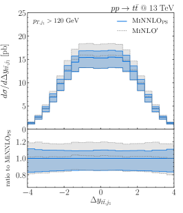
Figure 1: Distribution in the rapidity difference between the $t\bar{t}$ pair and the leading jet ($\Delta y_{t{\bar{t}},j_{1}}$), in the rapidity ($y_{t_{\rm av}}$) and the average transverse-momentum ($p_{T,t_{\rm av}}$) of the top and the anti-top, as well as in the rapidity ($y_{t\bar{t}}$), in the invariant mass ($m_{t\bar{t}}$) and in the transverse momentum ($p_{T,t\bar{t}}$) of the $t\bar{t}$ system. Predictions are shown for MiNNLO_PS (blue, solid), MiNLO^′ (black, dashed) and at NNLO (red, dashed). The black data points represent the CMS measurement at $13$ TeV of Ref. Sirunyan et al. (2018c), where the $y_{t_{\rm av}}$ and $p_{T,t_{\rm av}}$ distributions have been obtained with leptonically decaying top quarks.

In Fig. 1 we examine a set of differential distributions. To validate MiNNLO_PS, we compare it to the NNLO prediction without fiducial cuts, which could lead to significant differences due to the PS. Experimental data from the CMS collaboration unfolded and extrapolated to the inclusive phase space Sirunyan et al. (2018c), and divided by the appropriate branching fractions, are also shown. The top–left plot shows the rapidity difference between the $t{\bar{t}}$ system and the leading jet defined with $p_{T,\,j_{1}}\geq 120\,$GeV. Both MiNLO^′ and MiNNLO_PS are formally NLO accurate in this case, and the agreement between them indicates that this accuracy is retained by the MiNNLO_PS procedure. The same conclusion holds for other observables that require at least one resolved hard jet.

The distributions in the average top-quark rapidity ($y_{t_{\rm av}}$) and transverse momentum ($p_{T,t_{\rm av}}$) as well as in the invariant mass ($m_{t{\bar{t}}}$) and rapidity ($y_{t{\bar{t}}}$) of the $t{\bar{t}}$ pair shown in Fig. 1 are inclusive over QCD radiation. For such distributions MiNNLO_PS is expected to be NNLO accurate. Indeed, MiNNLO_PS and NNLO yield consistent results, with fully overlapping uncertainty bands. The small differences in the central value are once again due to the different treatment of terms beyond NNLO accuracy. The larger uncertainty bands of the MiNNLO_PS predictions are expected, since additional scale dependent terms are included within the first term in the r.h.s. of Eq. (11) that are not present in the fixed-order calculation. In comparison to the MiNLO^′ results the inclusion of NNLO corrections through MiNNLO_PS has an impact of about $10$%–$20$% on the differential distributions and substantially reduces the perturbative uncertainties. Also the agreement with data is quite remarkable. All data points are within one standard deviation from the MiNNLO_PS prediction, with the exception of the very first bin in the $m_{t{\bar{t}}}$ distribution that, on the other hand, is strongly affected by the finite width of the top, whose effects are not included here.

We finally discuss the transverse-momentum spectrum of the $t\bar{t}$ pair, denoted by $p_{T,\,{t\bar{t}}}$ in the bottom–right panel of Fig. 1. At large transverse momenta, the three predictions considered are effectively NLO accurate. Indeed, MiNLO^′ and MiNNLO_PS are essentially indistinguishable in that region, and at the same time consistent with the spectrum at fixed order. The small differences with NNLO are due to the generation of further radiation by the PS. At small transverse momenta, MiNNLO_PS induces ${\cal O}(10\%)$ corrections with respect to MiNLO^′ and significantly reduces the large scale dependence. In this region, it also differs in shape from the NNLO calculation, which diverges and becomes unphysical for vanishing transverse momenta. Within the relatively large experimental errors, MiNNLO_PS slightly improves the description of the data in terms of shape compared to NNLO for this observable.

In this letter we have presented the matching of the NNLO computation for top-quark pair production at hadron colliders with parton showers. This result has been obtained by constructing the MiNNLO_PS method for the production of heavy quarks, which constitutes the first NNLO+PS prediction for reactions with colour charges in the final state in hadronic collisions. The comparisons presented in Fig. 1 provide a numerical validation of MiNNLO_PS for top-quark pair production, demonstrating its NNLO accuracy. The simulations presented here also allow for the inclusion of the top-quark decay, paving the way to an accurate event generation for $t{\bar{t}}$ production at the LHC which will enable precise comparisons of fiducial measurements to theory.
Acknowledgements. We would like to thank Stefano Catani, Massimiliano Grazzini, and Keith Hamilton for discussions and comments on the manuscript. P.N. acknowledges support from Fondazione Cariplo and Regione Lombardia, grant 2017-2070, and from INFN.

Supplemental material

In this appendix we complement the results presented in the letter by comparing MiNNLO_PS, MiNLO^′, and NNLO predictions with different scale settings. In particular, we set $\mu_{R}^{(0)}=K_{R}\,m_{t\bar{t}}$ and $\mu_{0}=m_{t\bar{t}}\,e^{-L}$ for MiNNLO_PS and MiNLO^′, and we use $\mu_{0}=m_{t\bar{t}}$ for the NNLO fixed-order calculation. The other settings are as reported in the main text. Table 2 reports the total cross sections, while Fig. 2 shows the same distributions as shown in the letter, but with the updated scale setting. Despite the fact that higher-order differences are expected for all observables, we observe an excellent agreement between MiNNLO_PS and NNLO predictions for this scale choice.

MiNLO′	NNLO	MiNNLOPS
$\;\,572.9(2)_{-17\%}^{+21\%}$ pb	$\;\,719.1(8)_{-7.6\%}^{+7.0\%}$ pb	$\;\,719.8(2)_{-7.4\%}^{+7.6\%}$ pb

Table 2: The total $t\bar{t}$ cross section in different approximations. The quoted errors represent the scale uncertainty, while the numbers in brackets are the numerical uncertainty on the last digit.

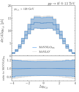
Figure 2: Same as Fig. 1, albeit without data and with the scale setting $\mu_{R}^{(0)}=K_{R}\,m_{t\bar{t}}$ and $\mu_{0}=m_{t\bar{t}}\,e^{-L}$ for MiNNLO_PS and MiNLO^′, and $\mu_{0}=m_{t\bar{t}}$ for NNLO.

References

- de Florian et al. (2016) D. de Florian et al. (LHC Higgs Cross Section Working Group), 2/2017 (2016), 10.23731/CYRM-2017-002, arXiv:1610.07922 [hep-ph] .
- Brivio et al. (2020) I. Brivio, S. Bruggisser, F. Maltoni, R. Moutafis, T. Plehn, E. Vryonidou, S. Westhoff, and C. Zhang, JHEP 02, 131 (2020), arXiv:1910.03606 [hep-ph] .
- Baak et al. (2014) M. Baak, J. Cúth, J. Haller, A. Hoecker, R. Kogler, K. Mönig, M. Schott, and J. Stelzer (Gfitter Group), Eur. Phys. J. C 74, 3046 (2014), arXiv:1407.3792 [hep-ph] .
- Degrassi et al. (2012) G. Degrassi, S. Di Vita, J. Elias-Miro, J. R. Espinosa, G. F. Giudice, G. Isidori, and A. Strumia, JHEP 08, 098 (2012), arXiv:1205.6497 [hep-ph] .
- Bärnreuther et al. (2012) P. Bärnreuther, M. Czakon, and A. Mitov, Phys. Rev. Lett. 109, 132001 (2012), arXiv:1204.5201 [hep-ph] .
- Czakon and Mitov (2012) M. Czakon and A. Mitov, JHEP 12, 054 (2012), arXiv:1207.0236 [hep-ph] .
- Czakon and Mitov (2013) M. Czakon and A. Mitov, JHEP 01, 080 (2013), arXiv:1210.6832 [hep-ph] .
- Czakon et al. (2013) M. Czakon, P. Fiedler, and A. Mitov, Phys. Rev. Lett. 110, 252004 (2013), arXiv:1303.6254 [hep-ph] .
- Czakon et al. (2016a) M. Czakon, D. Heymes, and A. Mitov, Phys. Rev. Lett. 116, 082003 (2016a), arXiv:1511.00549 [hep-ph] .
- Czakon et al. (2016b) M. Czakon, P. Fiedler, D. Heymes, and A. Mitov, JHEP 05, 034 (2016b), arXiv:1601.05375 [hep-ph] .
- Catani et al. (2019a) S. Catani, S. Devoto, M. Grazzini, S. Kallweit, J. Mazzitelli, and H. Sargsyan, Phys. Rev. D99, 051501 (2019a), arXiv:1901.04005 [hep-ph] .
- Catani et al. (2019b) S. Catani, S. Devoto, M. Grazzini, S. Kallweit, and J. Mazzitelli, JHEP 07, 100 (2019b), arXiv:1906.06535 [hep-ph] .
- Behring et al. (2019) A. Behring, M. Czakon, A. Mitov, A. S. Papanastasiou, and R. Poncelet, Phys. Rev. Lett. 123, 082001 (2019), arXiv:1901.05407 [hep-ph] .
- Beenakker et al. (1994) W. Beenakker, A. Denner, W. Hollik, R. Mertig, T. Sack, and D. Wackeroth, Nucl. Phys. B 411, 343 (1994).
- Bernreuther et al. (2006) W. Bernreuther, M. Fücker, and Z. Si, Phys. Lett. B 633, 54 (2006), [Erratum: Phys.Lett.B 644, 386–386 (2007)], arXiv:hep-ph/0508091 .
- Kuhn et al. (2007) J. H. Kuhn, A. Scharf, and P. Uwer, Eur. Phys. J. C 51, 37 (2007), arXiv:hep-ph/0610335 .
- Denner and Pellen (2016) A. Denner and M. Pellen, JHEP 08, 155 (2016), arXiv:1607.05571 [hep-ph] .
- Czakon et al. (2017) M. Czakon, D. Heymes, A. Mitov, D. Pagani, I. Tsinikos, and M. Zaro, JHEP 10, 186 (2017), arXiv:1705.04105 [hep-ph] .
- Zhu et al. (2013) H. X. Zhu, C. S. Li, H. T. Li, D. Y. Shao, and L. L. Yang, Phys. Rev. Lett. 110, 082001 (2013), arXiv:1208.5774 [hep-ph] .
- Li et al. (2013) H. T. Li, C. S. Li, D. Y. Shao, L. L. Yang, and H. X. Zhu, Phys. Rev. D 88, 074004 (2013), arXiv:1307.2464 [hep-ph] .
- Catani et al. (2014) S. Catani, M. Grazzini, and A. Torre, Nucl. Phys. B890, 518 (2014), arXiv:1408.4564 [hep-ph] .
- Catani et al. (2018) S. Catani, M. Grazzini, and H. Sargsyan, JHEP 11, 061 (2018), arXiv:1806.01601 [hep-ph] .
- Beneke et al. (2012a) M. Beneke, P. Falgari, S. Klein, and C. Schwinn, Nucl. Phys. B 855, 695 (2012a), arXiv:1109.1536 [hep-ph] .
- Beneke et al. (2012b) M. Beneke, P. Falgari, S. Klein, J. Piclum, C. Schwinn, M. Ubiali, and F. Yan, JHEP 07, 194 (2012b), arXiv:1206.2454 [hep-ph] .
- Ju et al. (2020) W.-L. Ju, G. Wang, X. Wang, X. Xu, Y. Xu, and L. L. Yang, JHEP 06, 158 (2020), arXiv:2004.03088 [hep-ph] .
- Czakon et al. (2020) M. L. Czakon et al., Chin. Phys. C 44, 083104 (2020), arXiv:1901.08281 [hep-ph] .
- Nason (2019) P. Nason, “The Top Mass in Hadronic Collisions,” in From My Vast Repertoire …: Guido Altarelli’s Legacy, edited by A. Levy, S. Forte, and G. Ridolfi (2019) pp. 123–151, arXiv:1712.02796 [hep-ph] .
- Hoang (2020) A. H. Hoang, (2020), 10.1146/annurev-nucl-101918-023530, arXiv:2004.12915 [hep-ph] .
- Beneke et al. (2017) M. Beneke, P. Marquard, P. Nason, and M. Steinhauser, Phys. Lett. B 775, 63 (2017), arXiv:1605.03609 [hep-ph] .
- Hoang et al. (2017) A. H. Hoang, C. Lepenik, and M. Preisser, JHEP 09, 099 (2017), arXiv:1706.08526 [hep-ph] .
- Hoang et al. (2018) A. H. Hoang, S. Plätzer, and D. Samitz, JHEP 10, 200 (2018), arXiv:1807.06617 [hep-ph] .
- Ferrario Ravasio et al. (2019) S. Ferrario Ravasio, P. Nason, and C. Oleari, JHEP 01, 203 (2019), arXiv:1810.10931 [hep-ph] .
- Aad et al. (2020a) G. Aad et al. (ATLAS), Phys. Lett. B 810, 135797 (2020a), arXiv:2006.13076 [hep-ex] .
- Aad et al. (2020b) G. Aad et al. (ATLAS), (2020b), arXiv:2006.09274 [hep-ex] .
- Aad et al. (2020c) G. Aad et al. (ATLAS), Eur. Phys. J. C 80, 528 (2020c), arXiv:1910.08819 [hep-ex] .
- Aad et al. (2019a) G. Aad et al. (ATLAS), Eur. Phys. J. C 79, 1028 (2019a), arXiv:1908.07305 [hep-ex] .
- Khachatryan et al. (2017) V. Khachatryan et al. (CMS), Eur. Phys. J. C 77, 172 (2017), arXiv:1611.04040 [hep-ex] .
- Sirunyan et al. (2017) A. M. Sirunyan et al. (CMS), JHEP 09, 051 (2017), arXiv:1701.06228 [hep-ex] .
- Sirunyan et al. (2019a) A. M. Sirunyan et al. (CMS), JHEP 02, 149 (2019a), arXiv:1811.06625 [hep-ex] .
- Sirunyan et al. (2018a) A. Sirunyan et al. (CMS), JHEP 06, 002 (2018a), arXiv:1803.03991 [hep-ex] .
- Sirunyan et al. (2018b) A. Sirunyan et al. (CMS), JHEP 04, 060 (2018b), arXiv:1708.07638 [hep-ex] .
- Chatrchyan et al. (2014) S. Chatrchyan et al. (CMS), Phys. Lett. B 728, 496 (2014), [Erratum: Phys.Lett.B 738, 526–528 (2014)], arXiv:1307.1907 [hep-ex] .
- Klijnsma et al. (2017) T. Klijnsma, S. Bethke, G. Dissertori, and G. P. Salam, Eur. Phys. J. C 77, 778 (2017), arXiv:1708.07495 [hep-ph] .
- Sirunyan et al. (2020a) A. M. Sirunyan et al. (CMS), Eur. Phys. J. C 80, 658 (2020a), arXiv:1904.05237 [hep-ex] .
- Aad et al. (2019b) G. Aad et al. (ATLAS), JHEP 11, 150 (2019b), arXiv:1905.02302 [hep-ex] .
- Sirunyan et al. (2020b) A. M. Sirunyan et al. (CMS), (2020b), arXiv:2009.07123 [hep-ex] .
- Sirunyan et al. (2019b) A. M. Sirunyan et al. (CMS), Phys. Rev. D 100, 072007 (2019b), arXiv:1907.01590 [hep-ex] .
- Cooper-Sarkar et al. (2020) A. M. Cooper-Sarkar, M. Czakon, M. A. Lim, A. Mitov, and A. S. Papanastasiou, (2020), arXiv:2010.04171 [hep-ph] .
- Buckley et al. (2011) A. Buckley et al., Phys. Rept. 504, 145 (2011), arXiv:1101.2599 [hep-ph] .
- Frederix and Frixione (2012) R. Frederix and S. Frixione, JHEP 12, 061 (2012), arXiv:1209.6215 [hep-ph] .
- Hoeche et al. (2015) S. Hoeche, F. Krauss, P. Maierhoefer, S. Pozzorini, M. Schonherr, and F. Siegert, Phys. Lett. B 748, 74 (2015), arXiv:1402.6293 [hep-ph] .
- Cormier et al. (2019) K. Cormier, S. Plätzer, C. Reuschle, P. Richardson, and S. Webster, Eur. Phys. J. C 79, 915 (2019), arXiv:1810.06493 [hep-ph] .
- Ježo and Nason (2015) T. Ježo and P. Nason, JHEP 12, 065 (2015), arXiv:1509.09071 [hep-ph] .
- Ježo et al. (2016) T. Ježo, J. M. Lindert, P. Nason, C. Oleari, and S. Pozzorini, Eur. Phys. J. C 76, 691 (2016), arXiv:1607.04538 [hep-ph] .
- Frederix et al. (2016) R. Frederix, S. Frixione, A. S. Papanastasiou, S. Prestel, and P. Torrielli, JHEP 06, 027 (2016), arXiv:1603.01178 [hep-ph] .
- Höche et al. (2017) S. Höche, F. Krauss, and S. Prestel, JHEP 10, 093 (2017), arXiv:1705.00982 [hep-ph] .
- Dulat et al. (2018) F. Dulat, S. Höche, and S. Prestel, Phys. Rev. D 98, 074013 (2018), arXiv:1805.03757 [hep-ph] .
- Dasgupta et al. (2018) M. Dasgupta, F. A. Dreyer, K. Hamilton, P. F. Monni, and G. P. Salam, JHEP 09, 033 (2018), arXiv:1805.09327 [hep-ph] .
- Bewick et al. (2020) G. Bewick, S. Ferrario Ravasio, P. Richardson, and M. H. Seymour, JHEP 04, 019 (2020), arXiv:1904.11866 [hep-ph] .
- Dasgupta et al. (2020) M. Dasgupta, F. A. Dreyer, K. Hamilton, P. F. Monni, G. P. Salam, and G. Soyez, Phys. Rev. Lett. 125, 052002 (2020), arXiv:2002.11114 [hep-ph] .
- Forshaw et al. (2020) J. R. Forshaw, J. Holguin, and S. Plätzer, JHEP 09, 014 (2020), arXiv:2003.06400 [hep-ph] .
- Hamilton et al. (2020) K. Hamilton, R. Medves, G. P. Salam, L. Scyboz, and G. Soyez, (2020), arXiv:2011.10054 [hep-ph] .
- Hamilton et al. (2013) K. Hamilton, P. Nason, C. Oleari, and G. Zanderighi, JHEP 05, 082 (2013), arXiv:1212.4504 [hep-ph] .
- Alioli et al. (2014) S. Alioli, C. W. Bauer, C. Berggren, F. J. Tackmann, J. R. Walsh, and S. Zuberi, JHEP 06, 089 (2014), arXiv:1311.0286 [hep-ph] .
- Höche et al. (2015) S. Höche, Y. Li, and S. Prestel, Phys. Rev. D 91, 074015 (2015), arXiv:1405.3607 [hep-ph] .
- Monni et al. (2020a) P. F. Monni, P. Nason, E. Re, M. Wiesemann, and G. Zanderighi, JHEP 05, 143 (2020a), arXiv:1908.06987 [hep-ph] .
- Monni et al. (2020b) P. F. Monni, E. Re, and M. Wiesemann, Eur. Phys. J. C 80, 1075 (2020b), arXiv:2006.04133 [hep-ph] .
- Nason (2004) P. Nason, JHEP 11, 040 (2004), arXiv:hep-ph/0409146 [hep-ph] .
- Nason and Ridolfi (2006) P. Nason and G. Ridolfi, JHEP 08, 077 (2006), arXiv:hep-ph/0606275 [hep-ph] .
- Frixione et al. (2007) S. Frixione, P. Nason, and C. Oleari, JHEP 11, 070 (2007), arXiv:0709.2092 [hep-ph] .
- Alioli et al. (2010) S. Alioli, P. Nason, C. Oleari, and E. Re, JHEP 06, 043 (2010), arXiv:1002.2581 [hep-ph] .
- Catani and Grazzini (2011) S. Catani and M. Grazzini, Nucl. Phys. B845, 297 (2011), arXiv:1011.3918 [hep-ph] .
- Catani and Seymour (1997) S. Catani and M. Seymour, Nucl. Phys. B485, 291 (1997), arXiv:hep-ph/9605323 [hep-ph] .
- Bozzi et al. (2006) G. Bozzi, S. Catani, D. de Florian, and M. Grazzini, Nucl. Phys. B737, 73 (2006), arXiv:hep-ph/0508068 [hep-ph] .
- Czakon (2008) M. Czakon, Phys. Lett. B 664, 307 (2008), arXiv:0803.1400 [hep-ph] .
- Catani and Grazzini (2012) S. Catani and M. Grazzini, Eur. Phys. J. C72, 2013 (2012), [Erratum: Eur. Phys. J.C72,2132(2012)], arXiv:1106.4652 [hep-ph] .
- Czakon and Mitov (2014) M. Czakon and A. Mitov, Comput. Phys. Commun. 185, 2930 (2014), arXiv:1112.5675 [hep-ph] .
- Catani et al. (2012) S. Catani, L. Cieri, D. de Florian, G. Ferrera, and M. Grazzini, Eur.Phys.J. C72, 2195 (2012), arXiv:1209.0158 [hep-ph] .
- Gehrmann et al. (2012) T. Gehrmann, T. Lübbert, and L. L. Yang, Phys. Rev. Lett. 109, 242003 (2012), arXiv:1209.0682 [hep-ph] .
- Bärnreuther et al. (2014) P. Bärnreuther, M. Czakon, and P. Fiedler, JHEP 02, 078 (2014), arXiv:1312.6279 [hep-ph] .
- Gehrmann et al. (2014) T. Gehrmann, T. Luebbert, and L. L. Yang, JHEP 06, 155 (2014), arXiv:1403.6451 [hep-ph] .
- Echevarria et al. (2016) M. G. Echevarria, I. Scimemi, and A. Vladimirov, JHEP 09, 004 (2016), arXiv:1604.07869 [hep-ph] .
- Angeles-Martinez et al. (2018) R. Angeles-Martinez, M. Czakon, and S. Sapeta, JHEP 10, 201 (2018), arXiv:1809.01459 [hep-ph] .
- Luo et al. (2020) M.-X. Luo, T.-Z. Yang, H. X. Zhu, and Y. J. Zhu, JHEP 01, 040 (2020), arXiv:1909.13820 [hep-ph] .
- Luo et al. (2019) M.-X. Luo, X. Wang, X. Xu, L. L. Yang, T.-Z. Yang, and H. X. Zhu, JHEP 10, 083 (2019), arXiv:1908.03831 [hep-ph] .
- (86) S. Catani, S. Devoto, M. Grazzini, and J. Mazzitelli, In preparation .
- (87) H. Sargsyan, https://doi.org/10.5167/uzh-142437, Ph.D. Thesis (University of Zurich) .
- Hamilton et al. (2012) K. Hamilton, P. Nason, and G. Zanderighi, JHEP 10, 155 (2012), arXiv:1206.3572 [hep-ph] .
- Alioli et al. (2012) S. Alioli, S.-O. Moch, and P. Uwer, JHEP 01, 137 (2012), arXiv:1110.5251 [hep-ph] .
- Sjostrand and Skands (2005) T. Sjostrand and P. Z. Skands, Eur. Phys. J. C 39, 129 (2005), arXiv:hep-ph/0408302 .
- Catani et al. (1991) S. Catani, B. R. Webber, and G. Marchesini, Nucl. Phys. B349, 635 (1991).
- Ball et al. (2017) R. D. Ball et al. (NNPDF), Eur. Phys. J. C77, 663 (2017), arXiv:1706.00428 [hep-ph] .
- Banfi et al. (2012a) A. Banfi, G. P. Salam, and G. Zanderighi, JHEP 06, 159 (2012a), arXiv:1203.5773 [hep-ph] .
- Banfi et al. (2012b) A. Banfi, P. F. Monni, G. P. Salam, and G. Zanderighi, Phys. Rev. Lett. 109, 202001 (2012b), arXiv:1206.4998 [hep-ph] .
- Monni et al. (2016) P. F. Monni, E. Re, and P. Torrielli, Phys. Rev. Lett. 116, 242001 (2016), arXiv:1604.02191 [hep-ph] .
- Bizon et al. (2018) W. Bizon, P. F. Monni, E. Re, L. Rottoli, and P. Torrielli, JHEP 02, 108 (2018), arXiv:1705.09127 [hep-ph] .
- Mazzitelli et al. (2021) J. Mazzitelli, P. Monni, P. Nason, E. Re, M. Wiesemann, and G. Zanderighi, Supplemental material attached to the arXiv version of this letter (2021).
- Grazzini et al. (2018) M. Grazzini, S. Kallweit, and M. Wiesemann, Eur. Phys. J. C78, 537 (2018), arXiv:1711.06631 [hep-ph] .
- Sirunyan et al. (2018c) A. M. Sirunyan et al. (CMS), Phys. Rev. D 97, 112003 (2018c), arXiv:1803.08856 [hep-ex] .