Lifelong Learning in Multi-Armed Bandits

Abstract

Continuously learning and leveraging the knowledge accumulated from prior tasks in order to improve future performance is a long standing machine learning problem. In this paper, we study the problem in the multi-armed bandit framework with the objective to minimize the total regret incurred over a series of tasks. While most bandit algorithms are designed to have a low worst-case regret, we examine here the average regret over bandit instances drawn from some prior distribution which may change over time. We specifically focus on confidence interval tuning of UCB algorithms. We propose a bandit over bandit approach with greedy algorithms and we perform extensive experimental evaluations in both stationary and non-stationary environments. We further apply our solution to the mortal bandit problem, showing empirical improvement over previous work.

1 Introduction

The multi-armed bandit (MAB) is a simple instance of online learning problem with partial feedback (see [13]; [34]; [44], and references therein). In the stochastic bandit framework, a learning agent sequentially pulls arms and obtains noisy rewards. The goal of the agent is to maximize her expected cumulative reward, or equivalently, to minimize her regret, which is the difference between the cumulative reward of an oracle (that knows the mean rewards of arms) and the one of the agent. There is thus a clear trade-off, called “exploration vs exploitation”, that arises between gathering information on uncertain arms by pulling them (exploration) and leveraging the information obtained so far by greedily pulling the arm with the highest estimated reward (exploitation). MAB has received a large attention recently due to its wide applications range and the theoretical guarantees associated with learning algorithms (see also [9], and references therein for a survey on practical applications of MAB).

Most of the work in the stochastic bandit literature focuses on developing algorithms with optimal regret, either asymptotically in the instance-dependent sense or in the worst-case, on some problem class (typically on bounded or subgaussian rewards). While the theory guarantees that these algorithms will have a sublinear regret in all instances within the problem class, they will be overly conservative for the majority of these instances, leading to a large regret. Additionally, on these “easier” instances, sophisticated algorithms are outperformed by simpler ones [48, 31], which is an obstacle to their implementation in practice. In this paper, we consider that the learner successively interacts with a task sampled from a problem class with some prior distribution, which may or may not be stationary over time. Within each task, there is a learning problem which is a MAB problem with a fixed time horizon. The learning agent does not know the model parameters of each bandit problem, nor does she know the prior distribution within the problem class. Yet, it is critical for the learner be to able to “track” this probability distribution to build lifelong learning agent and thus achieve the best possible performance. In a stationary environment, the learner experiences the same bandit problem over and over again, and an efficient algorithm, in order to improve the performance when it faces the same problem again, should leverage the information acquired from previous tasks. Conversely in a non-stationary environment, the distribution within the problem class may change over time and the previously learned solution may fail to keep its good performance under the new distribution. An efficient algorithm must thus continuously learn to improve itself. The goal of the learning agent is then to minimize the lifelong regret, that is the cumulative regret across all tasks. This approach can be regarded as a special case of meta-learning [42, 46] or lifelong learning [45, 16, 43].

Our results

We focus on a tractable instance of this problem that is the tuning of the confidence interval width of UCB-like policies. We first evaluate the impact of the choice of algorithm on empirical performance over several problem classes with different prior and different number of arms. On a side note, we prove a bound on the Bayesian regret of a tuned UCB algorithm showing that we do not lose all theoretical guarantees. We then concentrate on learning in a stationary environment. We first investigate the influence of various initializations on performance. Next, we discuss about the main part of this paper that is learning the optimal algorithm. For this purpose, we consider a bandit over bandit approach, that is using a bandit algorithm to choose the optimal parameter. We show empirically that the Greedy algorithm as the meta-algorithm performs extremely well. We next concentrate on learning in a non-stationary environment, precisely we look at both an abruptly changing and a slowly changing environment. To this effect, we adapt the Greedy algorithm using methods from non-stationary bandits. Finally, we apply our method to a more realistic setting, the mortal bandit problem. By decomposing the time horizon into episodes according to the expected lifetime of arms, we show great empirical improvement compared to previous work.

Related Work

Bayesian bandits [23, 24, 7] have been studied extensively with the goal of developing optimal algorithms in the Bayesian sense. Lower bounds on the Bayesian regret have also been derived [32, 28]. Unfortunately, computing the Bayesian optimal algorithm is generally intractable [34].

The closest to our work is that of [35] who considered a framework which closely resembles to ours except they studied the stochastic setting and further assumed a finite set of models; whereas we consider the Bayesian setting and do not make any assumption on the number of changes in the prior distribution. [20] extended the previous work in the contextual framework.

Also related to our work, [37] tuned existing algorithms and also learned index algorithms of historical features. [26] proposed a best-arm identification algorithm for tuning the confidence interval of the UCB algorithm and the posterior distribution of the Thompson Sampling algorithm. [12] focused on “differentiable” algorithms and optimized them by gradient ascent. In comparison, the setting of these works are offline while we are more interested in the lifelong regret incurred in potentially non-stationary environments.

Several works also use bandit algorithms as meta-algorithm. [36] introduced a bandit-based approach to hyperparameter optimization using Sequential Halving, a pure-exploration bandit algorithm, as a subroutine. The celebrated UCT algorithm [30] makes use of the UCB algorithm applies on trees. In the non-stationary framework, a few methods involve MAB in a hierarchical way: [25] considered a meta-bandit to decide whether to accept the change detection or not; [17] used the EXP3 algorithm to decide the window size of the SW-UCB algorithm; and [49, 50] adopted a hierarchical bandit algorithm where a master bandit manages some slave bandits.

The model can also be viewed as a special case of mortal bandits [14, 8, 47] in which arms show up by batch where the time of death is the same for each arm in a given batch.

2 Setting

In the stochastic MAB model, an agent interacts sequentially with a set of $K$ unknown distributions $\mathcal{V}_{1},\dots,\mathcal{V}_{K}$, called arms. At time $t$, the agent chooses an arm $A_{t}$ which yields a reward $X_{t}$ drawn from the associated probability distribution $\mathcal{V}_{A_{t}}$. The objective is to design a sequential algorithm maximizing the expected cumulative reward up to some time horizon $T$. Let $\mu_{1},\dots,\mu_{K}$ denote the mean rewards of arms, and $\mu^{\star}\coloneqq\max_{k\in[K]}\mu_{k}$. The goal is equivalent to minimizing the regret, defined as the difference between the expected reward accumulated by an oracle strategy always playing the best arm at each round, and the one accumulated by an algorithm $\mathcal{A}$,

$$R(T,\mathcal{A})=\mathbb{E}\left[\sum_{t=1}^{T}\left(\mu^{\star}-\mu_{A_{t}}\right)\right]$$

where the expectation is taken with respect to the randomness in the sequence of successive rewards from each arm and the possible randomization of the algorithm. Furthermore, we assume the following Bayesian, parametric bandit setting: a random vector $\boldsymbol{\theta}=\left(\theta_{1},\dots,\theta_{K}\right)$ is drawn from a prior distribution $\Pi$, and the distribution of arm $k$ depends on the parameter $\theta_{k}$. This leads to the notion of Bayesian regret which depends on the prior distribution $\Pi$,

$$\mathrm{BR}_{\Pi}(T,\mathcal{A})=\int R(T,\mathcal{A})d\Pi(\boldsymbol{\theta})\,.$$

We consider a lifelong learning setting where at each episode $j$ the learner interacts with a task $\mathcal{V}_{\theta_{1}^{j}},\dots,\mathcal{V}_{\theta_{K}^{j}}$, where each $\theta_{k}^{j}$ is drawn i.i.d. from a prior distribution $\Pi_{j}$. The objective is to find a series of algorithms minimizing the lifelong (Bayesian) regret over $J$ episodes,

$$\mathrm{LR}_{\boldsymbol{\Pi}}(T,\mathfrak{A})=\sum_{j=1}^{J}\mathrm{BR}_{\Pi_{j}}(T,\mathcal{A}_{j})$$

where $\mathfrak{A}=\left(\mathcal{A}_{1},\dots,\mathcal{A}_{J}\right)$ and $\boldsymbol{\Pi}=\left(\Pi_{1},\dots,\Pi_{J}\right)$ denote respectively the algorithms and the prior distributions for each episode. We further assume that the horizon for each task $T$ and the number of episodes $J$ are known. An unknown number of episodes can be handled as usual [18]; while the knowledge of the time horizon is mostly for convenience in the choice of the sub-algorithm and similar results can be achieved with an anytime algorithm.

In order to minimize the lifelong regret, our method consists in designing a meta-algorithm which, at each episode $j$, selects an algorithm $\mathcal{A}_{j}$ from a class of algorithms, which can be finite or infinite, that aims at minimizing the Bayesian regret with respect to the prior distribution $\Pi_{j}$.

We especially focus on a tractable class of algorithms, the UCB algorithm [3] with a parameter $\gamma$ controlling the width of the confidence interval. We emphasis that similar results can be obtained with any UCB-like algorithms. Formally, the UCB($\gamma$) index of arm $k\in[K]$ in round $t$ is

$$U_{t}(k)=\widehat{\mu}_{k}(t-1)+\gamma\sqrt{\frac{2\log\left(1/\delta\right)}{N_{k}(t-1)}}$$

where $\widehat{\mu}_{k}(t)$ is the average reward of arm $k$ in the first $t$ rounds, $N_{k}(t)$ is the number of times that arm $k$ has been pulled in the first $t$ rounds and $\delta=1/T$ is the probability that the confidence interval fails (in subsequent sections, we will choose $\delta=1/T$). Note that the case $\gamma=1$ corresponds to the theoretical value that attains the optimal instance-dependent regret for Gaussian rewards, while $\gamma=0$ corresponds to the Greedy algorithm. Hence for this class of algorithms, the meta-algorithm faces a new trade-off between being conservative and being aggressive on a class of bandit instances. Thereby, the objective that is to minimize the lifelong regret is equivalent to finding the optimal values of $\gamma\in[0,1]$ that minimizes the Bayesian regret in each episode.

Theoretically, any worst-case optimal algorithm will also be optimal, up to constant factors, in the Bayesian setting [34]; and thus optimal in the lifelong setting. Yet, we will see that we can empirically improve these algorithms. We end this section with an analysis of this tuned UCB. More generally, [41] noticed that the Bayesian regret of any UCB-like algorithm satisfies

$$\mathrm{BR}_{\Pi}(T,\textsc{UCB})\leq\mathbb{E}\left[\sum_{t=1}^{T}\left(\mu^{\star}-U_{t}(A^{\star})\right)+\sum_{t=1}^{T}\left(U_{t}(A_{t})-\mu_{A_{t}}\right)\right]$$ (1)

where $A^{\star}$ denotes the optimal arm, which is a random variable. Specifically for the UCB($\gamma$) algorithm we state the following theorem.

Theorem 1.

For 1-subgaussian distributions with mean in $[0,1]$, UCB($\gamma$) with $\gamma>0$ satisfies

$$\mathrm{BR}_{\Pi}(T,\textsc{UCB}(\gamma))\leq 4KT^{2}\delta^{4\gamma^{2}}+2\gamma\sqrt{2KT\log(1/\delta)}\,.$$

As an example, for $\gamma=1$ and $\delta=1/T$, we get the known bound $\mathcal{O}\left(\sqrt{KT\log{}T}\right)$.

Proof.

Let $E$ be the event that for all $t=1,\ldots,T$ and $k=1,\ldots,K$,

$$\left|\widehat{\mu}_{k}(t-1)-\mu_{k}\right|<\gamma\sqrt{\frac{2\log(1/\delta)}{N_{k}(t-1)}}\,.$$

Using the subgaussian assumption and a union bound, we get that $\mathbb{P}\left(E^{c}\right)\leq 2KT\delta^{4\gamma^{2}}$. On the event $E^{c}$, the terms inside the expectation of Equation (1) are bounded by $2T$, while on the event $E$, the first sum is bounded by 0 and for the second term, standard computations yield

$$\sum_{t=1}^{T}\left(U_{t}(A_{t})-\mu_{A_{t}}\right)\mathbf{1}\{E\}\leq 2\gamma\sqrt{2KT\log(1/\delta)}\,.$$

Putting together the pieces completes the proof. ∎

3 Choice of the class of algorithms

We begin by showing that the choice of the class of algorithms in which we seek to find the one that maximize the average cumulative reward over bandit instances, is of the utmost importance in order to have the best possible empirical performance, and the most favorable algorithm depends on a number of factors. In Figure 1, we evaluate the Bayesian regret of several UCB-like algorithms as a function of their parameter $\gamma$ in different setups. In all experiments, the distribution of each arm is a Bernoulli distribution where the mean reward is drawn i.i.d. from a uniform distribution over $[0,1]$. The horizon is fixed at $T=1000$ and we vary the number of arms $K$. Results are averaged over $5000$ iterations. See also Appendix A.1 for additional experiments with different distributions and priors.

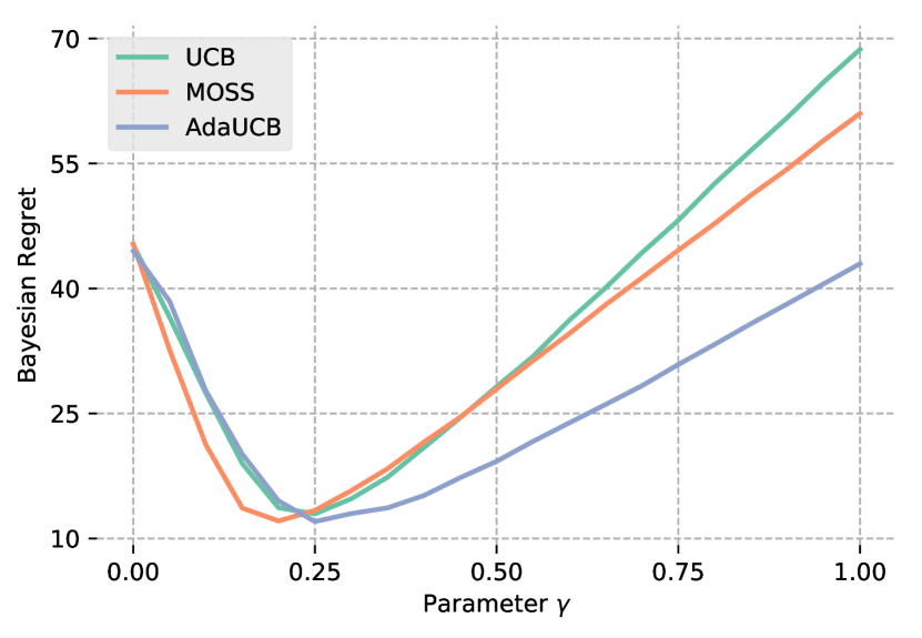
(a) $K=5$

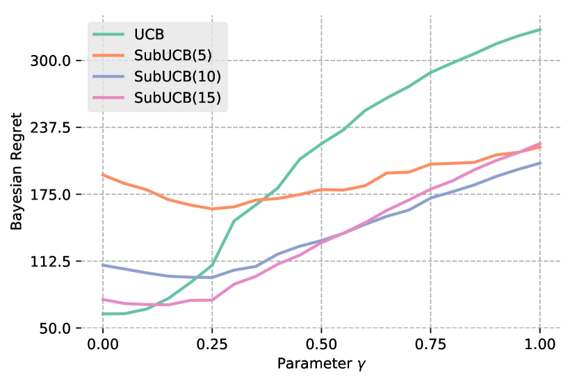
(b) $K=63$

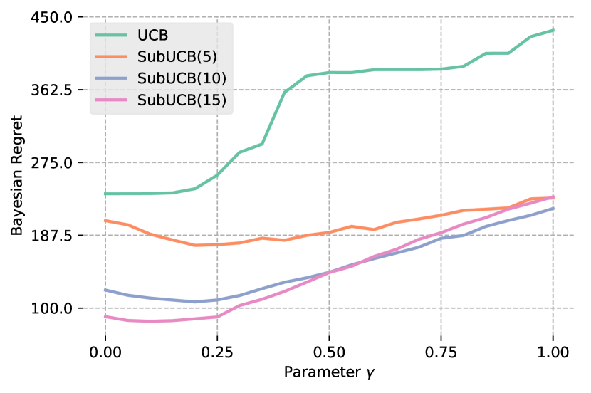
(c) $K=250$

Figure 1: Bayesian regret of various algorithms as a function of $\gamma$ for diverse numbers of arms $K$.

In Figure 1(a), we compare, for a small number of arms $K$, different UCB-like algorithms: the original UCB algorithm [3], MOSS [2], which is known to be worst-case optimal contrary to UCB, and AdaUCB [33] which is simultaneously worst-case optimal, asymptotically optimal, and never worse than UCB in the worst case. Interestingly, the later statement is also verified on the Bayesian regret for all values of $\gamma$. The same can also be said almost everywhere for MOSS over UCB. For large values of $\gamma$, AdaUCB outperforms MOSS while for small values, MOSS only improves slightly over AdaUCB. As a result, if one is purely interested in great empirical performance, a default choice would be AdaUCB for any value of $\gamma$. However in the lifelong setting, we want to optimize the parameter $\gamma$ and it is not clear which choice of algorithm will perform better through all the episodes; AdaUCB may be better but this also makes it harder for the meta-algorithm to find the optimal value of $\gamma$, meaning a potentially larger lifelong regret compared to UCB for example. Additionally, the best Bayesian regret of the optimally tuned version of each algorithm is roughly the same for all three. Hence our choice of the UCB algorithm, which is simple enough for illustration, yet may also be suitable for practical applications. We finally note that for all algorithms, the gain of their tuned version over the default choice ($\gamma=1$) is substantial even though MOSS and AdaUCB are worst-case optimal up to constant factors, supporting our choice to optimize algorithms for practical purpose.

In Figure 1(b) and 1(c), we compare the UCB algorithm with sub-sampled versions of itself, denoted SubUCB, in the case of an intermediate and a large number of arms $K$. Formally, SubUCB($m$) selects randomly $m$ arms and performs UCB on these arms. For $K=63$, we see that the Greedy algorithm, symbolized by UCB with $\gamma=0$, performs better than any tuned UCB and also better than SubUCB. For $K=250$, SubUCB performs always better than UCB. It is interesting to notice that as $m$ grows larger, up to a certain point, SubUCB has a better optimal Bayesian regret, becomes more sensitive to the parameter $\gamma$ and a sub-sampled version of the Greedy algorithm turns into the best performing algorithm. We mention that these behaviors, i.e. the good empirical performance of the Greedy algorithm and the superiority of a sub-sampled version of UCB in the case of a great number of arms, have been pointed out by [6]. We showed that they also hold true empirically after tuning of the confidence interval width.

4 Learning in a stationary environment

In this section, we consider the learning of the optimal algorithm in a fixed environment, i.e. when the prior distribution is the same in all episodes. In this case, the objective is equivalent to finding the algorithm that minimizes the Bayesian regret for that specific prior distribution.

4.1 Influence of the initialization

We start with a study of the effect of the initialization choice on empirical performance. By default, most bandit algorithms initialize arms by pulling them at least one time. Knowing that we solve again and again similar bandit problems, we may want to find a more clever initialization. For example, consider a challenging bandit problem with a large number of arms with respect to the time horizon and assume we have found a reasonably good arm; exploiting this arm may then be more rewarding that exploring new arms in the hope of finding a better one. This becomes especially critical the more greedy we get. In this section, we fix the value of the hyperparameter $\gamma$ and we evaluate three different initializations. In all cases, we set the empirical means of arms to a specific value and their upper confidence bounds are built as if they have been played once. In the first case we set this value at 0 (Init 1), in the second (Init 2) and third (Init 3) cases, it is fixed at the mean and median, respectively, of previous empirical means. We denote by “Init 0” the default initialization.

We analyze here a particular problem class and we refer the reader to Appendix A.2 for a more complete overview on the impact of the different initializations for different prior distributions and number of arms. In this experiment, each episode consists of a Gaussian bandit problem with $K=5$ arms, a time horizon $T=,000$ and the mean rewards of arms are drawn i.i.d. from a uniform distribution over $[0,1]$. We fix $\gamma=0.2$ and we repeat this tuned UCB for $J=100$ episodes with the different initializations previously mentioned. On Figure 2(a), we report the lifelong regret averaged over 100 iterations.

In this experiment, all three initializations improve over the default choice; it turns out that initializing arms with the median of previous empirical means performs better than the mean of previous arms which in turn performs better than an initialization at 0. However, this is not always the case and it heavily depends on the number of arms $K$ and on the prior distribution. Fortunately, this choice is insignificant on instances with a small number of arms, which we study in this paper, therefore in what follows we assume that UCB uses the default initialization in each episode.

(a) Comparison of various initializations

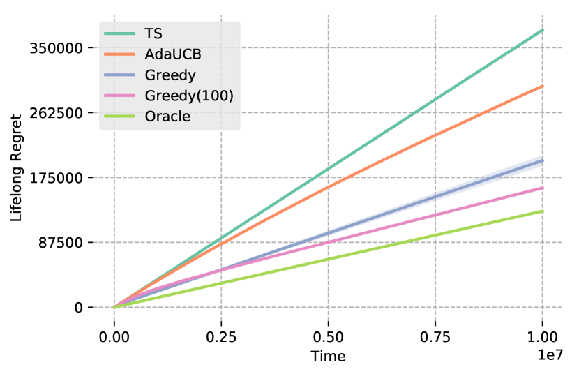
(b) Comparison of various meta-algorithms

Figure 2: Lifelong regret of various meta-algorithms in stationary environments. Shaded areas show standard errors.

4.2 Bandit algorithms as meta-algorithm

Now that the initialization rule is set, we can focus on the meta-algorithm, i.e. the algorithm that is responsible for picking the parameter $\gamma$ of UCB for each episode, and ultimately, is the keystone in the minimization of the lifelong regret. We consider bandit algorithms for the choice of the meta-algorithm, since they are efficient online optimization algorithms. This may seem like a vicious circle as we are talking about optimization of bandits algorithms and we want to avoid having to optimize the optimizer. Fortunately, the two algorithms, the meta-algorithm and the sub-algorithm, face a different problem. Indeed, the sub-algorithm aims at maximizing the average reward over bandit instances while the meta-algorithm aims at maximizing a function, which is the expected cumulative reward of the sub-algorithm with respect to its parameter $\gamma$. The dilemma encountered by the meta-algorithm is actually a continuous-armed bandit problem [29, 4] where the set of arms lies in some bounded interval, in our case the different $\gamma\in[0,1]$. [29] proposed a simple, yet nearly optimal, algorithm which consists in discretizing the $[0,1]$ interval into a finite set of $n$ equally spaced points and running a standard bandit algorithm over those points. Unfortunately, their theoretical result holds only when the function to be optimize satisfies some Hölder conditions which may not verified for the Bayesian regret of UCB($\gamma$). Still, that does not refrain us from using this strategy. The chosen number of arms $n$ is critical in practice; set too low we may be far from the optimal solution and set too high we may end up exploring all the time. [4], with a similar algorithm, claimed a value $n=(J/\log J)^{1/3}$ is optimal without knowing the exact Hölder condition. We thus choose this specific discretization in our simulations. It has also been noted by [6] that the Greedy algorithm, known to have a linear regret, ran with a sufficiently large number of arms may benefit from “free” exploration. This change point in its behavior happens around $\sqrt{J}$; we also evaluate Greedy with a discretization which contains that many points.

We again study a particular bandit instance; see Appendix A.3 for the same experiment made with different choices of prior distribution. In this experiment, each episode consists of a Bernoulli bandit problem with $K=5$ arms, a time horizon $T=1000$ and the mean rewards are drawn i.i.d. from a uniform distribution over $[0,1]$. We set the number of episodes $J=10000$ and we compare different meta-algorithms, namely Thompson Sampling (TS) with a uniform prior [1], AdaUCB [33] and the Greedy algorithm with the two discussed discretizations, denoted Greedy(100) for the discretization with 100 points. We also report an oracle meta-algorithm, which knows the optimal $\gamma$. Results are averaged over 100 iterations and are displayed on Figure 2(b).

We see that TS has a “linear” regret indicating that it fails to learn a good parameter $\gamma$ within that time frame. Whereas the regret of AdaUCB is sublinear and the algorithm is thus learning; however it is outperformed for a relatively long period of time by a naive Greedy, which is stuck to a suboptimal, yet good arm. The most interesting part is that Greedy(100) performs extremely well; its regret is remarkably close to the one of Oracle and is even sublinear. This supports the notion of free exploration for a large enough number of arms of the Greedy algorithm.

5 Leaning in a non-stationary environment

We now focus our attention to learning in a non-stationary environment, i.e. in which the prior distribution is not the same for all episodes. We will consider two scenarios: one where the environment changes abruptly and another where it slowly changes over time. Regrettably, adaptively tracking the prior distribution is intractable without making strong distributional assumptions (and potentially at the cost of forced exploration). Nonetheless, that does not mean that trying to improve over a naive meta-algorithm is hopeless. Taking inspiration from the stochastic non-stationary bandit literature [22], we adapt the index of Greedy to take into account a changing environment.

The following two adjustments are based on the idea of “forgetting” rewards obtained long ago. The first one is based on discounting. Formally, let $\omega\in(0,1)$ be the discount factor and define the discounted DGreedy index

$$\widehat{\mu}_{k}^{\omega}(t)=\frac{\sum_{s=1}^{t}\omega^{t-s}X_{k}\mathbf{1}\{A_{s}=k\}}{\sum_{s=1}^{t}\omega^{t-s}\mathbf{1}\{A_{s}=k\}}\,.$$

The idea is to reduce the weight of rewards collected a long time ago, making the index more sensitive to recent rewards. A similar approach, somewhat more sharp, called sliding-window, simply discards rewards older than a parameter $\tau\in\mathbb{N}^{\star}$. Formally, the SWGreedy index is defined as

$$\widehat{\mu}_{k}^{\tau}(t)=\frac{\sum_{s=t-\tau+1}^{t}X_{k}\mathbf{1}\{A_{s}=k\}}{\sum_{s=t-\tau+1}^{t}\mathbf{1}\{A_{s}=k\}}\,.$$

Both these indexes are similar to those of the Discounted UCB and Sliding-Window UCB [22], the difference being that the bonus terms are removed. Unfortunately, there is no choice of $\omega$ and $\tau$ which guarantees strong performance, and they must be tuned empirically for the specific environment. Additionally, because both of this algorithms do not reflect on the whole horizon, the optimal discretization for the Greedy meta-algorithm is also more challenging to determinate. Consequently, in the following, we set the number of points in the discretization at a lesser value.

In the following experiments, we run the Greedy meta-algorithm with the different indexes on a discretization consisting of 21 equally-spaced points. In both scenarios, each episode is a Bernoulli bandit problem with $K=10$ arms, the time horizon $T=1000$ and the number of episodes is set at $J=10000$. In the first scenario, we consider an abruptly changing environment, the prior distribution over the mean rewards of arms is a Beta(1, 3) distribution for $j\leq J/3$ and $j\geq 2J/3$ and a Beta(3, 1) distribution in between. While in the second scenario, we consider a slowly changing environment, the prior distribution at episode $j$ is a Beta($2+\cos(2\pi j/J+\pi),2+\cos(2\pi j/J)$). In the first scenario, we also report an algorithm which restart at times where the prior changes; this can be seen as an oracle we aim to emulate. Results are reported on Figure 3 and are averaged over 100 runs.

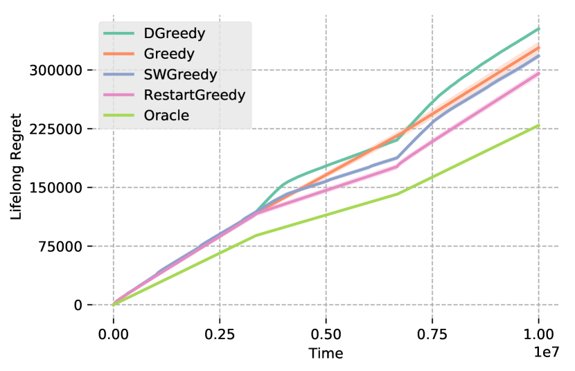
(a) Abruptly changing environment

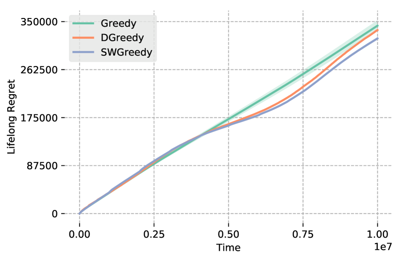
(b) Slowly changing environment

Figure 3: Lifelong regret of various meta-algorithms in non-stationary environments. Shaded areas show standard errors.

In both scenarios, DGreedy and SWGreedy are able to track the change in the prior distribution while the naive Greedy fails to do so. In the abruptly changing scenario, SWGreedy outperforms DGreedy, thus underlining the need to discard data from the previous prior. Regrettably, when the first prior comes back, both algorithms take a long time before finding again the previous learned solution; making the naive Greedy competitive in this experiment even if it completely missed the first change. Conversely in the slowly changing scenario, Greedy fails to track the slow change in the prior distribution and thus accumulates a larger regret with in addition a broad variance. DGreedy and SWGreedy are roughly similar in this case, though SWGreedy performs slightly better in the end. We would also like to mention that there is a hidden parameter in DGreedy. Indeed, in the Greedy algorithm, each arm must have enough information for its index to calculated. In Greedy, and also SWGreedy, this is done by ensuring that each arm has been played at least once. In DGreedy, this initialization is more challenging to determine and we believe it is partly responsible for the poor performance of DGreedy. In both experiments, we arbitrarily set this value to 1.

6 Application to mortal bandits

Finally in this last section, we apply our method to a more realistic setting, the mortal bandit problem [14], where arms appear and disappear regularly (in particular, an arm is not always available contrary to the standard model). While the notion of episode may be more elusive in this setting, we show that synchronizing an episode according to the expected lifetime of arms can help to overcome this difficulty. We look upon the case where this value is known and the one where it is not and thus have to be estimated. We also have to modify the index of the UCB sub-algorithm to take into account that arms arrive at different times and for the unknown expected lifetime. Thereby, we replace the $\log(T)$ term by $\log(t-s_{k}+1)$, where $t$ and $s_{k}$ denotes respectively the current and the arrival time steps for arm $k$. We then again pick the Greedy algorithm as meta-algorithm.

We consider the same setting as [14]. Although they mostly consider a large number of arms, we previously illustrated in Section 3 that this problem can be reduced via sub-sampling to a more tractable one, and with better performance as well. Therefore we focus our attention on problems with a small number of arms. In this setting, the number of arms remains fixed throughout the time horizon $T$, that is when an arm dies, it is immediately replaced by another one. The lifetime of arm $k$, denoted $L_{k}$, is drawn i.i.d. from a Geometric distribution with mean lifetime $L$; this arm died after being available for $L_{k}$ rounds. We also assume that arms are Bernoulli random variables. We consider two scenarios: in the first one, mean rewards of arms are drawn i.i.d. from a uniform distribution over [0, 1], while in the second scenario they are drawn from a Beta(1, 3) distribution. In both cases, we fix the number of arms $K=5$ and the expected lifetime $L=1000$. The horizon is set at $T=1000L$, meaning that there are on average 1000 episodes throughout the time horizon. We compare several algorithms: the untuned UCB algorithm and its optimally tuned variant OracleUCB, along with a tuned AdaptiveGreedy (AG) [14]; and our proposed methods, PeriodicUpdate-UCB (PU-UCB) and EstimatedPeriodicUpdate-UCB (EPU-UCB), where in the first one we assume the knowledge of the expected lifetime, while in the second it is estimated by the empirical mean of dead arms. On top of both our proposed algorithms lie a Greedy algorithm on a discretization of $n=\sqrt{1000}$ points. Results are averaged over 100 runs and are reported on Figure 4.

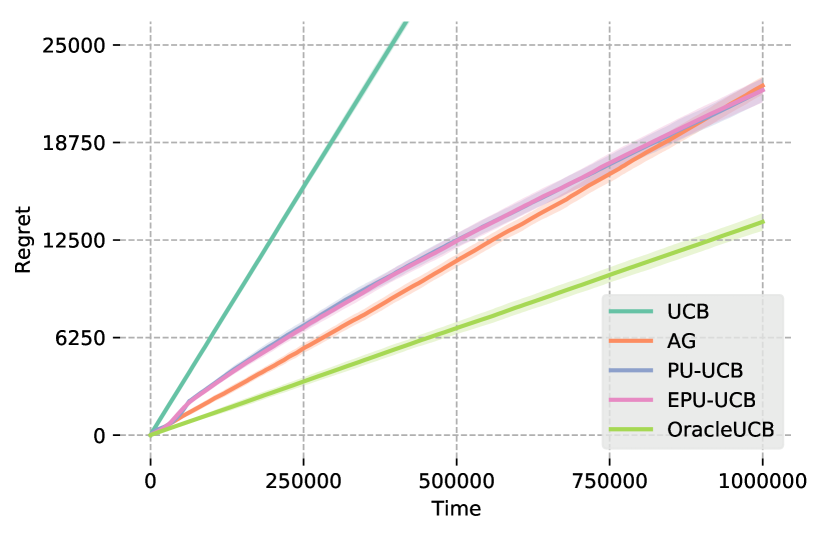
(a) Uniform prior

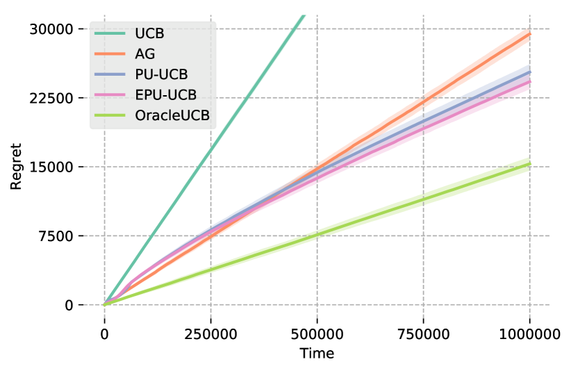
(b) Beta(1, 3) prior

Figure 4: Regret of various algorithms in the mortal bandit setting. Shaded areas show standard errors. PU-UCB and PEU-UCB are almost identical in (a).

These experiments further underline the benefit of tuning the UCB algorithm for practical purposes. AG, a state of the art algorithm in the mortal bandit setting, is clearly outperformed by OracleUCB. Additionally, PU-UCB and EPU-UCB, with somewhat similar performances on both setups, become rapidly better than AG, despite that the latter being optimally tuned. We also remark once more that the regret of both algorithms is sublinear, highlighting the performance of the Greedy meta-algorithm. Interestingly, EPU-UCB performs slightly better than PU-UCB on scenario 2, hinting at a potentially better decomposition of episodes.

7 Conclusion

In this paper, we studied a lifelong learning problem in the multi-armed bandit framework where tasks arrive sequentially, sampled from a problem class with some prior distribution. We first introduced our method which consists in optimize a bandit algorithm, focusing on confidence interval width tuning of UCB-like algorithms. We then considered a bandit over bandit approach employing greedy algorithms as meta-algorithm and evaluated them in both stationary and non-stationary environments. Finally, we applied our method to a more realistic setting, the mortal bandit problem, by decomposing the time horizon into episodes according to the mean lifetime of arms and showed great empirical improvement compared to previous work.

Interesting directions

The most prominent future work, especially in terms of practical applications, concerns the tracking of seasonal environments. It is crucial for building lifelong learning agents. Just recently this problem has been studied in the non-stationary bandit setting [21, 15].

Another direction may be the analysis of the Greedy algorithm in the continuous-armed bandit problem. It has been shown in a recent line a work that it enjoys great performances in several bandit frameworks [5, 27, 6, 40], and this setting is most likely one of them as shown indirectly in our experiments. Although it may be suboptimal, with high probability it concentrates quickly on arms with high expected rewards and thus works extremely well in practice. The next question is the “optimal” discretization for the greatest performance.

Finally in this first work, we focused solely on classical context-free bandits, but extending it to other settings that receive increasing interest, such as contextual [38], combinatorial [19, 39] or multi-player bandits [10, 11], seems also quite crucial and an interesting direction of research.

Appendix A Additional simulations

In this section, we repeat the simulations of Sections 3, 4.1 and 4.2 for different environments.

A.1 Choice of the class of algorithms

In this subsection, we repeat the simulations of Section 3. We recall that we evaluate the Bayesian regret of several UCB-like algorithms as a function of their parameters $\gamma$. We consider two scenarios: the first scenario is a Gaussian bandit problem where mean rewards are drawn i.i.d. from a uniform distribution over $[0,1]$; while the second scenario is a Bernoulli bandit problem where mean rewards are drawn i.i.d. from a Beta(1, 3) distribution. In all experiments, the horizon is fixed at $T=1000$ and we vary the number of arms $K$. Results are averaged over $5000$ iterations and displayed on Figure 5.

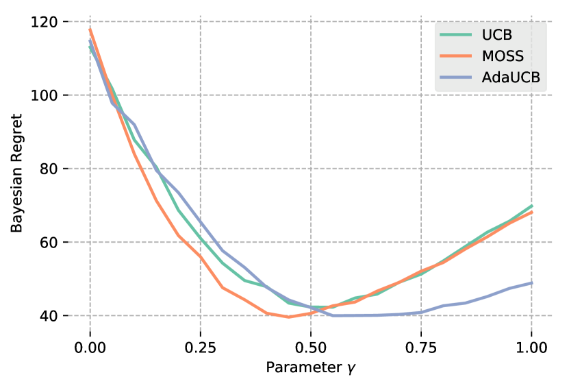
(a) Scenario 1 / $K=5$

(b) Scenario 1 / $K=63$

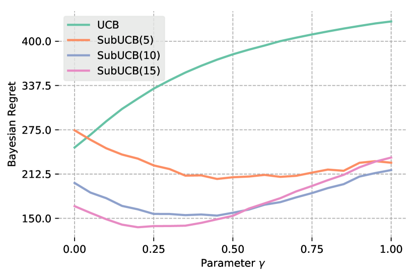
(c) Scenario 1 / $K=250$

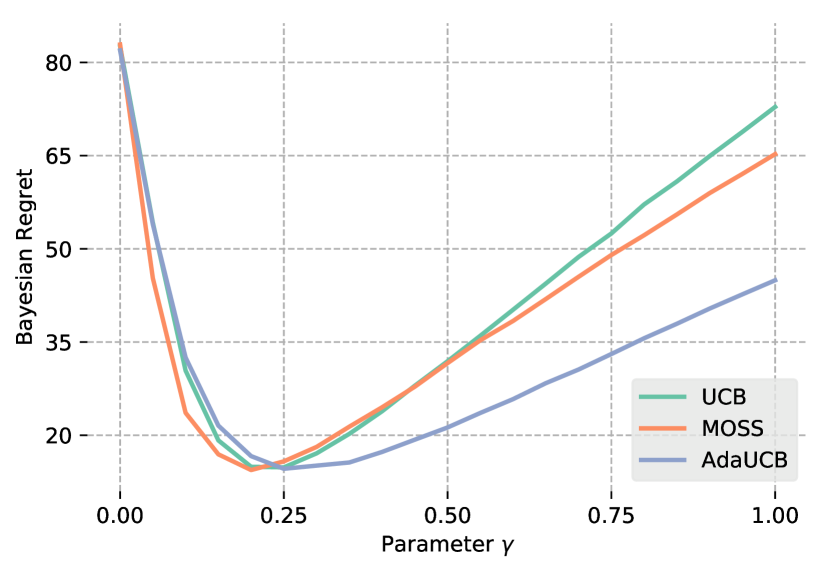
(d) Scenario 2 / $K=5$

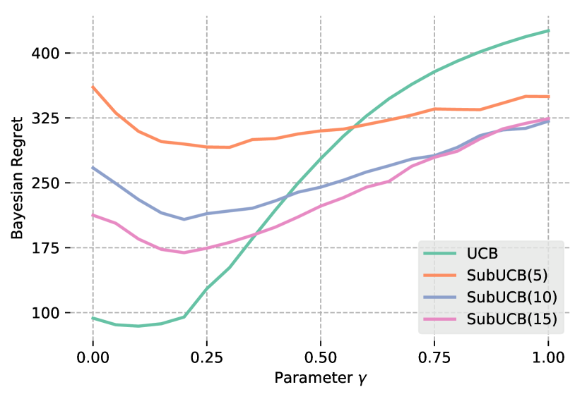
(e) Scenario 2 / $K=63$

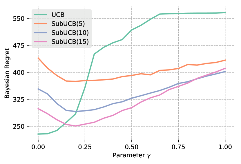
(f) Scenario 2 / $K=250$

Figure 5: Bayesian regret of various algorithms as a function of $\gamma$ for diverse environments and numbers of arms $K$. Rows correspond respectively to Gaussian bandits with a uniform prior and Bernoulli bandits with a Beta(1, 3) prior.

In the first scenario, we observe a similar behavior compared to the Bernoulli case: for small numbers of arms $K$, AdaUCB performs better than UCB for all $\gamma$; for moderate values of $K$, the Greedy algorithm is roughly the best; and for large values $K$, SubUCB performs the best. Similarly, SubUCB($m$) performs better as $m$ grows larger and becomes more sensitive to $\gamma$ at the same time. In the second scenario, the same behavior can be noticed, however what we called moderate and large values of $K$ are, in this case, much higher than previously.

A.2 Influence of the initialization

In this subsection, we repeat the simulations of Section 4.1. We recall that we study the impact of several initializations on the lifelong regret. To do so, we set $\gamma=0.22$ in the UCB algorithm. We consider three scenarios: the first scenario is a Bernoulli bandit problem where mean rewards are drawn i.i.d. from a uniform distribution over $[0,1]$, the second scenario is a Gaussian bandit problem where mean rewards are drawn i.i.d. from a uniform distribution over $[0,1]$ and the third scenario is a Bernoulli bandit problem where mean rewards are drawn i.i.d. from a Beta(1, 3) distribution. In all experiments, the horizon is fixed at $T=1000$ and we vary the number of arms $K$. For $K=5$ and $K=63$, the numbers of episodes is $J=100$, whereas for $K=250$ it is $J=10$. Results are averaged over $500$ iterations for $K=5$, $100$ for the rest, and displayed on Figure 6.

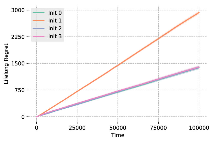
(a) Scenario 1 / $K=5$

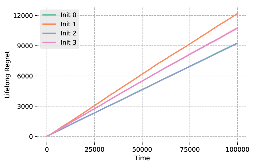
(b) Scenario 1 / $K=63$

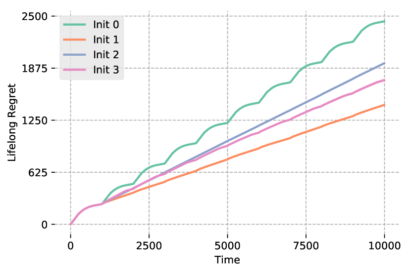
(c) Scenario 1 / $K=250$

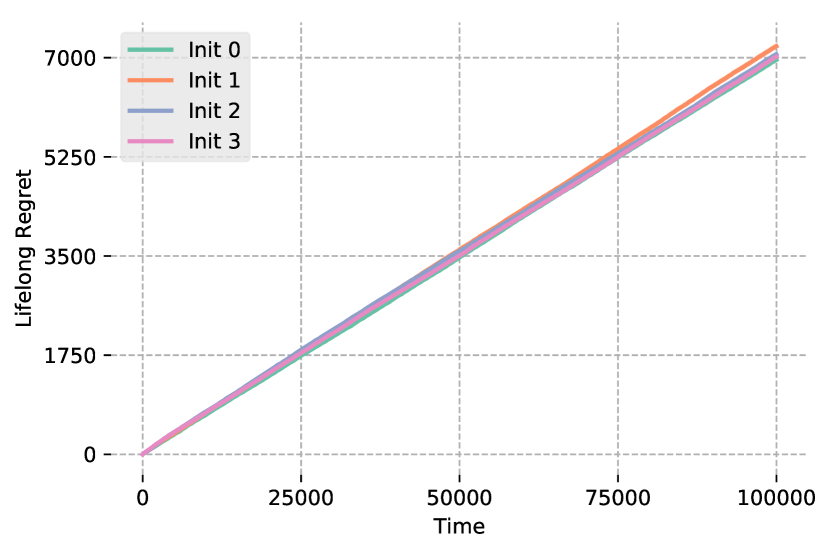
(d) Scenario 2 / $K=5$

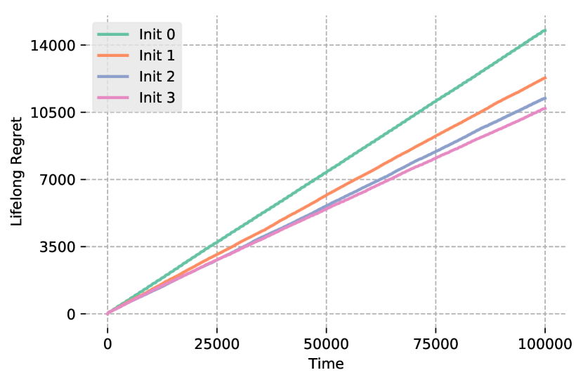
(e) Scenario 2 / $K=63$

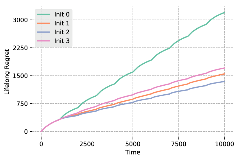
(f) Scenario 2 / K = 250

(g) Scenario 3 / $K=5$

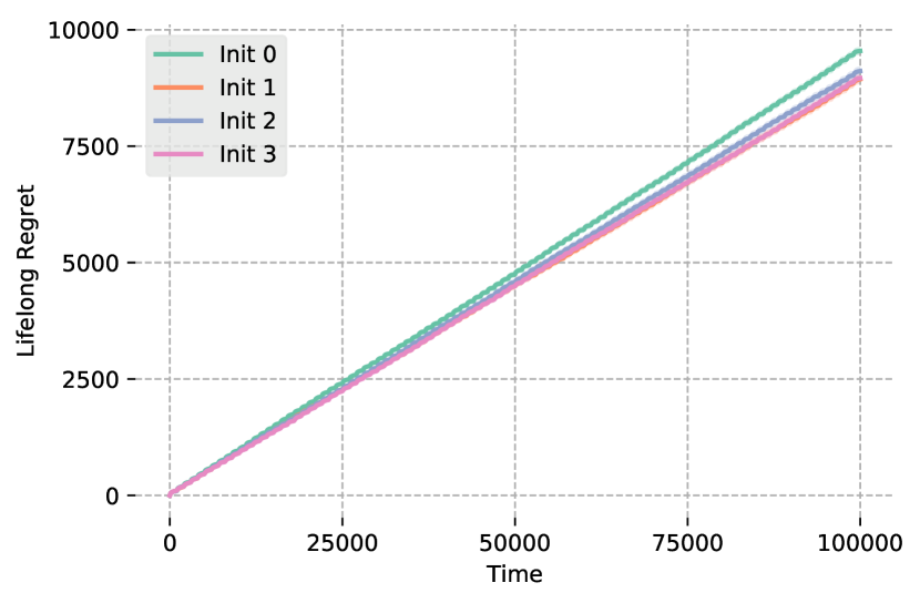
(h) Scenario 3 / $K=63$

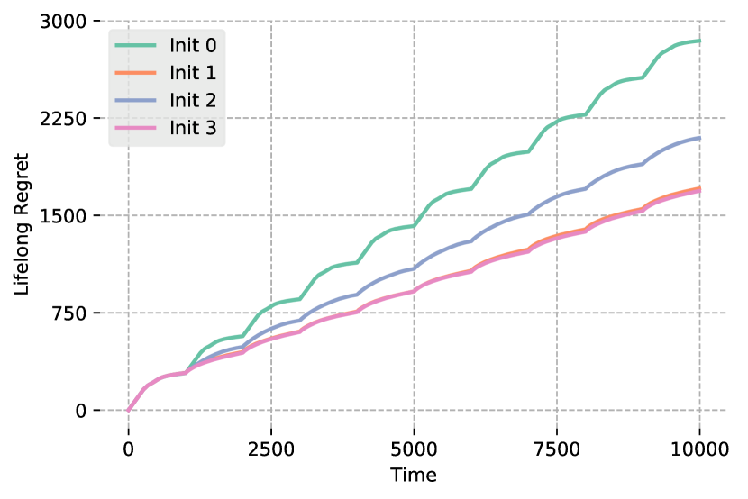
(i) Scenario 3 / $K=250$

Figure 6: Lifelong regret of a deterministic meta-algorithm with various initializations in stationary environments. Rows correspond respectively to Bernoulli bandits with a uniform prior, Gaussian bandits with a uniform prior and Bernoulli bandits with a Beta(1, 3) prior. Shaded areas show standard errors.

It is complex to observe a clear trend across the different simulations. For small values of $K$, the choice of initialization is insignificant; except for the initialization at 0 in the first scenario, they all have roughly the same performance. For intermediate values of $K$, the impact of the choice of initialization becomes apparent. Although there is no optimal choice, initializing arms with the median of previous arms seems more robust. For large value of $K$, a clear trend is emerging: pulling each arm once is always the worst thing to do. It was expected since we spend most of the time initializing arms. There is still no optimal choice in this case, yet the initialization at 0 seems more robust.

A.3 Learning in a stationary environment

In this subsection, we repeat the simulations of Section 4.2. We recall that we study the impact of several meta-algorithms on the lifelong regret. We consider two scenarios: the first scenario is a Gaussian bandit problem where mean rewards are drawn i.i.d. from a uniform distribution over $[0,1]$; while the second scenario is a Bernoulli bandit problem where mean rewards are drawn i.i.d. from a Beta(1, 3) distribution. In all experiments and for each episode, the horizon is fixed at $T=1000$ and the number of arms at $K=5$; and for the meta-algorithm, the number of episodes is set at $J=10000$. Results are averaged over $100$ iterations and illustrated on Figure 7.

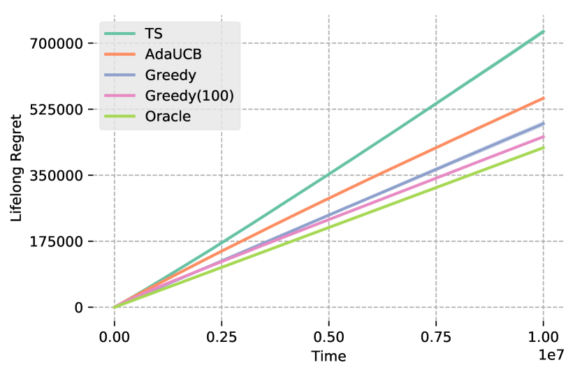
(a) Gaussian bandits with uniform prior

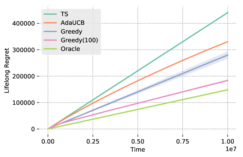
(b) Bernoulli bandits with Beta(1, 3) prior

Figure 7: Lifelong regret of various meta-algorithms in stationary environments. Shaded areas show standard errors.

The results are similar to Section 4.2: TS fails to learn in that time frame, while AdaUCB manages to do so but is outperformed for a long period of time by a naive Greedy. As for Greedy(100), it still performs extremely well; its regret is close to the optimal one and is again sublinear.

References

- [1] Shipra Agrawal and Navin Goyal “Further optimal regret bounds for thompson sampling” In Artificial intelligence and statistics, 2013, pp. 99–107
- [2] Jean-Yves Audibert and Sébastien Bubeck “Minimax policies for adversarial and stochastic bandits”, 2009
- [3] Peter Auer, Nicolo Cesa-Bianchi and Paul Fischer “Finite-time analysis of the multiarmed bandit problem” In Machine learning 47.2-3 Springer, 2002, pp. 235–256
- [4] Peter Auer, Ronald Ortner and Csaba Szepesvári “Improved rates for the stochastic continuum-armed bandit problem” In International Conference on Computational Learning Theory, 2007, pp. 454–468 Springer
- [5] Hamsa Bastani, Mohsen Bayati and Khashayar Khosravi “Mostly exploration-free algorithms for contextual bandits” In arXiv preprint arXiv:1704.09011, 2017
- [6] Mohsen Bayati, Nima Hamidi, Ramesh Johari and Khashayar Khosravi “Optimal and Greedy Algorithms for Multi-Armed Bandits with Many Arms” In arXiv preprint arXiv:2002.10121, 2020
- [7] Donald A Berry and Bert Fristedt “Bandit problems: sequential allocation of experiments (Monographs on statistics and applied probability)” In London: Chapman and Hall 5 Springer, 1985, pp. 71–87
- [8] Zahy Bnaya, Rami Puzis, Roni Stern and Ariel Felner “Volatile multi-armed bandits for guaranteed targeted social crawling” In Workshops at the Twenty-Seventh AAAI Conference on Artificial Intelligence, 2013
- [9] Djallel Bouneffouf and Irina Rish “A survey on practical applications of multi-armed and contextual bandits” In arXiv preprint arXiv:1904.10040, 2019
- [10] Etienne Boursier and Vianney Perchet “SIC-MMAB: synchronisation involves communication in multiplayer multi-armed bandits” In Advances in Neural Information Processing Systems, 2019, pp. 12071–12080
- [11] Etienne Boursier, Emilie Kaufmann, Abbas Mehrabian and Vianney Perchet “A Practical Algorithm for Multiplayer Bandits when Arm Means Vary Among Players” In AISTATS 2020, 2020
- [12] Craig Boutilier et al. “Differentiable Bandit Exploration” In arXiv preprint arXiv:2002.06772, 2020
- [13] Sébastien Bubeck and Nicolo Cesa-Bianchi “Regret analysis of stochastic and nonstochastic multi-armed bandit problems” In arXiv preprint arXiv:1204.5721, 2012
- [14] Deepayan Chakrabarti, Ravi Kumar, Filip Radlinski and Eli Upfal “Mortal multi-armed bandits” In Advances in neural information processing systems, 2009, pp. 273–280
- [15] Ningyuan Chen, Chun Wang and Longlin Wang “Learning and Optimization with Seasonal Patterns” In arXiv preprint arXiv:2005.08088, 2020
- [16] Zhiyuan Chen and Bing Liu “Lifelong machine learning” In Synthesis Lectures on Artificial Intelligence and Machine Learning 10.3 Morgan & Claypool Publishers, 2016, pp. 1–145
- [17] Wang Chi Cheung, David Simchi-Levi and Ruihao Zhu “Hedging the drift: Learning to optimize under non-stationarity” In arXiv preprint arXiv:1903.01461, 2019
- [18] Rémy Degenne and Vianney Perchet “Anytime optimal algorithms in stochastic multi-armed bandits” In Proceedings of The 33rd International Conference on Machine Learning 48, Proceedings of Machine Learning Research New York, New York, USA: PMLR, 2016, pp. 1587–1595 URL: http://proceedings.mlr.press/v48/degenne16.html
- [19] Rémy Degenne and Vianney Perchet “Combinatorial semi-bandit with known covariance” In Advances in Neural Information Processing Systems, 2016, pp. 2972–2980
- [20] Aniket Anand Deshmukh, Urun Dogan and Clay Scott “Multi-task learning for contextual bandits” In Advances in neural information processing systems, 2017, pp. 4848–4856
- [21] Giuseppe Di Benedetto, Vito Bellini and Giovanni Zappella “A Linear Bandit for Seasonal Environments” In arXiv preprint arXiv:2004.13576, 2020
- [22] Aurélien Garivier and Eric Moulines “On upper-confidence bound policies for switching bandit problems” In International Conference on Algorithmic Learning Theory, 2011, pp. 174–188 Springer
- [23] John C Gittins “Bandit processes and dynamic allocation indices” In Journal of the Royal Statistical Society: Series B (Methodological) 41.2 Wiley Online Library, 1979, pp. 148–164
- [24] John Gittins, Kevin Glazebrook and Richard Weber “Multi-armed bandit allocation indices” John Wiley & Sons, 2011
- [25] Cédric Hartland et al. “Multi-armed bandit, dynamic environments and meta-bandits”, 2006
- [26] Chih-Wei Hsu et al. “Empirical bayes regret minimization” In arXiv preprint arXiv:1904.02664, 2019
- [27] Sampath Kannan et al. “A smoothed analysis of the greedy algorithm for the linear contextual bandit problem” In Advances in Neural Information Processing Systems, 2018, pp. 2227–2236
- [28] Emilie Kaufmann “On Bayesian index policies for sequential resource allocation” In arXiv preprint arXiv:1601.01190, 2016
- [29] Robert D Kleinberg “Nearly tight bounds for the continuum-armed bandit problem” In Advances in Neural Information Processing Systems, 2005, pp. 697–704
- [30] Levente Kocsis and Csaba Szepesvári “Bandit based monte-carlo planning” In European conference on machine learning, 2006, pp. 282–293 Springer
- [31] Volodymyr Kuleshov and Doina Precup “Algorithms for multi-armed bandit problems” In arXiv preprint arXiv:1402.6028, 2014
- [32] Tze Leung Lai “Adaptive treatment allocation and the multi-armed bandit problem” In The Annals of Statistics JSTOR, 1987, pp. 1091–1114
- [33] Tor Lattimore “Refining the confidence level for optimistic bandit strategies” In The Journal of Machine Learning Research 19.1 JMLR. org, 2018, pp. 765–796
- [34] Tor Lattimore and Csaba Szepesvári “Bandit algorithms” In preprint, 2018, pp. 28
- [35] Alessandro Lazaric and Emma Brunskill “Sequential transfer in multi-armed bandit with finite set of models” In Advances in Neural Information Processing Systems, 2013, pp. 2220–2228
- [36] Lisha Li et al. “Hyperband: A novel bandit-based approach to hyperparameter optimization” In The Journal of Machine Learning Research 18.1 JMLR. org, 2017, pp. 6765–6816
- [37] Francis Maes, Louis Wehenkel and Damien Ernst “Meta-learning of exploration/exploitation strategies: The multi-armed bandit case” In International Conference on Agents and Artificial Intelligence, 2012, pp. 100–115 Springer
- [38] Vianney Perchet and Philippe Rigollet “The multi-armed bandit problem with covariates” In The Annals of Statistics 41.2 Institute of Mathematical Statistics, 2013, pp. 693–721
- [39] Pierre Perrault, Etienne Boursier, Michal Valko and Vianney Perchet “Statistical efficiency of thompson sampling for combinatorial semi-bandits” In Advances in Neural Information Processing Systems 33, 2020
- [40] Manish Raghavan, Aleksandrs Slivkins, Jennifer Wortman Vaughan and Zhiwei Steven Wu “Greedy Algorithm almost Dominates in Smoothed Contextual Bandits” In arXiv preprint arXiv:2005.10624, 2020
- [41] Daniel Russo and Benjamin Van Roy “Learning to optimize via posterior sampling” In Mathematics of Operations Research 39.4 INFORMS, 2014, pp. 1221–1243
- [42] Jurgen Schmidhuber “Evolutionary principles in self-referential learning” In On learning how to learn: The meta-meta-… hook.) Diploma thesis, Institut f. Informatik, Tech. Univ. Munich 1, 1987, pp. 2
- [43] Daniel L Silver, Qiang Yang and Lianghao Li “Lifelong machine learning systems: Beyond learning algorithms” In 2013 AAAI spring symposium series, 2013
- [44] Aleksandrs Slivkins “Introduction to multi-armed bandits” In arXiv preprint arXiv:1904.07272, 2019
- [45] Sebastian Thrun “Lifelong learning algorithms” In Learning to learn Springer, 1998, pp. 181–209
- [46] Sebastian Thrun and Lorien Pratt “Learning to learn” Springer Science & Business Media, 2012
- [47] Stefano Traca, Cynthia Rudin and Weiyu Yan “Reducing Exploration of Dying Arms in Mortal Bandits” In arXiv preprint arXiv:1907.02571, 2019
- [48] Joannes Vermorel and Mehryar Mohri “Multi-armed bandit algorithms and empirical evaluation” In European conference on machine learning, 2005, pp. 437–448 Springer
- [49] Qingyun Wu, Naveen Iyer and Hongning Wang “Learning contextual bandits in a non-stationary environment” In The 41st International ACM SIGIR Conference on Research & Development in Information Retrieval, 2018, pp. 495–504
- [50] Qingyun Wu, Huazheng Wang, Yanen Li and Hongning Wang “Dynamic Ensemble of Contextual Bandits to Satisfy Users’ Changing Interests” In The World Wide Web Conference, 2019, pp. 2080–2090