Enumeration of planar constellations with an alternating boundary

Abstract

A planar hypermap with a boundary is defined as a planar map with a boundary, endowed with a proper bicoloring of the inner faces. The boundary is said alternating if the colors of the incident inner faces alternate along its contour. In this paper we consider the problem of counting planar hypermaps with an alternating boundary, according to the perimeter and to the degree distribution of inner faces of each color. The problem is translated into a functional equation with a catalytic variable determining the corresponding generating function.

In the case of constellations—hypermaps whose all inner faces of a given color have degree $m\geqslant 2$, and whose all other inner faces have a degree multiple of $m$—we completely solve the functional equation, and show that the generating function is algebraic and admits an explicit rational parametrization.

We finally specialize to the case of Eulerian triangulations—hypermaps whose all inner faces have degree $3$—and compute asymptotics which are needed in another work by the second author, to prove the convergence of rescaled planar Eulerian triangulations to the Brownian map.

1 Introduction

Context and motivations.

The enumerative theory of planar maps has been an active topic in combinatorics since its inception by Tutte in the sixties [28]. A recent account of its developments may be found in the review by Schaeffer [26]. Many such developments were motivated by connections with other fields: theoretical physics, algebraic and enumerative geometry, computer science, probability theory… In this paper, we consider a specific question of map enumeration which finds its origin in the work [14] of the second author on the scaling limit of random planar Eulerian triangulations. In fact, we establish key asymptotic estimates which are needed in the proof that these maps converge to the Brownian map.

Eulerian triangulations are part of a more general family of maps which, following [5], we call hypermaps. These are maps whose faces are bicolored (say, in black and white) in such a way that no two faces of the same color are adjacent. They correspond through duality to bipartite maps. A fairly general enumeration problem consists in counting planar hypermaps with a given degree distribution of faces of each color. This problem is intimately connected [9] with the Ising model on random maps, first solved by Kazakov and Boulatov [23, 6]. It received a lot of attention in the physics literature, due to its rich critical behavior and its connection with the so-called two-matrix model [20]. A nice account of the enumerative results coming from this approach may be found in the last chapter of the book by Eynard [21]. Let us also mention the many recent papers [3, 17, 18, 27] devoted to the local limits of the Ising model on random maps.

To enumerate maps, the standard approach [28] consists in studying the effect of the removal of an edge. Nowadays, this operation is often called “peeling” [19]. In order to turn the peeling into equations, one needs to keep track of one or more auxiliary parameters, called catalytic variables [7], and typically corresponding to boundary lengths. In the context of hypermaps, a further complication occurs, since one needs to keep track of boundary conditions: colloquially speaking, these encode the colors of the faces incident to the boundary. The most tractable boundary condition is the so-called Dobrushin boundary condition, which consists in having the boundary made of two parts: one part will be incident to white faces, and the other to black faces. The Dobrushin boundary condition has the key property that it is invariant under peeling, provided that we always peel an edge at the white-black interface. The resulting equations are solved in [21, 17], see also [4] for a probabilistic interpretation in the context of site percolation. Knowing how to treat Dobrushin boundary conditions, one may then consider “mixed” boundary conditions [21], where there is a prescribed number of white-black interfaces. However, this approach seems to become intractable when the number of interfaces gets large. Here, we are considering the extreme situation where the number of interfaces is maximal, that is to say when white and black faces alternate along the boundary. We call this situation the alternating boundary condition. It arises when considering the layer decomposition of Eulerian triangulations [14]. The alternating boundary condition is not invariant under peeling, but can be made so by adding a monochromatic boundary part, and peeling at the first alternating edge. Through this method, we obtain a functional equation amenable to the kernel method [25, 7]. We do not attempt to solve this equation in general, but we concentrate on the specific case of constellations (encompassing Eulerian triangulations). Thanks to a shortcut, we directly obtain a rational parametrization of the generating function of constellations with an alternating boundary, and having this parametrization at hand is very convenient to compute asymptotics.

Before presenting our results in more detail, let us mention that there exists several bijective approaches to the enumeration of hypermaps [9, 10, 11, 12, 5, 2], but we have not succeeded so far in adapting them to the case of alternating boundary conditions. We leave this as an open problem.

Main results.

Recall that a planar map is a connected multigraph drawn on the sphere without edge crossings, and considered up to continuous deformation. It consists of vertices, edges, faces, and corners. A boundary is a distinguished face, which we often choose as the infinite face when drawing the map on the plane. It is assumed to be rooted, that is to say there is a distinguished corner along the boundary. The other faces are called inner faces.

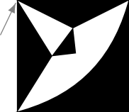
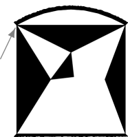
Figure 1: Left: a hypermap with a white monochromatic boundary ($w=\mathord{\circ\circ}\mathord{\circ\circ}$), with its root corner marked by a gray arrow. Right: a hypermap with an alternating boundary ($w=\mathord{\circ\bullet}\mathord{\circ\bullet}$). We paint in black the external sides of the boundary edges with $w_{i}=\bullet$, since the boundary is considered black at these edges.

A hypermap with a boundary is a planar map with a boundary, where every inner face is colored either black or white, in a such a way that adjacent inner faces have different colors. Note that the boundary does not have a specified color: it may be incident to faces of both colors. Let $w$ be a word on the alphabet $\{\bullet,\circ\}$, and $\ell$ be the length of $w$. A hypermap with boundary condition $w$ is a hypermap with a boundary of length $\ell$ such that, when walking in clockwise direction around the map (starting at the root corner),

1. if the $i$-th edge that we visit ($i=1,\ldots,\ell$) is incident to an inner face, then this face is white if $w_{i}=\bullet$ and black if $w_{i}=\circ$,

2. if an edge is incident to the boundary on both sides, and is then visited twice, say at steps $i$ and $j$, then $w_{i}\neq w_{j}$.

In other words, $w_{i}$ codes for the color of the boundary face as seen from the $i$-th edge. A hypermap with a white (resp. black) monochromatic boundary is a hypermap with boundary condition $\circ\circ\cdots\circ$ (resp. $\bullet\bullet\cdots\bullet$). These are just hypermaps in the sense of [5]. A hypermap with an alternating boundary is a hypermap with boundary condition $\circ\bullet\circ\bullet\cdots\circ\bullet$. See Figure 1 for an illustration.

Let $m$ be an integer not smaller than $2$. A hypermap (with a boundary) is called an $m$-constellation if every black (inner) face has degree $m$, and every white (inner) face has degree multiple of $m$. The enumeration of $m$-constellations with a monochromatic boundary and a prescribed degree distribution for the white faces has been considered in previous works [8, 1], and we review the results in Section 2. Our main result concerns the enumeration of $m$-constellations with an alternating boundary:

Theorem 1.

Given a nonnegative integer $r$, let $A_{r}$ denote the generating function of $m$-constellations with an alternating boundary of length $2r$, counted with a weight $t$ per vertex and a weight $x_{i}$ per white inner face of degree $mi$ for every $i\geqslant 1$. By convention, we have $A_{0}=t$, corresponding to the vertex-map. Let $d$ be a positive integer and assume that $x_{i}=0$ for $i>d$. Then, the series

$$A(w):=\sum_{r\geqslant 0}A_{r}w^{r+1}$$ (1)

is algebraic and admits a rational parametrization: for $s$ a formal variable we have

$$A(w(s))=1-\frac{(1+\sum_{k=1}^{d}\alpha_{k}s^{k})^{m-1}}{1+Vs},\qquad w(s):=s\frac{(1+\sum_{k=1}^{d}\alpha_{k}s^{k})^{m-2}}{(1+Vs)^{2}}$$ (2)

where $V$ is the series in $t,x_{1},\ldots,x_{d}$ such that

$$V=t+\sum_{i=1}^{d}\binom{mi-1}{i}x_{i}V^{(m-1)i}$$ (3)

and

$$\alpha_{k}:=\sum_{i=k}^{d}\binom{mi-1}{i-k}x_{i}V^{(m-1)i+k-1},\qquad k=1,\ldots,d.$$ (4)

Note that $w(s)$ is a series in $s$ whose coefficients are polynomials in $V,\alpha_{1},\ldots,\alpha_{d}$, with $w(s)=s+O(s^{2})$. Therefore, the substitution $A(w(s))$ is well-defined and, by reversion of series, we see that $A_{r}$ is a polynomial in $V,\alpha_{1},\ldots,\alpha_{d}$, hence in $V,x_{1},\ldots,x_{d}$. In particular we have $A_{0}=V-(m-1)\alpha_{1}=t$ as wanted. We give the expression for $A_{1}$ in Appendix A, and we also check that it is consistent with the generating function of rooted $m$-constellations computed by another approach. In principle, we may express $A_{r}$ via the Lagrange inversion formula, but we do not expect to obtain a practical formula in this way. Still, as we shall see below, the rational parametrization contains all the information needed to compute asymptotics.

In the case $m=2$, through a classical identification between $2$-constellations and planar bipartite maps, $A_{r}$ should be the generating function of planar bipartite maps with a boundary of length $2r$. This is indeed the case, as we will see in Remark 3 below.

We now focus on the case of Eulerian $m$-angulations (with a boundary), i.e. $m$-constellations whose white (inner) faces all have degree $m$. By specializing Theorem 1 to $d=1$ and $x_{1}=1$, we obtain:

Corollary 1.

For (planar) Eulerian $m$-angulations with an alternating boundary, counted with a weight $t$ per vertex, the rational parametrization takes the form

$$A(w(s))=1-\frac{(1+V^{m-1}s)^{m-1}}{1+Vs},\qquad w(s):=s\frac{(1+V^{m-1}s)^{m-2}}{(1+Vs)^{2}}$$ (5)

where $V$ is the series in $t$ such that $V=t+(m-1)V^{m-1}$.

From this we may compute the first few terms of $A(w)$, namely

$$A(w)=tw+\left(V^{2}+(2m-3)V^{m}+\frac{(m-1)(m-2)}{2}V^{2m-2}\right)w^{2}+\\ \textstyle\left(2V^{3}+(6m-10)V^{m+1}+(m-2)(4m-5)V^{2m-1}-\frac{(m-1)(m-2)(2m-3)}{3}V^{3m-3}\right)w^{3}+\cdots,$$ (6)

and the coefficient of $w^{r}$ is a polynomial in $V$. Note that we may apply again Lagrange inversion, this time on the variable $t$, to get that $V^{k}=\sum_{n\geqslant 0}\frac{k(m-1)^{n}}{mn+k}\binom{mn+k}{n}t^{(m-1)n+k}$ for any $k\geqslant 1$. Plugging this into (6) allows to extract the coefficient of $t^{n}w^{r}$ in $A(w)$.

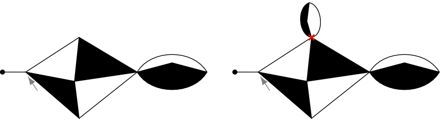
Figure 2: Left: an Eulerian triangulation with a semi-simple alternating boundary. Right: an Eulerian triangulation with an alternating, but not semi-simple boundary: the vertex that violates the semi-simplicity condition is indicated with a red cross.

Let us emphasize that the above results concern maps whose boundary is not necessarily simple. It is however not difficult to deduce a rational parametrization for maps with a simple boundary via a substitution argument. In fact, the layer decomposition introduced in [14] involves Eulerian triangulations with a semi-simple alternating boundary: the external face can have separating vertices, but only on every other boundary vertex. More precisely, if we number the boundary corners $0,1,\ldots,2r-1$ in clockwise direction, $0$ being the root corner, then the boundary is said semi-simple if there is no separating vertex incident to an odd-numbered corner. See Figure 2 for an illustration. Note that this definition allows for separating boundary edges, but such edges are necessarily “pendant”, i.e. incident to a vertex of degree one. From the case $m=3$ of Corollary 1 and through substitution and singularity analysis, we obtain the following results, needed in [14]:

Theorem 2.

For $n,p$ nonnegative integers, denote by $B_{n,p}$ the number of Eulerian triangulations with a semi-simple alternating boundary of length $2p$ and with $n$ black triangles. Then, the corresponding generating function reads

$$B(t,z):=\sum_{n\geqslant 0}\sum_{p\geqslant 0}B_{n,p}t^{n}z^{p}=\frac{1}{16t}\left(8t+8z+\left(1-\sqrt{1-8t}-4z\right)\textstyle\sqrt{\frac{(1+\sqrt{1-8t})^{2}-4z}{1-z}}\right).$$ (7)

For fixed $z\in[0,\frac{1}{4})$, we have the asymptotics

$$[t^{n}]B(t,z)=\sum_{p\geqslant 0}B_{n,p}z^{p}\underset{n\to\infty}{\sim}\frac{3}{2}\frac{z}{\sqrt{\pi(z-1)(4z-1)^{3}}}8^{n}n^{-5/2}$$ (8)

and, for any fixed $p$,

$$B_{n,p}\underset{n\to\infty}{\sim}C(p)8^{n}n^{-5/2},$$ (9)

with

$$C(p)\underset{p\to\infty}{\sim}\frac{\sqrt{3}}{2\pi}4^{p}\sqrt{p}.$$ (10)

Moreover, the quantity $Z(p):=\sum_{n}B_{n,p}8^{-n}=B\left(1/8,z\right)$ is finite for all $p\geqslant 0$, and satisfies

$$\sum_{p\geqslant 0}Z(p)z^{p} =\frac{1}{2}\left(1+8z+\frac{(1-4z)^{3/2}}{(1-z)^{1/2}}\right),$$ (11)

$$Z(p) \underset{p\to\infty}{\sim}\frac{1}{4}\sqrt{\frac{3}{\pi}}4^{p}p^{-5/2},\qquad Z(0)=1.$$ (12)

Note that $B(0,z)=\frac{1}{1-z}$, i.e. $B_{0,p}=1$ for all $p\geqslant 0$: this corresponds to the “star” formed by $p$ edges, the root corner being incident to the central vertex.

The quantity $Z(p)$ can be understood as the partition function of the probability measure on all Eulerian triangulations of the disk having a semi-simple alternating boundary of length $2p$, that assigns a weight $8^{-n}/Z(p)$ to each such triangulation that has $n$ black triangles. In particular, a random Eulerian triangulation sampled according to this law has a fixed perimeter, but not a fixed size, and the variance of that size is infinite. By analogy with similar families of random maps, we therefore call $Z(p)$ the partition function of critical Boltzmann Eulerian triangulations with a semi-simple alternating boundary of length $2p$.

Outline.

In Section 2, we review enumerative results about $m$-constellations with a monochromatic boundary. In Section 3, we derive a functional equation determining the generating function of hypermaps with an alternating boundary of prescribed length. We explain in Section 4 how to solve this equation in the case of $m$-constellations, which leads to the proof of Theorem 1. We consider Eulerian triangulations with a semi-simple alternating boundary in Section 5, and establish Theorem 2. Concluding remarks are gathered in Section 6.

Auxiliary material is left in the appendices: in Appendix A we compute the generating function of rooted $m$-constellations via two approaches; Appendix B deals with the rational parametrization of the generating function of hypermaps with a monochromatic boundary of prescribed length.

Acknowledgments.

We thank Marie Albenque and Grégory Miermont for useful discussions. The work of JB is partly supported by the Agence Nationale de la Recherche via the grant ANR-18-CE40-0033 “Dimers”. The work of AC is supported by the ERC Advanced Grant 740943 GeoBrown.

2 Reminders on the enumeration of constellations

In this section we review enumerative results about $m$-constellations with a monochromatic boundary. Note that an $m$-constellation with a white monochromatic boundary is just a rooted constellation in the classical sense, since the boundary is a white face just like the others, except that one of its corners is distinguished.

Proposition 1 ([8, Theorem 3]).

Let $(n_{i})_{i\geqslant 1}$ be a sequence of nonnegative integers such that $0<\sum n_{i}<\infty$. Then, the number of rooted $m$-constellations having $n_{i}$ white faces of degree $mi$ for every $i\geqslant 1$ is equal to

$$\frac{m}{m-1}\cdot\frac{(v+\sum n_{i}-2)!}{v!}\cdot\prod_{i\geqslant 1}\frac{1}{n_{i}!}\binom{mi-1}{i}^{n_{i}}$$ (13)

where $v=\sum(mi-i-1)n_{i}+2$ is the number of vertices.

The above formula is closely related to the series $V$ of (3). Indeed, by the Lagrange inversion formula, or equivalently by the cyclic lemma, we have

$$\left[x_{1}^{n_{1}}\cdots x_{d}^{n_{d}}\right]V=t^{v-1}\frac{(v+\sum n_{i}-2)!}{(v-1)!}\cdot\prod_{i=1}^{d}\frac{1}{n_{i}!}\binom{mi-1}{i}^{n_{i}}$$ (14)

for $v=\sum(mi-i-1)n_{i}+2$. The right-hand side is precisely equal to $\frac{m-1}{m}vt^{v-1}$ times (13), assuming $d$ large enough. Removing the spurious term $t$ in $V$, we may interpret $\frac{m}{m-1}(V-t)$ as the generating function of pointed rooted constellations, with no weight for the marked vertex. See also the discussion in [13, pp. 130-132]. The generating function of rooted constellations may be deduced by integrating with respect to $t$: we perform this computation in Appendix A.

Let us now consider $m$-constellations with a white monochromatic boundary of prescribed length $mp$, and denote by $F_{p}^{\circ}$ the corresponding generating function, with no weight for the boundary. It was shown in [1] that

$$\frac{dF_{p}^{\circ}}{dt}=\binom{mp}{p}V^{(m-1)p}$$ (15)

and, by integrating and performing the change of variable $t\to V$ using (3), we get

$$F_{p}^{\circ}=\binom{mp}{p}\left(\frac{V^{(m-1)p+1}}{(m-1)p+1}-\sum_{i=1}^{d}\frac{i}{p+i}\binom{mi-1}{i}x_{i}V^{(m-1)(p+i)}\right)$$ (16)

which coincides with [1, Proposition 10] up to an hypergeometric identity.

Interestingly, it is possible to collect all the $(F_{p}^{\circ})_{p\geqslant 0}$ into a single grand generating function which admits a rational parametrization. This property holds at the more general level of hypermaps, as we explain in Appendix B by restating the results from [21, Chapter 8] in our present setting. Let us just state here the result for $m$-constellations:

Proposition 2.

Let $X(y)$ be the formal Laurent series in $y^{-1}$ defined by

$$X(y):=\sum_{i=1}^{d}x_{i}y^{mi-1}+\sum_{p=0}^{\infty}\frac{F_{p}^{\circ}}{y^{mp+1}}$$ (17)

and let $x(z)$ and $y(z)$ be the Laurent polynomials

$$x(z):=z+\sum_{k=1}^{d}\alpha_{k}z^{1-mk},\qquad y(z):=\frac{V}{z}+z^{m-1},$$ (18)

where the $\alpha_{k}$ and $V$ are as in Theorem 1. Then, we have

$$X(y(z))=x(z)$$ (19)

which should be understood as a substitution of series in $z$, $y(z)^{-1}$ being a formal power series in $z$ without constant term.

It may be shown [2] that this proposition is equivalent to the general expression (16) for $(F_{p}^{\circ})_{p\geqslant 0}$. Remarkably, the same Laurent polynomials $x(z)$ and $y(z)$ provide a rational parametrization for the generating function of $m$-constellations with a black monochromatic boundary (see again Appendix B for the derivation):

Proposition 3.

Let $F_{p}^{\bullet}$ denote the generating function of $m$-constellations with a black monochromatic boundary of length $mp$, $p\geqslant 1$, with no weight for the boundary. Let $Y(x)$ be the formal Laurent series in $x^{-1}$ defined by

$$Y(x)=x^{m-1}+\sum_{p=0}^{\infty}\frac{F_{p}^{\bullet}}{x^{mp+1}}.$$ (20)

Then, we have

$$Y(x(z))=y(z)$$ (21)

which should be understood as a substitution of series in $z^{-1}$, $x(z)^{-1}$ being a formal power series in $z^{-1}$ without constant term.

3 A functional equation for hypermaps with an alternating boundary

In this section we consider the general setting of hypermaps: our purpose is to establish a functional equation determining, for all $r\geqslant 0$, the generating function $A_{r}$ of hypermaps with an alternating boundary of length $2r$, counted with a weight $t$ per vertex and weight $t_{i}$ (resp. $\tilde{t}_{i}$) per black (resp. white) inner face of degree $i$ for every $i\geqslant 1$.

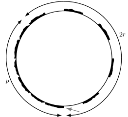
Figure 3: To obtain a functional equation for the enumeration of bicolored maps with an alternating boundary, we consider a more general boundary condition, with a monochromatic part (of length denoted by $p$) and an alternating one (of length denoted by $2r$).

As it is often the case in map enumeration, it is not obvious how to write a recursion determining the family $(A_{r})_{r\geqslant 0}$ directly, but we can obtain a recursion determining the more general family $(M_{p,r})_{p,r\geqslant 0}$, where $M_{p,r}$ is the generating function of hypermaps with “mixed” boundary condition of the form

$$\underbrace{\bullet\bullet\cdots\bullet}_{\text{length }p}\underbrace{\circ\bullet\circ\bullet\cdots\circ\bullet}_{\text{length }2r},$$ (22)

see Figure 3 for an illustration. We then have $A_{r}=M_{0,r}$, while $M_{p,0}$ is equal to the generating function $W_{p}$ of hypermaps with a black monochromatic boundary of length $p$. In view of Theorem 3 in Appendix B below, $W_{p}$ can be considered as known, since (when degrees are bounded) we have a rational parametrization for the grand generating function

$$W(x):=\sum_{p=0}^{\infty}\frac{W_{p}}{x^{p+1}}.$$ (23)

Let us introduce the corresponding generating functions for $A_{r}$ and $M_{p,r}$:

$$A(w):=\sum_{r=0}^{\infty}A_{r}w^{r+1},\qquad M(x,w):=\sum_{p=0}^{\infty}\sum_{r=1}^{\infty}M_{p,r}\frac{w^{r}}{x^{p+1}}.$$ (24)

Our reason for working with series in $x^{-1}$ and $w$, and for shifting some exponents by $1$, is that it will lead to more compact expressions below. Note that, conventionally, $A_{0}=M_{0,0}=W_{0}=t$.

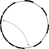
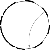
Figure 4: Recursive decomposition of a hypermap with mixed boundary condition, as counted by $M_{p,r}$. We “peel” the first white edge of the alternating part of the boundary, and the three situations illustrated in the top row may occur: we may either discover a new black inner face (left)—which will increase the length of the black monochromatic boundary—or the white edge may be identified to a black edge, either in the monochromatic (middle) or the alternating (right) boundary. The bottom row displays the lengths of the different boundary parts in the second and third cases (we exclude by convention the case $r^{\prime}=r-1$ on the right since it is the same as the case $p^{\prime}=p$ on the left).

Lemma 1.

For $p\geqslant 0$ and $r\geqslant 1$, we have the recursion relation

$$M_{p,r}=\sum_{i\geqslant 1}t_{i}M_{p+i,r-1}+\sum_{p^{\prime}=0}^{p}W_{p^{\prime}}M_{p-p^{\prime},r-1}+\sum_{r^{\prime}=0}^{r-2}A_{r^{\prime}}M_{p,r-r^{\prime}-1}.$$ (25)

Proof.

See Figure 4. ∎

The above recursion translates into the functional equation

$$M(x,w)=w\sum_{i\geqslant 1}t_{i}\left[x^{i}(M(x,w)+W(x))\right]_{x^{<0}}\\ +wxW(x)(M(x,w)+W(x))+A(w)M(x,w)$$ (26)

where the notation $[\cdot]_{x^{<0}}$ means that we keep only terms with negative powers of $x$ (since in the sum over $i$ we “miss” some initial terms of $M(x,w)+W(x)$). We may rewrite the functional equation in the form

$$K(x,w)M(x,w)=R(x,w)$$ (27)

with

$$\begin{split}K(x,w)&:=1-A(w)-wxY(x)\\ R(x,w)&:=wxW(x)Y(x)-w\sum_{i\geqslant 1}t_{i}\left[x^{i}(M(x,w)+W(x))\right]_{x^{\geqslant 0}}\end{split}$$ (28)

where the notation $[\cdot]_{x^{\geqslant 0}}$ should be self-explanatory and

$$Y(x):=\sum_{i\geqslant 1}t_{i}x^{i-1}+W(x)$$ (29)

is the same as in Theorem 3.

We recognize a functional equation in one catalytic variable $x$, which is linear in $M(x,w)$ and thus amenable to the kernel method. When the $t_{i}$ vanish for $i$ large enough, we may rewrite the equation in a form which allows to apply [7, Theorem 3] and conclude that $M(x,w)$, hence $A(w)$, is algebraic in $w$, $x$, $W(x)$ and the $t_{i}$. We will however not attempt to work out an explicit expression for $A(w)$ in general, but we will rather concentrate on the case of $m$-constellations for which there is a simplification, and which is sufficient for the application we have in mind.

4 Simplification in the case of $m$-constellations

We now specialize the face weights to

$$t_{i}=\begin{cases}1&\text{if $i=m$,}\\ 0&\text{otherwise,}\end{cases}\qquad\tilde{t}_{i}=\begin{cases}x_{i/m}&\text{if $m$ divides $i$,}\\ 0&\text{otherwise.}\end{cases}$$ (30)

A simplification occurs due to the following:

Lemma 2.

In the case of constellations, we have $M_{p,r}=0$ unless $m$ divides $p$.

Proof.

A hypermap with a boundary can be endowed with a canonical orientation of it edges, by orienting each edge in order to have, say, white on its right (using the boundary condition for the boundary edges). Assume that the hypermap is an $m$-constellation, and consider a cycle, not necessarily oriented: we denote by $a$ (resp. $b$) the number of clockwise-oriented (resp. counterclockwise-oriented) edges along it. We claim that $m$ divides $a-b$, which may be checked by induction on the number of faces encircled by the cycle. Applying this property to the contour of the boundary (or rather, of each of its simple components), the result follows. ∎

The above lemma implies that

$$M(x,w)+W(x)=\frac{A(w)}{wx}+O\left(\frac{1}{x^{m+1}}\right)$$ (31)

which allows to rewrite the quantity $R(x,w)$ of (28) as

$$R(x,w)=wxW(x)Y(x)-x^{m-1}A(w)=wxY(x)^{2}-wx^{m}Y(x)-x^{m-1}A(w).$$ (32)

We now apply the kernel method, or rather a slight variant as we explain in Remark 2 below. We claim that there exists a unique formal power series $\omega(x)$ in $x^{-1}$ without constant term such that

$$K(x,\omega(x))=0.$$ (33)

Indeed, this condition can be rewritten

$$\omega(x)=\frac{1-A(\omega(x))}{xY(x)}=x^{-m}\frac{1-A(\omega(x))}{1+x^{1-m}W(x)}$$ (34)

which fixes inductively all the coefficients of $\omega(x)$, that turns out to be a series in $x^{-m}$. Then, by (27) and since the substitution $M(x,\omega(x))$ is well-defined, we deduce that

$$R(x,\omega(x))=0.$$ (35)

This gives a linear system of two equations determining $\omega(x)$ and $A(\omega(x))$ as

$$\omega(x)=\frac{x^{m-2}}{Y(x)^{2}},\qquad A(\omega(x))=1-\frac{x^{m-1}}{Y(x)}.$$ (36)

At this stage, we assume that there exists $d$ such that $x_{i}=0$ for $i>d$ (note that we have not used this assumption so far). This allows to plug in the rational parametrization of $Y(x)$ given by Proposition 3. We find

$$\omega(x(z))=\frac{x(z)^{m-2}}{y(z)^{2}},\qquad A(\omega(x(z)))=1-\frac{x(z)^{m-1}}{y(z)}$$ (37)

with $x(z)$ and $y(z)$ given by (18). We now observe that both right-hand sides are actually series in $s=z^{-m}$ and, setting $w(s)=\omega(x(z))$, we obtain the rational parametrization announced in Theorem 1, which is thereby established. We conclude this section by some remarks.

Remark 1.

Even though we assume that there is a bound on faces degrees in Theorem 1, we may take formally the limit $d\to\infty$: by reversion we find that $A_{r}$ is a polynomial in $V,\alpha_{1},\ldots,\alpha_{r+1}$, and each of these quantities is a well-defined series in $t,x_{1},x_{2},\ldots$.

Remark 2.

In the usual kernel method, one would rather look for series $\xi(w)$ such that $K(\xi(w),w)=0$. This would certain succeed but at the price of some complications, since we would find $m$ different Puiseux series in $w^{1/m}$, namely the roots of the equation $\omega(\xi(w))=w$. The reason why our variant works is that $K$ and $R$ involve only one unknown series $A(w)$. This property seems specific to the case of $m$-constellations: indeed, the simplification hinges upon the relation (31), which would fail if we allowed for faces of degree not divisible by $m$, and upon the fact that the sum over $i$ in (28) involves only a single nonzero term for $i=m$, which would not be the case if we allowed for black faces of degree higher than $m$.

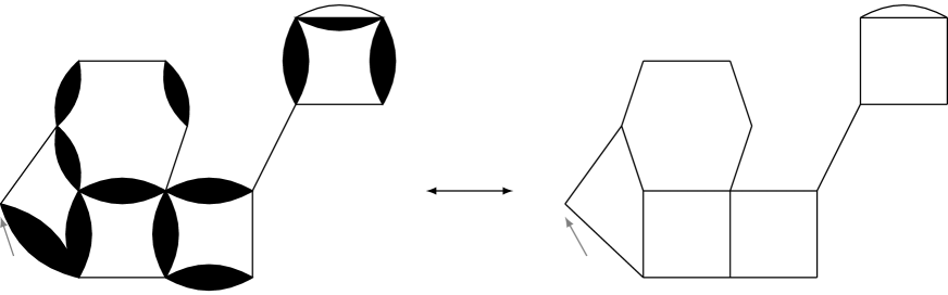
Figure 5: Bijection between 2-constellations with an alternating boundary and bipartite planar maps with a boundary.

Remark 3.

Considering the case $m=2$ provides a nontrivial consistency check. Indeed, as displayed on Figure 5, $2$-constellations with an alternating boundary may be identified with bipartite planar maps with a boundary, whose enumeration is well-known. The rational parametrization (37) takes the form

$$A\left(\frac{1}{y(z)^{2}}\right)=1-\frac{x(z)}{y(z)}.$$ (38)

To match this expression with known formulas, we shall consider the modified generating function $\tilde{A}(y)=\sum_{r\geqslant 0}\frac{A_{r}}{y^{2r+1}}=yA\left(\frac{1}{y^{2}}\right)$. It then admits the rational parametrization

$$\tilde{A}(y(z))=y(z)-x(z)=\frac{V}{z}-\sum_{k\geqslant 1}\frac{\alpha_{k}}{z^{2k-1}}$$ (39)

which matches that given in [21, Theorem 3.1.3], up to the change of variable $z\to\gamma z$, $V=\gamma^{2}$.

Remark 4.

Taking $x=x_{1}$ and $w=\omega(x_{2})$ in (27), and using (32) and (36), we find that the generating function $M(x,w)$ of $m$-constellations with a mixed boundary condition (22) takes the parametric form

$$M(x_{1},\omega(x_{2}))=\frac{1}{x_{1}}\left(\frac{(x_{1}/x_{2})^{m}-1}{x_{1}Y(x_{1})-x_{2}Y(x_{2})}(x_{2}Y(x_{2}))^{2}+x_{1}^{m}-x_{1}Y(x_{1})-x_{2}Y(x_{2})\right)$$ (40)

and a rational parametrization follows by further substituting $x_{1}=x(z_{1})$ and $x_{2}=x(z_{2})$.

5 Asymptotics for Eulerian triangulations

The purpose of this section is to establish Theorem 2. Let us denote by $T_{n,r}$ the number of Eulerian triangulations with a (non necessarily semi-simple) alternating boundary of length $2r$ having $n$ black triangles. We form the generating function

$$T(t,u):=\sum_{n\geqslant 0}\sum_{r\geqslant 0}T_{n,r}t^{n}u^{r}.$$ (41)

In the series $A$ of Theorem 1, we rather attach a weight $t$ to vertices. But, in a triangulation counted by $T_{n,r}$, the number of vertices $v$ is given by

$$v=n+r+1$$ (42)

(observe that there are $n$ white triangles and $3n+r$ edges, then apply Euler’s relation). Thus, the series $A$ specialized to the case of Eulerian triangulations satisfies

$$A(w)=twT(t,tw)$$ (43)

and it follows from the case $m=3$ of Corollary 1, upon taking $w=w(W/V)$ with $W$ a new variable, that $T$ admits the rational parametrization

$$T\left(V-2V^{2},\frac{W(1-2V)(1+VW)}{(1+W)^{2}}\right)=\frac{(1+W)(1-2V-V^{2}W)}{(1-2V)(1+VW)}.$$ (44)

Let us now make the connection with the generating function $B(t,z)$ of Eulerian triangulations with a semi-simple alternating boundary, as defined in Theorem 2. Considering that a triangulation with a general boundary can be decomposed into a semi-simple “core” (which is the semi-simple component containing the root) and general components attached to every other vertex on the boundary, we obtain the substitution relation

$$T(t,u)=B(t,uT(t,u)).$$ (45)

Combining with (44), we obtain that $B(t,z)$ admits the rational parametrization

$$B\left(V-2V^{2},\frac{W(1-2V-V^{2}W)}{1+W}\right)=\frac{(1+W)(1-2V-V^{2}W)}{(1-2V)(1+VW)}.$$ (46)

By eliminating $V$ and $W$, we find that $B(t,z)$ must be a root of the algebraic equation:

$$16t^{3}(z-1)^{2}B^{4}-32t^{2}(z-1)^{2}(t+z)B^{3}\\ +t(z-1)(24t^{2}z+32tz^{2}+16z^{3}-16t^{2}-52tz-16z^{2}-z)B^{2}\\ -z(z-1)(8t^{2}-20t-1)(t+z)B+z^{2}(t+1)^{3}=0.$$ (47)

By solving this quartic equation and picking the unique solution which is a formal power series in $t$ (the others being Laurent series with negative order), we obtain the expression (7) for $B(t,z)$. The first few terms read

$$B(t,z)=\left(1+z+z^{2}+z^{3}+z^{4}+z^{5}+\cdots\right)+t\left(z+2z^{2}+3z^{3}+4z^{4}+5z^{5}+\cdots\right)\\ +t^{2}\left(3z+8z^{2}+15z^{3}+24z^{4}+35z^{5}+\cdots\right)+t^{3}\left(12z+38z^{2}+83z^{3}+152z^{4}+250z^{5}+\cdots\right)\\ +t^{4}\left(56z+199z^{2}+486z^{3}+988z^{4}+1790z^{5}+\cdots\right)+\\ +t^{5}\left(288z+1112z^{2}+2958z^{3}+6536z^{4}+12822z^{5}+\cdots\right)+\cdots.$$ (48)

The asymptotics are then deduced by standard methods of analytic combinatorics. For fixed $z\in(0,1/4)$, the dominant singularity of $B(t,z)$ is at $t=1/8$ with

$$B(t,z)-c_{0}(z)-c_{1}(z)t\sim\frac{2z}{\sqrt{(z-1)(4z-1)^{3}}}(1-8t)^{3/2},\qquad t\to\frac{1}{8}$$ (49)

for some functions $c_{0}(z)$ and $c_{1}(z)$. We then use the transfer theorem [22, Corollary VI.1] to obtain (8), which immediately yields (9). Then, as the function of $z$ appearing in (8) is algebraic and has a unique dominant singularity at $z=1/4$, we can apply the transfer theorem once again to get (10). The asymptotics (11) for $Z(p)$ are obtained by a similar reasoning. All these computations may be checked using the companion Maple file available on the web page of the second author, and the proof of Theorem 2 is now complete.

6 Conclusion

In this paper, we have shown how to enumerate hypermaps with an alternating boundary, explicited the solution in the case of $m$-constellations, and obtained explicit and asymptotic results in the case of Eulerian triangulations with a semi-simple alternating boundary, crucial in the analysis of the layer decomposition of Eulerian triangulations [14].

Our approach relies on the framework of functional equations with catalytic variables arising from the recursive “peeling” decomposition of maps. This framework is closely related to the so-called topological recursion for maps: in a nutshell, the core idea is that, given a family of maps defined by some “bulk” conditions (degree-dependent weights, etc), the corresponding generating functions for all sorts of topologies and boundary conditions can be constructed as functions defined on a common algebraic curve known as the “spectral curve”. In the context of hypermaps (or equivalently the Ising model on maps), this idea is discussed in [21, Chapter 8], and the spectral curve is nothing but the algebraic curve $(x(z),y(z))_{z\in\mathbb{C}\cup\{\infty\}}$ of genus zero that we have been using in this paper. Our results show that alternating boundaries fit nicely in this context, at least in the case of $m$-constellations, since we see from (37) that our series $A(w)$ “lives” on the same spectral curve.

Let us now list some possible directions for future research. First, we have explicited the solution of the functional equation of Section 3 only in the case of $m$-constellations: it might be instructive to treat other cases, such as the Ising model on four-regular maps, which would correspond to taking $t_{2}=\tilde{t}_{2}$ and $t_{4}=\tilde{t}_{4}$ nonzero, and all others $t_{i}$ and $\tilde{t}_{i}$ zero.

Second, one may of course study other types of boundary conditions for hypermaps. In fact, it is widely believed that, in order to understand the metric properties of random maps decorated with an Ising model, one should be able to handle general—or at least “typical”—boundary conditions. Besides this ambitious research program, some specific cases are of interest. As discussed in [15, Chapters 8 and 9], considering alternating boundaries with defects is relevant to the study of metric balls in the Upper Half-Plane Eulerian Triangulation, and our approach extends nicely to this setting. In another direction, if one tries to extend the layer decomposition to, say, Eulerian quadrangulations, then one is led to consider boundary conditions which are obtained by repeating two possible patterns, namely $\circ\bullet$ and $\mathord{\circ\circ}\mathord{\bullet\bullet}$. Handling these generalized alternating boundaries represents a new technical challenge, as one should embed them in a family of peeling-invariant boundary conditions extending (22).

Finally, as mentioned in the introduction, and in view of the quite simple rational parametrization of Corollary 1, it is natural to ask whether our results could be derived by a bijective approach.

Appendix A The generating function of rooted $m$-constellations

Let $C$ denote the generating function of rooted $m$-constellations (i.e., $m$-constellations with a white monochromatic boundary of arbitrary length), counted with a weight $t$ per vertex and a weight $x_{i}$ per white face of degree $mi$ for every $i\geqslant 1$ (including the boundary face). As discussed in Section 2, we have

$$C=\frac{m}{m-1}\int(V-t)dt.$$ (50)

Here and in the following, there are no integration constants since $[t^{0}]C=0$. On the other hand, recalling the definition of $A_{1}$ in Theorem 1, we have

$$C=A_{1}-t^{2},$$ (51)

since there is an obvious bijection between rooted $m$-constellations and $m$-constellations with boundary condition $\bullet\circ$ not reduced to a single edge. From the rational parametrization, we find that

$$A_{1}=V^{2}-(2m-3)V\alpha_{1}+\frac{m-1}{2}\left((m-2)\alpha_{1}^{2}-2\alpha_{2}\right).$$ (52)

Using

$$t=V-(m-1)\alpha_{1},$$ (53)

we deduce that

$$C=\frac{m\alpha_{1}}{2}\left(2V-(m-1)\alpha_{1}\right)-(m-1)(V\alpha_{1}+\alpha_{2}).$$ (54)

Let us check the consistency of this expression with (50). For this, we write

$$\int Vdt=\int VdV-(m-1)\int Vd\alpha_{1}$$ (55)

and hence

$$\begin{split}\frac{m}{m-1}\int(V-t)dt&=\frac{m}{2(m-1)}(V^{2}-t^{2})-m\int Vd\alpha_{1}\\ &=\frac{m}{2}\alpha_{1}\left(2V-(m-1)\alpha_{1}\right)-m\int Vd\alpha_{1}.\end{split}$$ (56)

Thus, comparing with (54), we should have

$$m\int Vd\alpha_{1}=(m-1)(V\alpha_{1}+\alpha_{2}).$$ (57)

This is easy to check using the definition (4) of the $\alpha_{k}$, performing the integration term by term and doing simple manipulations of binomial coefficients.

Remark 5.

The expression (54) is “canonical” as $V,\alpha_{1},\ldots,\alpha_{d}$ are algebraically independent. Indeed, the formal variables $t,x_{1},\ldots,x_{d}$ are by definition independent and they can be recovered polynomially from $V,\alpha_{1},\ldots,\alpha_{d}$.

Appendix B Rational parametrizations for monochromatic boundaries

Hypermaps and the Ising model.

We consider generating functions of hypermaps, counted with a weight $t$ per vertex and a weight $t_{i}$ (resp. $\tilde{t}_{i}$) per black (resp. white) inner face of degree $i$ for every $i=2,\ldots,d$ (resp. $i=2,\ldots,\tilde{d}$), where $d$ and $\tilde{d}$ are fixed integers larger than $1$. In order to stick with the setting of [21], inner faces of degree one are forbidden, but there would be no problem allowing them.

We denote by $W_{p}$ (resp. $\tilde{W}_{p}$) the generating function of hypermaps with a black (resp. white) monochromatic boundary of length $p$, $p\geqslant 0$. We have conventionally $W_{0}=\tilde{W}_{0}=t$.

Theorem 3 (reformulation of [21, Theorem 8.3.1]).

Let $Y(x)$ and $X(y)$ be the formal Laurent series in $x^{-1}$ and $y^{-1}$, respectively, defined by

$$Y(x):=\sum_{i=2}^{d}t_{i}x^{i-1}+\sum_{p=0}^{\infty}\frac{W_{p}}{x^{p+1}},\qquad X(y):=\sum_{i=2}^{\tilde{d}}\tilde{t}_{i}y^{i-1}+\sum_{p=0}^{\infty}\frac{\tilde{W}_{p}}{y^{p+1}}$$ (58)

and let $x(z)$ and $y(z)$ be the Laurent polynomials

$$x(z):=z+\sum_{k=0}^{\tilde{d}-1}a_{k}z^{-k},\qquad y(z):=\frac{V}{z}+\sum_{k=0}^{d-1}b_{k}z^{k}$$ (59)

where $V,a_{0},\ldots,a_{\tilde{d}-1},b_{0},\ldots,b_{d-1}$ are the series in $t,t_{2},\ldots,t_{d},\tilde{t}_{2},\ldots,\tilde{t}_{\tilde{d}}$ determined by the conditions

$$y(z)-\sum_{i=2}^{d}t_{i}x(z)^{i-1}=tz^{-1}+O(z^{-2}),\qquad x(z)-\sum_{i=2}^{\tilde{d}}\tilde{t}_{i}y(z)^{i-1}=\frac{tz}{V}+O(z^{2}).$$ (60)

Then, we have

$$X(y(z))=x(z),\qquad Y(x(z))=y(z)$$ (61)

which should be understood as substitutions of series in $z$ and $z^{-1}$ respectively, $y(z)^{-1}$ (resp. $x(z)^{-1}$) being a formal power series in $z$ (resp. $z^{-1}$) without constant term.

Since we have reformulated slightly the statement given in [21], let us explain the connection. Eynard does not quite consider hypermaps, but rather planar maps whose faces have degree at least $3$ and carry Ising ($+$ or $-$) spins, and where each edge receives a weight $c_{++}$ (resp. $c_{--}$, $c_{+-}$) if it is incident to two $+$ faces (resp. two $-$ faces, one $+$ and one $-$ face). There is a standard one-to-many correspondence between such maps and hypermaps, obtained by “collapsing” the bivalent (degree $2$) faces of the hypermaps and attaching a spin $+$ (resp. $-$) to the remaining black (resp. white) faces. In this correspondence, two adjacent $+$ faces were necessarily separated by an odd number of bivalent faces, with one more white than black bivalent face. Thus, the effective weight per $++$ edge is

$$c_{++}=\frac{\tilde{t}_{2}}{1-t_{2}\tilde{t}_{2}}.$$ (62)

Similarly, for the $--$ and $+-$ edges we get effective weights

$$c_{--}=\frac{t_{2}}{1-t_{2}\tilde{t}_{2}},\qquad c_{+-}=\frac{1}{1-t_{2}\tilde{t}_{2}}.$$ (63)

All these relations can be put in matrix form

$$\begin{pmatrix}c_{++}&c_{+-}\\ c_{+-}&c_{--}\end{pmatrix}=\begin{pmatrix}-t_{2}&1\\ 1&-\tilde{t}_{2}\end{pmatrix}^{-1}$$ (64)

and we get the following identification with the notations from [21, Theorem 8.1.1] (which deals with yet another reformulation of hypermaps):

$$c=-1,\qquad a=-t_{2},\qquad b=-\tilde{t}_{2}.$$ (65)

Plugging into [21, Theorem 8.3.1], $Y(x)$ matches our present definition (58), and we obtain the form (59) for $x(z)$ and $y(z)$ through the change of variable $z\to z/\gamma$, with $\gamma^{2}=V$. The relation $X(y(z))=x(z)$ is obtained by exchanging the roles of white and black faces, and reparametrizing $z\to V/z$.

Remark 6.

Theorem 3 can be given a combinatorial interpretation, as will be explained in [2].

Specialization to constellations.

Let us change the $d$ and $\tilde{d}$ of Theorem 3 into $m$ and $md$, respectively, and set the face weights to

$$t_{i}=\begin{cases}1&\text{if $i=m$,}\\ 0&\text{otherwise,}\end{cases}\qquad\tilde{t}_{i}=\begin{cases}x_{i/m}&\text{if $m$ divides $i$,}\\ 0&\text{otherwise.}\end{cases}$$ (66)

It is not difficult to check that, with such weights, the conditions (60) imply that the series $a_{k}$ and $b_{k}$ vanish unless $m$ divides $k+1$. Thus, $x(z)$ and $y(z)$ can be put in the form (18), the first condition (60) implying that $b_{m-1}=1$. By extracting the coefficient of $z^{1-km}$ for $k\geqslant 1$ in the second condition (60), we find that $\alpha_{k}=a_{mk-1}$ is given by (4), while extracting the coefficient of $z$ yields an equation equivalent to (3). Identifying $F^{\circ}_{p}=\tilde{W}_{mp}$ and $F^{\bullet}_{p}=W_{mp}$, we obtain Propositions 2 and 3 as specializations of Theorem 3.

References

- [1] M. Albenque and J. Bouttier. Constellations and multicontinued fractions: application to Eulerian triangulations. In 24th International Conference on Formal Power Series and Algebraic Combinatorics (FPSAC 2012), Discrete Math. Theor. Comput. Sci. Proc., AR, pages 805–816, 2012.
- [2] M. Albenque and J. Bouttier. On the slice decomposition of planar hypermaps. In preparation, 2021.
- [3] M. Albenque, L. Ménard, and G. Schaeffer. Local convergence of large random triangulations coupled with an Ising model. Trans. Am. Math. Soc., 374(1):175–217, 2021.
- [4] O. Angel. Growth and percolation on the uniform infinite planar triangulation. Geom. Funct. Anal., 13:935–974, 2003.
- [5] O. Bernardi and É. Fusy. Unified bijections for planar hypermaps with general cycle-length constraints. Ann. Inst. Henri Poincaré D, 7(1):75–164, 2020.
- [6] D. V. Boulatov and V. A. Kazakov. The Ising model on a random planar lattice: the structure of the phase transition and the exact critical exponents. Phys. Lett. B, 186(3-4):379–384, 1987.
- [7] M. Bousquet-Mélou and A. Jehanne. Polynomial equations with one catalytic variable, algebraic series and map enumeration. J. Combin. Theory Ser. B, 96(5):623–672, 2006.
- [8] M. Bousquet-Mélou and G. Schaeffer. Enumeration of planar constellations. Adv. in Appl. Math., 24(4):337–368, 2000.
- [9] M. Bousquet-Mélou and G. Schaeffer. The degree distribution in bipartite planar maps: applications to the Ising model. arXiv:math/0211070, 2002.
- [10] J. Bouttier, P. Di Francesco, and E. Guitter. Planar maps as labeled mobiles. Electr. J. Combin., 11(1), 2004.
- [11] J. Bouttier, P. Di Francesco, and E. Guitter. Blocked edges on Eulerian maps and mobiles: application to spanning trees, hard particles and the Ising model. J. Phys. A, 40(27):7411–7440, 2007.
- [12] J. Bouttier, É. Fusy, and E. Guitter. On the two-point function of general planar maps and hypermaps. Ann. Inst. Henri Poincaré Comb. Phys. Interact., 1:265–306, 2014.
- [13] J. Bouttier. Physique statistique des surfaces aléatoires et combinatoire bijective des cartes planaires. Doctoral thesis, Université Pierre et Marie Curie – Paris 6, June 2005. https://tel.archives-ouvertes.fr/tel-00010651.
- [14] A. Carrance. Convergence of Eulerian triangulations. arXiv:1912.13434, 2019.
- [15] A. Carrance. Random colored triangulations. Doctoral thesis, Université de Lyon, September 2019. https://tel.archives-ouvertes.fr/tel-02338972.
- [16] G. Chapuy and M. Dołęga. Non-orientable branched coverings, -Hurwitz numbers, and positivity for multiparametric Jack expansions. arXiv:2004.07824, 2020.
- [17] L. Chen and J. Turunen. Critical Ising model on random triangulations of the disk: enumeration and local limits. Commun. Math. Phys., 374(3):1577–1643, 2020.
- [18] L. Chen and J. Turunen. Ising model on random triangulations of the disk: phase transition. arXiv:2003.09343, 2020.
- [19] N. Curien. Peeling random planar maps. Lecture notes of the 2019 Saint-Flour Probability Summer School, preliminary version available at https://www.math.u-psud.fr/~curien/enseignement.html, 2019.
- [20] M. R. Douglas. The two-matrix model. In Random surfaces and quantum gravity (Cargèse, 1990), volume 262 of NATO Adv. Sci. Inst. Ser. B Phys., pages 77–83. Plenum, New York, 1991.
- [21] B. Eynard. Counting surfaces, volume 70 of Progress in Mathematical Physics. Birkhäuser/Springer, [Cham], 2016. CRM Aisenstadt chair lectures.
- [22] P. Flajolet and R. Sedgewick. Analytic combinatorics. Cambridge University Press, Cambridge, 2009.
- [23] V. A. Kazakov. Ising model on a dynamical planar random lattice: exact solution. Phys. Lett. A, 119(3):140–144, 1986.
- [24] S. Lando and A. Zvonkin. Graphs on surfaces and their applications, volume 141 of Encyclopaedia of Mathematical Sciences. Springer-Verlag, Berlin, 2004. With an appendix by Don B. Zagier, Low-Dimensional Topology, II.
- [25] H. Prodinger. The kernel method: a collection of examples. Sém. Lothar. Combin., B50f, 19, 2004.
- [26] G. Schaeffer. Planar maps. In Handbook of enumerative combinatorics, Discrete Math. Appl. (Boca Raton), pages 335–395. CRC Press, Boca Raton, FL, 2015.
- [27] J. Turunen. Interfaces in the vertex-decorated Ising model on random triangulations of the disk. arXiv:2003.11012, 2020.
- [28] W. T. Tutte. On the enumeration of planar maps. Bull. Amer. Math. Soc., 74:64–74, 1968.