Training Signal Design for Sparse Channel Estimation in Intelligent Reflecting Surface-Assisted Millimeter-Wave Communication

Abstract

In this paper, the problem of training signal design for intelligent reflecting surface (IRS)-assisted millimeter-wave (mmWave) communication under a sparse channel model is considered. The problem is approached based on the Cram$\acute{\text{e}}$r-Rao lower bound (CRB) on the mean-square error (MSE) of channel estimation. By exploiting the sparse structure of mmWave channels, the CRB for the channel parameter composed of path gains and path angles is derived in closed form under Bayesian and hybrid parameter assumptions. Based on the derivation and analysis, an IRS reflection pattern design method is proposed by minimizing the CRB as a function of design variables under constant modulus constraint on reflection coefficients. Numerical results validate the effectiveness of the proposed design method for sparse mmWave channel estimation.

I Introduction

IRSs have gained much attention as one of the potential technologies for 6G under various names such as reconfigurable intelligent surfaces (RISs), reflector-arrays or intelligent walls. The objective of communication system design up to now was to design optimal signal waveforms and encoding/decoding schemes for given wireless channels, but IRSs have changed the paradigm of this conventional communication system design. IRSs aim to realize intelligent wireless channels by controlling the radio propagation model rather than optimizing transmission-and-reception schemes under given channels [1, 2]. An IRS consists of an array of passive scattering elements and the phase and/or other characteristics of the signal reflected by each element is controlled. The controllable radio propagation model is beneficial for wireless communication to improve signal quality and coverage [5], [6], and various aspects of the IRS technology have been investigated. The propagation and pathloss model with IRS was studied [3] and the design of transmit beamformer and IRS phase shifters was examined with various objectives and constraints. For example, the problem of sum rate maximization under a transmit power constraint was studied in [4] and the maximization of minimum signal-to-interference-plus-noise ratio (SINR) subject to a given power constraint was considered in [5]. The transmit power and phase shift of IRS were optimized to improve energy efficiency in downlink multiuser MISO channels with IRS in [6]. The secrecy rate performance associated with IRS was investigated in [7, 8, 9, 10]. Simultaneous wireless information and power transfer (SWIPT) was also considered in the context of IRS in [11]. In particular, IRSs can be very useful in mmWave channels since the propagation is directive and the propagation loss is large in this band. IRSs can provide diversity paths to improve the link quality to fully harness the large bandwidth available in this band [12, 13]. In this regard, the authors in [14] designed a transmit precoder and the IRS reflection pattern for data transmission in mmWave channels. For such design of transmit beamformer and IRS phase shifters, channel state information (CSI) is required and most previous works assume that perfect CSI of the IRS and the direct link is available. However, in practice, channels should be estimated. Channel estimation in IRS-assisted communication is not simple because an IRS is composed of passive reflecting elements which cannot send their own pilot signal and this fact makes the available channel estimation methods devised for relay channels not directly applicable. In this paper, we consider mmWave communication, which can potentially get much benefit from IRSs, and investigate training signal design for channel estimation in IRS-assisted mmWave communication.

I-A Related Works and Contributions

We here focus on works on channel estimation in IRS-assisted communication relevant to our work. One line of approaches to channel estimation in IRS-assisted systems is to estimate individual channels, i.e., one from the transmitter to the IRS and the other from the IRS to the receiver [15, 16]. Under the assumption that the channel between the base station and the IRS varies slowly as compared to the channel between the IRS and a user, the authors in [15, 16] proposed two-step channel estimation frameworks. These approaches enable the precoding schemes in [17, 18] to be feasible, which require the knowledge of individual channels. Another approach is to estimate the cascaded channel composed of the transmitter-to-IRS and IRS-to-receiver channels by treating the cascaded channel as a single effective channel [19, 20, 21, 22] (this approach is adopted in this study). In [19], the authors proposed an one-by-one channel estimation protocol in which only a single IRS element is activated while other elements remain off in each step. In [20], the authors investigated a cascaded channel framework, exploiting sparse matrix factorization and matrix completion techniques in a downlink massive multiple-input multiple-output (MIMO) system. Under the assumption of a rank-deficient channel, the pilot symbols and the IRS reflection pattern having on-off states are generated randomly by using Gaussian and Bernoulli distributions, respectively. In [21], the authors designed an optimal channel estimation scheme based on minimization of the Cram$\acute{\text{e}}$r-Rao lower bound (CRB) under a dense channel model and showed that an optimal IRS activation patterns was given by the columns of the discrete Fourier transform (DFT) matrix. In [22], a transmission protocol to perform channel estimation and IRS optimization successively was proposed for an IRS-based orthogonal frequency division multiplexing (OFDM) system.

The majority of the existing works assume that the number of training symbols for channel estimation is large enough as compared to the number of (grouped) IRS reflecting elements [15, 16, 19, 20, 21, 22]. However, it can be difficult to satisfy this assumption in practical systems because an IRS typically adopts a large number of reflecting elements to achieve high passive beamforming gain. The contributions of this paper are summarized as follows.

• We incorporated the channel sparsity in mmWave channels into the signal model to reduce the number of parameters to be estimated. The parameter in this case is given by path gains and path angles, and the considered framework enables channel estimation with the reduced number of pilot symbols less than the number of the reflecting elements in the IRS.

• We derived the CRB under two assumptions: One is that both path gains and path angles are random parameters with known distributions and the other is that the path gains are random but the path angles are deterministic and unknown.

• In the Bayesian parameter case, we derived a condition to minimize the Bayesian CRB and showed that the Fisher information “density” for angle estimation was given by a quadratic form composed of the derivative of the array response and the IRS reflection pattern matrix square and this determined the quality of angle estimation across the angle domain.

• In the hybrid parameter case, treating the path gains as random nuisance parameters, we formulated the problem of optimal IRS reflection pattern matrix design by minimizing the CRB on angle estimation, and solved this optimization problem by using the projected gradient method (PGM) [23, 24].

• With numerical evaluation, we demonstrated that the proposed design method exploiting channel sparsity yielded noticeable gain in sparse mmWave channels when the number of training symbols was less than the number of the reflecting elements in the IRS.

I-B Notations and Organization

Vectors and matrices are written in boldface with matrices in capitals. All vectors are column vectors. For a matrix ${\bf A}$, $\mathbf{A}^{T}$, $\mathbf{A}^{H}$, and $\mathbf{A}^{\dagger}$ indicate the transpose, Hermitian transpose, and Moore-Penrose inverse of $\mathbf{A}$, respectively. ${\bf A}\succeq 0$ means that the matrix ${\bf A}$ is a Hermitian positive semidefinite matrix. $[{\bf A}]_{i,j}$ denotes the $(i,j)$-th element of ${\bf A}$. $[{\bf A}]_{i_{1}:i_{2},j_{1}:j_{2}}$ denotes the submatrix of ${\bf A}$ given by the intersection of rows $i_{1},\ldots,i_{2}$ and columns $j_{1},\ldots,j_{2}$. For a vector ${\bf a}$, $[{\bf a}]_{i}$ denotes the $i$-th element of ${\bf a}$, and $\|{\bf a}\|$ represents vector $\ell_{2}$-norm. $\mathbf{0}_{n}$ and $\mathbf{1}_{n}$ are the zero vector of length $n$ and the vector of length $n$ composed of all one elements, respectively. ${\bf e}_{n}(i)$ denotes the $i$-th column vector of the identity matrix of size $n\times n$. ${\bf I}_{n}$ is the identity matrix of size $n\times n$. $\text{diag}({\bf A})$ denotes a vector of the elements on the diagonal of ${\bf A}$ and $\text{diag}({\bf a})$ denotes a diagonal matrix whose diagonal is ${\bf a}$. ${\mathbb{E}}\{\cdot\}$ denotes statistical expectation. ${\bf a}\sim\mathcal{CN}(\hbox{\boldmath$\mu$\unboldmath},\hbox{$\bf\Sigma$})$ means that random vector ${\bf a}$ is complex circularly-symmetric Gaussian distributed with mean vector $\mu$ and covariance matrix $\bf\Sigma$. ${\bf a}\sim\text{Unif}[a,b]$ means that the elements of ${\bf a}$ are randomly and uniformly distributed over the interval $[a,b]$. ${\mathbb{C}}$ denotes the set of complex numbers. The symbol $\odot$ and $\otimes$ denote the Hadamard product and the Kronecker product, respectively. $\text{Re}(\cdot)$ $\text{Im}(\cdot)$ denote the real part and the imaginary part, respectively. $\text{tr}(\cdot)$ denotes the trace operator. $\text{vec}(\cdot)$ denotes the vectorization to stack the columns of the input matrix. $\iota:=\sqrt{-1}$.

This paper is organized as follows. The system model is described in Section II. In Section III, the IRS reflection pattern design is considered under the Bayesian CRB. In Section IV, the IRS reflection pattern design is considered under the hybrid CRB. Numerical results are provided in Section V, followed by conclusions in Section VI.

II System Model

We consider an IRS system composed of a transmitter, an IRS, and a receiver, as shown in Fig. 1. We assume that the transmitter and the receiver have a single antenna and the IRS has a uniform linear array (ULA) of $N$ passive reflecting elements. We assume that there exists a direct channel path from the transmitter to the receiver, where the direct-path channel gain is denoted by $\alpha_{0}\in{\mathbb{C}}$, and there exist channel links between the transmitter and the IRS ${\bf h}^{(t)}=[h_{1}^{(t)},\cdots,h_{N}^{(t)}]^{T}\in\mathbb{C}^{N}$ and between the IRS and the receiver ${\bf h}^{(r)}=[h_{1}^{(r)},\cdots,h_{N}^{(r)}]^{T}\in\mathbb{C}^{N}$. We assume that the considered IRS system operates in the mmWave band and hence adopt a geometry-based sparse channel model relevant to mmWave communication [25, 26, 14, 13, 27]. Thus, the channel vectors of ${\bf h}^{(t)}$ and ${\bf h}^{(r)}$ are modelled as

$${\bf h}^{(t)}=\sum_{i=1}^{L^{(t)}}\alpha_{i}^{(t)}{\bf u}_{N}(\psi_{i}^{(t)})~{}~{}~{}\mbox{and}~{}~{}~{}{\bf h}^{(r)}=\sum_{j=1}^{L^{(r)}}\alpha_{j}^{(r)}{\bf u}_{N}(\psi_{j}^{(r)}),$$ (1)

where $\alpha_{i}^{(t)}$ and $\psi_{i}^{(t)}$ are the gain and angle-of-departure (AoD) of the $i$-th path of the channel from the transmitter to the IRS, $\alpha_{j}^{(r)}$ and $\psi_{j}^{(r)}$ are the gain and angle-of-arrival (AoA) of the $j$-th path of the channel from the IRS to the receiver, $L^{(t)}$ and $L^{(r)}$ are the numbers of multi-paths of ${\bf h}^{(t)}$ and ${\bf h}^{(r)}$, respectively, and ${\bf u}_{N}(\psi)$ is the array response vector of an $N$-element ULA, given by ${\bf u}_{N}(\psi)=\left[1,e^{\iota\pi\psi},e^{\iota\pi 2\psi},\cdots,e^{\iota\pi(N-1)\psi}\right]^{T}$. Here, $\psi$ is the normalized path angle given by $\psi=\frac{2d\sin(\phi)}{\lambda}$, $d$ is the spacing between adjacent reflecting elements at the IRS, $\lambda$ is the carrier wavelength, and $\phi\in[-\pi/2,\pi/2]$ is the unnormalized physical path angle. We assume critical spatial sampling at the IRS, i.e., $d=\frac{\lambda}{2}$, and hence $\psi\in[-1,1]$.

\psfrag{(tx)}[c]{\small TX}\psfrag{(rx)}[c]{\small RX}\psfrag{(w1)}[c]{\small $w_{1k}$}\psfrag{(w2)}[c]{\small $w_{2k}$}\psfrag{(wN)}[c]{\small$w_{Nk}$}\psfrag{(alpha0)}[c]{\small Direct path $\alpha_{0}$}\psfrag{(ht1)}[c]{\small $h_{1}^{(t)}$}\psfrag{(ht2)}[c]{\small $h_{2}^{(t)}$}\psfrag{(htN)}[c]{\small $h_{N}^{(t)}$}\psfrag{(hr1)}[l]{\small $h_{1}^{(r)}$}\psfrag{(hr2)}[l]{\small $h_{2}^{(r)}$}\psfrag{(hrN)}[l]{\small $h_{N}^{(r)}$}\psfrag{(at1)}[c]{\small $\alpha_{1}^{(t)}{\bf u}_{N}(\psi_{1}^{(t)})$}\psfrag{(at2)}[c]{\small\hskip 14.40007pt $\alpha_{L^{(t)}}^{(t)}{\bf u}_{N}(\psi_{L^{(t)}}^{(t)})$}\psfrag{(ar1)}[c]{\small\hskip 6.29997pt $\alpha_{1}^{(r)}{\bf u}_{N}(\psi_{1}^{(r)})$}\psfrag{(arN)}[c]{\small $\alpha_{L^{(r)}}^{(r)}{\bf u}_{N}(\psi_{L^{(r)}}^{(r)})$}\psfrag{(irs)}[c]{\small IRS (ULA with $N$ reflecting elements)}\psfrag{(hybrid)}[l]{\normalsize${\bf f}_{k}^{(i)}$}\includegraphics[scale={0.8}]{figures/system_model_v1.eps}          \psfrag{(tx)}[c]{\small TX}\psfrag{(rx)}[c]{\small RX}\psfrag{(w1)}[c]{\small $w_{1k}$}\psfrag{(w2)}[c]{\small $w_{2k}$}\psfrag{(wN)}[c]{\small$w_{Nk}$}\psfrag{(alpha0)}[c]{\small Direct path $\alpha_{0}$}\psfrag{(ht1)}[c]{\small $h_{1}^{(t)}$}\psfrag{(ht2)}[c]{\small $h_{2}^{(t)}$}\psfrag{(htN)}[c]{\small $h_{N}^{(t)}$}\psfrag{(hr1)}[l]{\small $h_{1}^{(r)}$}\psfrag{(hr2)}[l]{\small $h_{2}^{(r)}$}\psfrag{(hrN)}[l]{\small $h_{N}^{(r)}$}\psfrag{(at1)}[c]{\small $\alpha_{1}^{(t)}{\bf u}_{N}(\psi_{1}^{(t)})$}\psfrag{(at2)}[c]{\small\hskip 14.40007pt $\alpha_{L^{(t)}}^{(t)}{\bf u}_{N}(\psi_{L^{(t)}}^{(t)})$}\psfrag{(ar1)}[c]{\small\hskip 6.29997pt $\alpha_{1}^{(r)}{\bf u}_{N}(\psi_{1}^{(r)})$}\psfrag{(arN)}[c]{\small $\alpha_{L^{(r)}}^{(r)}{\bf u}_{N}(\psi_{L^{(r)}}^{(r)})$}\psfrag{(irs)}[c]{\small IRS (ULA with $N$ reflecting elements)}\psfrag{(hybrid)}[l]{\normalsize${\bf f}_{k}^{(i)}$}\includegraphics[scale={0.8}]{figures/channel_model_v1.eps} (a) System model (b) Channel model

Figure 1: The considered IRS-assisted point-to-point communication link.

We consider training-based channel estimation with a training period composed of $K$ symbols in the beginning of each channel coherence interval. At the $k$-th symbol time during the training period (i.e., $1\leq k\leq K$), the transmitter sends a training symbol $s_{k}$ with $\mathbb{E}\{|s_{k}|^{2}\}=\rho$, and the $N$ passive reflecting elements at the IRS reflect the incoming signal from the transmitter with a complex gain vector ${\bf w}_{k}=[w_{1k},\ldots,w_{Nk}]^{T}$ with $|w_{nk}|=\sqrt{\beta}$ for some $\beta\in(0,1]$. Then, the received signal $y_{k}$ at the receiver at the $k$-th symbol time is given by [13, 14, 27]

$$y_{k}=\left(\alpha_{0}+\sum_{n=1}^{N}w_{nk}^{*}h^{(t)}_{n}h^{(r)}_{n}\right)s_{k}+n_{k}=\left(\alpha_{0}+{\bf w}_{k}^{H}\left({\bf h}^{(t)}\odot{\bf h}^{(r)}\right)\right)\sqrt{\rho}+n_{k},$$ (2)

where $n_{k}\sim{\cal C}{\cal N}(0,\sigma_{n}^{2})$ is circularly-symmetric complex Gaussian noise. The IRS-assisted cascaded channel vector ${\bf h}$ from the transmitter to the receiver is defined as

$${\bf h} :={\bf h}^{(t)}\odot{\bf h}^{(r)}=\sum_{i=1}^{L^{(t)}}\sum_{j=1}^{L^{(r)}}\alpha_{i}^{(t)}\alpha_{j}^{(r)}{\bf u}_{N}\left(\psi_{i}^{(t)}+\psi_{j}^{(r)}\right)=\sum_{\ell=1}^{L}\alpha_{\ell}{\bf u}_{N}(\psi_{\ell})={\bf U}_{\boldsymbol{\psi}}[\alpha_{1},\cdots,\alpha_{L}]^{T},$$ (3)

where $L=L^{(t)}L^{(r)}$ denotes the number of paths in the cascaded channel ${\bf h}$, $\alpha_{\ell}~{}(=\alpha_{i}^{(t)}\alpha_{j}^{(r)})$ and $\psi_{\ell}~{}(=\psi_{i}^{(t)}+\psi_{j}^{(r)})$ denote the effective gain and angle of the $\ell$-th path of the cascaded channel ${\bf h}$, respectively, and ${\bf U}_{\boldsymbol{\psi}}=[{\bf u}_{N}(\psi_{1}),\cdots,{\bf u}_{N}(\psi_{L})]\in\mathbb{C}^{N\times L}$. Then, based on (2), the received signal during the entire training period can be written in vector form as

$${\bf y} ={\bf S}\underbrace{\left[\begin{array}[]{cc}\mathbf{1}_{K}&{\bf W}^{H}\end{array}\right]}_{=:\widetilde{{\bf W}}^{H}}\left[\begin{array}[]{c}\alpha_{0}\\ {\bf h}\end{array}\right]+{\bf n}={\bf S}\widetilde{{\bf W}}^{H}\left[\begin{array}[]{cc}1&\mathbf{0}_{L}^{T}\\ \mathbf{0}_{N}&{\bf U}_{\boldsymbol{\psi}}\end{array}\right]\boldsymbol{\alpha}+{\bf n},$$ (9)

where ${\bf y}=[y_{1},y_{2},\ldots,y_{K}]^{T}$, ${\bf n}=[n_{1},n_{2},\ldots,n_{K}]^{T}$, ${\bf S}=\mbox{diag}(s_{1},\cdots,s_{K})$, ${\bf W}=[{\bf w}_{1},\cdots,{\bf w}_{K}]\in\mathbb{C}^{N\times K}$, and $\hbox{\boldmath$\alpha$\unboldmath}=[\alpha_{0},\alpha_{1},\ldots,\alpha_{L}]^{T}$. We will refer to ${\bf W}$ as the reflection pattern matrix used at the IRS during the training period.

The goal of channel estimation is to obtain the channel parameters $\alpha$ and $\hbox{\boldmath$\psi$\unboldmath}=[\psi_{1},\cdots,\psi_{L}]^{T}$ based on the received signal ${\bf y}$. Once the channel ${\bf h}$ is estimated during the training period, some control information can be sent from the receiver to the IRS to match the reflection coefficients $\{w_{ij}\}$ to ${\bf h}$ in order to maximize the data rate or other desired performance measure based on the received signal model (2) during the data transmission period.

Remark 1

Due to the existence of the direct path, the signal model (9) incorporating the channel sparsity in the mmWave band has a special structure. It is not a simple linear model in terms of the unknown parameters $\{\alpha_{0},\alpha_{1},\cdots,\alpha_{L},\psi_{1},\cdots,\psi_{L}\}$ or a signal model associated with simple AoA estimation. It is a mixed nonlinear model in terms of the channel path-gain parameters $\alpha_{0},\alpha_{1},\cdots,\alpha_{L}$ and the path-angle parameters $\psi_{1},\cdots,\psi_{L}$.

Remark 2

Note that the IRS is typically equipped a large number $N$ of passive reflecting elements to maximize its reflection power. In this case, the number of parameters to be estimated is potentially large, i.e., ${\bf h}\in\mathbb{C}^{N}$ with large $N$. However, by exploiting the sparse scattering nature of mmWave channels (i.e., the value of $L$ is relatively small), we can reduce the required time for training because of the reduced size of channel parameters $\hbox{\boldmath$\alpha$\unboldmath}\in\mathbb{C}^{L+1}$ and $\hbox{\boldmath$\psi$\unboldmath}\in\mathbb{R}^{L}$.

For the rest of this paper, we consider the problem of optimal training signal design under the signal model (9). Under the signal model (9), we have two design variables ${\bf S}$ and ${\bf W}$, where ${\bf S}=\mbox{diag}(s_{1},\cdots,s_{K})$ is the training symbol sequence at the transmitter and ${\bf W}$ is the IRS reflection pattern matrix during the training period. In the context of IRS, we set $s_{k}=\sqrt{\rho}$, $1\leq k\leq K$, i.e., ${\bf S}=\sqrt{\rho}{\bf I}_{K}$ during the training period for analytical tractability and focus on the design of the IRS reflection pattern matrix ${\bf W}$ in the remainder of this paper. Then, the goal is to design the IRS reflection pattern matrix ${\bf W}$ so that channel estimation based on the designed ${\bf W}$ yields best performance under a reasonable criterion. Among several existing criteria for training signal design [28, 15, 16, 19, 20, 21, 22], we adopt the CRB on the MSE of unbiased channel estimation [29, 21], and optimize the IRS reflection pattern matrix ${\bf W}$ by minimizing the CRB as a function of ${\bf W}$. The CRB for given parameter $\theta$ is expressed as [30]

$${\mathbb{E}}_{\boldsymbol{y}|\boldsymbol{\theta}}\{({\mbox{\boldmath$\theta$\unboldmath}}-\hat{{\mbox{\boldmath$\theta$\unboldmath}}}({\bf y}))({\mbox{\boldmath$\theta$\unboldmath}}-\hat{{\mbox{\boldmath$\theta$\unboldmath}}}({\bf y}))^{H}\}\succeq{\bf J}({\mbox{\boldmath$\theta$\unboldmath}})^{-1},$$ (10)

where $\theta$ is the unknown parameter vector, given by ${\mbox{\boldmath$\theta$\unboldmath}}=[\hbox{\boldmath$\alpha$\unboldmath}^{T},\hbox{\boldmath$\psi$\unboldmath}^{T}]^{T}$ in our case, $\hat{{\mbox{\boldmath$\theta$\unboldmath}}}({\bf y})$ is any unbiased estimator of $\theta$, and ${\bf J}({\mbox{\boldmath$\theta$\unboldmath}})$ is the Fisher information matrix (FIM) given by the covariance matrix of the score function $\frac{\partial}{\partial\boldsymbol{\theta}}\ln p({\bf y}|{\mbox{\boldmath$\theta$\unboldmath}})$, i.e., ${\bf J}({\mbox{\boldmath$\theta$\unboldmath}})={\mathbb{E}}_{\boldsymbol{y}|\boldsymbol{\theta}}\left\{\left(\frac{\partial}{\partial\boldsymbol{\theta}}\ln p({\bf y}|{\mbox{\boldmath$\theta$\unboldmath}})\right)\left(\frac{\partial}{\partial\boldsymbol{\theta}}\ln p({\bf y}|{\mbox{\boldmath$\theta$\unboldmath}})\right)^{H}\right\}$.

III Analysis from Bayesian CRB

The derivation of FIM and corresponding CRB depends on the assumption on the parameter ${\mbox{\boldmath$\theta$\unboldmath}}=[\hbox{\boldmath$\alpha$\unboldmath}^{T},\hbox{\boldmath$\psi$\unboldmath}^{T}]^{T}$. In this section, to gain insights into the IRS reflection pattern matrix design with analytical tractability in the sparse channel case, we consider the Bayesian approach that assumes a prior distribution on $\theta$ and considers the MSE performance averaged over the prior distribution on $\theta$. The Bayesian CRB is obtained by taking expectation ${\mathbb{E}}_{\boldsymbol{\theta}}$ over $p({\mbox{\boldmath$\theta$\unboldmath}})$ on both sides of (10) as

$${\mathbb{E}}_{\boldsymbol{\theta}}{\mathbb{E}}_{\boldsymbol{y}|\boldsymbol{\theta}}\{({\mbox{\boldmath$\theta$\unboldmath}}-\hat{{\mbox{\boldmath$\theta$\unboldmath}}}({\bf y}))({\mbox{\boldmath$\theta$\unboldmath}}-\hat{{\mbox{\boldmath$\theta$\unboldmath}}}({\bf y}))^{H}\}\stackrel{{\scriptstyle(a)}}{{\succeq}}{\mathbb{E}}_{\boldsymbol{\theta}}\{{\bf J}({\mbox{\boldmath$\theta$\unboldmath}})^{-1}\}\stackrel{{\scriptstyle(b)}}{{\succeq}}\left({\mathbb{E}}_{\boldsymbol{\theta}}\{{\bf J}({\mbox{\boldmath$\theta$\unboldmath}})\}\right)^{-1},$$ (11)

where Step (b) is valid due to Jensen’s inequality on positive-definite matrix inverse. Hence, the inverse of the averaged FIM or Bayesian FIM ${\mathbb{E}}_{\boldsymbol{\theta}}\{{\bf J}({\mbox{\boldmath$\theta$\unboldmath}})\}$ provides a tractable lower bound on the channel estimation MSE averaged over both ${\bf y}$ and $\theta$.

III-A Derivation of Bayesian CRB

In high-frequency channels such as mmWave channels, the gain and angle of a path are typically uncorrelated [31, 32, 33]. Hence, we assume that $\alpha$ and $\psi$ are statistically independent with marginal distributions $p(\hbox{\boldmath$\alpha$\unboldmath})$ and $p(\hbox{\boldmath$\psi$\unboldmath})$, respectively. From the signal model (9) with additive Gaussian noise, the joint probability density function (pdf) is written as

$$p({\bf y},{\mbox{\boldmath$\theta$\unboldmath}})=p({\bf y},\hbox{\boldmath$\alpha$\unboldmath},\hbox{\boldmath$\psi$\unboldmath}) =p({\bf y}|\hbox{\boldmath$\alpha$\unboldmath},\hbox{\boldmath$\psi$\unboldmath})p(\hbox{\boldmath$\alpha$\unboldmath})p(\hbox{\boldmath$\psi$\unboldmath})=\frac{1}{\left(\pi\sigma_{n}^{2}\right)^{K}}\text{exp}\left(-\frac{1}{\sigma_{n}^{2}}\left\|{\bf y}-{\bf m}\right\|^{2}\right)p(\hbox{\boldmath$\alpha$\unboldmath})p(\hbox{\boldmath$\psi$\unboldmath}),$$ (12)

where ${\bf m}:=\sqrt{\rho}\widetilde{{\bf W}}^{H}\left[\alpha_{0},{\bf h}^{T}\right]^{T}$, as seen in (9). Note that $\alpha$ is complex-valued whereas $\psi$ is real-valued. Hence, it is convenient to consider the real-valued version $\tilde{{\mbox{\boldmath$\theta$\unboldmath}}}$ of the parameter vector $\theta$, defined as $\tilde{{\mbox{\boldmath$\theta$\unboldmath}}}:=\left[\text{Re}\{\hbox{\boldmath$\alpha$\unboldmath}^{T}\},\text{Im}\{\hbox{\boldmath$\alpha$\unboldmath}^{T}\},\hbox{\boldmath$\psi$\unboldmath}^{T}\right]^{T}$. By using the property of the mapping ${\bf x}\mapsto\scalebox{0.8}{$\begin{bmatrix}\text{Re}\{\mathbf{x}\}\\ \text{Im}\{\mathbf{x}\}\end{bmatrix}$}$ for a complex vector ${\bf x}$, the Bayesian CRB for the real-valued version of the parameter is given by [29]

$$\mathbb{E}_{{\bf y},\boldsymbol{\theta}}\biggl{\{}\left(\tilde{{\mbox{\boldmath$\theta$\unboldmath}}}-g({\bf y})\right)\left(\tilde{{\mbox{\boldmath$\theta$\unboldmath}}}-g({\bf y})\right)^{H}\biggr{\}}\succeq{\bf J}_{\tilde{\boldsymbol{\theta}}\tilde{\boldsymbol{\theta}}}^{-1},$$ (13)

for any unbiased channel estimator $g({\bf y})$ for $\tilde{{\mbox{\boldmath$\theta$\unboldmath}}}$, where the real-valued version Bayesian FIM ${\bf J}_{\tilde{\boldsymbol{\theta}}\tilde{\boldsymbol{\theta}}}$ is given by [29]

$$\hskip 100.00015pt{\bf J}_{\tilde{\boldsymbol{\theta}}\tilde{\boldsymbol{\theta}}}=\tilde{{\bf M}}\left[\begin{array}[]{ccc}{\bf J}_{\boldsymbol{\alpha}\boldsymbol{\alpha}}&{\bf J}_{\boldsymbol{\alpha}\boldsymbol{\alpha}^{*}}&{\bf J}_{\boldsymbol{\alpha}\boldsymbol{\psi}}\\ {\bf J}_{\boldsymbol{\alpha}^{*}\boldsymbol{\alpha}}&{\bf J}_{\boldsymbol{\alpha}^{*}\boldsymbol{\alpha}^{*}}&{\bf J}_{\boldsymbol{\alpha}^{*}\boldsymbol{\psi}}\\ {\bf J}_{\boldsymbol{\psi}\boldsymbol{\alpha}}&{\bf J}_{\boldsymbol{\psi}\boldsymbol{\alpha}^{*}}&{\bf J}_{\boldsymbol{\psi}\boldsymbol{\psi}}\\ \end{array}\right]\tilde{{\bf M}}^{H},$$ (17)

$$\hskip 40.00006pt\tilde{{\bf M}}=\left[\begin{array}[]{cc}{\bf M}&\mathbf{0}_{2(L+1)}\mathbf{0}_{L}^{T}\\ \mathbf{0}_{L}\mathbf{0}_{2(L+1)}^{T}&{\bf I}_{L}\end{array}\right],~{}~{}~{}~{}~{}~{}{\bf M}=\frac{1}{2}\left[\begin{array}[]{ccc}{\bf I}_{L+1}&{\bf I}_{L+1}\\ -j{\bf I}_{L+1}&j{\bf I}_{L+1}\end{array}\right],$$ (22)

$${\bf J}_{\boldsymbol{\alpha}\boldsymbol{\alpha}} =-\mathbb{E}_{{\bf y},\boldsymbol{\theta}}\left\{\frac{\partial}{\partial\boldsymbol{\alpha}^{*}}\left(\frac{\partial\ln p({\bf y},\boldsymbol{\alpha},\boldsymbol{\psi})}{\partial\boldsymbol{\alpha}^{*}}\right)^{H}\right\},~{}~{}~{}~{}~{}{\bf J}_{\boldsymbol{\alpha}\boldsymbol{\alpha}^{*}}=-\mathbb{E}_{{\bf y},\boldsymbol{\theta}}\left\{\frac{\partial}{\partial{\boldsymbol{\alpha}^{*}}}\left(\frac{\partial\ln p({\bf y},\boldsymbol{\alpha},\boldsymbol{\psi})}{\partial{\boldsymbol{\alpha}}}\right)^{H}\right\},$$ (23)

and ${\bf J}_{\boldsymbol{\alpha}\boldsymbol{\psi}}$, ${\bf J}_{\boldsymbol{\alpha}^{*}\boldsymbol{\psi}}$, ${\bf J}_{\boldsymbol{\psi}\boldsymbol{\alpha}}$, ${\bf J}_{\boldsymbol{\psi}\boldsymbol{\alpha}^{*}}$ and ${\bf J}_{\boldsymbol{\psi}\boldsymbol{\psi}}$ are similarly defined by considering that $\boldsymbol{\psi}$ is a real-valued vector. Here, $\mathbb{E}_{{\bf y},\boldsymbol{\theta}}$ denotes the expectation with respect to the joint pdf $p({\bf y},\boldsymbol{\theta})=p({\bf y},\hbox{\boldmath$\alpha$\unboldmath},\hbox{\boldmath$\psi$\unboldmath})$, ${\bf M}$ in (22) is the complex-to-real conversion matrix [29, 34], and $\frac{\partial}{\partial{\boldsymbol{\alpha}}}$ and $\frac{\partial}{\partial{\boldsymbol{\alpha}^{*}}}$ in (23) are the Wirtinger complex derivative [35]. Note that the Bayesian FIM does not depend on the parameters $\alpha$ and $\psi$, and the parameter subscript in (17) is for matrix partition purpose.

To enable derivation of Bayesian CRB with still incorporating many meaningful distributions [36, 37], we assume that the direct path gain $\alpha_{0}$ has non-zero mean $\mu_{0}$, the reflected path gains $\alpha_{\ell}$, $\ell=1,\cdots,L$ have zero mean, and all the path gains $\alpha_{\ell}$, $\ell=0,1,\cdots,L$ have the same finite second-order central moment $\sigma^{2}$, and that the path angle is uniformly distributed over $[\Delta_{1},\Delta_{2}]\subset[-1,1]$, i.e., $\psi_{\ell}\stackrel{{\scriptstyle i.i.d.}}{{\sim}}\mbox{Unif}[\Delta_{1},\Delta_{2}]$, $\ell=1,\cdots,L$. Under this prior assumption, the Bayesian CRB is given by the following theorem.

Theorem 1

For the system model in (9) with $\mathbb{E}\{\hbox{\boldmath$\alpha$\unboldmath}\}=\hbox{\boldmath$\mu$\unboldmath}=[\mu_{0},\mathbf{0}_{L}^{T}]^{T}$, $\mathbb{E}\{(\hbox{\boldmath$\alpha$\unboldmath}-\hbox{\boldmath$\mu$\unboldmath})(\hbox{\boldmath$\alpha$\unboldmath}-\hbox{\boldmath$\mu$\unboldmath})^{H}\}=\sigma^{2}{\bf I}_{L+1}$, and $\psi_{\ell}\stackrel{{\scriptstyle i.i.d.}}{{\sim}}\mbox{Unif}[\Delta_{1},\Delta_{2}]$, $\ell=1,\cdots,L$, the Bayesian CRB for any unbiased estimator of $\tilde{{\mbox{\boldmath$\theta$\unboldmath}}}$ is given by $\text{tr}\left({\bf J}_{\tilde{\boldsymbol{\theta}}\tilde{\boldsymbol{\theta}}}^{-1}\right)$, where ${\bf J}_{\tilde{\boldsymbol{\theta}}\tilde{\boldsymbol{\theta}}}={\bf J}_{\tilde{\boldsymbol{\theta}}\tilde{\boldsymbol{\theta}},D}+{\bf J}_{\tilde{\boldsymbol{\theta}}\tilde{\boldsymbol{\theta}},P}$. The likelihood part ${\bf J}_{\tilde{\boldsymbol{\theta}}\tilde{\boldsymbol{\theta}},D}$ and the prior part ${\bf J}_{\tilde{\boldsymbol{\theta}}\tilde{\boldsymbol{\theta}},P}$ are given by

$${\bf J}_{\tilde{\boldsymbol{\theta}}\tilde{\boldsymbol{\theta}},D} =\tilde{{\bf M}}\left[\begin{array}[]{cc|c}{\bf J}_{\boldsymbol{\alpha}\boldsymbol{\alpha},D}&\mathbf{0}_{L+1}\mathbf{0}_{L+1}^{T}&\mathbf{0}_{L+1}\mathbf{0}_{L}^{T}\\ \mathbf{0}_{L+1}\mathbf{0}_{L+1}^{T}&{\bf J}_{\boldsymbol{\alpha}\boldsymbol{\alpha},D}^{*}&\mathbf{0}_{L+1}\mathbf{0}_{L}^{T}\\ \hline\cr\mathbf{0}_{L}\mathbf{0}_{L+1}^{T}&\mathbf{0}_{L}\mathbf{0}_{L+1}^{T}&{\bf J}_{\boldsymbol{\psi}\boldsymbol{\psi},D}\\ \end{array}\right]\tilde{{\bf M}}^{H}$$ (27)

$${\bf J}_{\tilde{\boldsymbol{\theta}}\tilde{\boldsymbol{\theta}},P} =\tilde{{\bf M}}\left[\begin{array}[]{cc|c}{\bf J}_{\boldsymbol{\alpha}\boldsymbol{\alpha},P}&\mathbf{0}_{L+1}\mathbf{0}_{L+1}^{T}&\mathbf{0}_{L+1}\mathbf{0}_{L}^{T}\\ \mathbf{0}_{L+1}\mathbf{0}_{L+1}^{T}&{\bf J}_{\boldsymbol{\alpha}^{*}\boldsymbol{\alpha}^{*},P}&\mathbf{0}_{L+1}\mathbf{0}_{L}^{T}\\ \hline\cr\mathbf{0}_{L}\mathbf{0}_{L+1}^{T}&\mathbf{0}_{L}\mathbf{0}_{L+1}^{T}&{\bf J}_{\boldsymbol{\psi}\boldsymbol{\psi},P}\end{array}\right]\tilde{{\bf M}}^{H},$$ (31)

where

$${\bf J}_{\boldsymbol{\alpha}\boldsymbol{\alpha},D} =\frac{\rho}{\sigma_{n}^{2}}\left[\begin{array}[]{cc}K&(\boldsymbol{\varphi}_{\psi}^{H}\bar{{\bf w}})^{*}\mathbf{1}_{L}^{T}\\ (\boldsymbol{\varphi}_{\psi}^{H}\bar{{\bf w}})\mathbf{1}_{L}&\left(\displaystyle\sum_{m=0}^{N-1}\sum_{n=0}^{N-1}\varphi_{\psi}((n-m)\pi)[{\bf Q}]_{m+1,n+1}\right){\bf I}_{L}+\boldsymbol{\varphi}_{\psi}^{H}{\bf Q}\boldsymbol{\varphi}_{\psi}(\mathbf{1}_{L}\mathbf{1}_{L}^{T}-{\bf I}_{L})\end{array}\right],$$ (34)

$${\bf J}_{\boldsymbol{\psi}\boldsymbol{\psi},D} =\frac{2\rho\sigma^{2}}{\sigma_{n}^{2}}\left(\pi^{2}\sum_{m=1}^{N-1}\sum_{n=1}^{N-1}mn\varphi_{\psi}(\pi(n-m))[{\bf Q}]_{m+1,n+1}\right){\bf I}_{L},$$ (35)

$${\bf J}_{\boldsymbol{\alpha}\boldsymbol{\alpha},P} =-\mathbb{E}\left\{\frac{\partial}{\partial\boldsymbol{\alpha}^{*}}\left(\frac{\partial\ln p(\boldsymbol{\theta})}{\partial\boldsymbol{\alpha}^{*}}\right)^{H}\right\},~{}{\bf J}_{\boldsymbol{\alpha}^{*}\boldsymbol{\alpha}^{*},P}=-\mathbb{E}\left\{\frac{\partial}{\partial\boldsymbol{\alpha}}\left(\frac{\partial\ln p(\boldsymbol{\theta})}{\partial\boldsymbol{\alpha}}\right)^{H}\right\},~{}{\bf J}_{\boldsymbol{\psi}\boldsymbol{\psi},P}=\mathbf{0}_{L}\mathbf{0}_{L}^{T},$$ (36)

$$\bar{{\bf w}} =\left[\bar{w}_{1},\ldots,\bar{w}_{N}\right]^{T}=\sum_{k=1}^{K}{\bf w}_{k},~{}~{}~{}~{}~{}{\bf Q}={\bf W}{\bf W}^{H},~{}~{}~{}\mbox{and}$$ (37)

$$\boldsymbol{\varphi}_{\psi} =\left[{\small\begin{array}[]{c}\vspace{-0.5em}1\\ \varphi_{\psi}(\pi)\\ \vspace{-0.5em}\vdots\\ \varphi_{\psi}\left((N-1)\pi\right)\end{array}}\right]~{}~{}~{}\text{with}~{}~{}~{}\varphi_{\psi}(n\pi)=\frac{2e^{\iota n\pi\left(\frac{\Delta_{2}+\Delta_{1}}{2}\right)}}{n\pi(\Delta_{2}-\Delta_{1})}\sin\left(n\pi\left(\frac{\Delta_{2}-\Delta_{1}}{2}\right)\right).$$ (42)

Proof: See Appendix -A.

III-B Analysis with the Least Information Prior Assumption

Solving the optimization problem for the reflection pattern matrix by minimizing the Bayesian CRB in Theorem 1 is not easy in general cases. In this subsection, we consider the least information prior case under the assumption of Theorem 1 and investigate the reflection pattern matrix design in this case. To this end, we assume that the direct path gain is modelled by Rician fading (i.e., $\alpha_{0}\sim\mathcal{CN}(\mu_{0},\sigma^{2})$), the indirect path gain is modelled by Rayleigh fading (i.e., $\alpha_{\ell}\sim{\cal C}{\cal N}(0,\sigma^{2})$ for $\ell=1,\ldots,L$), and the path angle is uniformly distributed over the entire angle domain (i.e., $\psi_{\ell}{\sim}\mbox{Unif}[-1,1]$, $\ell=1,\cdots,L$). These prior distributions of $\alpha_{\ell}$ and $\psi_{\ell}$ have maximum entropy under the finite second moment and finite support assumptions, respectively. Based on this prior assumption, the Bayesian FIM is given by the following corollary.

Corollary 1

For the signal model (9) with $\hbox{\boldmath$\alpha$\unboldmath}\sim\mathcal{CN}(\hbox{\boldmath$\mu$\unboldmath},\sigma^{2}{\bf I}_{L+1})$, $\hbox{\boldmath$\mu$\unboldmath}=[\mu_{0},\mathbf{0}_{L}^{T}]^{T}$, and $\psi_{\ell}\stackrel{{\scriptstyle i.i.d.}}{{\sim}}\mbox{Unif}[-1,1]$, $\ell=1,\cdots,L$, the diagonal submatrices of ${\bf J}_{\tilde{\boldsymbol{\theta}}\tilde{\boldsymbol{\theta}},D}$ in (27) and ${\bf J}_{\tilde{\boldsymbol{\theta}}\tilde{\boldsymbol{\theta}},P}$ in (31) are given by

$${\bf J}_{\boldsymbol{\alpha}\boldsymbol{\alpha},D} =\frac{\rho}{\sigma_{n}^{2}}\left[\begin{array}[]{cc}K&\bar{w}_{1}^{*}\mathbf{1}_{L}^{T}\\ \bar{w}_{1}\mathbf{1}_{L}&\text{tr}({\bf Q}){\bf I}_{L}+[{\bf Q}]_{1,1}(\mathbf{1}_{L}\mathbf{1}_{L}^{T}-{\bf I}_{L})\end{array}\right],$$ (45)

$${\bf J}_{\boldsymbol{\psi}\boldsymbol{\psi},D} =\frac{2\rho\sigma^{2}}{\sigma_{n}^{2}}\left(\pi^{2}\sum_{m=1}^{N-1}m^{2}[{\bf Q}]_{m+1,m+1}\right){\bf I}_{L},$$ (46)

$${\bf J}_{\boldsymbol{\alpha}\boldsymbol{\alpha},P} ={\bf J}_{\boldsymbol{\alpha}^{*}\boldsymbol{\alpha}^{*},P}=\frac{1}{\sigma^{2}}{\bf I}_{L+1},~{}~{}~{}\text{and}~{}~{}~{}{\bf J}_{\boldsymbol{\psi}\boldsymbol{\psi},P}=\mathbf{0}_{L}\mathbf{0}_{L}^{T}.$$ (47)

Proof: See Appendix -B.

Due to the block diagonal structure of ${\bf J}_{\tilde{\boldsymbol{\theta}}\tilde{\boldsymbol{\theta}}}$, the inverse of the Bayesian FIM is given by

$${\bf J}_{\tilde{\boldsymbol{\theta}}\tilde{\boldsymbol{\theta}}}^{-1} =\underbrace{\tilde{{\bf M}}\left[\begin{array}[]{cc}2{\bf I}_{2(L+1)}&\\ &{\bf I}_{L}\end{array}\right]}_{=\tilde{{\bf M}}^{-H}}\left[\begin{array}[]{cc|c}{\bf J}_{\boldsymbol{\alpha}\boldsymbol{\alpha}}^{-1}&\mathbf{0}_{L+1}\mathbf{0}_{L+1}^{T}&\mathbf{0}_{L+1}\mathbf{0}_{L}^{T}\\ \mathbf{0}_{L+1}\mathbf{0}_{L+1}^{T}&{\bf J}_{\boldsymbol{\alpha}\boldsymbol{\alpha}}^{*-1}&\mathbf{0}_{L+1}\mathbf{0}_{L}^{T}\\ \hline\cr\mathbf{0}_{L}\mathbf{0}_{L+1}^{T}&\mathbf{0}_{L}\mathbf{0}_{L+1}^{T}&{\bf J}_{\boldsymbol{\psi}\boldsymbol{\psi}}^{-1}\end{array}\right]\underbrace{\left[\begin{array}[]{cc}2{\bf I}_{2(L+1)}&\\ &{\bf I}_{L}\end{array}\right]\tilde{{\bf M}}^{H}}_{=\tilde{{\bf M}}^{-1}},$$ (55)

where ${\bf J}_{\boldsymbol{\alpha}\boldsymbol{\alpha}}~{}={\bf J}_{\boldsymbol{\alpha}\boldsymbol{\alpha},D}+{\bf J}_{\boldsymbol{\alpha}\boldsymbol{\alpha},P}$, ${\bf J}_{\boldsymbol{\psi}\boldsymbol{\psi}}~{}={\bf J}_{\boldsymbol{\psi}\boldsymbol{\psi},D}+{\bf J}_{\boldsymbol{\psi}\boldsymbol{\psi},P}={\bf J}_{\boldsymbol{\psi}\boldsymbol{\psi},D}$, and we used the fact that the inverse of ${\bf M}$ in (22) is ${\bf M}^{-1}=2{\bf M}^{H}$.

Now, let us consider the IRS reflection pattern design that minimizes the Bayesian CRB given by the trace of (55) while maintaining the constant modulus constraint on the reflection pattern matrix $|[{\bf W}]_{p,q}|=\sqrt{\beta}$ for all $p,q$.

Lemma 1

The inverse of the matrix ${\bf J}_{\boldsymbol{\alpha}\boldsymbol{\alpha}}={\bf J}_{\boldsymbol{\alpha}\boldsymbol{\alpha},D}+{\bf J}_{\boldsymbol{\alpha}\boldsymbol{\alpha},P}$ of size $(L+1)\times(L+1)$ in (55) is eigen-decomposed as

$${\bf J}_{\boldsymbol{\alpha}\boldsymbol{\alpha}}^{-1} ={\bf B}\times\text{diag}\left(K+\frac{\tau-\kappa}{2},K+\frac{\tau+\kappa}{2},\left(K+\tau-L[{\bf Q}]_{1,1}\right)\mathbf{1}_{L-1}^{T}\right)^{-1}\times{\bf B}^{H},$$ (56)

where ${\bf B}$ is a unitary matrix defined in (203) in Appendix -C,

$$\tau =\frac{\sigma_{n}^{2}}{\rho\sigma^{2}}+\text{tr}({\bf Q})+(L-1)[{\bf Q}]_{1,1}-K,~{}~{}\text{and}~{}~{}\kappa=\sqrt{\tau^{2}+4L|\bar{w}_{1}|^{2}}.$$ (57)

Here, ${\bf Q}={\bf W}{\bf W}^{H}$ as defined in (37) and $\bar{w}_{1}=\sum_{k=1}^{K}[{\bf W}]_{1,k}$.

Proof: See Appendix -C.

Proposition 1

The IRS reflection pattern ${\bf W}$ minimizing the Bayesian CRB from Corollary 1 satisfies $\sum_{k=1}^{K}[{\bf W}]_{1,k}=0$.

Proof: By Lemma 1, the Bayesian CRB from Corollary 1 can be rewritten as

$$\text{tr}\bigl{(}{\bf J}_{\tilde{\boldsymbol{\theta}}\tilde{\boldsymbol{\theta}}}^{-1}\bigr{)} \stackrel{{\scriptstyle(a)}}{{=}}\text{tr}\left(\left[\begin{array}[]{ccc}2{\bf J}_{\boldsymbol{\alpha}\boldsymbol{\alpha}}^{-1}&\mathbf{0}_{L+1}\mathbf{0}_{L+1}^{T}&\mathbf{0}_{L+1}\mathbf{0}_{L}^{T}\\ \mathbf{0}_{L+1}\mathbf{0}_{L+1}^{T}&2{\bf J}_{\boldsymbol{\alpha}\boldsymbol{\alpha}}^{*-1}&\mathbf{0}_{L+1}\mathbf{0}_{L}^{T}\\ \mathbf{0}_{L}\mathbf{0}_{L+1}^{T}&\mathbf{0}_{L}\mathbf{0}_{L+1}^{T}&{\bf J}_{\boldsymbol{\psi}\boldsymbol{\psi}}^{-1}\\ \end{array}\right]\right)$$ (61)

$$\stackrel{{\scriptstyle(b)}}{{=}}4\left(\frac{1}{K+\frac{\tau-\kappa}{2}}+\frac{1}{K+\frac{\tau+\kappa}{2}}+\frac{L-1}{K+\tau-L[{\bf Q}]_{1,1}}\right)+\frac{\sigma_{n}^{2}}{\rho\sigma^{2}}\frac{L}{2\pi^{2}\sum_{m=1}^{N-1}m^{2}[{\bf Q}]_{m+1,m+1}}$$ (62)

$$\stackrel{{\scriptstyle(c)}}{{=}}4\left(\frac{1}{K+\frac{\tau-\kappa}{2}}+\frac{1}{K+\frac{\tau+\kappa}{2}}+\frac{L-1}{K+\tau-LK\beta}\right)+\frac{\sigma_{n}^{2}}{\rho\sigma^{2}}\frac{3L}{\pi^{2}K\beta(N-1)N(2N-1)},$$ (63)

where Step $(a)$ is computation of (55) by using $\text{tr}({\bf A}{\bf B}{\bf C})=\text{tr}({\bf B}{\bf C}{\bf A})$ and $\tilde{{\bf M}}^{H}{\bf M}=\text{diag}(\frac{1}{2}{\bf I}_{2(L+1)},$ ${\bf I}_{L})$ due to ${\bf M}^{-1}=2{\bf M}^{H}$, for Step $(b)$ we use the eigenvalues of ${\bf J}_{\boldsymbol{\alpha}\boldsymbol{\alpha}}$ in Lemma 1 and the result of ${\bf J}_{\boldsymbol{\psi}\boldsymbol{\psi}}$ in (46) from Corollary 1, and for Step $(c)$ we use the constant modulus constraint on ${\bf W}$, i.e., $[{\bf Q}]_{m,m}=\sum_{k=1}^{K}\left|[{\bf W}]_{m,k}\right|^{2}=K\beta,~{}\forall m$ and the series sum $\sum_{m=1}^{N-1}m^{2}=(N-1)N(2N-1)/6$. Hence, the dependence of $\text{tr}\bigl{(}{\bf J}_{\tilde{\boldsymbol{\theta}}\tilde{\boldsymbol{\theta}}}^{-1}\bigr{)}$ in (63) on ${\bf W}$ is only through $\tau$ and $\kappa$. As seen in (57), furthermore, the dependence of $\tau$ on ${\bf Q}$ disappears due to the constant modulus constraint on ${\bf W}$ because $\text{tr}({\bf Q})=NK\beta$ and $[{\bf Q}]_{1,1}=K\beta$ for all ${\bf W}$ satisfying the constant modulus constraint. Therefore, the remaining dependence of the CRB on ${\bf W}$ is only through $\kappa$, which is a function of $|\bar{w}_{1}|$ only, as seen in (57). The derivative of the CRB $\text{tr}\bigl{(}{\bf J}_{\tilde{\boldsymbol{\theta}}\tilde{\boldsymbol{\theta}}}^{-1}\bigr{)}$ in (63) (as a function of $\kappa$) with respect to (w.r.t.) $\kappa$ is given by

$$\frac{d}{d\kappa}\text{tr}\bigl{(}{\bf J}_{\tilde{\boldsymbol{\theta}}\tilde{\boldsymbol{\theta}}}^{-1}\bigr{)}=\frac{1}{2}\frac{\left(K+\tau/2\right)\kappa}{\left(K+\tau/2-\kappa/2\right)^{2}\left(K+\tau/2+\kappa/2\right)^{2}}\geq 0.$$ (64)

Hence, the CRB $\text{tr}\bigl{(}{\bf J}_{\tilde{\boldsymbol{\theta}}\tilde{\boldsymbol{\theta}}}^{-1}\bigr{)}$ in (63) is a monotone increasing function of $\kappa$. Therefore, the minimum CRB $\bigl{(}{\bf J}_{\tilde{\boldsymbol{\theta}}\tilde{\boldsymbol{\theta}}}^{-1}\bigr{)}$ is attained at the smallest value of $\kappa$ and in turn the smallest $\kappa$ is obtained with $|\bar{w}_{1}|=0$ from (57). $\blacksquare$

Note that in this case, $\mbox{tr}({\bf J}_{\boldsymbol{\psi}\boldsymbol{\psi}}^{-1})$ is given by a constant due to the symmetric prior assumption $\psi_{\ell}\stackrel{{\scriptstyle i.i.d.}}{{\sim}}\mbox{Unif}[-1,1]$ as seen in (61) - (63). Hence, the overall CRB reduction by the condition in Proposition 1 is by improving the estimation performance for $\alpha$. The received signal (9) during the training period (without noise term) can be rewritten as

$${\bf y} =\sqrt{\rho}\left(\alpha_{0}\mathbf{1}_{K}+{\bf W}^{H}{\bf h}\right)=\sqrt{\rho}\left(\alpha_{0}\mathbf{1}_{K}+\left(\sum_{\ell=1}^{L}\alpha_{\ell}\right)[{\bf W}]_{1,1:K}^{H}+[{\bf W}]_{2:N,1:K}^{H}[{\bf U}_{\boldsymbol{\psi}}]_{2:N,1:L}\left[\begin{array}[]{c}\alpha_{1}\\ \vdots\\ \alpha_{L}\end{array}\right]\right),$$ (68)

since the first element of the ULA response vector ${\bf u}_{N}(\psi_{\ell})$ is one. Due to the condition $\bar{w}_{1}=\sum_{k=1}^{K}[{\bf W}]_{1,k}=0$ of Proposition 1, the inner product between the first column $\alpha_{0}\mathbf{1}_{K}$ and the second column $(\sum_{\ell=1}^{L}\alpha_{\ell})[{\bf W}]_{1,1:K}^{H}$ in the right-hand side (RHS) of (68) are orthogonal since $\left(\mathbf{1}_{K}^{T}[{\bf W}^{T}]_{1:K,1}\right)^{*}=\left(\sum_{k=1}^{K}[{\bf W}]_{1,k}\right)^{*}=(\bar{w}_{1})^{*}=0$. Hence, we have reduced interference from $\{\alpha_{1},\ldots,\alpha_{L}\}$ to $\alpha_{0}$, which can facilitate the estimation of $\alpha$.

III-B1 Quantitative Analysis

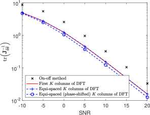
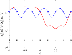
        (a) (b)

Figure 2: Bayesian CRB performance: $N=8$, $K=4$, and $L=2$: (a) Bayesian CRB for the overall parameter ${\mbox{\boldmath$\theta$\unboldmath}}=[\hbox{\boldmath$\alpha$\unboldmath}^{T},\hbox{\boldmath$\psi$\unboldmath}^{T}]^{T}$ and (b) Density of ${\bf J}_{\boldsymbol{\psi}\boldsymbol{\psi},D}$ over the angle domain (the same legend as in (a)).

The sum condition $\sum_{k=1}^{K}[{\bf W}]_{1,k}=0$ in Proposition 1 can be applied to previous designs including the DFT-based reflection patterns [21, 22]. This can be done by adjusting the first row elements of the reflection patterns so that the sum condition is satisfied. Fig. 2(a) shows the Bayesian CRB performance of several IRS reflection patterns for the estimation of the overall parameter $\alpha_{0},\alpha_{1},\cdots,\alpha_{L},\psi_{1},\cdots,\psi_{L}$ when the number of IRS elements $N=8$, the number of training symbols $K=4$, and the number of paths $L=2$. Here, the signal-to-noise ratio (SNR) is defined as $\mbox{SNR}=\rho/\sigma_{n}^{2}$. The on-off method switching the on-off states of the reflecting elements [19] shows degraded performance over the entire range of SNR. This is because the on-off switching method does not exploit all reflecting elements simultaneously for channel estimation. The orthogonal reflection patterns including the first $K$ columns [21, 22] and equi-spaced $K$ columns of the $N\times N$ DFT matrix yield improved performance as compared to the on-off method. We implemented the condition of Proposition 1 on the equi-spaced $K$ columns on the DFT matrix by progressively shifting the phases of the $K$ column vectors by $e^{j\frac{2\pi}{K}(k-1)}$, $k=1,2,\cdots,K$ so that $\sum_{k=1}^{K}[{\bf W}]_{1,k}=0$ (note that the first row of a DFT matrix is an all-one vector). Indeed, the phase-shifted equi-spaced $K$ columns of the DFT matrix shows further performance improvement, as seen in Fig. 2(a). Fig. 2(b) shows the quantity $2\frac{\partial}{\partial\psi}{\bf u}_{N}^{H}(\psi){\bf Q}\frac{\partial}{\partial\psi}{\bf u}_{N}(\psi)$ as a function of $\psi$ for the IRS reflection patterns considered in Fig. 2(a). Note that ${\bf J}_{\boldsymbol{\psi}\boldsymbol{\psi},D}$ in (46) whose inverse constitutes the lower diagonal block of $\text{tr}\bigl{(}{\bf J}_{\tilde{\boldsymbol{\theta}}\tilde{\boldsymbol{\theta}}}^{-1}\bigr{)}$ in (61) determining the angle estimation performance is given by ${\bf J}_{\boldsymbol{\psi}\boldsymbol{\psi},D}=\frac{\rho\sigma^{2}}{\sigma_{n}^{2}}{\mathbb{E}}_{\psi}\{2\frac{\partial}{\partial\psi}{\bf u}_{N}^{H}(\psi){\bf Q}\frac{\partial}{\partial\psi}{\bf u}_{N}(\psi)\}{\bf I}_{L}$, as seen in the proof of Theorem 1 in Appendix. Hence, $2\frac{\partial}{\partial\psi}{\bf u}_{N}^{H}(\psi){\bf Q}\frac{\partial}{\partial\psi}{\bf u}_{N}(\psi)$ shows the density of Fisher information over the angle domain before taking the expectation over $\psi_{\ell}\sim\mbox{Unif}[-1,1]$. High Fisher information density at a certain angle means high estimation performance (i.e., low estimation error) at that angle. It is seen that the Fisher information density is angle-dependent for the considered IRS reflection patterns. The first $4$ columns of the $8\times 8$ DFT matrix has high Fisher information density for $\psi\in[-1,0]$ and low Fisher information density for $\psi\in[0,1]$. This is because the first $4$ columns are equivalent to the orthogonal steering vectors to the look-angles in $[-1,0]$. On the other hand, the equi-spaced $4$ columns of the $8\times 8$ DFT matrix spreads out Fisher information over the entire angle range with some ripples. The phase-shifted equi-spaced DFT columns satisfying the condition in Proposition 1 has the same value of the integrated Fisher information as the equi-spaced DFT columns.

Method	Maximum (dB)	Minimum (dB)	Average (dB)
On-off method	24.4	24.4	24.4
First $K$ columns of DFT	43.2	30.8	40.4
Equi-spaced $K$ columns of DFT	42.3	37.0	40.4
Equi-spaced (phase-shifted) $K$ columns of DFT	42.3	37.0	40.4

TABLE I: Comparison of several IRS reflection patterns in terms of density of ${\bf J}_{\boldsymbol{\psi}\boldsymbol{\psi},D}$.

Table I summarizes the maximum, minimum, and average (i.e., integrated) values of $2\frac{\partial}{\partial\psi}{\bf u}_{N}^{H}(\psi){\bf Q}\frac{\partial}{\partial\psi}{\bf u}_{N}(\psi)$ over the angle domain for the same setup in Fig. 2. Note that all the reflection patterns other than the on-off method satisfy the constant modulus constraint and they have the same integrated Fisher information ${\mathbb{E}}_{\psi}\{2\frac{\partial}{\partial\psi}{\bf u}_{N}^{H}(\psi){\bf Q}\frac{\partial}{\partial\psi}{\bf u}_{N}(\psi)\}$ with $\psi_{\ell}\sim\mbox{Unif}[-1,1]$. At a particular path angle, however, the angle estimation performance can be different for each reflection pattern because the Fisher information density $2\frac{\partial}{\partial\psi}{\bf u}_{N}^{H}(\psi){\bf Q}\frac{\partial}{\partial\psi}{\bf u}_{N}(\psi)$ varies over the angle domain and has distinct peak-to-valley height, as seen in Fig. 2(b). This suggests that we can exploit the Fisher information density itself rather than its integrated value when we focus on the angle estimation performance considering the desired performance distribution over the angle domain. This will be investigated in the next section.

IV Hybrid CRB-based Reflection Pattern Design

To take advantage of the Fisher information density before taking expectation, we need deterministic parameter assumption. However, the full deterministic assumption for both path gains and path angles makes the derivation of CRB very difficult. We circumvent this difficulty with a hybrid parameter assumption. Since in sparse mmWave channels, the estimation of path angles is crucial to collect the propagation power spread in the space with beamforming and yield high SNR [38, 39], we now take the path angle parameter $\psi$ as a deterministic parameter (hence the expectation over $\psi$ is not taken) whereas we treat the path gain parameter $\alpha$ as a random nuisance parameter.

IV-A Derivation of Hybrid CRB

The FIM for the estimation of the random vector $\alpha$ and the deterministic vector $\psi$ can be obtained by averaging ${\bf y}$ and $\alpha$ out from the covariance matrix of the score function conditioned on $\psi$. Then, the derived CRB becomes a function of the path-angle parameter $\psi$ and thus yields a lower bound on the MSE of estimation for given true underlying parameter $\psi$. From the system model (9), the conditional pdf of ${\bf y}$ and $\alpha$ given $\psi$ is given by

$$p({\bf y},\hbox{\boldmath$\alpha$\unboldmath};\hbox{\boldmath$\psi$\unboldmath}) =p({\bf y}|\hbox{\boldmath$\alpha$\unboldmath};\hbox{\boldmath$\psi$\unboldmath})p(\hbox{\boldmath$\alpha$\unboldmath})=\frac{1}{\left(\pi\sigma_{n}^{2}\right)^{K}}\text{exp}\left(-\frac{1}{\sigma_{n}^{2}}\left\|{\bf y}-{\bf m}\right\|^{2}\right)p(\hbox{\boldmath$\alpha$\unboldmath}),$$ (69)

where ${\bf m}=\sqrt{\rho}\widetilde{{\bf W}}^{H}\left[\alpha_{0},{\bf h}^{T}\right]^{T}$ and ${\bf h}={\bf U}_{\boldsymbol{\psi}}[\alpha_{1},\cdots,\alpha_{L}]^{T}$. The CRB in this hybrid case is provided in the following theorem.

Theorem 2

Under the system model (9) with random path-gain parameter $\hbox{\boldmath$\alpha$\unboldmath}\sim\mathcal{CN}(\hbox{\boldmath$\mu$\unboldmath},\sigma^{2}{\bf I}_{L+1})$, $\hbox{\boldmath$\mu$\unboldmath}=[\mu_{0},\mathbf{0}_{L}^{T}]^{T}$, and deterministic path-angle parameter $\psi$, the hybrid CRB for any unbiased estimator of the overall parameter ${\mbox{\boldmath$\theta$\unboldmath}}=[\hbox{\boldmath$\alpha$\unboldmath}^{T},\hbox{\boldmath$\psi$\unboldmath}^{T}]^{T}$ is given by $\text{tr}\left(\breve{{\bf J}}_{\tilde{\boldsymbol{\theta}}\tilde{\boldsymbol{\theta}}}^{-1}\right)$, where $\breve{{\bf J}}_{\tilde{\boldsymbol{\theta}}\tilde{\boldsymbol{\theta}}}=\breve{{\bf J}}_{\tilde{\boldsymbol{\theta}}\tilde{\boldsymbol{\theta}},D}+\breve{{\bf J}}_{\tilde{\boldsymbol{\theta}}\tilde{\boldsymbol{\theta}},P}$. The two component matrices $\breve{{\bf J}}_{\tilde{\boldsymbol{\theta}}\tilde{\boldsymbol{\theta}},D}$ and $\breve{{\bf J}}_{\tilde{\boldsymbol{\theta}}\tilde{\boldsymbol{\theta}},P}$ of $\breve{{\bf J}}_{\tilde{\boldsymbol{\theta}}\tilde{\boldsymbol{\theta}}}$ are given by

$$\breve{{\bf J}}_{\tilde{\boldsymbol{\theta}}\tilde{\boldsymbol{\theta}},D} =\tilde{{\bf M}}\left[\begin{array}[]{cc|c}\breve{{\bf J}}_{\boldsymbol{\alpha}\boldsymbol{\alpha},D}&\mathbf{0}_{L+1}\mathbf{0}_{L+1}^{T}&\mathbf{0}_{L+1}\mathbf{0}_{L}^{T}\\ \mathbf{0}_{L+1}\mathbf{0}_{L+1}^{T}&\breve{{\bf J}}_{\boldsymbol{\alpha}\boldsymbol{\alpha},D}^{*}&\mathbf{0}_{L+1}\mathbf{0}_{L}^{T}\\ \hline\cr\mathbf{0}_{L}\mathbf{0}_{L+1}^{T}&\mathbf{0}_{L}\mathbf{0}_{L+1}^{T}&\breve{{\bf J}}_{\boldsymbol{\psi}\boldsymbol{\psi},D}\\ \end{array}\right]\tilde{{\bf M}}^{H}~{}~{}~{}\text{and}~{}~{}~{}\breve{{\bf J}}_{\tilde{\boldsymbol{\theta}}\tilde{\boldsymbol{\theta}},P}={\bf J}_{\tilde{\boldsymbol{\theta}}\tilde{\boldsymbol{\theta}},P},$$ (73)

where

$$\breve{{\bf J}}_{\boldsymbol{\alpha}\boldsymbol{\alpha},D} =\frac{\rho}{\sigma_{n}^{2}}\left[\begin{array}[]{cc}K&\bar{{\bf w}}^{H}{\bf U}_{\boldsymbol{\psi}}\\ {\bf U}_{\boldsymbol{\psi}}^{H}\bar{{\bf w}}&{\bf U}_{\boldsymbol{\psi}}^{H}{\bf Q}{\bf U}_{\boldsymbol{\psi}}\end{array}\right];~{}~{}~{}~{}~{}[\breve{{\bf J}}_{\boldsymbol{\psi}\boldsymbol{\psi},D}]_{p,q} =\left\{\begin{array}[]{ll}2\frac{\rho\sigma^{2}}{\sigma_{n}^{2}}\frac{\partial{\bf u}_{N}^{H}(\psi_{p})}{\partial\psi_{p}}{\bf Q}\frac{\partial{\bf u}_{N}(\psi_{q})}{\partial\psi_{q}},&\text{if }p=q\\ 0,&\text{if }p\neq q\end{array}\right.;$$ (78)

${\bf J}_{\tilde{\boldsymbol{\theta}}\tilde{\boldsymbol{\theta}},P}$, $\bar{{\bf w}}$ and ${\bf Q}$ are given in (31) and (37); and ${\bf u}_{N}(\cdot)$ is the ULA response vector.

Proof: See Appendix -D.

Note that in the hybrid case, the $p$-th diagonal element of $\breve{{\bf J}}_{\boldsymbol{\psi}\boldsymbol{\psi},D}$ is nothing but the Fisher information density at $\psi_{p}$, mentioned in the previous section. Since ${\bf J}_{\tilde{\boldsymbol{\theta}}\tilde{\boldsymbol{\theta}},P}~{}(=\breve{{\bf J}}_{\tilde{\boldsymbol{\theta}}\tilde{\boldsymbol{\theta}},P})$ is block-diagonal, as seen in (31), with its constituent matrices ${\bf J}_{{\boldsymbol{\alpha}}{\boldsymbol{\alpha}},P}=\frac{1}{\sigma^{2}}{\bf I}_{L+1}$ and ${\bf J}_{{\boldsymbol{\psi}}{\boldsymbol{\psi}},P}={\mathbf{0}}_{L}{\mathbf{0}}_{L}^{T}$, the hybrid FIM $\breve{{\bf J}}_{\tilde{\boldsymbol{\theta}}\tilde{\boldsymbol{\theta}}}$ has a block-diagonal form and we have separate sub-FIMs for the path gains and the path angles, as seen in (73). Thus, the MSE lower bound for the estimation of the path-angle parameter $\psi$ is determined by the inverse of the lower diagonal block $\breve{{\bf J}}_{\boldsymbol{\psi}\boldsymbol{\psi},D}$ due to $\breve{{\bf J}}_{{\boldsymbol{\psi}}{\boldsymbol{\psi}},P}={\mathbf{0}}_{L}{\mathbf{0}}_{L}^{T}$, whereas the MSE lower bound for the estimation of the path-gain parameter $\alpha$ is determined by the upper diagonal element $\breve{{\bf J}}_{\boldsymbol{\alpha}\boldsymbol{\alpha}}=\breve{{\bf J}}_{\boldsymbol{\alpha}\boldsymbol{\alpha},D}+\breve{{\bf J}}_{\boldsymbol{\alpha}\boldsymbol{\alpha},P}$. Both of the FIM submatrices are functions of the design variable ${\bf Q}~{}(={\bf W}{\bf W}^{H})$ and the true angle parameter $\psi$. Focusing on the path-angle parameter while treating the path-gain parameter as a nuisance parameter, we can optimize the IRS reflection matrix ${\bf W}$ in order to yield the best angle-estimation CRB based on $\breve{{\bf J}}_{\boldsymbol{\psi}\boldsymbol{\psi},D}$. (Note that in (73), the lower diagonal block of $\tilde{{\bf M}}$ multiplied to $\breve{{\bf J}}_{\boldsymbol{\psi}\boldsymbol{\psi},D}$ is the identity matrix, as seen in (22).)

IV-B Hybrid CRB-based Reflection Pattern

As seen in Theorem 2, the FIM submatrix $\breve{{\bf J}}_{\boldsymbol{\psi}\boldsymbol{\psi},D}$ determining the performance of path angle estimation is a function of the design variable ${\bf Q}~{}(={\bf W}{\bf W}^{H})$ and the true underlying path angle $\psi$. A key point to note is that the CRB $\mbox{tr}\left(\breve{{\bf J}}^{-1}_{\boldsymbol{\psi}\boldsymbol{\psi},D}\right)$ determines the estimation performance when the true path angles are $\hbox{\boldmath$\psi$\unboldmath}=[\psi_{1},\cdots,\psi_{L}]^{T}$. Hence, our design approach with the hybrid CRB is that we first design a set of targeted look-angles and then optimize ${\bf W}$ so that ${\bf W}$ yields best estimation performance when the true path angles are at the targeted look-angles. Here, we can exploit some side information about the path angles if any, e.g., its support information $\psi_{\ell}\in[\Delta_{1},\Delta_{2}],~{}\forall\ell$. With such information, we design the set of targeted look-angles as $\xi_{L_{T},\ell}\in\left\{\Delta_{1}+\frac{\Delta_{2}-\Delta_{1}}{L_{T}}(\ell-1)~{}|~{}\ell=1,\ldots,L_{T}\right\}$, i.e., the targeted look-angles are evenly spaced over the entire angle range $[\Delta_{1},\Delta_{2}]$ with $L_{T}$ angles. Then, the optimization problem is formulated as

$$\min_{{\bf W}} \text{tr}\left(\breve{{\bf J}}^{-1}_{\boldsymbol{\psi}\boldsymbol{\psi},D}\left|\boldsymbol{\psi}=\hbox{\boldmath$\xi$\unboldmath}{\stackrel{{\scriptstyle\Delta}}{{=}}}[\xi_{L_{T},1},\cdots,\xi_{L_{T},L_{T}}]\right.\right)$$ (79)

subject to $$|[{\bf W}]_{p,q}|=\sqrt{\beta},~{}~{}~{}\forall p,q.$$ (80)

Remark 3

Using the Cauchy-Schwartz inequality $\left(\sum_{\ell=1}^{L}\sqrt{\lambda_{\ell}}\frac{1}{\sqrt{\lambda_{\ell}}}\right)^{2}\leq\sum_{\ell=1}^{L}\lambda_{\ell}\cdot\sum_{\ell=1}^{L}\frac{1}{\lambda_{\ell}}$, where $\lambda_{\ell}=2\frac{\rho\sigma^{2}}{\sigma_{n}^{2}}\frac{\partial{\bf u}_{N}^{H}(\psi_{\ell})}{\partial\psi_{\ell}}{\bf Q}\frac{\partial{\bf u}_{N}(\psi_{\ell})}{\partial\psi_{\ell}}$, we have the following inequality regarding the trace of the inverse of $\breve{{\bf J}}_{\boldsymbol{\psi}\boldsymbol{\psi},D}$:

$$\text{tr}\left(\breve{{\bf J}}_{{\boldsymbol{\psi}}{\boldsymbol{\psi}},D}^{-1}\right)\geq L^{2}\left[\text{tr}\left(\breve{{\bf J}}_{{\boldsymbol{\psi}}{\boldsymbol{\psi}},D}\right)\right]^{-1}~{}~{}~{}\mbox{for any true }\hbox{\boldmath$\psi$\unboldmath}.$$ (81)

The equality is achieved if and only if $\lambda_{1}=\cdots=\lambda_{L}$. This condition can be achieved by ${\bf Q}={\bf W}{\bf W}^{H}=K\beta{\bf I}_{N}$ if $K\geq N$. That is, with ${\bf Q}=K\beta{\bf I}_{N}$, $\lambda_{\ell}=2K\beta\frac{\rho\sigma^{2}}{\sigma_{n}^{2}}\frac{\partial{\bf u}_{N}^{H}(\psi_{\ell})}{\partial\psi_{\ell}}\frac{\partial{\bf u}_{N}(\psi_{\ell})}{\partial\psi_{\ell}}$ $=2K\beta\frac{\rho\sigma^{2}}{\sigma_{n}^{2}}\sum_{m=1}^{N-1}m^{2}$ does not depend on the index $\ell$. (Please see in (99) in Appendix -A regarding $\frac{\partial{\bf u}_{N}(\psi_{\ell})}{\partial\psi_{\ell}}$.) So, we can see the optimality of ${\bf Q}=K\beta{\bf I}_{N}$ obtained in the previous work [21, 22] in the case of $K\geq N$ in this sense too.

Since our main focus in this paper is sparse mmWave channels, the situation is $L\leq K<N$. We consider the optimization problem (79) - (80) in the case of $K<N$. The objective function (79) can be rewritten as

$$\text{tr}\left(\breve{{\bf J}}_{{\boldsymbol{\psi}}{\boldsymbol{\psi}},D}^{-1}\left|\hbox{\boldmath$\psi$\unboldmath}=\hbox{\boldmath$\xi$\unboldmath}\right.\right) =\frac{\sigma_{n}^{2}}{2\rho\sigma^{2}}\sum_{\ell=1}^{L_{T}}\frac{1}{\text{tr}\left({\bf W}^{H}\frac{\partial{\bf u}_{N}(\xi_{L_{T},\ell})}{\partial\xi_{L_{T},\ell}}\frac{\partial{\bf u}_{N}^{H}(\xi_{L_{T},\ell})}{\partial\xi_{L_{T},\ell}}{\bf W}\right)}$$ (82)

$$\stackrel{{\scriptstyle(a)}}{{=}}\frac{\sigma_{n}^{2}}{2\rho\sigma^{2}}\sum_{\ell=1}^{L_{T}}\frac{1}{\text{vec}\left(\frac{\partial{\bf u}_{N}^{H}(\xi_{L_{T},\ell})}{\partial\xi_{L_{T},\ell}}{\bf W}\right)^{H}\text{vec}\left(\frac{\partial{\bf u}_{N}^{H}(\xi_{L_{T},\ell})}{\partial\xi_{L_{T},\ell}}{\bf W}\right)}$$ (83)

$$\stackrel{{\scriptstyle(b)}}{{=}}\frac{\sigma_{n}^{2}}{2\rho\sigma^{2}}\sum_{\ell=1}^{L_{T}}\frac{1}{\overrightarrow{{\bf w}}^{H}\left({\bf I}_{K}\otimes\frac{\partial{\bf u}_{N}(\xi_{L_{T},\ell})}{\partial\xi_{L_{T},\ell}}\frac{\partial{\bf u}_{N}^{H}(\xi_{L_{T},\ell})}{\partial\xi_{L_{T},\ell}}\right)\overrightarrow{{\bf w}}}~{}{\stackrel{{\scriptstyle\Delta}}{{=}}}~{}f(\overrightarrow{{\bf w}}),$$ (84)

where $\overrightarrow{{\bf w}}=\text{vec}({\bf W})$, Step $(a)$ is valid due to $\text{tr}({\bf A}^{H}{\bf B})=\text{vec}({\bf A})^{H}\text{vec}({\bf B})$, and Step $(b)$ is valid because $\text{vec}({\bf A}{\bf X}{\bf B})=({\bf B}^{T}\otimes{\bf A})\text{vec}({\bf X})$ and $({\bf A}_{1}\otimes{\bf B}_{1})({\bf A}_{2}\otimes{\bf B}_{2})=({\bf A}_{1}{\bf A}_{2}\otimes{\bf B}_{1}{\bf B}_{2})$. Thus, the objective function is the sum of the inverses of Rayleigh quotients since $\overrightarrow{{\bf w}}^{H}\overrightarrow{{\bf w}}=NK\beta$ under the constant modulus constraint $|[{\bf W}]_{p,q}|=\sqrt{\beta},\forall p,q$. It is known that even the optimization of the sum of Rayleigh quotients is not a simple problem. In our case, we have the sum of the inverses of Rayleigh quotients and the elementwise constant modulus constraint in addition. To tackle this optimization problem, we adopt the PGM [23, 24]. PGM is an iterative method applying gradient descent and projection onto the constraint set in an alternating manner and is suited to complicated constraints. The overall algorithm is summarized in Algorithm 1. The objective function (84) is differentiable and its Wirtinger complex gradient is given by

$$\nabla_{\overrightarrow{{\bf w}}^{*}}f(\overrightarrow{{\bf w}}) =-\sum_{\ell=1}^{L_{T}}\frac{\left({\bf I}_{K}\otimes\frac{\partial{\bf u}_{N}(\xi_{L_{T},\ell})}{\partial\xi_{L_{T},\ell}}\frac{\partial{\bf u}_{N}^{H}(\xi_{L_{T},\ell})}{\partial\xi_{L_{T},\ell}}\right)}{\left[\overrightarrow{{\bf w}}^{H}\left({\bf I}_{K}\otimes\frac{\partial{\bf u}_{N}(\xi_{L_{T},\ell})}{\partial\xi_{L_{T},\ell}}\frac{\partial{\bf u}_{N}^{H}(\xi_{L_{T},\ell})}{\partial\xi_{L_{T},\ell}}\right)\overrightarrow{{\bf w}}\right]^{2}}\overrightarrow{{\bf w}}.$$ (85)

We start with an initial point $\overrightarrow{{\bf w}}^{(0)}$. At the $i$-th iteration, we update the current $\overrightarrow{{\bf w}}^{(i)}$ by using gradient descent based on the gradient vector (85) and then project the updated vector onto the constraint set ${\cal C}:=\left\{\overrightarrow{{\bf w}}=[w_{1},\ldots,w_{KN}]^{T}\in\mathbb{C}^{KN}:|w_{i}|=\sqrt{\beta}\right\}$. We repeat this iteration. In the step size determination, we apply the technique in [40] to mitigate the slow crawling problem of gradient decent near a local minimum and help escape from local stationary points of the objective function. That is, we normalize the magnitude of each component of the gradient vector by multiplying the $i$-th component of the gradient vector by its magnitude inverse, as seen in Line 5 of Algorithm 1.

Algorithm 1 The Proposed PGM-based IRS Reflection Pattern Design

0:  Stopping criterion $\epsilon$, step size $\delta$, and targeted look-angles $\{\xi_{L_{T},\ell}\}$

1:  Compute $\frac{\partial{\bf u}_{N}(\xi_{L_{T},\ell})}{\partial\xi_{L_{T},\ell}}$ for $\ell=1,\cdots,L_{T}$.

2:  Set $i=0$ and initialize $\overrightarrow{{\bf w}}^{(0)}$.

3:  repeat

4:     Compute the gradient vector (85) at $\overrightarrow{{\bf w}}^{(i)}$.

5:     Update $\overrightarrow{{\bf w}}^{(i+1)}=\Pi_{{\cal C}}\left(\overrightarrow{{\bf w}}^{(i)}-{\bf r}_{i}\odot\nabla_{\overrightarrow{{\bf w}}^{*}}f(\overrightarrow{{\bf w}}^{(i)})\right)$, where $\Pi_{{\cal C}}$ is the projection onto ${\cal C}$; ${\bf r}_{i}=\left[\frac{\delta}{\left|\left[\nabla_{\overrightarrow{{\bf w}}^{*}}f(\overrightarrow{{\bf w}}^{(i)})\right]_{1}\right|},\cdots,\frac{\delta}{\left|\left[\nabla_{\overrightarrow{{\bf w}}^{*}}f(\overrightarrow{{\bf w}}^{(i)})\right]_{NK}\right|}\right]^{T}$; and $\odot$ denotes elementwise multiplication.

6:     $i=i+1$

7:  until $\left\|\overrightarrow{{\bf w}}^{(i)}-\overrightarrow{{\bf w}}^{(i-1)}\right\|^{2}/\left\|\overrightarrow{{\bf w}}^{(i-1)}\right\|^{2}\leq\epsilon$

V Numerical Results

In this section, we provide numerical results to evaluate the proposed IRS reflection pattern design. During the simulation, we set the magnitude of the reflection coefficient of each element at the IRS as $\beta=1$. We used the channel model (3), where the number of the IRS-assisted channel paths was set $L\in\{1,\ldots,4\}$, $\alpha_{0}\sim{\cal C}{\cal N}(\mu_{0},\sigma^{2})$ and $\alpha_{\ell}\stackrel{{\scriptstyle i.i.d.}}{{\sim}}{\cal C}{\cal N}(0,\sigma^{2})$, $\ell=1,\cdots,L$ with $\mu_{0}=\sigma^{2}=1$. The SNR is given by $\mbox{SNR}=\rho/\sigma_{n}^{2}$.

     
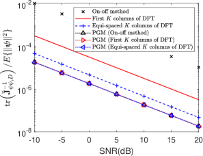
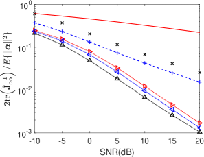
(a) (b) (c) (d)

           

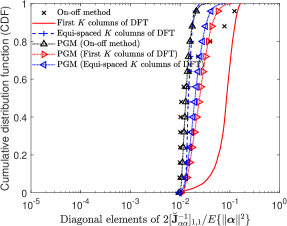
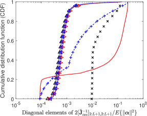
Figure 3: Hybrid CRB comparision with several IRS reflection patterns versus SNR where $N=32$, $K=8$, and $L=3$ (PGM represents the proposed design with the initial pattern for Algorithm 1 which is shown in the parenthesis.): (a) $\mbox{tr}\bigl{(}\breve{{\bf J}}_{\boldsymbol{\psi}\boldsymbol{\psi},D}^{-1}\bigr{)}/\mathbb{E}\{\|\boldsymbol{\psi}\|^{2}\}$, (b) $\bigl{(}\mbox{tr}\bigl{(}\breve{{\bf J}}_{\boldsymbol{\alpha}\boldsymbol{\alpha}}^{-1}\bigr{)}+\mbox{tr}\bigl{(}\breve{{\bf J}}_{\boldsymbol{\alpha}^{*}\boldsymbol{\alpha}^{*}}^{-1}\bigr{)}\bigr{)}/\mathbb{E}\{\|\boldsymbol{\alpha}\|^{2}\}$, (c) $\bigl{(}[\breve{{\bf J}}_{\boldsymbol{\alpha}\boldsymbol{\alpha}}^{-1}]_{1,1}+[\breve{{\bf J}}_{\boldsymbol{\alpha}^{*}\boldsymbol{\alpha}^{*}}^{-1}]_{1,1}\bigr{)}/\mathbb{E}\{\|\boldsymbol{\alpha}\|^{2}\}$ at $\text{SNR}=5$dB, and (d) $\text{diag}\bigl{(}[\breve{{\bf J}}_{\boldsymbol{\alpha}\boldsymbol{\alpha}}^{-1}]_{2:L+1,2:L+1}+[\breve{{\bf J}}_{\boldsymbol{\alpha}^{*}\boldsymbol{\alpha}^{*}}^{-1}]_{2:L+1,2:L+1}\bigr{)}/\mathbb{E}\{\|\boldsymbol{\alpha}\|^{2}\}$ at $\text{SNR}=5$dB. (The subfigures (a)-(d) have the same legend.)

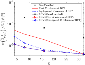
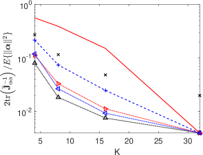
     (a) Hybrid CRB for $\psi$ (b) Hybrid CRB for $\alpha$ (same legend as in (a))

Figure 4: Hybrid CRB comparision with several IRS reflection patterns versus $K$ where $N=32$, $L=3$, and $\text{SNR}=5$dB.

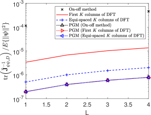
     (a) Hybrid CRB for $\psi$ (b) Hybrid CRB for $\alpha$ (same legend as in (a))

Figure 5: Hybrid CRB comparision with several IRS reflection patterns versus $L$ where $N=32$, $K=8$, and $\text{SNR}=5$dB.

We considered the case of $N=32$ and $K=8$. We designed the IRS pattern matrix by running Algorithm 1 with $\epsilon=10^{-10}$, $\delta=1$, and $L_{T}=N$ targeted look-angles evenly spaced over $[-1,1]$. Then, we generated $\psi_{\ell}\stackrel{{\scriptstyle i.i.d.}}{{\sim}}\text{Unif}[-1,1]$, $\ell=1,\cdots,L$ and computed $\mbox{tr}(\breve{{\bf J}}^{-1}_{\boldsymbol{\psi}\boldsymbol{\psi},D})$ and $\mbox{tr}(\breve{{\bf J}}^{-1}_{\boldsymbol{\alpha}\boldsymbol{\alpha}})$ with $\breve{{\bf J}}_{\boldsymbol{\alpha}\boldsymbol{\alpha}}=\breve{{\bf J}}_{\boldsymbol{\alpha}\boldsymbol{\alpha},D}+\breve{{\bf J}}_{\boldsymbol{\alpha}\boldsymbol{\alpha},P}$ by using the designed ${\bf W}$ and the generated true angles $\psi_{1},\cdots,\psi_{L}$. We repeated this procedure for $5000$ random channel realizations and then took average over the $5000$ Monte Carlo runs. Hence, this angle estimation performance average corresponds to ${\mathbb{E}}_{\boldsymbol{\psi}}\{\breve{{\bf J}}^{-1}_{\boldsymbol{\psi}\boldsymbol{\psi},D}\}$, i.e., the bound (a) not the bound (b) in (11). For other IRS pattern matrix designs, we applied the same Monte Carlo evaluation. The result is shown in Fig. 3. It is seen in Fig. 3(a) that the equi-spaced $K$ DFT columns shows better performance than the on-off method and the first $K$ DFT columns since $\psi_{\ell}$ is distributed over the angle range $[-1,1]$. It is also seen that the proposed design yields noticeable gain over the equi-spaced $K$ DFT columns. Note that the first $K$ DFT columns and the equi-spaced $K$ DFT columns show different performance here, whereas the two methods shows the same performance in Fig. 2(a). This is because Fig. 3(a) shows the tighter bound (a) in (11), whereas Fig. 2(a) shows the looser bound (b) in (11). Fig. 3(b) shows the corresponding path-gain CRB $\mbox{tr}(\breve{{\bf J}}^{-1}_{\boldsymbol{\alpha}\boldsymbol{\alpha}})$ averaged over the Monte Carlo runs. It is seen that the first $K$ DFT columns shows severe performance degradation in path gain estimation. This is because this method has a heavy tail in the error distribution due to large gain estimation error occurring when the realized path angles are not within the coverage of the first $K$ DFT columns, as seen in Figs. 3(c) and (d).

Then, we evaluated the hybrid CRB performance of the IRS reflection patterns with different values of $K$. Fig. 4 shows that the designs using the orthogonal DFT matrix achieve the best performance when $K=N$ as expected, but there is noticeable gain by the proposed design method as $K$ decreases from $N$. Finally, we examined the performance of the proposed method with respect to the number of channel paths $L$ and the result is shown in Fig. 5. It is seen that the CRB performance degrades as $L$ increases due to the increased number of parameters to estimate. It is also seen that the design by Algorithm 1 yields better performance than other methods.

VI Conclusion

We have considered the problem of training signal design for IRS-assisted mmWave communication under a sparse channel model. We have approached the problem based on CRB for channel estimation. With the full Bayesian approach, we have shown that the main factor affecting the angle estimation performance is the Fisher information density given by a quadratic form composed of the derivative of the ULA response and the IRS reflection pattern matrix square ${\bf Q}$. Based on this fact, we have approached the IRS pattern matrix design problem with a hybrid CRB under the assumption of random path gains and unknown deterministic path angles. We have proposed a PGM-based algorithm to solve optimal IRS pattern matrix design focusing on the path angle estimation critical in mmWave communication. We have validated the effectiveness of the proposed design method with numerical evaluation. We can consider the following future works. First, in this paper we fixed $s_{k}=\sqrt{\rho}$ to simplify the problem. The joint design of the training symbol sequence and the IRS reflection pattern matrix remains as a future work. Next, development of estimation algorithms achieving the CRB under the signal model (9) should be studied as future work.

-A Proof of Theorem 1

Step 1: To prove Theorem 1, we first provide the following lemma. Note that in the Bayesian case we need the expectation of the second order derivatives of the logarithm of $p({\bf y},{\mbox{\boldmath$\theta$\unboldmath}})$ with ${\mbox{\boldmath$\theta$\unboldmath}}=[\hbox{\boldmath$\alpha$\unboldmath}^{T},\hbox{\boldmath$\psi$\unboldmath}^{T}]^{T}$, as seen in (13) - (23). The logarithm of $p({\bf y},{\mbox{\boldmath$\theta$\unboldmath}})$ is decomposed as $\ln p({\bf y},{\mbox{\boldmath$\theta$\unboldmath}})=\ln p({\mbox{\boldmath$\theta$\unboldmath}})+\ln p({\bf y}|{\mbox{\boldmath$\theta$\unboldmath}})$ as seen in (12), and Lemma 2 provides the second order derivatives of $\ln p({\bf y}|{\mbox{\boldmath$\theta$\unboldmath}})$.

Lemma 2

The second-order derivatives of the log-likelihood function $\ln p({\bf y}|\boldsymbol{\theta})$ under the observation model (9) are given by

$$\frac{\partial}{\partial\boldsymbol{\alpha}^{*}}\left(\frac{\partial\ln p({\bf y}|\boldsymbol{\theta})}{\partial\boldsymbol{\alpha}^{*}}\right)^{H}=-\frac{\rho}{\sigma_{n}^{2}}\left[\begin{array}[]{cc}K&\bar{{\bf w}}^{H}{\bf U}_{\boldsymbol{\psi}}\\ {\bf U}_{\boldsymbol{\psi}}^{H}\bar{{\bf w}}&{\bf U}_{\boldsymbol{\psi}}^{H}{\bf Q}{\bf U}_{\boldsymbol{\psi}}\end{array}\right]=\left(\frac{\partial}{\partial\boldsymbol{\alpha}}\left(\frac{\partial\ln p({\bf y}|\boldsymbol{\theta})}{\partial\boldsymbol{\alpha}}\right)^{H}\right)^{*}$$ (88)

$$\frac{\partial}{\partial\psi_{p}}\left(\frac{\partial\ln p({\bf y}|\boldsymbol{\theta})}{\partial\psi_{q}}\right)^{H}$$

$$=-\frac{1}{\sigma_{n}^{2}}\left(-({\bf y}-{\bf m})^{H}\frac{\partial^{2}{\bf m}}{\partial\psi_{p}\partial\psi_{q}}+\frac{\partial{\bf m}^{H}}{\partial\psi_{p}}\frac{\partial{\bf m}}{\partial\psi_{q}}+\frac{\partial{\bf m}^{H}}{\partial\psi_{q}}\frac{\partial{\bf m}}{\partial\psi_{p}}-\frac{\partial^{2}{\bf m}^{H}}{\partial\psi_{p}\partial\psi_{q}}({\bf y}-{\bf m})\right)$$ (89)

$$\frac{\partial}{\partial\boldsymbol{\alpha}^{*}}\left(\frac{\partial\ln p({\bf y}|\boldsymbol{\theta})}{\partial\psi_{\ell}}\right)^{H}$$

$$=-\frac{1}{\sigma_{n}^{2}}\left(-\sqrt{\rho}\widetilde{{\bf U}}_{\psi_{\ell}}^{H}\widetilde{{\bf W}}\left({\bf y}-\sqrt{\rho}\widetilde{{\bf W}}^{H}\left[\begin{array}[]{cc}1&\\ &{\bf U}_{\boldsymbol{\psi}}\end{array}\right]\boldsymbol{\alpha}\right)+\rho\left[\begin{array}[]{cc}K&\bar{{\bf w}}^{H}\\ {\bf U}_{\boldsymbol{\psi}}^{H}\bar{{\bf w}}&{\bf U}_{\boldsymbol{\psi}}^{H}{\bf Q}\end{array}\right]\widetilde{{\bf U}}_{\psi_{\ell}}\hbox{\boldmath$\alpha$\unboldmath}\right)$$ (94)

$$=\left(\frac{\partial}{\partial\boldsymbol{\alpha}}\left(\frac{\partial\ln p({\bf y}|\boldsymbol{\theta})}{\partial\psi_{\ell}}\right)^{H}\right)^{*}=\left(\frac{\partial}{\partial\psi_{\ell}}\left(\frac{\partial\ln p({\bf y}|\boldsymbol{\theta})}{\partial\boldsymbol{\alpha}^{*}}\right)^{H}\right)^{H}=\left(\frac{\partial}{\partial\psi_{\ell}}\left(\frac{\partial\ln p({\bf y}|\boldsymbol{\theta})}{\partial\boldsymbol{\alpha}}\right)^{H}\right)^{T}$$ (95)

$$\frac{\partial}{\partial\boldsymbol{\alpha}^{*}}\left(\frac{\partial\ln p({\bf y}|\boldsymbol{\theta})}{\partial\boldsymbol{\alpha}}\right)^{H}=\frac{\partial}{\partial\boldsymbol{\alpha}}\left(\frac{\partial\ln p({\bf y}|\boldsymbol{\theta})}{\partial\boldsymbol{\alpha}^{*}}\right)^{H}=\mathbf{0}_{L+1}\mathbf{0}_{L+1}^{T},$$ (96)

where

$$\widetilde{{\bf U}}_{\psi_{\ell}} \stackrel{{\scriptstyle\triangle}}{{=}}\left[\begin{array}[]{cc}\mathbf{0}_{N+1},&[0,\cdots,0,\underbrace{1}_{\tiny\ell^{th}},0,\cdots,0]\otimes\left[0,~{}\frac{\partial{\bf u}_{N}^{T}(\psi_{\ell})}{\partial\psi_{\ell}}\right]^{T}\end{array}\right]\in\mathbb{C}^{(N+1)\times(L+1)}$$ (98)

$$\frac{\partial{\bf u}_{N}(\psi)}{\partial\psi} \stackrel{{\scriptstyle\triangle}}{{=}}\iota\pi\left[0,e^{\iota\pi\psi},2e^{\iota 2\pi\psi},\ldots,(N-1)e^{\iota(N-1)\pi\psi}\right]^{T},$$ (99)

and the variables of $\bar{{\bf w}}$ and ${\bf Q}$ are defined in (37).

Proof: By differentiating $\ln p({\bf y}|\boldsymbol{\theta})$ in (12) w.r.t. $\alpha$ and $\psi$, we have

$$\frac{\partial\ln p({\bf y}|\boldsymbol{\theta})}{\partial\boldsymbol{\alpha}^{*}} =-\frac{1}{\sigma_{n}^{2}}\left(-\sqrt{\rho}\left[\begin{array}[]{cc}1&\\ &{\bf U}^{H}_{\boldsymbol{\psi}}\end{array}\right]\widetilde{{\bf W}}{\bf y}+\rho\left[\begin{array}[]{cc}1&\\ &{\bf U}^{H}_{\boldsymbol{\psi}}\end{array}\right]\widetilde{{\bf W}}\widetilde{{\bf W}}^{H}\left[\begin{array}[]{cc}1&\\ &{\bf U}_{\boldsymbol{\psi}}\end{array}\right]\hbox{\boldmath$\alpha$\unboldmath}\right)$$ (106)

$$=\left(\frac{\partial\ln p({\bf y}|\boldsymbol{\theta})}{\partial\boldsymbol{\alpha}}\right)^{*}$$ (107)

$$\frac{\partial\ln p({\bf y}|\boldsymbol{\theta})}{\partial\psi_{\ell}} =-\frac{1}{\sigma_{n}^{2}}\left(-({\bf y}-{\bf m})^{H}\frac{\partial{\bf m}}{\partial\psi_{\ell}}-\frac{\partial{\bf m}^{H}}{\partial\psi_{\ell}}({\bf y}-{\bf m})\right)$$ (108)

$$=-\frac{1}{\sigma_{n}^{2}}\biggl{(}-\sqrt{\rho}{\bf y}^{H}\widetilde{{\bf W}}^{H}\widetilde{{\bf U}}_{\psi_{\ell}}\hbox{\boldmath$\alpha$\unboldmath}-\sqrt{\rho}\hbox{\boldmath$\alpha$\unboldmath}^{H}\widetilde{{\bf U}}_{\psi_{\ell}}^{H}\widetilde{{\bf W}}{\bf y}$$

$$\hskip 70.0001pt+\rho\hbox{\boldmath$\alpha$\unboldmath}^{H}\left[\begin{array}[]{cc}1&\\ &{\bf U}^{H}_{\boldsymbol{\psi}}\end{array}\right]\widetilde{{\bf W}}\widetilde{{\bf W}}^{H}\widetilde{{\bf U}}_{\psi_{\ell}}\hbox{\boldmath$\alpha$\unboldmath}+\rho\hbox{\boldmath$\alpha$\unboldmath}^{H}\widetilde{{\bf U}}_{\psi_{\ell}}^{H}\widetilde{{\bf W}}\widetilde{{\bf W}}^{H}\left[\begin{array}[]{cc}1&\\ &{\bf U}_{\boldsymbol{\psi}}\end{array}\right]\hbox{\boldmath$\alpha$\unboldmath}\biggr{)}.$$ (113)

By differentiating (107) and (108) w.r.t. $\alpha$ and $\psi$ again, we have

$$\frac{\partial}{\partial\boldsymbol{\alpha}^{*}}\left(\frac{\partial\ln p({\bf y}|\boldsymbol{\theta})}{\partial\boldsymbol{\alpha}^{*}}\right)^{H} =-\frac{\rho}{\sigma_{n}^{2}}\left[\begin{array}[]{cc}1&\\ &{\bf U}^{H}_{\boldsymbol{\psi}}\end{array}\right]\left[\begin{array}[]{cc}K&\bar{{\bf w}}^{H}\\ \bar{{\bf w}}&{\bf Q}\end{array}\right]\left[\begin{array}[]{cc}1&\\ &{\bf U}_{\boldsymbol{\psi}}\end{array}\right]$$ (120)

$$\frac{\partial}{\partial\boldsymbol{\alpha}}\left(\frac{\partial\ln p({\bf y}|\boldsymbol{\theta})}{\partial\boldsymbol{\alpha}}\right)^{H} =-\frac{\rho}{\sigma_{n}^{2}}\left[\begin{array}[]{cc}1&\\ &{\bf U}^{T}_{\boldsymbol{\psi}}\end{array}\right]\left[\begin{array}[]{cc}K&\bar{{\bf w}}^{T}\\ \bar{{\bf w}}^{*}&{\bf Q}^{*}\end{array}\right]\left[\begin{array}[]{cc}1&\\ &{\bf U}^{*}_{\boldsymbol{\psi}}\end{array}\right]$$ (127)

$$\frac{\partial}{\partial\boldsymbol{\alpha}^{*}}\left(\frac{\partial\ln p({\bf y}|\boldsymbol{\theta})}{\partial\boldsymbol{\alpha}}\right)^{H} =\frac{\partial}{\partial\boldsymbol{\alpha}}\left(\frac{\partial\ln p({\bf y}|\boldsymbol{\theta})}{\partial\boldsymbol{\alpha}^{*}}\right)^{T}=\mathbf{0}_{L+1}\mathbf{0}_{L+1}^{T},$$ (128)

and the expression for $\frac{\partial}{\partial\psi_{p}}\left(\frac{\partial\ln p({\bf y}|\boldsymbol{\theta})}{\partial\psi_{q}}\right)^{H}$ is given in (89), which can further be detailed like (113). (The detailed expression is omitted due to space limitation.) By using (107) and (113), the mixed second-order partial derivative is similarly derived as

$$\frac{\partial}{\partial\boldsymbol{\alpha}^{*}}\left(\frac{\partial\ln p({\bf y}|\boldsymbol{\theta})}{\partial\psi_{\ell}}\right)^{H} =-\frac{1}{\sigma_{n}^{2}}\left[-\sqrt{\rho}\widetilde{{\bf U}}_{\psi_{\ell}}^{H}\widetilde{{\bf W}}\left({\bf y}-\sqrt{\rho}\widetilde{{\bf W}}^{H}\left[\begin{array}[]{cc}1&\\ &{\bf U}_{\boldsymbol{\psi}}\end{array}\right]\boldsymbol{\alpha}\right)\right.$$ (131)

$$\left.~{}~{}~{}~{}~{}~{}~{}~{}~{}~{}~{}+\rho\left[\begin{array}[]{cc}1&\\ &{\bf U}_{\boldsymbol{\psi}}^{H}\end{array}\right]\widetilde{{\bf W}}\widetilde{{\bf W}}^{H}\widetilde{{\bf U}}_{\psi_{\ell}}\hbox{\boldmath$\alpha$\unboldmath}\right],$$ (134)

and the expressions for $\frac{\partial}{\partial\boldsymbol{\alpha}}\left(\frac{\partial\ln p({\bf y}|\boldsymbol{\theta})}{\partial\psi_{\ell}}\right)^{H}$, $\frac{\partial}{\partial\psi_{\ell}}\left(\frac{\partial\ln p({\bf y}|\boldsymbol{\theta})}{\partial\boldsymbol{\alpha}^{*}}\right)^{H}$, and $\frac{\partial}{\partial\psi_{\ell}}\left(\frac{\partial\ln p({\bf y}|\boldsymbol{\theta})}{\partial\boldsymbol{\alpha}}\right)^{H}$ are given in (95). $\blacksquare$

Step 2: The FIM ${\bf J}_{\tilde{\boldsymbol{\theta}}\tilde{\boldsymbol{\theta}}}$ is obtained by applying $-\mathbb{E}_{{\bf y},\boldsymbol{\theta}}\{\cdot\}$ to the second-order derivatives of $\ln p({\bf y},{\mbox{\boldmath$\theta$\unboldmath}})=\ln p({\mbox{\boldmath$\theta$\unboldmath}})+\ln p({\bf y}|{\mbox{\boldmath$\theta$\unboldmath}})$. First, consider the log-likelihood part ${\bf J}_{\tilde{\boldsymbol{\theta}}\tilde{\boldsymbol{\theta}},D}$ for which the second-order derivatives are given in Lemma 2. The corresponding submatrices are given as

$${\bf J}_{\boldsymbol{\alpha}\boldsymbol{\alpha},D} =-\mathbb{E}_{{\bf y},\boldsymbol{\theta}}\left\{\frac{\partial}{\partial\boldsymbol{\alpha}^{*}}\left(\frac{\partial\ln p({\bf y}|\boldsymbol{\theta})}{\partial\boldsymbol{\alpha}^{*}}\right)^{H}\right\}=\frac{\rho}{\sigma_{n}^{2}}\left[\begin{array}[]{cc}K&\nu_{1}^{*}\mathbf{1}_{L}^{T}\\ \nu_{1}\mathbf{1}_{L}&\zeta_{1}{\bf I}_{L}+\eta_{1}(\mathbf{1}_{L}\mathbf{1}_{L}^{T}-{\bf I}_{L})\end{array}\right]$$ (137)

$${\bf J}_{\boldsymbol{\alpha}\boldsymbol{\psi},D} =-\mathbb{E}_{{\bf y},\boldsymbol{\theta}}\left\{\frac{\partial}{\partial\boldsymbol{\alpha}^{*}}\left(\frac{\partial\ln p({\bf y}|\boldsymbol{\theta})}{\partial\boldsymbol{\psi}}\right)^{H}\right\}=\frac{\rho}{\sigma_{n}^{2}}\mathbb{E}_{\boldsymbol{\theta}}\left\{\left[\begin{array}[]{cc}K&\bar{{\bf w}}^{H}\\ {\bf U}_{\boldsymbol{\psi}}^{H}\bar{{\bf w}}&{\bf U}_{\boldsymbol{\psi}}^{H}{\bf Q}\end{array}\right]\left[\begin{array}[]{c}\mathbf{0}_{L}^{T}\\ \acute{{\bf U}}_{\boldsymbol{\psi}}\end{array}\right]\text{diag}(\alpha_{1},\ldots,\alpha_{L})\right\}$$ (142)

$$=\frac{\rho}{\sigma_{n}^{2}}\left[\begin{array}[]{c}\nu_{2}^{*}\mathbf{1}_{L}^{T}\\ \zeta_{2}{\bf I}_{L}+\eta_{2}(\mathbf{1}_{L}\mathbf{1}_{L}^{T}-{\bf I}_{L})\end{array}\right]\text{diag}(\mathbb{E}\{\alpha_{1}\},\ldots,\mathbb{E}\{\alpha_{L}\})$$ (145)

$${\bf J}_{\boldsymbol{\psi}\boldsymbol{\psi},D} =-\mathbb{E}_{{\bf y},\boldsymbol{\theta}}\left\{\frac{\partial}{\partial\boldsymbol{\psi}}\left(\frac{\partial\ln p({\bf y}|\boldsymbol{\theta})}{\partial\boldsymbol{\psi}}\right)^{H}\right\}=\frac{1}{\sigma_{n}^{2}}\mathbb{E}_{{\bf y},\boldsymbol{\theta}}\left\{\frac{\partial{\bf m}}{\partial\hbox{\boldmath$\psi$\unboldmath}}\frac{\partial{\bf m}^{H}}{\partial\hbox{\boldmath$\psi$\unboldmath}}+\left(\frac{\partial{\bf m}}{\partial\hbox{\boldmath$\psi$\unboldmath}}\frac{\partial{\bf m}^{H}}{\partial\hbox{\boldmath$\psi$\unboldmath}}\right)^{*}\right\}$$

$$=\frac{2\rho}{\sigma_{n}^{2}}\text{Re}\left\{\zeta_{3}\text{diag}(\mathbb{E}\{|\alpha_{1}|^{2}\},\ldots,\mathbb{E}\{|\alpha_{L}|^{2}\})\right.$$

$$\left.\hskip 10.00002pt+\eta_{3}\text{diag}(\mathbb{E}\{\alpha_{1}\},\ldots,\mathbb{E}\{\alpha_{L}\})^{H}(\mathbf{1}_{L}\mathbf{1}_{L}^{T}-{\bf I}_{L})\text{diag}(\mathbb{E}\{\alpha_{1}\},\ldots,\mathbb{E}\{\alpha_{L}\})\right\},$$ (146)

where

$$\nu_{1} =\boldsymbol{\varphi}_{\psi}^{H}\bar{{\bf w}},\hskip 20.00003pt\zeta_{1}=\sum_{m=0}^{N-1}\sum_{n=0}^{N-1}\varphi_{\psi}((n-m)\pi)[{\bf Q}]_{m+1,n+1},\hskip 51.00014pt\eta_{1}=\boldsymbol{\varphi}_{\psi}^{H}{\bf Q}\boldsymbol{\varphi}_{\psi},$$ (147)

$$\nu_{2} =\acute{\boldsymbol{\varphi}}_{\psi}^{H}\bar{{\bf w}},\hskip 20.00003pt\zeta_{2}=\iota\pi\sum_{m=0}^{N-1}\sum_{n=1}^{N-1}n\varphi_{\psi}((n-m)\pi)[{\bf Q}]_{m+1,n+1},\hskip 33.99998pt\eta_{2}=\boldsymbol{\varphi}_{\psi}^{H}{\bf Q}\acute{\boldsymbol{\varphi}}_{\psi},$$ (148)

$$\hskip 60.00009pt\zeta_{3}=\pi^{2}\sum_{m=1}^{N-1}\sum_{n=1}^{N-1}mn\varphi_{\psi}(\pi(n-m))[{\bf Q}]_{m+1,n+1},\hskip 25.00003pt\eta_{3}=\acute{\boldsymbol{\varphi}}_{\psi}^{H}{\bf Q}\acute{\boldsymbol{\varphi}}_{\psi},$$ (149)

$$\acute{\boldsymbol{\varphi}}_{\psi} \stackrel{{\scriptstyle\triangle}}{{=}}\iota\pi\left[\begin{array}[]{c}0\\ \varphi_{\psi}(\pi)\\ \vdots\\ (N-1)\varphi_{\psi}\left((N-1)\pi\right)\end{array}\right]~{}~{}\text{with the characteristic function}~{}\varphi_{\psi}(t)=\mathbb{E}\left\{e^{\iota t\psi}\right\}$$ (154)

$$\acute{{\bf U}}_{\boldsymbol{\psi}} \stackrel{{\scriptstyle\triangle}}{{=}}\left[\begin{array}[]{ccc}\frac{\partial{\bf u}_{N}(\psi_{1})}{\partial\psi_{1}}&\cdots&\frac{\partial{\bf u}_{N}(\psi_{L})}{\partial\psi_{L}}\end{array}\right]\in\mathbb{C}^{N\times L}.$$ (156)

Under the the parameter distribution assumptions of $\psi_{\ell}\sim\text{Unif}[\Delta_{1},\Delta_{2}]$, $\mathbb{E}\{\alpha_{\ell}\}=0$, and $\mathbb{E}\{|\alpha_{\ell}|^{2}\}=\sigma^{2}$ for $\ell=1,\ldots,L$, we have

$$\varphi_{\psi}\left(n\pi\right) =\left\{\begin{array}[]{ll}1,&\text{if }n=0\\ \frac{2e^{\iota n\pi\left(\frac{\Delta_{2}+\Delta_{1}}{2}\right)}}{n\pi(\Delta_{2}-\Delta_{1})}\sin\left(n\pi\left(\frac{\Delta_{2}-\Delta_{1}}{2}\right)\right),&\text{if }n\neq 0\end{array}\right.,$$ (159)

$${\bf J}_{\boldsymbol{\alpha}\boldsymbol{\psi},D} =\mathbf{0}_{L+1}\mathbf{0}_{L}^{T},~{}~{}~{}\text{and}~{}~{}~{}{\bf J}_{\boldsymbol{\psi}\boldsymbol{\psi},D}=\frac{2\rho\sigma^{2}}{\sigma_{n}^{2}}\zeta_{3}{\bf I}_{L}.$$ (160)

By Lemma 2, ${\bf J}_{\boldsymbol{\alpha}^{*}\boldsymbol{\alpha}^{*}}=({\bf J}_{\boldsymbol{\alpha}\boldsymbol{\alpha}})^{*}$, and ${\bf J}_{\boldsymbol{\alpha}^{*}\boldsymbol{\psi},D}$, ${\bf J}_{\boldsymbol{\psi}\boldsymbol{\alpha},D}$, and ${\bf J}_{\boldsymbol{\psi}\boldsymbol{\alpha}^{*},D}$ are given by the complex conjugate, Hermitian conjugate, and transpose of ${\bf J}_{\boldsymbol{\alpha}\boldsymbol{\psi},D}$, respectively, as seen in (95). The remaining off-diagonal matrices ${\bf J}_{\boldsymbol{\alpha}\boldsymbol{\alpha}^{*},D}$ and ${\bf J}_{\boldsymbol{\alpha}^{*}\boldsymbol{\alpha},D}$ become zero matrices by (96). Hence, we have the FIM ${\bf J}_{\tilde{\boldsymbol{\theta}}\tilde{\boldsymbol{\theta}},D}$, as shown in (27) with (34) and (35).

Now consider the prior part ${\bf J}_{\boldsymbol{\theta}\boldsymbol{\theta},P}$. From $\ln p({\mbox{\boldmath$\theta$\unboldmath}})=\ln p(\hbox{\boldmath$\alpha$\unboldmath})+\ln p(\hbox{\boldmath$\psi$\unboldmath})$ with $\psi_{\ell}\sim\mbox{Unif}[\Delta_{1},\Delta_{2}]$, the elements of the FIM ${\bf J}_{\tilde{\boldsymbol{\theta}}\tilde{\boldsymbol{\theta}},P}$ are derived similarly to those of ${\bf J}_{\tilde{\boldsymbol{\theta}}\tilde{\boldsymbol{\theta}},D}$ as follows:

$${\bf J}_{\boldsymbol{\alpha}\boldsymbol{\alpha},P} =-\mathbb{E}\left\{\frac{\partial}{\partial\boldsymbol{\alpha}^{*}}\left(\frac{\partial\ln p(\boldsymbol{\theta})}{\partial\boldsymbol{\alpha}^{*}}\right)^{H}\right\},\hskip 40.00006pt{\bf J}_{\boldsymbol{\alpha}^{*}\boldsymbol{\alpha}^{*},P}=-\mathbb{E}\left\{\frac{\partial}{\partial\boldsymbol{\alpha}}\left(\frac{\partial\ln p(\boldsymbol{\theta})}{\partial\boldsymbol{\alpha}}\right)^{H}\right\},$$ (161)

$${\bf J}_{\boldsymbol{\psi}\boldsymbol{\psi},P} =-\mathbb{E}\left\{\frac{\partial}{\partial\boldsymbol{\psi}}\left(\frac{\partial\ln p(\boldsymbol{\theta})}{\partial\boldsymbol{\psi}}\right)^{H}\right\}=\mathbf{0}_{L}\mathbf{0}_{L}^{T},$$ (162)

and the remaining off-diagonal matrices of ${\bf J}_{\tilde{\boldsymbol{\theta}}\tilde{\boldsymbol{\theta}},P}$ are all zero matrices. This completes the proof. $\blacksquare$

-B Proof of Corollary 1

By exploiting the distribution of the path angle $\psi_{\ell}\sim\text{Unif}[-1,1]$ and the definitions of $\boldsymbol{\varphi}_{\psi}$ in (42) and $\acute{\boldsymbol{\varphi}}_{\psi}$ in (156), we have $\boldsymbol{\varphi}_{\psi}=[1,0,\cdots,0]^{T}$ and $\acute{\boldsymbol{\varphi}}_{\psi}=\mathbf{0}_{N}$, because

$$\varphi_{\psi}\left(n\pi\right)=\frac{\sin(\pi n)}{\pi n}=\left\{\begin{array}[]{ll}1,&\text{if }n=0\\ 0,&\text{if }n\neq 0\end{array}\right..$$ (163)

In this case, the constituent parameters of ${\bf J}_{\boldsymbol{\alpha}\boldsymbol{\alpha},D}$ and ${\bf J}_{\boldsymbol{\psi}\boldsymbol{\psi},D}$ in (147) and (149) are given by $\nu_{1}=\bar{w}_{1}$, $\zeta_{1}=\text{tr}({\bf Q})$, $\eta_{1}=[{\bf Q}]_{1,1}$, $\zeta_{3}=\pi^{2}\sum_{m=1}^{N-1}[{\bf Q}]_{m+1,m+1}$, and $\eta_{3}=0$. By substituting these results into (137) - (146), we have the FIMs ${\bf J}_{\boldsymbol{\alpha}\boldsymbol{\alpha},D}$ and ${\bf J}_{\boldsymbol{\psi}\boldsymbol{\psi},D}$, as shown in (45) and (46).

Based on the assumption of $\alpha_{\ell}\sim\mathcal{CN}(0,\sigma^{2})$ for $\ell=1,\ldots,L$, the diagonal submatrices of the FIM ${\bf J}_{\tilde{\boldsymbol{\theta}}\tilde{\boldsymbol{\theta}},P}$ are derived similarly to those of ${\bf J}_{\tilde{\boldsymbol{\theta}}\tilde{\boldsymbol{\theta}},D}$ as follows:

$${\bf J}_{\boldsymbol{\alpha}\boldsymbol{\alpha},P} =-\mathbb{E}\left\{\frac{\partial}{\partial\boldsymbol{\alpha}^{*}}\left(\frac{\partial\ln p(\boldsymbol{\theta})}{\partial\boldsymbol{\alpha}^{*}}\right)^{H}\right\}=\frac{1}{\sigma^{2}}{\bf I}_{L+1}={\bf J}_{\boldsymbol{\alpha}^{*}\boldsymbol{\alpha}^{*},P}~{}~{}~{}\text{and}~{}~{}~{}{\bf J}_{\boldsymbol{\psi}\boldsymbol{\psi},P}=\mathbf{0}_{L}\mathbf{0}_{L}^{T}.$$ (164)

Hence, we have the claim. $\blacksquare$

-C Proof of Lemma 1

The FIM ${\bf J}_{\boldsymbol{\alpha}\boldsymbol{\alpha}}={\bf J}_{\boldsymbol{\alpha}\boldsymbol{\alpha},D}+{\bf J}_{\boldsymbol{\alpha}\boldsymbol{\alpha},P}$ with (34) and (36) can be rewritten as

$${\bf J}_{\boldsymbol{\alpha}\boldsymbol{\alpha}} =\frac{\rho}{\sigma_{n}^{2}}\left(K{\bf I}_{L+1}+\left[\begin{array}[]{cc}0&\bar{w}_{1}^{*}\mathbf{1}_{L}^{T}\\ \bar{w}_{1}\mathbf{1}_{L}&\frac{\tau}{L}\mathbf{1}_{L}\mathbf{1}_{L}^{T}\end{array}\right]+\left[\begin{array}[]{cc}0&\mathbf{0}_{L}^{T}\\ \mathbf{0}_{L}&\left(\frac{\tau}{L}-[{\bf Q}]_{1,1}\right)\left((L-1){\bf I}_{L}-{\bf I}_{L}^{c}\right)\end{array}\right]\right),$$ (169)

where ${\bf I}_{L}^{c}{\stackrel{{\scriptstyle\Delta}}{{=}}}\mathbf{1}_{L}\mathbf{1}_{L}^{T}-{\bf I}_{L}$ and $\tau$ is defined in (57). Then, by using (F.1) and (F.2) in Lemma 3 below, the second and the third terms in the RHS of (169) are jointly eigen-decomposed as

$${\bf E}\left[\begin{array}[]{cc}\frac{\tau-\kappa}{2}&0\\ 0&\frac{\tau+\kappa}{2}\end{array}\right]{\bf E}^{H}+\left(\frac{\tau}{L}-[{\bf Q}]_{1,1}\right)\left[\begin{array}[]{c|c}0&\mathbf{0}_{L-1}^{T}\\ {\bf f}_{1}&{\bf F}_{2}\end{array}\right]\left[\begin{array}[]{c|c}0&\mathbf{0}_{L-1}^{T}\\ \hline\cr\mathbf{0}_{L-1}&L{\bf I}_{L-1}\end{array}\right]\left[\begin{array}[]{c|c}0&\mathbf{0}_{L-1}^{T}\\ {\bf f}_{1}&{\bf F}_{2}\end{array}\right]^{H}$$ (178)

$$\stackrel{{\scriptstyle(a)}}{{=}}{\bf E}\left[\begin{array}[]{cc}\frac{\tau-\kappa}{2}&0\\ 0&\frac{\tau+\kappa}{2}\end{array}\right]{\bf E}^{H}+\left[\begin{array}[]{c|c}0&\mathbf{0}_{L-1}^{T}\\ {\bf f}_{1}&{\bf F}_{2}\end{array}\right]\left[\begin{array}[]{c|c}0&\mathbf{0}_{L-1}^{T}\\ \hline\cr\mathbf{0}_{L-1}&\left(\tau-L[{\bf Q}]_{1,1}\right){\bf I}_{L-1}\end{array}\right]\left[\begin{array}[]{c|c}0&\mathbf{0}_{L-1}^{T}\\ {\bf f}_{1}&{\bf F}_{2}\end{array}\right]^{H}$$ (187)

$$={\bf E}\left[\begin{array}[]{cc}\frac{\tau-\kappa}{2}&0\\ 0&\frac{\tau+\kappa}{2}\end{array}\right]{\bf E}^{H}+\left[\begin{array}[]{c}\mathbf{0}_{L-1}^{T}\\ {\bf F}_{2}\end{array}\right]\left[\begin{array}[]{c}\left(\tau-L[{\bf Q}]_{1,1}\right){\bf I}_{L-1}\end{array}\right]\left[\begin{array}[]{c}\mathbf{0}_{L-1}^{T}\\ {\bf F}_{2}\end{array}\right]^{H}$$ (195)

$$=\underbrace{\left[\begin{array}[]{c|c}\hbox{\multirowsetup{\bf E}}&\mathbf{0}_{L-1}^{T}\\ &{\bf F}_{2}\end{array}\right]}_{=:{\bf B}}\left[\begin{array}[]{ccc}\frac{\tau-\kappa}{2}&&\\ &\frac{\tau+\kappa}{2}&\\ &&\left(\tau-L[{\bf Q}]_{1,1}\right){\bf I}_{L-1}\end{array}\right]\left[\begin{array}[]{c|c}\hbox{\multirowsetup{\bf E}}&\mathbf{0}_{L-1}^{T}\\ &{\bf F}_{2}\end{array}\right]^{H},$$ (203)

where $\kappa=\sqrt{\tau^{2}+4L|\bar{w}_{1}|^{2}}\geq 0$ and ${\bf E}$, ${\bf f}_{1}$ and ${\bf F}_{2}$ are given in Lemma 3. The equality $(a)$ holds by $(L-1){\bf I}_{L}-{\bf I}_{L}^{c}={\bf F}_{2}{\bf F}_{2}^{H}$. Then, by (220) and (229), the matrix ${\bf B}$ defined in (203) is unitary due to the construction of ${\bf E}$ and ${\bf F}_{2}$ in Lemma 3 and

$${\bf E}^{H}\left[\begin{array}[]{c}\mathbf{0}_{L-1}^{T}\\ {\bf F}_{2}\end{array}\right]=\left[\begin{array}[]{c}e_{21}^{*}\mathbf{1}_{L}^{T}{\bf F}_{2}\\ e_{22}^{*}\mathbf{1}_{L}^{T}{\bf F}_{2}\end{array}\right]=\left[\begin{array}[]{c}e_{21}^{*}\sqrt{L}{\bf f}_{1}^{T}{\bf F}_{2}\\ e_{22}^{*}\sqrt{L}{\bf f}_{1}^{T}{\bf F}_{2}\end{array}\right]=\mathbf{0},$$ (210)

where $e_{ij}$ are given in Lemma 3. Hence, (203) is the eigen-decomposition of the sum of the second and third terms of the RHS of (169). Then, by considering the first term $K{\bf I}_{L+1}$ in the RHS of (169), the inverse of ${\bf J}_{\boldsymbol{\alpha}\boldsymbol{\alpha}}$ is eigen-decomposed as shown in (56). $\blacksquare$

Lemma 3

For any $x\in\mathbb{C}$ and non-negative $\tau,L\in\mathbb{R}$, the following eigen-decompositions hold:

$$\emph{(F.1)}~{}~{}\left[\begin{array}[]{cc}0&x^{*}\mathbf{1}_{L}^{T}\\ x\mathbf{1}&\frac{\tau}{L}\mathbf{1}_{L}\mathbf{1}_{L}^{T}\end{array}\right]={\bf E}\left[\begin{array}[]{cc}\frac{\tau-\kappa}{2}&0\\ 0&\frac{\tau+\kappa}{2}\end{array}\right]{\bf E}^{H}$$ (215)

$$\emph{(F.2)}~{}~{}{\bf I}_{L}^{c}=\mathbf{1}_{L}\mathbf{1}_{L}^{T}-{\bf I}_{L}=\underbrace{\left[\begin{array}[]{c|c}{\bf f}_{1}&{\bf F}_{2}\end{array}\right]}_{=:{\bf F}}\left[\begin{array}[]{c|c}L-1&\mathbf{0}_{L-1}^{T}\\ \hline\cr\mathbf{0}_{L-1}&-{\bf I}_{L-1}\end{array}\right]\left[\begin{array}[]{c|c}{\bf f}_{1}&{\bf F}_{2}\end{array}\right]^{H},$$ (220)

where $\kappa=\sqrt{\tau^{2}+4L|x|^{2}}$, ${\bf f}_{1}=\frac{1}{\sqrt{L}}\mathbf{1}_{L}$, ${\bf F}_{2}$ orthogonal to ${\bf f}_{1}$ is determined such that the matrix ${\bf F}$ in (220) is unitary, and the $L\times 2$ matrix ${\bf E}$ is given by

$${\bf E} =\left\{\begin{array}[]{ll}\left[\begin{array}[]{cc}-\frac{\sqrt{2L}}{\kappa}\frac{x^{*}}{\sqrt{1-\frac{\tau}{\kappa}}}&\frac{\sqrt{2L}}{\kappa}\frac{x^{*}}{\sqrt{1+\frac{\tau}{\kappa}}}\\ \frac{1}{\sqrt{2L}}\sqrt{1-\frac{\tau}{\kappa}}\mathbf{1}_{L}&\frac{1}{\sqrt{2L}}\sqrt{1+\frac{\tau}{\kappa}}\mathbf{1}_{L}\end{array}\right],&\text{if }|x|^{2}\neq 0\\ \left[\begin{array}[]{cc}1&0\\ \mathbf{0}_{L}&\frac{1}{\sqrt{L}}\mathbf{1}_{L}\end{array}\right],&\text{if }|x|^{2}=0\end{array}\right.\stackrel{{\scriptstyle\triangle}}{{=}}\left[\begin{array}[]{cc}e_{11}&e_{12}\\ e_{21}\mathbf{1}_{L}&e_{22}\mathbf{1}_{L}\end{array}\right].$$ (229)

Proof: Proof is by direction computation. $\blacksquare$

-D Proof of Theorem 2

Since the second-order derivative $\frac{\partial}{\partial\boldsymbol{\alpha}^{*}}\left(\frac{\partial\ln p({\bf y}|\boldsymbol{\theta})}{\partial\boldsymbol{\alpha}^{*}}\right)^{H}$ in (88) of Lemma 2 is not a function of $\alpha$ and $\psi$ is given, the FIM for $\alpha$ is given by

$$\breve{{\bf J}}_{{\boldsymbol{\alpha}}{\boldsymbol{\alpha}},D} =\frac{\rho}{\sigma_{n}^{2}}\left[\begin{array}[]{cc}K&\bar{{\bf w}}^{H}{\bf U}_{\boldsymbol{\psi}}\\ {\bf U}_{\boldsymbol{\psi}}^{H}\bar{{\bf w}}&{\bf U}_{\boldsymbol{\psi}}^{H}{\bf Q}{\bf U}_{\boldsymbol{\psi}}\end{array}\right]=\breve{{\bf J}}_{{\boldsymbol{\alpha}}{\boldsymbol{\alpha}},D}^{*}.$$ (232)

Applying $-\mathbb{E}_{{\bf y},\boldsymbol{\alpha}|\boldsymbol{\psi}}\{\cdot\}$ to (134) and (89), respectively, we obtain $\breve{{\bf J}}_{\boldsymbol{\alpha}\boldsymbol{\psi},D}$ and $\breve{{\bf J}}_{\boldsymbol{\psi}\boldsymbol{\psi},D}$ as follows:

$${\bf J}_{\boldsymbol{\alpha}\boldsymbol{\psi},D} =-\mathbb{E}_{{\bf y},\boldsymbol{\alpha}|\boldsymbol{\psi}}\left\{\frac{\partial}{\partial\boldsymbol{\alpha}^{*}}\left(\frac{\partial\ln p({\bf y}|\boldsymbol{\alpha};\boldsymbol{\psi})}{\partial\boldsymbol{\psi}}\right)^{H}\right\}=\mathbf{0}_{L+1}\mathbf{0}_{L}^{T}$$ (233)

$$[{\bf J}_{\boldsymbol{\psi}\boldsymbol{\psi},D}]_{p,q} =-\mathbb{E}_{\boldsymbol{\alpha}|\boldsymbol{\psi}}\left\{\mathbb{E}_{{\bf y}|\boldsymbol{\alpha},\boldsymbol{\psi}}\left\{\frac{\partial}{\partial\psi_{p}}\left(\frac{\partial\ln p({\bf y}|\boldsymbol{\alpha};\boldsymbol{\psi})}{\partial\psi_{q}}\right)^{H}\right\}\right\}=\frac{2}{\sigma_{n}^{2}}\mathbb{E}_{\boldsymbol{\alpha}|\boldsymbol{\psi}}\left\{\text{Re}\left\{\frac{\partial{\bf m}^{H}}{\partial\psi_{p}}\frac{\partial{\bf m}}{\partial\psi_{q}}\right\}\right\}$$

$$=\frac{\rho}{\sigma_{n}^{2}}2\mathbb{E}_{\boldsymbol{\alpha}|\boldsymbol{\psi}}\left\{\text{Re}\left\{\alpha_{p}^{*}\alpha_{q}\frac{\partial{\bf u}_{N}^{H}(\psi_{p})}{\partial\psi_{p}}{\bf Q}\frac{\partial{\bf u}_{N}(\psi_{q})}{\partial\psi_{q}}\right\}\right\}$$ (234)

$$=\left\{\begin{array}[]{ll}\frac{\rho 2\pi^{2}}{\sigma_{n}^{2}}\mathbb{E}\left\{|\alpha_{p}|^{2}\right\}\sum_{m=1}^{N-1}\sum_{n=1}^{N-1}mne^{\iota\pi\psi_{p}(n-m)}[{\bf Q}]_{m+1,n+1},&\text{if }p=q\\ \frac{\rho 2\pi^{2}}{\sigma_{n}^{2}}\text{Re}\left\{\mathbb{E}\left\{\alpha_{p}^{*}\right\}\mathbb{E}\left\{\alpha_{q}\right\}\sum_{m=1}^{N-1}\sum_{n=1}^{N-1}mne^{\iota\pi(\psi_{q}n-\psi_{p}m)}[{\bf Q}]_{m+1,n+1}\right\},&\text{if }p\neq q\end{array}\right.,$$ (237)

where $\frac{\partial{\bf u}_{N}^{H}(\psi)}{\partial\psi}$ is defined in (99). Substituting the assumption of independent Rayleigh fading $\alpha_{\ell}\sim{\cal C}{\cal N}(0,\sigma^{2})$, $\ell=1,\cdots,L$ into (234) yields $[{\bf J}_{\boldsymbol{\psi}\boldsymbol{\psi},D}]_{p,q}=0$ for $p\neq q$. The remaining ${\bf J}_{\tilde{\boldsymbol{\theta}}\tilde{\boldsymbol{\theta}},D}$ and ${\bf J}_{\tilde{\boldsymbol{\theta}}\tilde{\boldsymbol{\theta}},P}$ can be derived in a similar way to that in the proof of Theorem 1. $\blacksquare$

References

- [1] C. Liaskos, S. Nie et al., “A new wireless communication paradigm through software-controlled metasurfaces,” IEEE Commun. Mag., vol. 56, no. 9, pp. 162 – 169, Sep. 2018.
- [2] E. Basar, M. Di Renzo et al., “Wireless communications through reconfigurable intelligent surfaces,” IEEE Access, vol. 7, pp. 116 753 – 116 773, Aug. 2019.
- [3] Ö. Özdogan, E. Björnson, and E. G. Larsson, “Intelligent reflecting surfaces: Physics, propagation, and pathloss modeling,” IEEE Wireless Commun. Lett., vol. 9, no. 5, pp. 581 – 585, May 2020.
- [4] H. Guo, Y. Liang et al., “Weighted sum-rate maximization for reconfigurable intelligent surface aided wireless networks,” IEEE Trans. Wireless Commun., vol. 19, no. 5, pp. 3064 – 3076, May 2020.
- [5] Q. Nadeem, A. Kammoun et al., “Asymptotic Max-Min SINR analysis of reconfigurable intelligent surface assisted MISO systems,” IEEE Trans. Wireless Commun. (Early Access), pp. 1 – 1, 2020.
- [6] C. Huang, A. Zappone et al., “Reconfigurable intelligent surfaces for energy efficiency in wireless communication,” IEEE Trans. Wireless Commun., vol. 18, no. 8, pp. 4157 – 4170, Aug. 2019.
- [7] L. Dong and H. Wang, “Secure MIMO transmission via intelligent reflecting surface,” IEEE Wireless Commun. Lett., vol. 9, no. 6, pp. 787 – 790, Jun. 2020.
- [8] M. Cui, G. Zhang, and R. Zhang, “Secure wireless communication via intelligent reflecting surface,” IEEE Wireless Commun. Lett., vol. 8, no. 5, pp. 1410 – 1414, May 2019.
- [9] X. Yu, D. Xu et al., “Robust and secure wireless communications via intelligent reflecting surfaces,” IEEE J. Sel. Areas Commun. (Early Access), pp. 1 – 1, 2020.
- [10] J. Qiao and M. Alouini, “Secure transmission for intelligent reflecting surface-assisted mmwave and terahertz systems,” IEEE Wireless Commun. Lett. (Early Access), pp. 1 – 1, 2020.
- [11] Q. Wu and R. Zhang, “Weighted sum power maximization for intelligent reflecting surface aided SWIPT,” IEEE Wireless Commun. Lett., vol. 9, no. 5, pp. 586 – 590, May 2020.
- [12] Q. Wu and R. Zhang, “Towards smart and reconfigurable environment: Intelligent reflecting surface aided wireless network,” IEEE Commun. Mag., vol. 58, no. 1, pp. 106 – 112, Jan. 2020.
- [13] X. Ying, U. Demirhan, and A. Alkhateeb, “Relay aided intelligent reconfigurable surfaces: Achieving the potential without so many antennas,” arXiv:2006.06644, Jun. 2020.
- [14] P. Wang, J. Fang et al., “Intelligent reflecting surface-assisted millimeter wave communications: Joint active and passive precoding design,” IEEE Trans. Veh. Technol. (Early Access), pp. 1 – 1, Oct. 2020.
- [15] J. Zhang, C. Qi et al., “Channel estimation for reconfigurable intelligent surface aided massive MIMO system,” in Proc. IEEE Int. Workshop Signal Process. Advances for Wireless Commun. (SPAWC), Atlanta, GA, May 2020.
- [16] C. Hu and L. Dai, “Two-timescale channel estimation for reconfigurable intelligent surface aided wireless communications,” arXiv:1912.07990, May 2020.
- [17] C. Huang, A. Zappone et al., “Efficient beam alignment in millimeter wave systems using contextual bandits,” in Proc. IEEE Int. Conf. Acoust. Speech and Signal Process. (ICASSP), Calgary, AB, Apr. 2018.
- [18] J. Ye, S. Guo, and M.-S. Alouini, “Joint reflecting and precoding designs for SER minimization in reconfigurable intelligent surfaces assisted MIMO systems,” IEEE Trans. Wireless Commun., vol. 19, no. 8, pp. 5561 – 5574, Aug. 2020.
- [19] D. Mishra and H. Johansson, “Channel estimation and low-complexity beamforming design for passive intelligent surface assisted MISO wireless energy transfer,” in Proc. IEEE Int. Conf. Acoust. Speech and Signal Process. (ICASSP), Brighton, UK, May 2019.
- [20] Z. He and X. Yuan, “Cascaded channel estimation for large intelligent metasurface Assisted massive MIMO,” IEEE Wireless Commun. Lett., vol. 9, no. 2, pp. 210 – 214, Feb. 2020.
- [21] T. L. Jensen and E. De Carvalho, “An optimal channel estimation scheme for intelligent reflecting surfaces based on a minimum variance unbiased estimator,” in Proc. IEEE Int. Conf. Acoust. Speech and Signal Process. (ICASSP), Barcelona, Spain, May 2020.
- [22] B. Zheng and R. Zhang, “Intelligent reflecting surface-enhanced OFDM: Channel estimation and reflection optimization,” IEEE Wireless Commun. Lett., vol. 9, no. 4, pp. 518 – 522, Apr. 2020.
- [23] D. P. Bertsekas, “On the Goldstein - Levitin - Polyak Gradient Projection Method,” IEEE Trans. Automat. Contr., vol. AC-21, no. 2, pp. 174 – 184, Apr. 1983.
- [24] S. Bubeck, Convex Optimization: Algorithms and Complexity. now Publishers Inc., 2017.
- [25] A. M. Sayeed and V. Raghavan, “Maximizing MIMO capacity in sparse multi path with reconfigurable antenna arrays,” IEEE J. Sel. Topics Signal Process., vol. 1, no. 1, pp. 156 – 166, Jun. 2007.
- [26] J. Seo, Y. Sung et al., “Training beam sequence design for millimeter-wave MIMO systems: A POMDP framework,” submitted for publication. [Online]. Available: http://arxiv.org/abs/1410.3711.
- [27] W. Zhang, J. Xu et al., “Cascaded channel estimation for IRS-assisted mmwave multi-antenna with quantized beamforming,” IEEE Commun. Lett. (Early Access), pp. 1 – 1, Oct. 2020.
- [28] B. Hassibi and B. M. Hochwald, “How much training is needed in multiple-antenna wireless links?” IEEE Trans. Inf. Theory, vol. 49, no. 4, pp. 951 – 963, Apr. 2003.
- [29] E. de Carvalho and D. T. M. Slock, “Cramr-Rao bounds for semi-blind, blind and training sequence based channel estimation,” in Proc. IEEE Int. Workshop Signal Process. Adv. Wireless Commun. (SPAWC), Paris, France, Apr. 1997.
- [30] S. M. Kay, Fundamentals of Statistical Signal Processing: Detection Theory. Englewood Cliffs, New Jersey: Prentice-Hall, 1998.
- [31] O. E. Ayach, S. Rajagopal et al., “Spatially sparse precoding in millimeter wave MIMO systems,” IEEE Trans. Wireless Commun., vol. 13, no. 3, pp. 1499 – 1513, Mar. 2014.
- [32] A. Adhikary, E. A. Safadi et al., “Joint spatial division and multiplexing for mm-Wave channels,” IEEE J. Sel. Areas Commun., vol. 32, no. 6, pp. 1239 – 1255, Jun. 2014.
- [33] J. Garca-Morales, G. Femenias, and F. Riera-Palou, “Energy-efficient access-point sleep-mode techniques for cell-free mmWave massive MIMO networks with non-uniform spatial traffic density,” IEEE Access, vol. 8, pp. 137 587 – 137 605, Jul. 2020.
- [34] S.-M. Omar, D. T. Slock, and O. Bazzi, “Bayesian and deterministic CRBs for semi-blind channel estimation in SIMO single carrier cyclic prefix systems,” in Proc. IEEE Int. Symp. Pers. Indoor Mobile Radio Commun. (PIMRC), Toronto, ON, Jan. 2011.
- [35] D. H. Brandwood, “A complex gradient operator and its application in adaptive array theory,” IEE Proceedings, vol. 130, no. 1, pp. 11 – 16, Feb. 1983.
- [36] P. Wang, J. Fang et al., “Compressed channel estimation for intelligent reflecting surface-assisted millimeter wave systems,” IEEE Signal Process. Lett., vol. 27, pp. 905 – 909, May 2020.
- [37] T. Lin, X. Yu et al., “Channel estimation for intelligent reflecting surface-assisted millimeter wave MIMO systems,” submitted for publication. [Online]. Available: https://arxiv.org/abs/2005.04720, May 2020.
- [38] A. Alkhateeb, O. E. Ayach et al., “Channel estimation and hybrid precoding for millimeter wave cellular systems,” IEEE J. Sel. Topics Signal Process., vol. 8, no. 5, pp. 831 – 846, Oct. 2014.
- [39] M. Xiao, S. Mumtaz et al., “Millimeter wave communications for future mobile networks,” IEEE J. Sel. Areas Commun., vol. 35, no. 9, pp. 1909 – 1935, Sep. 2017.
- [40] R. Borhani, J. Watt, and A. K. Katsaggelos, Machine Learning Refined: Foundations, Algorithms, and Applications. Cambridge, U.K.: Cambridge Univ. Press, 2016.