Tropical Fock-Goncharov coordinates
for -webs on surfaces II: naturality
Abstract.
In a companion paper [DS20], we constructed nonnegative integer coordinates for the collection of reduced -webs on a finite-type punctured surface , depending on an ideal triangulation of . We show that these coordinates are natural with respect to the choice of triangulation, in the sense that if a different triangulation is chosen, then the coordinate change map relating to is a tropical -coordinate cluster transformation. We can therefore view the webs as a concrete topological model for the Fock-Goncharov-Shen positive integer tropical points .
1. Introduction
For a finitely generated group and a suitable Lie group , a primary object of study in higher Teichmüller theory [Wie18] is the -character variety
consisting of group homomorphisms from the group to the Lie group , considered up to conjugation. Here, the double bar indicates that the quotient is being taken in the algebro-geometric sense of geometric invariant theory [MFK94].
We are interested in studying the character variety in the case where the group is the fundamental group of a finite-type punctured surface with negative Euler characteristic, and where the Lie group is the special linear group.
Sikora [Sik01] associated to any -web in the surface (Figure 1) a trace regular function on the -character variety. A theorem of Sikora-Westbury [SW07] implies that the preferred subset of reduced -webs indexes, by taking trace functions, a linear basis for the algebra of regular functions on the -character variety.
In a companion paper [DS20], we constructed explicit nonnegative integer coordinates for this -web basis . In particular, we identified with the set of solutions in of finitely many Knutson-Tao inequalities [KT99] and modulo 3 congruence conditions. These coordinates depend on a choice of an ideal triangulation of the punctured surface .
In the present article, we prove that these web coordinates satisfy a surprising naturality property with respect to this choice of ideal triangulation . Specifically, if another ideal triangulation is chosen, then the induced coordinate change map takes the form of a tropicalized -coordinate cluster transformation [FZ02, FG06].
1.1. Global aspects
More precisely, let be a marked surface, namely a compact oriented surface together with a finite subset of preferred points, called marked points, lying on some of the boundary components of . By a puncture we mean a boundary component of containing no marked points, which is thought of as shrunk down to a point. We say the surface is non-marked if . We always assume that admits an ideal triangulation , namely a triangulation whose vertex set is equal to the set of punctures and marked points. See §2.1.
1.1.1. Fock-Goncharov duality
Fock-Goncharov [FG06] introduced a pair of mutually dual moduli spaces and (as well as for more general Lie groups). In the case of non-marked surfaces, the spaces and are variations of the - and -character varieties; for , they generalize the enhanced Teichmüller space [FG07a] and the decorated Teichmüller space [Pen87], respectively. Fock-Goncharov duality is a canonical mapping
from the discrete set of tropical integer points of the moduli space to the algebra of regular functions on the moduli space , satisfying enjoyable properties; for instance, the image of should form a linear basis for the algebra of functions . In the case , Fock-Goncharov gave a concrete topological construction of duality by identifying the tropical integer points with laminations on the surface.
There are various ways to formulate Fock-Goncharov duality. A closely related version is
(compare [FG06, Theorem 12.3 and the following Remark] for ). There are also formulations of duality in the setting of marked surfaces , where the moduli spaces and are replaced [GS15, GS19] by slightly more general constructions and .
Investigating Fock-Goncharov duality has led to many exciting developments. By employing powerful conceptual methods (scattering diagrams, broken lines, Donaldson-Thomas transformations), works such as [GHKK18, GS19] have established general formulations of duality. On the other hand, explicit higher rank constructions, in the spirit of Fock-Goncharov’s topological approach in the case , are not as well understood.
Following [GS15] (see also [FG06, Proposition 12.2]), we focus on the positive points , defined with respect to the tropicalized Goncharov-Shen potential by . These positive tropical integer points play an important role in a variation of the previously mentioned duality,
| () |
(see [GS15, Conjecture 10.11 and Theorem 10.12, as well as Theorems 10.14, 10.15 for ]). Here, the space , introduced in [GS15, §10.2] (they denote it by ), is a generalized (twisted) version of the -character variety valid for marked surfaces .
Because is not simply connected, the moduli space does not have a cluster structure; however, it does admit a positive structure. The tropical spaces and are thus defined; moreover, they can be seen as subsets of the real tropical space , thereby inheriting a tropical cluster structure. Our goal is to construct, in the case , a concrete topological model for the space of positive tropical integer points, which also exhibits this tropical cluster structure.
See §2 for a brief overview of the underlying Fock-Goncharov-Shen theory.
1.1.2. Topological indexing of linear bases
One of our guiding principles is that tropical integer points should correspond to topological objects generalizing laminations [Thu97] on surfaces in the case . Such so-called higher laminations can be studied from many points of view, blending ideas from geometry, topology, and physics; see, for instance, [FKK13, Xie13, GS15, Le16]. In the present article, we focus attention on one of the topological approaches to studying higher laminations, via webs [Kup96, Sik01, CKM14]; see also [GMN13]. Webs are certain -valent graphs-with-boundary embedded in the surface (considered up to equivalence in ). Webs also appear naturally in the context of quantizations of character varieties via skein modules and algebras [Tur89, Wit89, Prz91, Sik05].
We begin by reviewing the case . For a marked surface , define the set of (bounded) -laminations on so that is a finite collection of mutually-non-intersecting simple loops and arcs on such that (i) there are no contractible loops; and, (ii) arcs end only on boundary components of containing marked points, and there are no arcs contracting to a boundary interval without marked points.
In the case where the surface is non-marked, a 2-lamination corresponds to a trace function , namely the regular function on the character variety defined by sending to the product of the traces along the components of . It is well-known [Bul97, PS00] that the trace functions , varying over the -laminations , form a linear basis for the algebra of regular functions on the -character variety.
On the opposite topological extreme, consider the case where the surface is a disk with marked points on its boundary, cyclically ordered. For each , assign a positive integer to the -th boundary interval located between the marked points and . This determines a subset consisting of the -laminations having geometric intersection number equal to on the -th boundary interval. It follows from the Clebsch-Gordan theorem (see, for instance, [Kup96, §2.2,2.3]) that the subset of -laminations indexes a linear basis for the space of -invariant tensors , where is the unique -dimensional irreducible representation of .
For a general marked surface , Goncharov-Shen’s moduli space simultaneously generalizes both (a twisted version of) the character variety for non-marked surfaces , as well as the spaces of invariant tensors for marked disks . By [GS15, Theorem 10.14], the set of -laminations canonically indexes a linear basis for the algebra of functions on the generalized character variety for the marked surface , closely related to the linear bases in the specialized cases and .
We now turn to the case . In the setting of the disk with marked points on its boundary, the integers are replaced with highest weights of irreducible -representations , and the object of interest is the space of -invariant tensors. Kuperberg [Kup96] proved that the set of non-convex non-elliptic -webs on , matching certain fixed topological boundary conditions corresponding to the weights , indexes a linear basis for the invariant space (so can be thought of as the -analogue of the subset ).
On the other hand, for non-marked surfaces , Sikora [Sik01] defined, for any -web on , a trace function on the character variety , generalizing the trace functions for -laminations (Sikora also defined for any -web ). A theorem of Sikora-Westbury [SW07] implies that the subset of non-elliptic -webs indexes, by taking trace functions , a linear basis for the algebra of regular functions on the -character variety.
For a general marked surface , Frohman-Sikora’s work [FS22], motivated by Kuperberg [Kup96], suggests that a good definition for the (bounded) -laminations is the set of reduced -webs on , which in particular are allowed to have boundary; see §3. Indeed, by [FS22, Proposition 4], this set forms a linear basis for the reduced -skein algebra. As for non-marked surfaces , where skein algebras quantize character varieties, we suspect that Frohman-Sikora’s reduced -skein algebra is a quantization of Goncharov-Shen’s generalized -character variety . In particular, we suspect that the set indexes a canonical linear basis for the algebra of regular functions , generalizing the case [GS15, Theorem 10.14]; see [FS22, Conjecture 23].
1.1.3. Tropical coordinates for higher laminations
Let a positive integer cone be a subset of closed under addition and containing zero.
As in [FG06, FG07a], in the case , given a choice of ideal triangulation , with edges, of the marked surface , one assigns nonnegative integer coordinates to a given -lamination by taking the geometric intersection numbers of with the edges of the ideal triangulation . This assignment determines an injective coordinate mapping
on the set of -laminations . Moreover, the image of is a positive integer cone in , which is characterized as the set of solutions of finitely many inequalities and parity conditions of the form
Moreover, these integer coordinates are natural with respect to the choice of , in the sense that if a different ideal triangulation is chosen, then the induced coordinate transformation is the tropical -coordinate cluster transformation [FG07a, Figure 8]. These natural coordinates provide an identification as in [GS15, Theorem 10.15]. Taken together, [GS15, Theorems 10.14, 10.15] constitute a compelling topological version of the duality ( ‣ 1.1.1) in the case ; see [GS15, the two paragraphs after Theorem 10.15].
Our main result generalizes these natural coordinates to the setting .
More precisely, given an ideal triangulation of a marked surface , put to be twice the number of edges (including boundary edges) of plus the number of triangles of . Recall the set of (equivalence classes of) reduced -webs on , discussed above.
Theorem 1.1.
Given an ideal triangulation of the marked surface , there is an injection
satisfying the property that the image of is a positive integer cone in which is characterized as the set of solutions of finitely many Knutson-Tao rhombus inequalities [KT99] and modulo congruence conditions of the form
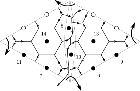
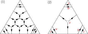
Moreover, these coordinates are natural with respect to the action of the mapping class group of the surface . More precisely, if a different ideal triangulation is chosen, then the coordinate change map relating and is given by the tropical -coordinate cluster transformation of [FZ02, FG06], expressed locally as in Equations (1)-(5); see Figure 2.
In particular, Goncharov-Shen used the Knutson-Tao rhombus inequalities associated to an ideal triangulation of to index the set of positive tropical integer points, which they showed parametrizes a linear basis for the algebra of regular functions ; see [GS15, §3.1 and Theorem 10.12 (stated for more general Lie groups)]. Their parametrization is not mapping class group equivariant; see the remark in [GS15, page 614] immediately after the aforementioned theorem. In [GS19] they construct equivariant bases using the abstract machinery of [GHKK18]. Theorem 1.1 provides a concrete model indexing the set of positive tropical integer points, also based on the Knutson-Tao inequalities, which in addition is equivariant with respect to the action of the mapping class group. This natural indexing provided by Theorem 1.1 generalizes the case [GS15, Theorem 10.15].
We think of the web coordinates of Theorem 1.1 as positive tropical integer -coordinates. We call the positive integer cone the Knutson-Tao-Goncharov-Shen cone with respect to the ideal triangulation of .
These tropical web coordinates were constructed for some simple examples, such as the eight triangle webs shown in Figure 11 below, in [Xie13]. They also appeared implicitly in [SWZ20, Theorem 8.22], in the geometric context of eruption flows on the -Hitchin component (). Xie [Xie13] checked the mapping class group equivariance, in the above sense, of these coordinates on a handful of examples.
Frohman-Sikora [FS22] independently constructed nonnegative integer coordinates for the set of reduced 3-webs. Their coordinates are related to, but different than, the coordinates of Theorem 1.1.
As an application, Kim [Kim20] constructed an explicit -version of Fock-Goncharov duality using the tropical web coordinates of Theorem 1.1, in the setting of non-marked surfaces . We expect that Kim’s approach, together with the -quantum trace map [Dou21, Kim20], will lead to an explicit -version of quantum Fock-Goncharov duality [FG09]; see [AK17] for the case.
As another application, Ishibashi-Kano [IK22] generalized the coordinates of Theorem 1.1 to an -version of shearing coordinates for (unbounded) 3-laminations.
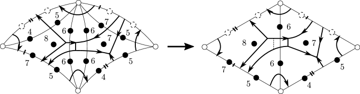
To end this subsection, we briefly recall from [DS20] the construction of the coordinate map from Theorem 1.1; see §3. Given the ideal triangulation , form the split ideal triangulation by replacing each edge of with two parallel edges and ; in other words, fatten each edge into a bigon. One then puts a given reduced -web into good position with respect to the split ideal triangulation . The result is that most of the complexity of the -web is pushed into the bigons (Figure 8), whereas over each triangle there is only a single (possibly empty) honeycomb together with finitely many arcs lying on the corners (Figure 9). Once the 3-web is in good position, its coordinates are readily computed. For an example in the once punctured torus, see Figure 1.
1.2. Local aspects
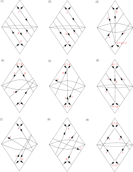
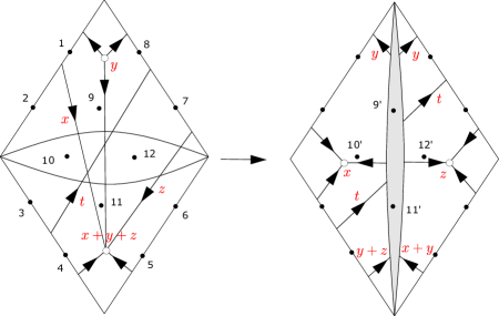
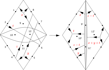
The first new contribution of the present work is a proof of the naturality statement appearing in Theorem 1.1; see §4. This is a completely local statement, since any two ideal triangulations and are related by a sequence of diagonal flips inside ideal squares. It therefore suffices to check the desired tropical coordinate change formulas for a single square:
| (1) |
| (2) |
| (3) |
| (4) |
| (5) |
See Figure 2 for the notation.

Given a -web in good position with respect to , the restriction of to a triangulated ideal square falls into one of 42 families for . Depending on which family the restricted web belongs to, there is an explicit topological description of how rearranges itself into good position after the flip; see §5. These local 42 families of -webs in the square have a geometric interpretation, leading to our second main result.
Let be a disk with four marked points, namely an ideal square, and let be a choice of diagonal of . Theorem 1.1 says that the set of reduced -webs in embeds via as a positive integer cone inside . This cone possesses a finite subset of irreducible elements spanning it over , called its Hilbert basis [Hil90, Sch81]; see §6.
Theorem 1.2.
The Knutson-Tao-Goncharov-Shen cone associated to the triangulated ideal square has a Hilbert basis consisting of elements, corresponding via to reduced -webs for .
Moreover, the positive integer cone
can be decomposed into sectors : (I) each sector is generated over by of the Hilbert basis elements, and (II) adjacent sectors are separated by a codimension wall. These sectors are in one-to-one correspondence with the families of -webs in the square, discussed above.
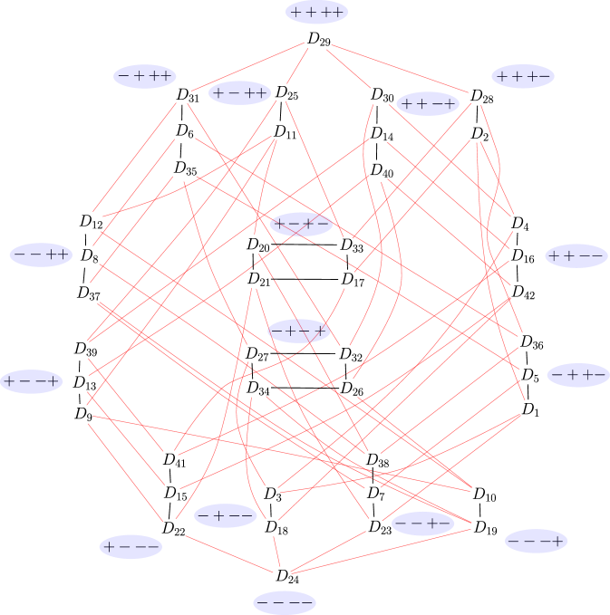
Lastly, each family contains distinguished -webs for , corresponding to the Hilbert basis elements generating the sector . We refer to the set of these distinguished -webs as the topological type of the sector . Then, two sectors and are adjacent if and only if their topological types differ by exactly one distinguished -web; see Figure 3.
We like to think of Theorem 1.2 as expressing a topological wall-crossing phenomenon. Investigating whether it could be related to other wall-crossing phenomena appearing in cluster geometry [KS08] might be an interesting problem for future research.
For a related appearance of Hilbert bases, in the setting, see [AF17].
The proof of Theorem 1.2 is geometric in nature and might be of independent interest. Recall [FG06] there are two dual sets of coordinates for the two dual moduli spaces of interest, respectively, the -coordinates and the -coordinates, as well as their tropical counterparts. For a triangulated ideal square , via the mapping each -web is assigned 12 positive tropical integer -coordinates . We show that there are also assigned to four internal tropical integer -coordinates valued in , two associated to the unique internal edge of and one for each triangle of ; see Figure 24 below. We find that the decomposition of the -cone into 42 sectors is mirrored by a corresponding decomposition of the -lattice into 42 sectors; see Figure 3. We think of this as a manifestation of Fock-Goncharov’s tropicalized canonical map:
The image of the map is , and maps sectors of the positive integer cone to sectors of the integer lattice . See §7.
Acknowledgements
We are profoundly grateful to Dylan Allegretti, Francis Bonahon, Charlie Frohman, Sasha Goncharov, Linhui Shen, Daping Weng, Tommaso Cremaschi, and Subhadip Dey for many very helpful conversations and for generously offering their time as this project developed.
Much of this work was completed during very enjoyable visits to Tsinghua University in Beijing, supported by a GEAR graduate internship grant, and the University of Southern California in Los Angeles. We would like to take this opportunity to extend our enormous gratitude to these institutions for their warm hospitality (and tasty dinners!).
2. Background on Fock-Goncharov-Shen theory and tropical points
In this section, we recall some theoretical preliminaries in order to discuss the set of positive tropical integer -points, including the Fock-Goncharov -moduli space and the Goncharov-Shen potential.
2.1. Marked surfaces, ideal triangulations, and rhombi
A marked surface is a pair where is a compact oriented finite-type surface with at least one boundary component, and is a finite set of marked points on . Let be the set of punctures, defined as the subset of boundary components without marked points; as is common in the literature, for the remainder of the article we identify such unmarked boundary components in with the (actual) punctures obtained by removing them and shrinking the resulting hole down to a point.
We assume the Euler characteristic condition , where is the number of components of limiting to a marked point. (For example, for a once punctured disk with three marked points on its boundary.) This topological condition is equivalent to the existence of an ideal triangulation of , namely a triangulation whose set of vertices is equal to ; the vertices of are called ideal vertices.
For simplicity, we always assume that does not contain any self-folded triangles. That is, we assume each triangle of has three distinct sides. (Our results should generalize, essentially without change, to allow for self-folded triangles.)
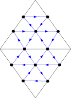
Given an ideal triangulation of , we define the ideal -triangulation of to be the triangulation of obtained by subdividing each ideal triangle of into triangles; see Figure 4 below. The 3-triangulation has as many ideal vertices as , and has non-ideal vertices, where is defined in Notation 2.1 below.
A pointed ideal triangle is a triangle in an ideal triangulation together with a preferred ideal vertex; is called a pointed ideal 3-triangle when subdivided as part of the associated 3-triangulation .
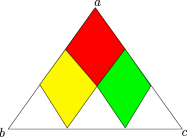
Given a pointed ideal 3-triangle, we may talk about the three associated rhombi; see Figure 5 below. In the figure, the red rhombus is called the corner rhombus, and the yellow and green rhombi are called the interior rhombi. Each rhombus has two acute vertices and two obtuse vertices. Note that exactly one of these eight vertices, the corner vertex, is an ideal vertex of ; specifically, the top (acute) vertex of the corner rhombus. (We will see below that the other vertices correspond to Fock-Goncharov -coordinates.)
Notation 2.1.
-
(1)
The natural number is defined as twice the total number of edges (including boundary edges) of plus the number of triangles of . (Note that is what we called in §1.)
-
(2)
It will be convenient to denote the nonnegative real numbers by and the nonnegative integers by . Similarly, put and .
2.2. -decorated local systems
Although not strictly required for the main theorems of the article, the material of this section and the following one §2.3 is intended to emphasize the important conceptual concepts guiding the rest of the paper.
Let be a 3-dimensional vector space.
2.2.1. -coordinates
Definition 2.2 (Decorated flags).
A flag in is a maximal filtration of vector subspaces of ,
denoted by .
A decorated flag is a pair consisting of a flag and a collection of nonzero vectors
The collection of decorated flags is denoted by .
We can think of as a homogeneous set as follows. Let be the general linear group, and let be the special linear group consisting of transformations with determinant 1. The group acts transitively on by left translation. Then can be identified with the quotient set for any maximal unipotent subgroup of (that is, in some basis of , we have that consists of upper triangular matrices with 1’s on the main diagonal, namely unipotent matrices).
We fix a volume form on . Then, a decorated flag determines a unique element satisfying the property that for all , , such that . A basis for with respect to the volume form is a choice of such a basis for the vector space .
Definition 2.3 (-moduli space [FG06, §2]).
Fix a base point in , which henceforth will be suppressed in the notation. Let be an oriented peripheral closed curve around a puncture . A decorated -local system on is a pair consisting of
-
•
a surface group representation with unipotent monodromy along each peripheral curve ; and,
-
•
a flag map , such that each peripheral monodromy fixes the decorated flag . Note that the decorated flags assigned to the marked points can be chosen arbitrarily.
Two decorated -local systems are equivalent if and only if there exists some such that and . We denote the moduli space of equivalence classes of decorated -local systems on by .
Remark 2.4.
More precisely, the flag map should be defined equivariantly at the level of the universal cover , and satisfy certain genericity conditions. These technicalities will be suppressed throughout our discussion.
Notation 2.5.
Let (resp. ) be the set of vertices of (resp. ). Note that .
We adopt the following vertex labelling conventions:
-
•
We denote a vertex on an oriented ideal edge of by , where or is the least number of edges of from to (see Figure 4).
-
•
We denote a vertex on a triangle oriented counterclockwise by , where the three nonnegative integers summing to are the least number of edges of from to , from to , and from to , respectively, where , , denote the unoriented edges of (see Figure 4).
Definition 2.6 (-coordinates [FG06, §9]).
Fix an ideal triangulation of and its -triangulation . Consider a vertex contained in a counterclockwise oriented ideal triangle , as in Figure 5. In the sense described above, choose bases, with respect to the fixed volume form ,
for the generic decorated flags , , . For a decorated local system , the Fock-Goncharov -coordinate at is
| (6) |
where , , etc. Note that this is independent of the choice of bases.
We also put , which follows from the definition of the basis of with respect to . Similarly . See also §2.3 below.
Given a quiver defined, as in Figure 4, with respect to the orientation of the surface, let
The Fock–Goncharov -coordinate at (defined for any , ) is
2.2.2. Goncharov-Shen potential
Definition 2.8 (Goncharov–Shen potential).
Let
Suppose the pointed ideal triangle (§2.1) is counterclockwise oriented, as in Figure 5. For , the monomials
| (7) |
introduced in [GS15, Lemma 3.1], correspond to the three rhombi in Figure 5. Define
Let be the collection of counterclockwise oriented pointed ideal triangles of . The Goncharov–Shen potential is
Thus, for a given ideal triangulation , the Goncharov-Shen potential is a positive Laurent polynomial in the -coordinates for .
Remark 2.9.
The Goncharov-Shen potential is mapping class group equivariant; in particular, it defines a rational positive function on the moduli space . In [GS15] and [GHKK18], the GS potentials are understood as the mirror Landau-Ginzburg potentials. In [HS19, §4], the GS potentials are understood as generalized horocycle lengths.
2.2.3. Tropical points
The moduli space is a positive space (Remark 2.7), so its points are defined over any semifield . To each ideal triangulation there is associated a -chart , determined by the -coordinates (§2.2.1), for the moduli space over . In this paper, we will always be working in a -chart (see Definition 2.11 below).
The higher decorated Teichmüller space is the set of positive real points of . By Remark 2.7, the cluster transformation between two triangulations and sends positive coordinates to positive coordinates. Hence, all the -coordinates of for any ideal triangulation are positive.
The tropical semifield is defined by and . The isomorphism sends to . In this section, we use . The tropical semifields and are defined in the same way.
For the tropical semifield , the -chart is identified with . Here, is the number of -coordinates, recalling Notation 2.1. Similarly, for the tropical semifields the -charts and are identified with the lattices and , respectively.
The tropical -coordinates are denoted for ; compare Definition 2.6.
The tropicalization of a positive Laurent polynomial is
Tropicalizing the Goncharov-Shen potential (§2.2.2), we have, by (7),
| (8) |
and
That is, the minimum is taken over all rhombi in all pointed ideal triangles of .
Note that, since is constant (by the discussion after (6)), we have .
Definition 2.10.
The space of positive real tropical points is
Alternatively, in -charts,
The spaces and are defined in the same way.
2.3. -decorated local systems
We are interested in a closely related moduli space defined similarly to . As we will see, the -coordinates do not make sense for . Nevertheless, the Goncharov-Shen potential is still well-defined. Following [GS15] (see the paragraph immediately following their Theorem 10.15), we can say that is a positive space, so we can talk about its points over a semifield . In particular, we can talk about its positive tropical integer points , which is our main object of study.
To define the space it suffices to say what is the set of -decorated flags, denoted by (compare Definition 2.2); the rest of the definition then mimics that of . Let be the set of quadruples where is a complete flag in and is a nonzero element of for . Then acts transitively on in the obvious way. If we view as the nonzero scalar matrices in , then acts on as well. We put . The action of descends to a transitive action of on . If is any maximal unipotent subgroup of (see §2.2.1), let also denote its quotient in . We can then view as a homogeneous set.
We denote elements of the resulting moduli space by where and (compare Definition 2.3).
By a basis of a -decorated flag we mean a linear basis of adapted to the flag and representing this projective class; that is, such that there exists some nonzero scalar so that for all .
The Goncharov-Shen potential is defined on the moduli space as follows (compare §2.2.2). Make an arbitrary choice of a volume form on , as well as a basis of the -decorated flag for each marked point or puncture . With respect to these choices, define numbers by (6), and define the rhombus numbers by (7); note that now need not be equal to . While the numbers depend on the choices we have made, one checks that the rhombus numbers do not. Thus, the potential is well-defined on .
We now turn to the tropical integer -points defined with respect to the Goncharov-Shen potential . Note . More precisely:
Definition 2.11.
Let be an ideal triangulation of . In -charts (§2.2.3), we have the following notions.
The set of lamination-tropical points is
Note this satisfies
Similarly, the set of web-tropical points is
Note, by Definition 2.10, this satisfies
We see then that we have the identities of tropical real points: and .
From now on, we always view and .
Remark 2.12.
-
(1)
It turns out (see [DS20, Remark 44]) that, in the expressions for and in Definition 2.11, we just as well could have assumed . That is, all real solutions are, in fact, one third integer solutions. Moreover, in the case of , these one third integer solutions are nonpositive (this is because the rhombus numbers (8) are opposite in sign to those appearing in [DS20]).
-
(2)
The set of lamination-tropical points was called the set of balanced points in [Kim20].
- (3)
- (4)
3. Tropical points and webs
We now introduce the main object of study, the Knutson-Tao-Goncharov-Shen cone associated to an ideal triangulation of a marked surface , and we summarize the work of [DS20] relating tropical points to topological objects called webs.
3.1. The Knutson-Tao-Goncharov-Shen cone and reduced webs
We recall only the topological and notational definitions of §2.1. Let be a marked surface.
3.1.1. KTGS cone
Given a pointed ideal triangle in an ideal triangulation of (§2.1), assume nonnegative integers (see also Remark 2.12(1)) (resp. ) are assigned to some interior (resp. corner) rhombus, where the numbers are assigned to the two obtuse vertices, and the numbers are assigned to the two acute vertices. To such an assigned rhombus, we associate a Knutson-Tao rhombus inequality and a modulo 3 congruence condition . Here, we set if the rhombus is a corner rhombus, where then corresponds to the corner vertex.
Definition 3.1.
A positive integer cone is a submonoid of (Notation 2.1) for some . That is, is closed under addition and contains the zero vector.
Recall the definition (Notation 2.1) of the natural number . This is the same as the number of non-ideal points of the 3-triangulation . We order these non-ideal points arbitrarily in the following definition (compare §4.3), so that to each such non-ideal point of we associate a coordinate of . In this way, a point of assigns to each rhombus in a pointed ideal triangle four numbers as above.
Definition 3.2.
Given an ideal triangulation of , let the Knutson-Tao-Goncharov-Shen cone , or just the KTGS cone for short, be the submonoid defined by the property that its points satisfy all of the Knutson-Tao rhombus inequalities and modulo 3 congruence conditions, varying over all rhombi of all pointed ideal triangles of .
Proposition 3.3.
The KTGS cone is a positive integer cone.
3.1.2. Reduced webs
A web (possibly with boundary) in [DS20, §8.1] is an oriented trivalent graph embedded in such that:
-
•
the boundary of the web lies on the boundary of the surface (minus the marked points) and may be nonempty, in which case its boundary points are required to be monovalent vertices;
-
•
the three edges of at an internal vertex are either all oriented in or all oriented out;
-
•
we allow that have components homeomorphic to the circle, called loops, which do not contain any vertices;
-
•
we allow that have components homeomorphic to the closed interval, called arcs, which have exactly two vertices on and do not have any internal vertices.
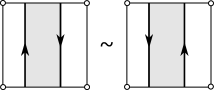
Webs are considered up to parallel equivalence, meaning related either by an ambient isotopy of or a homotopy in exchanging two “parallel” loop (resp. arc) components of bounding an embedded annulus (resp. rectangle, two of whose sides are contained in , as in Figure 6).
A face of a web [DS20, §8.1] is a contractible component of the complement . Internal (resp. external) faces are those not intersecting (resp. intersecting) the boundary . A face with sides (counted with multiplicity, and including sides on the boundary ) is called a -face. Internal faces always have an even number of sides. An external H-4-face is an external 4-face limiting to a single component of (there is only one type of external 2- or 3-face).
3.2. Web tropical coordinate map
In [DS20, §8.2], for any marked surface and for each ideal triangulation of , we defined a bijection of sets
from the set of parallel equivalence classes of reduced webs to the KTGS cone , called the web tropical coordinate map. We now recall the definition of this map.
3.2.1. Split ideal triangulations, good positions, and web schematics
The split ideal triangulation associated to , which by abuse of notation we also denote by , is defined by splitting each ideal edge of (including boundary edges) into two disjoint ideal edges. In particular, the surface is cut into ideal triangles and bigons, as shown in Figure 7. Note that although bigons do not admit ideal triangulations (in particular, they do not satisfy the hypothesis of §2.1 since ), we can still consider them as marked surfaces, where all the definitions for webs make sense.

As proved in [FS22] and [DS20, §8.2], by isotopy we can put any reduced web into good position with respect to the split ideal triangulation , meaning (see below for more details):

More precisely, the triangle condition (called “rung-less essential” in [DS20, §3.4]) is equivalent to saying that the restriction of to the triangle is reduced. The bigon condition (called “essential” in [DS20, §3.4]) is equivalent to asking that (1) all internal faces have at least six sides; and (2) for each edge of the bigon, and for every compact embedded arc in the bigon such that and such that intersects transversely, we have that the number of intersection points does not exceed the number of intersection points ; here, is the segment in between the two endpoints of . Note this is a weaker condition than being reduced, since, although it does not allow for external 2- or 3-faces, it does allow for external H-4-faces (also called “rungs” of the ladder web).
In particular, has minimal geometric intersection with the split ideal triangulation .
Note that for a web in good position: there are two types of honeycombs in triangles, out- and in-honeycombs (see Figure 9); there may or may not be a honeycomb in a given triangle; and, no conditions on the orientations of the corner arcs in a triangle are assumed.
Remark 3.5.
For an earlier appearance of these honeycomb webs in ideal triangles, see [Kup96, pp. 140-141].
In Figure 8(2) we show the bigon schematic diagram for a ladder web in a bigon, where each “H” is replaced by a crossing.
In Figure 9(2) we show the triangle schematic diagram for a honeycomb web in a triangle. Here, the honeycomb component is completely determined by two pieces of information: its orientation (either all in or all out) and a nonnegative integer . Note that the schematic for corner arcs is not a “faithful” diagrammatic representation, in general, because it forgets the ordering of the oriented arcs on each corner; see Remark 3.6. However, as we will see, this schematic is sufficient to recover the web tropical coordinates.
Remark 3.6.
As one last note about the schematic for corner arcs, if the surface is an ideal polygon (a disk with marked points on its boundary), then the schematic is indeed faithful at the level of parallel equivalence classes of reduced webs. This is because, in this setting, permuting corner arcs preserves the equivalence class of the web; see §3.1. See Figure 6, showing a boundary parallel move in the ideal square.
Definition 3.7.
Given the split ideal triangulation as in Figure 10, suppose we are given two oriented arcs intersecting in the bigon along the ideal edge between the two triangles. The intersection is called a
The following fact is essentially by definition.
Observation 3.8.
For any reduced web in good position with respect to the split ideal triangulation , the schematic diagram (Figure 8(2)) of any ladder web obtained by restricting to a bigon has only admissible crossings.
3.2.2. Definition of the web tropical coordinates

Another way to think of an ideal triangle is as an ideal polygon (Remark 3.6) with three marked points on its boundary, labeled counterclockwise say.
Let a reduced web be in good position with respect to a split ideal triangulation of . We start by defining the web tropical coordinates “locally” for each restriction of to an ideal triangle of , as in Figure 9(1).
First, the images in under of the eight “irreducible” (see §6 below) local reduced webs displayed in Figure 11 are defined as in that figure. One checks directly that these images satisfy the Knutson-Tao rhombus inequalities and the modulo 3 congruence conditions (§3.1).
Then, the image under of the restriction is defined as follows. Let be the oriented honeycomb appearing in . Let the nonnegative integers be defined by the schematic for , as in Figure 9(2). Put
Lastly, the web tropical coordinates for are defined by “gluing together” the local coordinates ) for the triangles across the edges of . Note that the pair of coordinates of along an edge at the bigon interface between two triangles and matches the corresponding pair of coordinates of along the other bigon edge , since these coordinates depend only on the number of oriented in- and out-strands crossing the bigon at either boundary edge or . Thus, this gluing procedure is well-defined. In particular, in this way coordinates are assigned to the un-split ideal triangulation ; this is why, in practice, one can go back and forth between the split and un-split triangulation.
See Figure 12 for an example where is the once punctured torus. As another example, the face coordinate (namely, the coordinate that is 3 for and ) for the honeycomb web shown in Figure 9(1) is . There are plenty of examples of computing web coordinates throughout the paper; for instance, see §5.
In [DS20, §8.2] we showed is independent of the choice of good position of with respect to the split ideal triangulation . Moreover, we proved the result mentioned at the beginning of this subsection:
Theorem 3.9 ([DS20, Theorem 80]).
For each ideal triangulation of the marked surface , the web tropical coordinate map
from the set of parallel equivalence classes of reduced webs in to the Knutson-Tao-Goncharov-Shen cone , is a bijection of sets.
We will need the following fact, which is immediate from the definitions.
Observation 3.10.
For any disjoint reduced webs , we have and
4. Naturality of the web tropical coordinates
In §3, we recalled the construction [DS20] of the web tropical coordinate map , depending on a choice of ideal triangulation of the marked surface . By Theorem 3.9, is a bijection.
In this section, we show that these coordinates are natural with respect to changing the triangulation . That is, the induced coordinate change map is a tropical -coordinate cluster transformation, in the language of Fock-Goncharov [FG06].
4.1. Precise statement of naturality for the square
Recall that an ideal square is a disk with four marked points on its boundary. (See also Remark 3.6.) An ideal triangulation of is a choice of diagonal of the square; there are two such triangulations, related by a diagonal flip.
Definition 4.2.
Let and be the two ideal triangulations of the square . The tropical -coordinate cluster transformation for the square is the piecewise-linear function
defined by
where the right hand side of the equation is given by Equations (1), (2), (3), (4), (5). See also Figure 2. (Here, we think of the domain of as associated to , and the codomain to .)
The main result of this paper is:
Theorem 4.3.
Let and be the two ideal triangulations of the square , and let and be the associated web tropical coordinate maps. Then,
Remark 4.4.
Note it is not even clear, a priori, from the definitions that for .
4.2. Proof of Theorem 4.3
By definition of the tropical coordinates, and of good position of a reduced web in with respect to the triangulations and , we immediately get:
Observation 4.5.
For all , the images and satisfy Equation (1).
Definition 4.6.
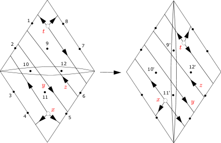
Let the punctures of the square be labeled , , , as in Figure 23 (part 1) below. Also as in the figure, define the 8 oriented corner arcs in . Their 12 coordinates are provided in the figure as well.
One checks by direct computation that:
Observation 4.7.
The images , for any of the corner arcs, satisfy Theorem 4.3.
Definition 4.8.
A given reduced web in is the disjoint union of (i) all its corner arc components, together called the corner part and denoted ; and (ii) their complement , which we call the cornerless part of the web .
A reduced web is cornerless if . That is, has no corner arcs.
Let be the set of corner webs, that is, webs whose cornerless parts are empty: . That is, an element of is a disjoint union of corner arcs.
Lemma 4.9.
For any disjoint reduced webs and , we have and
Proof.
Proof of Theorem 4.3.
Recall by Theorem 3.9 that any is of the form for some . For any reduced web , suppose that its coordinates via are labeled as in the left hand side of Figure 2, and via as in the right hand side of Figure 2. By Observation 4.5, Equation (1) is satisfied for any web in . In addition, by Observation 4.7, the Equations (2), (3), (4), (5) are satisfied for any web in , that is, consisting only of corner arcs. By Lemma 4.9 together with another application of Observation 3.10 to , we have thus reduced the problem to establishing Equations (2), (3), (4), (5) for any cornerless web .
The main difficulty is that, for a given cornerless web in good position with respect to the ideal triangulation , after flipping the diagonal it is not obvious how rearranges itself back into good position with respect to the new triangulation . (See, however, §5 for examples of this rearranging into good position after the flip.)
We circumvent this difficulty by solving the problem “uniformly”, that is, without knowing how the new good position looks after the flip. The hypothesis that the web does not have any corner arcs will be important here.
To start, observe that it suffices to establish just Equation (2). Indeed, Equations (3), (4), (5) then immediately follow by 90 degree rotational symmetry. (Solve for and , respectively, in the last two equations.)
With this goal in mind, we argue
| () |

Let us justify the first equation of ( ‣ 4.2). There are two cases, namely when represents an out- or an in-honeycomb.
When is “out”, we compute:
When is “in”, we compute:
In both cases, the desired formula holds.
The justification of the third equation of ( ‣ 4.2) is more involved. We begin with a topological consequence.
Claim 4.10.
Let be a cornerless reduced web in the square. Up to degree rotational symmetry of the square, there are three cases:
-
(1)
When the and honeycombs are both “out”: Then,
Moreover, if , then ; and, if , then .
(Note this is the case displayed in the left hand side of Figure 13.)
-
(2)
When the honeycomb is “out”, and the honeycomb is “in”: Then,
Moreover, if , then ; and, if , then .
-
(3)
When the and honeycombs are both “in”: Then,
Moreover, if , then ; and, if , then .

The key topological property used to prove all three statements of the claim is the following: The number of “out” strands (resp. “in” strands) along one boundary edge of the bigon, as displayed on the left hand side of Figure 13, is equal to the number of “in” strands (resp. “out” strands) along the other boundary edge of the bigon.
We prove the first statement, (1), of the claim; the proofs of the second and third statements are similar. So assume the and honeycombs are both “out”.
By the above topological property, we have the desired two identities of the statement.
For the second part of the statement: When , if were nonzero, then would have to be nonzero, since . Then would be attaching to ; see the schematic shown in the left hand side of Figure 14 (see also the caption of Figure 13). But this contradicts the hypothesis that has no corner arcs. Similarly, when ; see the right hand side of Figure 14. This establishes the claim.
Claim 4.11.
Let be a cornerless reduced web in the square. Up to degree rotational symmetry of the square, there are three cases:
-
(1)
When the and honeycombs are both “out”: Then, if and only if ; conversely, if and only if .
(Note this is the case displayed in the left hand side of Figure 13.)
-
(2)
When the honeycomb is “out”, and the honeycomb is “in”: Then, if and only if ; conversely, if and only if .
-
(3)
When the and honeycombs are both “in”: Then, if and only if ; conversely, if and only if .
We prove the first statement; the proofs of the second and third statements are similar. So assume the and honeycombs are both “out”. By Figure 13, we compute:
Thus,
By applying the two identities of part (1) of Claim 4.10, the above inequality is equivalent to as desired. Conversely, by reversing the direction of the inequality throughout the argument, we have if and only if . This establishes the claim.
We are now prepared to justify the third equation of ( ‣ 4.2), which we recall is
| () |
First, let us assume the and honeycombs are both “out”, as in the left hand side of Figure 13. The values of were computed above, and we gather
By Figure 13, there are two ways to express :
There are two cases to establish ( ‣ 4.2). In the case , we compute, using the second form of above:
For this case, by part (1) of Claim 4.11, we have . Thus, by part (1) of Claim 4.10, as desired.
In the case , we compute, using the first form of above:
For this case, by part (1) of Claim 4.11, we have . Thus, by part (1) of Claim 4.10, as desired.
This establishes ( ‣ 4.2) when both the honeycombs are “out”. When the honeycomb is “out”, and the honeycomb is “in”; or, when the and honeycombs are both “in”: By essentially the same calculation, one computes again that, in the case , then ( ‣ 4.2) is equivalent to , and in the case , then ( ‣ 4.2) is equivalent to . These are justified by parts (2) and (3), respectively, of Claims 4.11 and 4.10.
This completes the proof of the main result. ∎
Remark 4.12.
We emphasize that the above proof depended crucially on two topological properties (both used in the proof of Claim 4.10): (1) the bigon property about “in” and “out” strands; and, (2) the cornerless property saying that and cannot be simultaneously nonzero.
The trick was to use Lemma 4.9 to separate the corner arc case from the cornerless case, and then to use the fact that it is obvious that the boundary coordinates do not change after the flip. It is somewhat surprising that there is this relationship ( ‣ 4.2) between the internal and boundary coordinates; we do not know if such a relationship occurs in higher rank. In §7, we give another application of this “separating corner and cornerless webs” strategy.
4.3. Naturality for a marked surface
Let be a marked surface, let be an ideal triangulation, and let denote the number of global tropical coordinates; see §2.1. In §3, we introduced the web tropical coordinate map , where we implicitly assumed an inclusion of the KTGS cone of (any permutation of the coordinates of determines a different inclusion). This choice played no role there, since we were only considering a single triangulation. We now consider multiple triangulations, where it becomes necessary to keep track of such choices.
4.3.1. Dotted triangulations
More precisely, let be an initial choice of ideal triangulation, which we mark with dots in the usual way (as for instance in Figure 4). Such a dotted initial triangulation is called a base (dotted) triangulation. Fix a labeling of the dots of from ; we say that the base triangulation is labeled. This determines a bijection , hence also an inclusion (since a point in is, most precisely, a function ; see Figure 11 for instance).
Example (part 1).
See the first diagram 0 in Figure 15.
We now imagine forgetting , but leaving the dots associated to where they were on the surface. Another triangulation is dotted (with respect to the dotting of ) if there are two dots (from ) on each edge of and one dot (from ) in each face of . Note that, using the labeling of the dots fixed along with the base triangulation , each dotted triangulation determines an inclusion as above for .
We refer to without a dotting as the underlying topological triangulation.
Example (part 2).
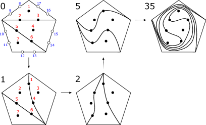
The triangulations , , , shown in the last four diagrams 1, 2, 5, 35 in Figure 15 are dotted with respect to the dotted triangulation in the first diagram 0. Note that, as triangulations, , but, as dotted triangulations, .
4.3.2. Tropical -coordinate cluster transformation for a marked surface
We pause our discussion of the topology and geometry of webs and cones, and turn to a purely algebraic result of Fomin-Zelevinsky and Fock-Goncharov (see Theorem 4.13 below).
There is a procedure to start from a base triangulation and generate new dotted triangulations in a controlled way, via diagonal flips. Indeed, if is dotted, and if is a triangulated square in , the diagonal flip at induces a new dotted triangulation . (For simplicity, we always assume that is not self-folded; see §2.1.) Note that the induced embedding of in is well-defined up to isotopy in , since the triangulated square comes with a canonical foliation including the diagonal as a leaf. Observe that the sequence of dotted triangulations so-obtained depends on the chosen sequence of diagonal flips, so is not unique.
Example (part 3).
See for instance the passage from the diagrams 0 to 1 or from the diagrams 1 to 2 in Figure 15.
Let be labeled as well, and let and be as above. Then their dottings induce a flip mutation function
defined in the square as in Definition 4.2 (that is, by the formulas (1), (2), (3), (4), (5) of Figure 2) and outside the square as the identity. (We remind that the domain is associated to and the codomain to .) In particular, the formulas are the same irrespective of whether the boundary of the square has any self-gluings. If
| () |
is a sequence of flips as above, ending at a dotted triangulation , define the associated mutation function (for this sequence of flips)
as the function composition
Here, we have used the standard convention that .
Now, let in addition
| () |
be another sequence of diagonal flips starting at the same base triangulation , and ending at the same topological triangulation , but where the dottings of and are possibly different. Define the associated permutation linear map
as follows: For , if the -labeled dot is on an edge (resp. face) of , and if the corresponding dot on the corresponding edge (resp. face) of is labeled , then maps the -th standard basis vector of to the -th standard basis vector of .
Example (part 4).
We could take in Figure 15 with and . Then,
and is the identity on all of the boundary coordinates ().
An immediate consequence of this theorem is:
Observation 4.14.
Example (part 5).
To get a feel for the content of Theorem 4.13, let us consider (similar to part 4 of this example) in Figure 15 with and , where is defined by
and for .
Then Observation 4.14 says is the identity map . This is the so-called Pentagon Relation for . By construction this is obvious for the 8-th through the 17-th coordinates, because these are the “frozen” coordinates on the boundary of the pentagon. So the heart of the statement is the validity of the seven identities:
where is defined as the -th component of . In particular, is a complicated piecewise-linear function built out of the operations , , and .
Remark 4.15.
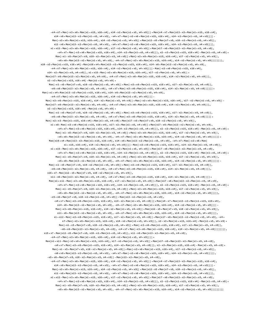
Of the seven identities discussed in Example (part 5), the most nontrivial is the case . Appendix B at the end of this article contains a Mathematica notebook which provides the explicit expression for .
To finish this digression, a well-known fact [Pen87] says that any two triangulations and are related by a sequence of diagonal flips ( ‣ 4.3.2). By Theorem 4.13, we thus immediately obtain:
Corollary 4.16.
Let be a labeled base dotted triangulation. For any topological triangulation , there is a function
defined only up to permutation of the coordinates of the codomain , satisfying the property that if is related to by a sequence of diagonal flips ( ‣ 4.3.2), then
where the are the corresponding (well-defined) flip mutation functions. ∎
Definition 4.17.
The (pseudo-)function from Corollary 4.16 is called the tropical -coordinate cluster transformation for the marked surface associated to the labeled base dotted triangulation and the topological triangulation . Below, we will drop the subscript and just write for this function.
Remark 4.18.
-
(1)
Throughout this sub-subsection, there has been nothing special about the integers compared to, say, the rational numbers . In particular, Theorem 4.13 makes sense and is true with replaced by .
- (2)
4.3.3. Naturality of the web tropical coordinate map
We are now ready to generalize Theorem 4.3 to any marked surface .
Let be a labeled base dotted triangulation, and let be any topological triangulation; see §4.3.1. Associated to this topological data is the tropical -coordinate cluster transformation , which is only defined up to permutation of the coordinates of the codomain ; see Definition 4.17.
Lastly, recall from §4.3.1 that the labels for the dots of determine an inclusion of its KTGS cone. Since is not assumed to be dotted, the inclusion of its KTGS cone is only defined up to permutation of the coordinates of .
Theorem 4.19.
Let and be triangulations, and let be the corresponding tropical -coordinate cluster transformation, as just explained. For the associated web tropical coordinate maps and , we have
where this equality is only defined up to permutation of the coordinates of .
Proof.
This is essentially an immediate consequence of Theorem 4.3.
Conceptual Remark 4.20.
Another way to express Theorem 4.19, common in the literature, is to say that the web tropical coordinates, determined by the maps , are equivariant with respect to the extended mapping class group of the marked surface . Said another way, they form natural coordinates for the positive tropical integer -points , where a point in is thought of concretely as a reduced web in .
Application 4.21.
Generalizing Fock-Goncharov’s (bounded) -laminations [FG06, §12], Kim [Kim20] considers the space of (bounded) -laminations (he denotes this space by ), which extends the space of reduced webs by allowing for negative integer weights around the peripheral loops and arcs. He also extends the web tropical coordinate map of Theorem 3.9 to an injective map , and characterizes the image as an integer lattice defined by certain balancedness conditions; it turns out that these conditions are equivalent to the modulo 3 congruence conditions of Definition 3.2. That is, whereas the reduced webs correspond to solutions of both the modulo 3 congruence conditions and the Knutson-Tao inequalities, the -laminations correspond to solutions of only the modulo 3 congruence conditions.
By [Kim20, Proposition 3.35], which generalizes Theorem 4.19, the lamination tropical coordinates are also natural, thereby constituting an explicit model for the tropical integer -points ; compare Remark 4.20 and see also Remark 2.12(2).
Kim’s proof of [Kim20, Proposition 3.35] uses Theorem 4.19. One way to think about upgrading the naturality statement from webs to laminations is in terms of the proof strategy of Theorem 4.3; see §4.2, in particular Remark 4.12. Indeed, since Lemma 4.9 works as well for corner arcs with integer coefficients, the proof of Theorem 4.3 works more generally for the laminations .
Application 4.22.
5. Web families and flip examples in the square
In §4, we proved the naturality of the web tropical coordinates without having to see what the new good position of a web in the square looks like after flipping the diagonal, which is topologically nontrivial. In this section, we give some examples of seeing the good position after the flip. This gives us another way to check the formulas of Theorem 4.3; see also Remark 4.1 at the beginning of §4. These topological developments (in particular, Proposition 5.1) will also be applied in §7 in order to study the structure of the Knutson-Tao-Goncharov-Shen cone of the triangulated square.
5.1. Web families
Recall the notion of a web schematic; see §3.2.1 and Remark 3.6. Recall also Definitions 4.6 and 4.8, for the notions of corner webs and cornerless webs .
Proposition 5.1.
We can write the reduced webs in the square as a union
of families of reduced webs, where by definition if its cornerless part can be represented by the -th cornerless schematic, of which are shown in Figure 16 below; in fact, up to rotation, reflection, and orientation-reversing symmetry (see the caption of Figure 16), every family falls into one of these cases.
Proof.
This is a direct combinatorial count, done by hand. We note that the number of possibilities is restricted by the topology of web good positions; see Observation 3.8. ∎
Notation 5.2.
Remark 5.3.
If we define an equivalence relation on the 42 families by rotation, reflection, and orientation-reversing symmetry, then (using Notation 5.2 just above):
-
(1)
The symmetry class of has four members: ; .
-
(2)
The symmetry class of has four members: ; .
-
(3)
The symmetry class of has eight members: ; .
-
(4)
The symmetry class of has eight members: ; .
-
(5)
The symmetry class of has four members: ; .
-
(6)
The symmetry class of has four members: ; .
-
(7)
The symmetry class of has four members: ; .
-
(8)
The symmetry class of has four members: ; .
-
(9)
The symmetry class of has two members: ; .
We emphasize that each schematic in Figure 16 represents a subset of reduced webs in the square. Note these subsets are not disjoint. Indeed, each intersection is at least “8-dimensional”, in an appropriate sense (see §7), since the set of corner webs is contained in each family . This intersection can contain more than just the corner webs. For instance, the intersection , corresponding to schematics (1) and (2) in Figure 16, is “11-dimensional” (thus, in Figure 3, sectors 29 and 30 are separated by a wall); the last, 12-th, dimension comes from the source or sink labeled with the weight in schematics (1) and (2). As another example, , corresponding to schematics (1) and (9) in Figure 16, is “10-dimensional” (thus, in Figure 3, sectors 29 and 33 are not separated by a wall). In fact, each family is “12-dimensional” (intuitively, this is because the square has 12 Fock-Goncharov coordinates): 8 dimensions come from the corner part , and 4 dimensions come from the cornerless part . Correspondingly, each cornerless schematic in Figure 16 has four weights .
We remind (Remark 3.6) that, in schematics (1) and (2) in Figure 16, we could have reversed the orientations of the two arc components, without changing the class of the web in . On the other hand, the orientation of the weight component distinguishes schematic (1) from (2); note the caption of Figure 16. Also by Remark 3.6, the and strands in schematic (3), for example, do not cross in the upper triangle, for otherwise the web would have an external H-4-face (§3.2.1) on the boundary.
5.2. Flip examples
The 9 symmetry classes of web families (see Figure 16 and Remark 5.3) fall into roughly three types. Let us study the flip a bit more intensively for one example of each type.
For the remainder of this section, let be a cornerless web in the square and belonging to the family , where the value of depends on which of the 9 cases we are considering (); see Notation 5.2.
Recall that (resp. ) is the triangulation shown in the left hand side (resp. right hand side) of Figure 2. Consider the web tropical coordinate maps and (see §3). Denote by
and by
compare Definition 4.2 and Figure 2. We know right away that for .
Our goal is to check that Equations (2), (3), (4), (5) are satisfied, by presenting the explicit good position of the family after the flip, allowing us to calculate the coordinates directly. We do this in the three example cases .
Recall in particular in Figure 16.
Family (1). The simplest cases are given by schematics (1) and (2) of Figure 16. We verify case (1) here. The other case is similar. We compute the ’s and ’s via Figure 11 below; see also §3.2.2.
Notice in this case it is obvious that the web on the right hand side of Figure 17 is in good position with respect to the flipped triangulation.
Left hand side of Figure 17, coordinates :
Right hand side of Figure 17, coordinates :
-
Eq. (2):
.
-
Eq. (3):
.
-
Eq. (4):
-
Eq. (5):
.
Family (3). The next simplest cases are given by schematics (3), (4), (5), (6), and (9) of Figure 16. We verify case (3) here. The other four cases are similar. We compute the ’s and ’s via Figure 11 below; see also §3.2.2.
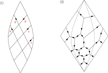
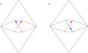
Unlike in the previous example, it is less obvious that the schematic appearing on the right hand side of Figure 18 faithfully displays how the good position looks after the flip. That this is indeed the case is a bit subtle topologically, however can be verified by an explicit procedure that draws the desired flipped bigon on top of the starting web as represented by the left hand side of Figure 18. We demonstrate this bigon drawing procedure in Figure 25 in Appendix A at the end of this article.
The schematic diagram of the web in good position restricted to the flipped bigon in the right hand side of Figure 18 is shown in Figure 19(1). It is an enjoyable exercise to check that this bigon schematic agrees with the web example schematically shown in Figure 25.
Another guiding example showing the web in good position after the flip (without using schematics), is provided in Figure 19(2).
Left hand side of Figure 18, coordinates :
Right hand side of Figure 18, coordinates :
-
Eq. (2):
.
-
Eq. (3):
.
-
Eq. (4):
.
-
Eq. (5):
.
Family (7). The last group of cases are given by schematics (7) and (8) of Figure 16. We verify case (7) here. The other case is similar. We compute the ’s and ’s via Figure 11 below; see also §3.2.2.
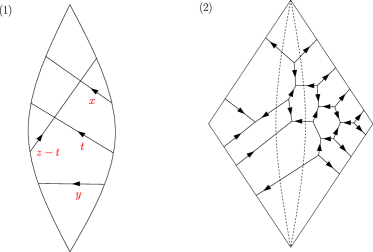
Note that, unlike for the previous two examples, in this case there are two possibilities: and . In Figure 20, we display the case when (the case is similar).
As for the previous example, it is not immediately obvious that the schematic appearing on the right hand side of Figure 20 displays the correct good position. We again verify this by explicitly drawing the flipped bigon, as shown in Figure 26 in Appendix A at the end of this article.
The schematic diagram of the web in good position restricted to the flipped bigon in the right hand side of Figure 20 is shown in Figure 21(1). It is an enjoyable exercise to check that this bigon schematic agrees with the web example schematically shown in Figure 26.
Another guiding example showing the web in good position after the flip (without using schematics), is provided in Figure 21(2).
We demonstrate the calculation when (the case is similar).
Left hand side of Figure 20, coordinates :
Right hand side of Figure 20, coordinates :
The following computations verify Equations (2), (3), (4), (5) in this case. Note that the last equation uses the assumption .
-
Eq. (2):
.
-
Eq. (3):
.
-
Eq. (4):
.
-
Eq. (5):
.
6. KTGS cone for the square: Hilbert basis
In the remaining two sections, we study the structure of the Knutson-Tao-Goncharov-Shen cone associated to an ideal triangulation of a marked surface (Definition 3.2 and Proposition 3.3) when is an ideal square. In this case, an ideal triangulation is simply a choice of a diagonal of .
6.1. Positive integer cones and Hilbert bases
Definition 6.1.
A subset (or ) is a submonoid if is closed under addition and contains 0.
Definition 6.2.
Let (or ) be a submonoid. An element is irreducible if is nonzero, and cannot be written as the sum of two nonzero elements of .
We denote by the set of irreducible elements of .
A subset is:
-
•
-spanning if every is of the form for some and , in which case we write ;
-
•
a minimum -spanning set if, in addition, for every -spanning set we have .
Note that a minimum -spanning set is unique if it exists.
Recall (Definition 3.1) that a positive integer cone is a submonoid of .
Proposition 6.3.
The subset of irreducible elements of a positive integer cone is the unique minimum -spanning subset of .
Proof.
If is irreducible and is in the -span of for , then for some by the irreducibility property. Thus is contained in any -spanning set .
It remains to show that every element of is in the -span of . We argue by induction on the sum of the coordinates of ; that is, on the quantity where . This is true if , where . So assume that is nonzero, and that is in the -span of whenever . If is irreducible, we are done. Else, with both nonzero. So and . Thus, and are in the -span of by hypothesis, so is as well. ∎
Remark 6.4.
Note that the -spanning property of in Proposition 6.3 is not true if we had only assumed that is a submonoid of . For example, the submonoid has no irreducible elements.
Definition 6.5.
Let be as in Proposition 6.3. If is a finite set, then it is called the Hilbert basis of the positive integer cone .
Example 6.6.
6.2. Hilbert basis of the KTGS cone for the triangle and the square
6.2.1. Hilbert basis for the triangle
We begin by recalling from [DS20, §5] the case of a single ideal triangle . Let be the corresponding KTGS positive integer cone.
Recall the eight “irreducible” webs in defined in §3.2.2. For each such web , its 7 tropical coordinates are provided in Figure 11.
Proposition 6.8.
The -element subset
is the Hilbert basis of the KTGS cone for the triangle.
Proof.
This is a consequence [DS20, Proposition 45] and its proof.
Indeed, we need to show that is the set of irreducible elements. To start, any such is nonzero. By the last sentence of [DS20, Proposition 45], we have that is a -spanning set for . One checks by hand that no single element of can be written as a -linear combination of other elements of . (This last property is particularly clear when viewed in the isomorphic cone , namely the image of under a certain linear isomorphism of geometric origin; for details, see the proof of [DS20, Proposition 45]. In §7, we generalize this linear isomorphism to the square case.)
The result follows by Proposition 6.3. ∎
Remark 6.9.
As a word of caution, [DS20, Proposition 45] does not imply that an element of has a unique decomposition as a sum of Hilbert basis elements. Indeed, in , we have the relation . See also §6.3 below.
It is also not true that if , in the sense that the inequality holds for each coordinate, then is topologically “contained in” . Indeed, in the above example, we have or in . An even simpler example is .
6.2.2. Hilbert basis for the square
We turn to the square , which for the rest of this section is equipped with an ideal triangulation , namely a choice of diagonal of .
Recall the 8 oriented corner arcs in the square (Definition 4.6); these are the “irreducible” webs (1)-(8) in depicted in Figure 23 (part 1). The triangulation determines 14 more “irreducible” webs in , namely the webs (9)-(22) in depicted in Figure 23 (part 2). The bracket notation used in Figure 23 (part 2) is explained in the caption of the figure. In sum, let us denote these 22 “irreducible” webs by for .
Let be the associated web tropical coordinate map. For each web , its 12 tropical coordinates are also provided in Figure 23 (part 2).
Theorem 6.10.
For the webs in displayed in Figure 23, the subset
is the Hilbert basis of the KTGS cone for the triangulated square .


Remark 6.11.
Note that if the other triangulation of had been chosen, then only the webs and would appear among the 22 “irreducible” webs corresponding to . In other words, the set of webs corresponding to the Hilbert basis of depends on which triangulation of the square is chosen.
We will need a little bit of preparation before proving the theorem.
Let and be the two triangles appearing in the split triangulation of (§3.2.1). Say, is the top triangle on the left hand side of Figure 2, and is the bottom triangle. In particular, neither nor include the intermediate bigon. If is a reduced web in in good position with respect to the split ideal triangulation , then the restrictions and are in good position in their respective triangles (by definition of good position of with respect to ). At the level of coordinates, this induces two projections and defined by and . Compare Figure 12.
Lemma 6.12.
For a reduced web in , suppose its image is an irreducible element of . Then, the projections and are, respectively, in the Hilbert bases and of the cones and .
Consequently, the set of irreducible elements of is finite (thus forming a Hilbert basis) and is a subset of , as defined in Theorem 6.10.
Proof.
Assuming the first statement, the second statement immediately follows by Definition 6.5, Proposition 6.8, and the construction of the 22 element set .
To establish the first statement, assume is in good position with respect to . It suffices to show that if is reducible, then is reducible. So assume that there are nonempty reduced webs and in such that in . (At this point, one should be mindful of Remark 6.9.) We explicitly construct nonempty reduced webs and in such that
| () |
Let (resp. ) denote the bigon edge intersecting (resp. ). Let and (resp. and for ) be, respectively, the number of out- and in-strand-ends of (resp. ) on ; similarly, let and be, respectively, the number of out- and in-strand-ends of on . Note and .
By [DS20, Definition 35, property (2)], which says that the two edge coordinates on uniquely determine the number of out- and in-strand-ends on (this is a simple linear algebra calculation), we must have and . We gather and .
Now, for each , arbitrarily choose out-strand-ends and in-strand-ends of on , which we call -strand-ends of . Let us say that a component of is -connecting if at least one of its strand-ends on is an -strand-end; note that (1) a corner arc is -connecting for at most one (possibly none, when is on the corner opposite ), and (2) a honeycomb is -connecting for at least one , and may be both - and -connecting.
Let be the size of the honeycomb of , and let be the number of -strand-ends of ; note that . For each , define to be the reduced web in consisting of the -connecting corner arc components of together with a honeycomb of size oriented as (and we can include the non--connecting components into , say); note in particular that .
Lastly, for each , define in to be the unique nonempty reduced web in the square obtained from the triangle webs and by gluing across the bigon in the usual way (as in Figure 8). (Technically, it is the class of in that is unique, and is determined up to corner arc permutations). By construction, ( ‣ 6.2.2) holds. ∎
6.2.3. Two linear isomorphisms: first isomorphism by rhombus numbers
Recall (Definition 3.2) that the KTGS cone for any triangulated marked surface is defined as the points in satisfying two conditions per rhombus, where there are three rhombi per pointed ideal triangle of (§2.1). Both conditions involve the quantity associated to the rhombus; the first being that , and the second that is an integer. (Recall if the rhombus is a corner rhombus; §2.1.) Let denote these rhombus numbers, varying over all the rhombi of .
It will be convenient in the remainder of the paper to talk about real vector spaces , which we think of as containing , in particular the KTGS cone , as a subset.
In this sub-subsection, for the triangulated ideal square we define a linear isomorphism of real 12-dimensional vector spaces, which is used in the proof of Theorem 6.10 and in §7. Here, 12 is the number of tropical coordinates for the square. Note that the triangulated square has 18 rhombi , as displayed in Figure 24 below in §7.
Definition 6.13.
Let be the triangulated square, whose coordinates are labeled as in the left hand side of Figure 2. Define a linear map
by the formula
where the are the 18 rhombus numbers defined above.
For example, the images under of the 22-element Hilbert basis of Theorem 6.10 are calculated from Figures 23 and 24 to be:
When there is no confusion, we also let denote the general -th coordinate of .
Consider the subspace defined by
| () | |||
See §7.3.1 for a discussion of the geometric meaning of the subspace and the quantities .
Proposition 6.14.
The linear map is an isomorphism of onto . That is, is injective, and the image of is equal to . In particular, is -dimensional.
Proof.
By elementary linear algebra, the above 22 images span a 12 dimensional subspace of . So is injective.
That follows from the definition of the rhombus numbers ; compare Figure 24.
That is 12-dimensional follows from a computation showing that the linear map defined by
has rank 6 (note is the kernel of ). ∎
Conceptual Remark 6.15.
Recall (§2.3) . Recall also from Remark 3.4 that we view the positive integer cone as a -chart for the positive tropical integer points .
We think of as the coordinate chart of associated to the ideal triangulation , with one tropical -coordinate per dot of (§2.2).
We view the rhombus numbers as the tropicalizations of the rhombus functions on the moduli space (§2.3).
By Proposition 6.14, we can also think of the rhombus numbers as coordinates for via the isomorphism , that is:
6.3. Tropical skein relations in the KTGS cone for the square
We end this section with a noteworthy observation, which will not be needed later.
We saw in Remark 6.9 that there are interesting relations even in the KTGS cone for the triangle. In fact, this is the only relation (in the sense analogous to Proposition 6.16 below). The intuitive reason there is only 1 relation for the triangle is because the Hilbert basis for has 8 elements, whereas there are only 7 Fock-Goncharov coordinates.
We now describe all of the relations in the KTGS cone for the square. Intuitively, there are 10 relations because the Hilbert basis for has 22 elements, whereas there are only 12 Fock-Goncharov coordinates.
Proposition 6.16.
The following linear relations are independent and complete among the elements of the Hilbert basis for the KTGS cone for the square:
Proof.
More precisely, what is meant by the statement of the proposition is the following. Let be the linear map
where the webs are as in Theorem 6.10. As in the proof of Proposition 6.14, each of the 10 relations above determines an element of . Let be the kernel of . The claim is that the elements form a basis of ; in particular, is 10-dimensional.
By Figure 23, one checks that the 10 relations are satisfied, so . By elementary linear algebra, the 10 elements are linearly independent. It remains to show that the linear map has rank 12, for which it suffices to show that the 22 elements span . This is true because, by the proof of Proposition 6.14, the images of these 22 elements under the linear map span the 12 dimensional subspace . ∎
Remark 6.17.
The relations of Proposition 6.16 can be viewed as tropical skein relations. Indeed, they can be “predicted” as the result of resolving the overlapping webs in the square (corresponding to a given relation in the cone) by one of the two Kuperberg skein relations [Kup96, §4, ] (one resolution per crossing in the picture). See also [Xie13].
7. KTGS cone for the square: sector decomposition
In §6, we saw that the Knutson-Tao-Goncharov-Shen cone for the triangulated square has a Hilbert basis consisting of 22 elements (Figure 23). There are many linear dependence relations in among these Hilbert basis elements; see Proposition 6.16. In this last section, we study certain linearly independent subsets of the Hilbert basis that have topological interpretations in terms of webs.
More specifically, we show that each of the 42 web families (Proposition 5.1 and Figure 16) corresponds to a 12-dimensional subcone (called a sector) generated by 12 Hilbert basis elements. Moreover, every point in the KTGS cone lies in such a sector . These sectors have a geometric description in terms of tropical integer -coordinates (Figure 24) for reduced webs , which are functions of the corresponding positive tropical integer -coordinates (Figure 12); we already encountered some of these ideas in §6.2.3.
In summary, this analysis gives us a deeper understanding of the combinatorial, geometric, and topological properties of the KTGS cone for the square; see Figure 3.
7.1. Cones over the real numbers
Recall that (resp. ) denotes the set of nonnegative (nonpositive) real numbers.
Remark 7.1.
Some of our terminology might be non-standard, adapted for the purposes of this paper; compare Remark 6.7.
7.1.1. Cones and sector decompositions
Definition 7.2.
-
•
A (real) cone is a subset of such that
for some finite set , called a generating set of .
We also write for the above equation.
-
•
The minimum number of elements of a generating set is called the rank of the cone . A generating set of minimum size is called a basis of .
-
•
The subspace defined by
is independent of the choice of generating set , and its dimension is called the dimension of the cone . Note .
-
•
A cone is a sector if .
-
•
A cone is full if .
Example 7.3.
-
(1)
is a full cone with basis . Its rank is 2, and its dimension is 1, so it is not a sector.
-
(2)
is a full cone with basis . Its rank is 3, and its dimension is 2, so it is not a sector. Here, is the -th standard basis element.
The subcone is not full and is not a sector.
-
(3)
One checks that the full cone has rank , by taking as a basis the vertices of the -dimensional simplex centered at the origin.
-
(4)
For , the cone is a sector of rank . It is full only for , namely when is the positive orthant.
Remark 7.4.
Note that if a cone has rank and if is a generating set for , there does not necessarily exist a subset that is a basis. For example, take with generating set .
Definition 7.5.
-
•
A sector decomposition of a full cone is a finite collection of subcones satisfying:
-
–
each is a full sector;
-
–
is the union of the sectors ;
-
–
For each distinct , the intersection has empty interior (namely, this intersection does not contain an open subset of ).
-
–
-
•
If and are two full cones in , then the intersection is a wall if is a cone of dimension .
Example 7.6.
- (1)
- (2)
- (3)
- (4)
Observation 7.7.
If is a sector decomposition of a full cone , and if is a wall, then there is no other pair of sectors giving this wall: if and only if .
This essentially follows since walls have codimension 1 in . We give a proof here for completeness.
Proof of Observation 7.7.
Let the dimensional subcone be generated by . Let in the dimensional cone be linearly independent from .
Let be a fixed point in the interior of , namely for some . Then there is such that
| () |
Let be the nonzero component of perpendicular to the subspace (with respect to the standard inner product, say); note is not necessarily in . By shrinking , we can arrange that ( ‣ 7.1.1) holds with replaced by ; denote the resulting subset ( ‣ 7.1.1) by . Similarly, define a subset depending on some and . By further shrinking, let us arrange that .
So far, we have not used the assumption that is the dimension of the ambient space . We now use this assumption, to note that is 1 dimensional, and that and have nonempty interiors in .
Without loss of generality, assume . If pointed in the same direction as , then by construction would have nonempty interior, violating the hypothesis that and are part of a sector decomposition of the full cone . Thus, points in the opposite direction as .
Now, assume as well; define and as above. After possibly swapping indices, we have that and (resp. and ) point in the same direction. Arguing as above, it follows that and have nonempty interiors. Therefore, and . ∎
7.1.2. Some technical statements about cones of the form
This sub-subsection can be skipped until §7.3.3.
Lemma 7.9.
Let be a cone satisfying the following properties:
-
•
for , where is the -th standard basis element of ;
-
•
, where is the natural projection.
Then, . Namely, is full.
Example (part 1).
The rank of such a cone as in Lemma 7.9 can equal the dimension or be strictly greater. For example, has rank 3, whereas has rank 2.
Proof of Lemma 7.9.
Note , so ; see Definition 7.2. The hypothesis thus implies . It follows that . ∎
Lemma 7.10.
Consider a full cone as in Lemma 7.9. Let be a finite subset of with , and let for some be a collection of index sets of constant size .
Assume in addition:
-
•
is the union of the subcones
- •
Then, the subcones are full sectors forming a sector decomposition of .
Also, the sector projects via to the sector . Moreover, for all pairwise distinct .
Example (part 2).
For as in part 1, put and . For as in part 1, put and . In both cases, put and .
Then, in both cases, and . For , we have and . For , we have and .
Lastly, , which projects by to .
Proof of Lemma 7.10.
By construction , so . To see that the reverse inclusion holds requires a little argument. Consider a general element
For , the -coordinate of is either or the -coordinate of ; without loss of generality, assume it is . Putting to be the difference of these -coordinates, we have that has the same -coordinate as and still satisfies . We then put to be the new , and reiterate this procedure for each , updating or at each step. The end result is that and as desired.
We move on to establishing that is a sector decomposition of .
To see that is a full cone, use the hypothesis that is open in , and proceed as in the proof of Lemma 7.9. By definition, has a generating set consisting of elements. Thus, , so is a sector.
That is by hypothesis.
It remains to show that has empty interior for all pairwise-distinct . Suppose otherwise, so that there is a nonempty open subset such that . Since projections are open maps, is a nonempty open subset of contained in , contradicting that is a sector decomposition. ∎
Lemma 7.11.
Let the full cone , the sector decomposition of , and the sector decomposition of be as in Lemma 7.10.
Assume in addition:
-
•
for each such that is a wall in (Definition 7.5), we have more specifically that the intersection of index sets has elements, and
Then, for any , we have that is a wall in if and only if is a wall in . In particular, if this is the case for a given , then
| () |
This furnishes a one-to-one correspondence .
Example (part 3).
For as in part 2, the sole wall in is , corresponding to the sole wall in .
As a non-example, where the hypothesis and part of the conclusion, ( ‣ 7.11), fail: In let , , , , . Put , , , . Put . Then is a wall, but and . Note that . On the other hand, , , and . Moreover, .
Proof of Lemma 7.11.
Assume first that is a wall in . By Lemma 7.10, . Thus, since is a cone, we have that is a cone. It follows that the subspace is equal to the projection under of the subspace (Definition 7.2), the latter which is dimensional by assumption. By definition of and , we have . Thus . Hence is dimensional, as desired.
Conversely, assume is a wall in . Let (resp. ) be the unique index in (resp. ). Since (resp. ) has dimension , the set of vectors (resp. ) in is linearly independent. Since by hypothesis, it follows that any expression in of the form
must imply or , respectively.
Consequently, since (in fact, this is an equality by Lemma 7.10), any expression in of the form
implies, by applying , that . We gather that the inclusion of ( ‣ 7.11) is true. Since the reverse inclusion holds by the definitions of and , we have that ( ‣ 7.11) is true. In particular, is a cone.
To finish, we show is dimensional. By the same argument as in the first paragraph of this proof, we have . Since is dimensional by hypothesis, the claim is true.
It remains to construct the desired bijection . Indeed, let be a wall in . Put to be the wall in . By Observation 7.7, the choice of such that is unique, so is well-defined. Conversely, if is a wall of in , put . Since for some by definition, we have that is a wall in . Thus, we have defined a function (note we did not need to use Observation 7.7 for this direction). It is immediate from the construction that and are inverses of each other. ∎
7.1.3. Cone completions
Definition 7.12.
Let be a submonoid (Definition 6.1) having a finite -spanning set (we say is finitely generated). Then, its completion is the corresponding real cone with the same generating set (this is independent of the choice of generating set).
By Proposition 6.3, we immediately have:
Observation 7.13.
Example 7.14.
Lemma 7.15.
Let be a finitely generated monoid. Assume there are finitely generated submonoids such that . Then, .
Proof.
The inclusion is by definition. Let be a finite generating set for . Put , where is the Euclidean length in . Then for each , there exists some such that . Indeed, writing , put where is the largest integer less than or equal to . We have that
We now argue by contradiction. Put and suppose there is . Note . Let be the natural projection onto the unit sphere. It suffices to show there exists an open ball such that and such that does not intersect . Indeed, since by hypothesis, this would contradict that there is some point of in at distance at most from a point in the ray .
Suppose such a does not exist. Then, there is a sequence in such that in . Since the subcones are finitely generated, they are closed subsets of ; thus, is closed as well. It follows that the intersection
is compact; thus, is compact as well. We gather is closed in .
Now, since the ray through any point of intersects , we have for all . It follows by the closedness of that ; in particular, the ray through intersects . But this ray cannot intersect any subcone , as is closed under scaling by and by assumption. This is a contradiction. ∎
7.2. Sector decomposition of the KTGS cone for the triangle and the square
Recall the notion of a sector decomposition of a full cone , and of a wall between two full cones; see Definition 7.5.
Definition 7.16.
7.2.1. Sector decomposition for the triangle
Let be the ideal triangle. We will use the notation of §6.2.1.
Proposition 7.17.
The completed KTGS cone is -dimensional. Putting
yields a sector decomposition of . Moreover, is a -dimensional wall, generated by the cone points corresponding to the corner arcs in .
Proof.
This is a consequence of [DS20, Proposition 45] and its proof.
Indeed, by [DS20, Proposition 45] we have that . Thus, by Lemma 7.15. Also, again by [DS20, Proposition 45] (or elementary linear algebra), the cones , , are full; in particular, and are sectors.
As mentioned in passing during the proof of Proposition 6.8, by the proof of [DS20, Proposition 45] there is a linear isomorphism satisfying:
-
•
;
-
•
sends the corner arcs points for to the first six standard basis elements of for ;
-
•
and .
It follows that has empty interior; moreover, it is a 6-dimensional wall. As these properties are preserved by isomorphisms of , we conclude the result. ∎
Corollary 7.18.
The rank (Definition 7.2) of the completed KTGS cone is .
Proof.
By Proposition 6.8, the Hilbert basis of the positive integer cone has 8 elements. It follows by Observation 7.13 that .
By Proposition 7.17, . We show there is no generating set with 7 elements.
We again work in the isomorphic cone from the proof of Proposition 7.17. Suppose is a generating set of . Let be the natural projection. Since the standard basis element is in for , and since , after possibly changing indices we can assume, for , that where is the -th standard basis element of and .
Since, by above, has a generating set where just the one generator has a negative last coordinate, it follows that any point of with a negative last coordinate has positive second, fourth, and sixth coordinates. Thus, for .
The remaining generator must therefore have a negative last coordinate. We conclude cannot be generated with . ∎
7.2.2. Sector decomposition for the square
Let be the ideal square, equipped with an ideal triangulation , namely a choice of diagonal. We will use the notation of §6.2.2. In particular, recall the 22 Hilbert basis webs in (); see Figure 23.
We define 42 subcones () of the completed KTGS cone as follows. First, define 42 web subsets (), each containing quatre Hilbert basis webs , by:
The -th web subset is moreover a subset of the -th web family (§5.1). More precisely, each of the four Hilbert basis webs is determined by the schematic picture for the web family (as in Figure 16) by putting all but one of the variables to 0 and the remaining variable to 1. Recall that the 9 specific web families denoted in Figure 16 are the families as explained in Notation 5.2.
Definition 7.19.
For , let be the set of four webs defined just above, and recall that for are the 8 corner arcs in the square.
Define the -th completed KTGS subcone as the completion
of the -th KTGS submonoid , defined by
where is the point in the KTGS positive integer cone assigned to by the web tropical coordinate map .
The set of four webs is called the topological type of the completed KTGS subcone .
By construction of the web tropical coordinate map , we can immediately say:
Observation 7.20.
For , we have .
The main result of this section is:
Theorem 7.21.
Consider the completed KTGS cone for the triangulated square ; see Definition 7.16. Then:
-
•
is -dimensional. Namely, is a full cone; see Definition 7.2.
-
•
The completed KTGS subcones are full sectors forming a sector decomposition of ; see Definition 7.5.
-
•
The intersection is a wall if and only if has elements; that is, if and only if the topological types of and differ by a single web. In this case,
() Moreover, for each web , there exists a unique index such that
that is, such that there is a web satisfying the property that the topological type of is obtained from the topological type of by swapping with . (One might think of such a swap as a web mutation.)
In particular, each sector has walls. See Figure 3.
Example 7.22.
As an example of the second paragraph of the third item of the theorem, consider , corresponding to family (1) in Figure 16. If , then corresponding to family (2) in Figure 16, and . One similarly checks that and ; that and ; and, that and .
Note that Figure 3 provides some, but not all, of this topological information; the full information is contained in the definition of the subsets above.
Question 7.23.
We will need to make some preparations before proving the theorem. In particular, we will make use of a generalization of the linear isomorphism used in the proof of Proposition 7.17.
7.3. Proof of Theorem 7.21
7.3.1. Two linear isomorphisms: second isomorphism by tropical -coordinates
In §6.2.3, to each ideal triangulation of the square we constructed a linear isomorphism . This map sends 12 real numbers , called the (real) tropical -coordinates, to their 18 rhombus numbers . There are 6 relations (see ( ‣ 6.2.3) in §6.2.3) defining the 12-dimensional subspace , which determine four real numbers , called the (real) tropical -coordinates: they are four numbers assigned to any 18-tuple in of rhombus numbers. See Figure 24. See also [Xie13].
Remark 7.24.
The tropical -coordinates originate in Fock-Goncharov theory as tropicalized double and triple ratios [FG06, FG07b], and can be thought of in the following geometric way. For , say, consider the hexagon in the top triangle in the top left square of Figure 24. There are six tropical -coordinates assigned to the vertices of this hexagon. Then is the signed sum of these coordinates, as indicated in the figure. Similarly for .
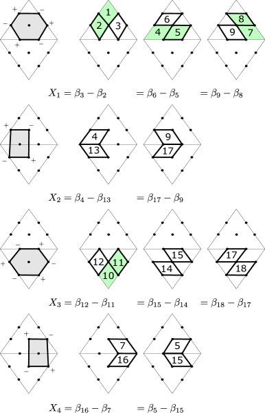
Definition 7.25.
Let be the 12-dimensional subspace just discussed. Define a linear map
by
See Figure 24, where the eight rhombi appearing in the first eight coordinates of the image of are colored green.
For example, the images under of applied to the 22 Hilbert basis elements, , can be computed from Figure 23 or from the computations in §6.2.3 to be:
Proposition 7.26.
The linear map is an isomorphism. Consequently, letting be the isomorphism from §6.2.3, we have that the composition
is a linear isomorphism.
Proof.
Since is 12-dimensional (Proposition 6.14), it suffices to show that the image of spans . Indeed, one checks by elementary linear algebra that the above 22 images span . ∎
Definition 7.27.
The linear isomorphism of Proposition 7.26 maps the completed KTGS cone to the isomorphic cone
Note that indeed lies in because is the completion of the KTGS cone , which by definition has all nonnegative (integer) rhombus numbers .
Observe, in particular, that the 8 corner arcs of Figure 23 (part 1) correspond via to the first 8 standard basis elements of .
7.3.2. Sector decomposition of via the isomorphism
Let be the cone defined in Definition 7.27, which is isomorphic, via the isomorphism , to the completed KTGS cone for the triangulated square .
Notation 7.28.
Put , , , and (compare §7.1.2).
For , define cone points by
where is the -th Hilbert basis element for the triangulated square; see Figure 23. Note that the points are displayed explicitly in §7.3.1.
For , define index sets of constant size as follows. Given , consider the topological type of the completed KTGS subcone (Definition 7.19). By definition of the topological type , there are four Hilbert basis webs , where the indices , such that . We then define the index set by
Definition 7.29.
Recalling Notation 7.28: for each , define subcones by (compare §7.1.2)
Here, is the natural projection.
Just as for the subcones , we call the topological type of the subcone .
Remark 7.30.
Note, by the calculations of §7.3.1, that the 14 vectors are distinct.
Proposition 7.31.
The subcones are full sectors forming a sector decomposition of (Definition 7.5).
Proof.
Let us begin by giving some examples of how to describe the subcones . Specifically, we will describe those 9 subcones corresponding to the topological types , which in particular are subsets of the web families displayed in Figure 16; see Notation 5.2 and Remark 5.3.
Remark 7.32.
In each of the 9 examples below, note that the ordering of the rows of the matrix does not affect the description of the subcone .
i1=29. For , let us write the four vectors in rows to form a matrix . Then for real numbers , we get
Thus .
i2=30. Similarly, for , writing the four vectors in rows, we get a matrix . Then for , we get
Thus .
i3=42. For , writing the four vectors in rows, we get a matrix . Then for , we get
Thus .
i4=17. For , writing the four vectors in rows, we get a matrix . Then for , we get
Thus .
i5=5. For , writing the four vectors in rows, we get a matrix . Then for , we get
Thus .
i6=6. For , writing the four vectors in rows, we get a matrix . Then for , we get
Thus .
i7=2. For , writing the four vectors in rows, we get a matrix . Then for , we get
Thus .
i8=1. For , writing the four vectors in rows, we get a matrix . Then for , we get
Thus .
i9=33. For , writing the four vectors in rows, we get a matrix . Then for , we get
Thus .
In the same way as the 9 examples just demonstrated, we compute directly by hand the subcones for as follows:
In particular, each subcone has dimension 4, since its explicit description via inequalities shows that it has nonempty interior in . Equivalently, one can check directly by hand that the corresponding matrix, such as in the 9 examples above, has rank 4.
Since, by Definition 7.29, the subcones are generated by 4 elements, we gather that each is a full subsector of .
One checks directly by hand that the 16 orthants decompose as:
It follows that . It remains to show that has empty interior for all pairwise-distinct . Since this is true if and lie in different orthants, we only need to check those pairs , lying in the same orthant.
This is done directly by hand; however, the cases fall into only four types. First, for orthants 1,2: There is nothing to check. Second, for orthants 3, 4, 7, 8: In 3, say, the inequalities and have codimension 1 intersection even when defined on all of , so they do as well when restricted to the orthant. The other cases go the same. Third, for orthants 15, 16: This is similar to the second type. Lastly, for orthants 5, 6, 9, 10, 11, 12, 13, 14: In 5, say, the sectors and similarly have codimension 1 intersection, as do the sectors and . This is also true for and so long as implies , which it does, since it implies whereas we are restricted to the orthant . The other cases go the same. ∎
We now analyze the walls (Definition 7.5) in the sector decomposition of . Recall (Definition 7.29) that is called the topological type of the sector .
Proposition 7.33.
The third item of Theorem 7.21 holds word-for-word, except with replaced by , and replacing ( ‣ • ‣ 7.21) by ( ‣ 7.33) below.
In particular, is a wall if and only if the intersection of their corresponding index sets has elements (see the beginning of this sub-subsection, §7.3.2). In this case,
| () |
Proof.
Any wall must, by definition, be dimensional. This restricts which indices can yield walls. Through a direct by hand check, using the explicit description by inequalities of the sector decomposition as in the proof of Proposition 7.31, one verifies that a necessary condition for to be a wall is for and to be connected by an edge in the graph depicted in Figure 3. We show this is also a sufficient condition.
More precisely, the goal is to show, for any two sectors and connected by an edge in , that has 3 elements and ( ‣ 7.33) holds. In particular, is a cone of dimension 3. Note the inclusion in ( ‣ 7.33) holds automatically; see Definition 7.29.
We checked this directly by hand. There are two types of calculations, depending on whether the sectors are in different orthants or the same orthant.
As an example where the sectors are in different orthants: We demonstrate this for and , which were computed in detail in the proof of Proposition 7.31. There, one sees that three rows of the corresponding matrix appear as rows in the matrix (recall also Remark 7.32). This means that has 3 elements; see Remark 7.30. Note that the row in that is not in corresponds to the variable , and the row in that is not in corresponds to the variable . The inclusion in ( ‣ 7.33) is true since
implies . The other different-orthant cases are similar.
As an example where the sectors are in the same orthant: We demonstrate this for and , which were also computed in detail in the proof of Proposition 7.31. There, one sees that three rows of the corresponding matrix appear as rows in the matrix (recall also Remark 7.32). This means that has 3 elements; see Remark 7.30. The row in not in corresponds to the variable , and the row in not in corresponds to the variable . The inclusion in ( ‣ 7.33) is true since
implies, by adding the third and fourth entries, that hence . The other same-orthant cases are similar.
We gather is a wall if and only if and are connected by an edge of the graph , in which case has 3 elements. In particular, since is 4-valent, the last paragraph of the third item of Theorem 7.21 holds (again, with in place of ).
To finish justifying the second paragraph of Proposition 7.33 (equivalently, the first paragraph of the third item of Theorem 7.21, appropriately substituted), we need to show that if has 3 elements (equivalently, has 3 elements), then is a wall.
So far, we have exhibited, for each , 4 topological types such that has 3 elements, all corresponding to walls . We thus need to show there are no more indices such that has 3 elements. For this, it suffices to establish the second paragraph of the third item of Theorem 7.21, which is a purely topological statement about webs in good position on the triangulated square; compare Observation 3.8 and Proposition 5.1. We checked this directly by hand; compare Example 7.22. ∎
7.3.3. Bringing everything together
We are now prepared to prove the main result of this section.
Proof of Theorem 7.21.
Let be the cone isomorphic to the completed KTGS cone via the linear isomorphism ; see Definition 7.27.
Recall also Notation 7.28 from the discussion at the beginning of §7.3.2, which should help with comparing the general lemmas of §7.1.2 to the current application.
By the explicit calculation of the Hilbert basis elements for in §7.3.1, together with Proposition 7.31, we see that satisfies the hypotheses of Lemma 7.9. Indeed, by definition, for each . Therefore, is 12 dimensional, so the isomorphic completed KTGS cone is 12 dimensional as well. This establishes the first item of Theorem 7.21.
Let us prove that ; see Definition 7.19. This follows by Theorem 3.9, Proposition 5.1, and Lemma 7.15. Indeed, by Theorem 3.9, every point in the KTGS positive integer cone is equal to for some reduced web in the square. By Proposition 5.1, the web is an element of one of the 42 web families: . By Observation 7.20, we have that . We gather that . Note that the monoid is finitely generated, since it admits a Hilbert basis (Theorem 6.10). The submonoids are also finitely generated, by Definition 7.19. We conclude by Lemma 7.15 that we have the equality of completions, as desired.
We return to the isomorphic cone . Let and be defined as in the beginning of §7.3.2. For , let the subcones be defined as in the statement of Lemma 7.10. Equivalently, the subcone is the isomorphic counterpart to the subcone . It follows by the previous paragraph that in the isomorphic cone . By this, together with another application of Proposition 7.31, we see that the hypotheses of Lemma 7.10 are satisfied. Therefore, by Lemma 7.10, we obtain the second item of Theorem 7.21, except with and replaced by and , respectively. Since this property is preserved by linear isomorphisms, we conclude the second item of Theorem 7.21 as stated.
Lastly, by Proposition 7.33, in particular ( ‣ 7.33), the hypothesis of Lemma 7.11 is satisfied. Therefore, by Lemma 7.11, the set is in one-to-one correspondence with the set in the obvious way by the projection . Moreover, a given wall can be computed by ( ‣ 7.11) in Lemma 7.11. We conclude by the remainder of Proposition 7.33 that the first and third paragraphs of the third item of Theorem 7.21 are valid, except with , , and ( ‣ • ‣ 7.21) replaced by , , and ( ‣ 7.11), respectively. Since the inverse of the linear isomorphism preserves these properties, and maps ( ‣ 7.11) to ( ‣ • ‣ 7.21) (see the beginning of §7.3.2), we conclude the first and third paragraphs of the second item of Theorem 7.21 as stated. The second paragraph is a purely topological statement about webs in the square, and was already established during the proof of Proposition 7.33. ∎
The following consequence is immediate from the proof of Theorem 7.21.
Corollary 7.34.
The function
is a surjection from the completed KTGS cone (in fact, from a “ dimensional” proper subset of ) onto . ∎
Recall the notion of a cornerless web in the square; see Definition 4.8. Let denote the set of cornerless webs up to equivalence. Note for each that .
Consider also the function defined on . See for example the nine computations at the beginning of the proof of Proposition 7.31.
Another consequence of the proof of Theorem 7.21 is:
Corollary 7.35.
The restricted function
restricted to the cornerless webs , is a surjection onto the integer lattice .
In particular, the function from Corollary 7.34 maps (a “ dimensional” proper subset of) the KTGS cone surjectively onto .
Proof.
We know that and where (Definition 7.19). We also know that the cone points in for , corresponding to the 8 corner arcs in the square, are sent by to the first 8 standard basis elements of . We gather is still a surjection onto when restricted to the subset
Note also that (similar to Observation 7.20)
It thus suffices to show: for any , if , then .
Once again, we work in the isomorphic cone , which projects to by . Put (see the beginning of §7.3.2)
and note also that
The above property is then equivalent to showing: for any such that , we have ; that is, if such a is written for (see the beginning of §7.3.2), we want to show .
This is accomplished through a direct by hand check, taking advantage of the explicit description of the sectors provided in §7.3.2. As before, although there are 42 cases, these fall into only five types, each represented among the 9 examples demonstrated in the proof of Proposition 7.31: Type 1 corresponds to ; Type 2 corresponds to ; Type 3 corresponds to ; Type 4 corresponds to ; and Type 5 corresponds to . We will only demonstrate the most nontrivial case, Type 5 (for , say); the other cases are similar.
So consider , and assume is, in addition, in for some . Note the vector is the -th row of the matrix displayed in the example in the proof of Proposition 7.31. From this example, we gather that . So ; implying by that ; implying by that , as desired. ∎
Remark 7.36.
We believe that the restricted function from Corollary 7.35 is also an injection. We suspect that there may be a proof of this result via a conjectural generalization of ( ‣ • ‣ 7.21) to higher codimension intersections.
Conceptual Remark 7.37.
We view the real cone as the isomorphic -chart .
On the other hand, via the isomorphism we view the real cone as the isomorphic -chart .
Recall, in addition to the 12 dimensional -moduli spaces and (§2), Fock-Goncharov [FG06] and Goncharov-Shen [GS15, GS19] defined the - and -moduli spaces and , which are 4- and 12-dimensional, respectively. In addition, there are canonical maps and (the overline notation may be nonstandard). The tropical points and of these spaces are also defined, inducing tropicalizations and of the canonical maps.
In terms of -charts, we view and . We think of the projection as the canonical map written in coordinates. The isomorphism could be viewed as a coordinate version of the canonical map .
We can interpret Corollary 7.34 as saying that, when expressed in coordinates, the canonical map also projects the subset of positive points onto .
References
- [AF17] N. Abdiel and C. Frohman. The localized skein algebra is Frobenius. Algebr. Geom. Topol., 17:3341–3373, 2017.
- [AK17] D. G. L. Allegretti and H. K. Kim. A duality map for quantum cluster varieties from surfaces. Adv. Math., 306:1164–1208, 2017.
- [Bul97] D. Bullock. Rings of -characters and the Kauffman bracket skein module. Comment. Math. Helv., 72:521–542, 1997.
- [CKM14] S. Cautis, J. Kamnitzer, and S. Morrison. Webs and quantum skew Howe duality. Math. Ann., 360:351–390, 2014.
- [Dou21] D. C. Douglas. Quantum traces for : the case . https://arxiv.org/abs/2101.06817, 2021.
- [DS20] D. C. Douglas and Z. Sun. Tropical Fock-Goncharov coordinates for -webs on surfaces I: construction. https://arxiv.org/abs/2011.01768, 2020.
- [FG06] V. V. Fock and A. B. Goncharov. Moduli spaces of local systems and higher Teichmüller theory. Publ. Math. Inst. Hautes Études Sci., 103:1–211, 2006.
- [FG07a] V. V. Fock and A. B. Goncharov. Dual Teichmüller and lamination spaces. Handbook of Teichmüller theory, 1:647–684, 2007.
- [FG07b] V. V. Fock and A. B. Goncharov. Moduli spaces of convex projective structures on surfaces. Adv. Math., 208:249–273, 2007.
- [FG09] V. V. Fock and A. B. Goncharov. Cluster ensembles, quantization and the dilogarithm. Ann. Sci. Éc. Norm. Supér., 42:865–930, 2009.
- [FKK13] B. Fontaine, J. Kamnitzer, and G. Kuperberg. Buildings, spiders, and geometric Satake. Compos. Math., 149:1871–1912, 2013.
- [FS22] C. Frohman and A. S. Sikora. -skein algebras and webs on surfaces. Math. Z., 300:33–56, 2022.
- [FZ02] S. Fomin and A. Zelevinsky. Cluster algebras. I. Foundations. J. Amer. Math. Soc., 15:497–529, 2002.
- [GHKK18] M. Gross, P. Hacking, S. Keel, and M. Kontsevich. Canonical bases for cluster algebras. J. Amer. Math. Soc., 31:497–608, 2018.
- [GMN13] D. Gaiotto, G. W. Moore, and A. Neitzke. Spectral networks. Ann. Henri Poincaré, 14:1643–1731, 2013.
- [GS15] A. B. Goncharov and L. Shen. Geometry of canonical bases and mirror symmetry. Invent. Math., 202:487–633, 2015.
- [GS19] A. B. Goncharov and L. Shen. Quantum geometry of moduli spaces of local systems and representation theory. https://arxiv.org/abs/1904.10491, 2019.
- [Hil90] D. Hilbert. Ueber die Theorie der algebraischen Formen. Math. Ann., 36:473–534, 1890.
- [HS19] Y. Huang and Z. Sun. McShane identities for Higher Teichmüller theory and the Goncharov-Shen potential, to appear in Mem. Amer. Math. Soc. https://arxiv.org/abs/1901.02032, 2019.
- [IK22] T. Ishibashi and S. Kano. Unbounded -laminations and their shear coordinates. https://arxiv.org/abs/2204.08947, 2022.
- [Kim20] H. K. Kim. -laminations as bases for cluster varieties for surfaces. https://arxiv.org/abs/2011.14765, 2020.
- [KS08] M. Kontsevich and Y. Soibelman. Stability structures, motivic Donaldson-Thomas invariants and cluster transformations. https://arxiv.org/abs/0811.2435, 2008.
- [KT99] A. Knutson and T. Tao. The honeycomb model of tensor products. I. Proof of the saturation conjecture. J. Amer. Math. Soc., 12:1055–1090, 1999.
- [Kup96] G. Kuperberg. Spiders for rank 2 Lie algebras. Comm. Math. Phys., 180:109–151, 1996.
- [Le16] I. Le. Higher laminations and affine buildings. Geom. Topol., 20:1673–1735, 2016.
- [MFK94] D. Mumford, J. Fogarty, and F. Kirwan. Geometric invariant theory. Third edition. Springer-Verlag, Berlin, 1994.
- [Pen87] R. C. Penner. The decorated Teichmüller space of punctured surfaces. Comm. Math. Phys., 113:299–339, 1987.
- [Prz91] J. H. Przytycki. Skein modules of 3-manifolds. Bull. Polish Acad. Sci. Math., 39:91–100, 1991.
- [PS00] J. H. Przytycki and A. S. Sikora. On skein algebras and -character varieties. Topology, 39:115–148, 2000.
- [Sch81] A. Schrijver. On total dual integrality. Linear Algebra Appl., 38:27–32, 1981.
- [Sik01] A. S. Sikora. -character varieties as spaces of graphs. Trans. Amer. Math. Soc., 353:2773–2804, 2001.
- [Sik05] A. S. Sikora. Skein theory for -quantum invariants. Algebr. Geom. Topol., 5:865–897, 2005.
- [SSW] L. Shen, Z. Sun, and D. Weng. In preparation.
- [SW07] A. S. Sikora and B. W. Westbury. Confluence theory for graphs. Algebr. Geom. Topol., 7:439–478, 2007.
- [SWZ20] Z. Sun, A. Wienhard, and T. Zhang. Flows on the -Hitchin component. Geom. Funct. Anal., 30:588–692, 2020.
- [Thu97] W. P. Thurston. Three-dimensional geometry and topology. Vol. 1. Princeton University Press, Princeton, NJ, 1997.
- [Tur89] V. G. Turaev. Algebras of loops on surfaces, algebras of knots, and quantization. In Braid group, knot theory and statistical mechanics, pages 59–95. World Sci. Publ., Teaneck, NJ, 1989.
- [Wie18] A. Wienhard. An invitation to higher Teichmüller theory. In Proceedings of the International Congress of Mathematicians—Rio de Janeiro 2018. Vol. II. Invited lectures, pages 1013–1039. World Sci. Publ., Hackensack, NJ, 2018.
- [Wit89] E. Witten. Quantum field theory and the Jones polynomial. Comm. Math. Phys., 121:351–399, 1989.
- [Xie13] D. Xie. Higher laminations, webs and N=2 line operators. https://arxiv.org/abs/1304.2390, 2013.
Appendix A Two flip examples
In Figures 25 and 26 below, we display the bigon drawing procedure, putting a web into good position after flipping the diagonal, for two examples in the web families (3) and (7), respectively, as explained in detail in §5.2.
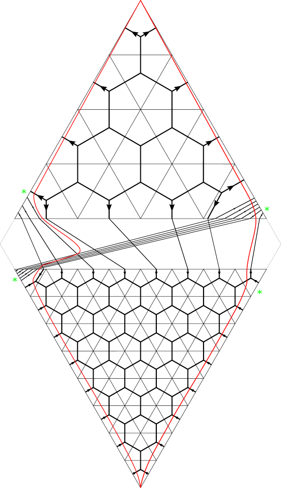
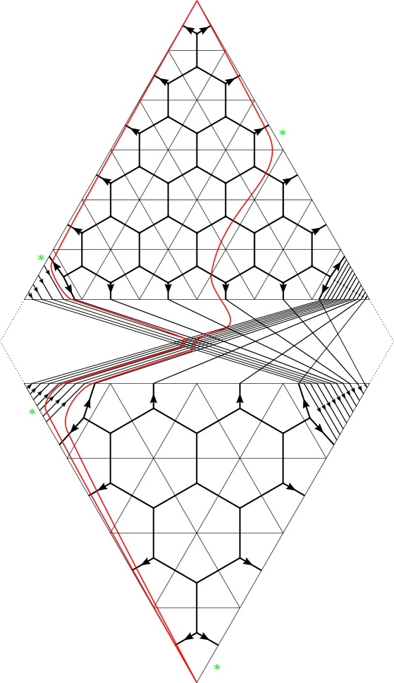
Appendix B Pentagon Relation for
The Mathematica notebook presented in Figure 28 below provides the expression for as defined in Example (part 5) from §4.3.2. See Remark 4.15.