Geometric lifting of the integrable cellular automata with periodic boundary conditions

Abstract

Inspired by G. Frieden’s recent work on the geometric $R$-matrix for affine type $A$ crystal associated with rectangular shaped Young tableaux, we propose a method to construct a novel family of discrete integrable systems which can be regarded as a geometric lifting of the generalized periodic box-ball systems. By converting the conventional usage of the matrices for defining the Lax representation of the discrete periodic Toda chain, together with a clever use of the Perron-Frobenious theorem, we give a definition of our systems. It is carried out on the space of real positive dependent variables, without regarding them to be written by subtraction-free rational functions of independent variables but nevertheless with the conserved quantities which can be tropicalized. We prove that, in this setup an equation of an analogue of the ‘carrier’ of the box-ball system for assuring its periodic boundary condition always has a unique solution. As a result, any states in our systems admit a commuting family of time evolutions associated with any rectangular shaped tableaux, in contrast to the case of corresponding generalized periodic box-ball systems where some states did not admit some of such time evolutions.

1 Introduction

1.1 Backgrounds and main results

Integrable systems in classical and quantum theory have attracted many attentions from those studying in the field of mathematical physics. Related to both classical and quantum integrable systems, the integrable cellular automata known as the box-ball systems have provided many stimulating ideas and topics in this field [8, 28]. In relation to classical integrable systems, the box-ball systems are derived from integrable non-linear differential equations by a procedure known as tropicalization or ultra-discretization. Roughly speaking, the notion of geometric lifting is the inverse of this procedure.

On the other hand, in relation to quantum integrable systems, the box-ball systems are derived from integrable quantum spin chain models by a procedure crystallization. Its mathematical background is given by Kashiwara’s theory of crystals [11, 12]. Quite remarkably, there is a geometric lifting of this theory known as the theory of geometric (and unipotent) crystals by Berenstein and Kazhdan [1]. Based on their work, G. Frieden recently presented explicit formulas for the affine type $A$ geometric crystal and its intertwiner, the geometric $R$-matrix, by using Grassmannians [2, 3]. This is a geometric lifting of the crystal of the so-called Kirillov-Reshetikhin modules and the associated combinatorial $R$-matrix, represented by semi-standard Young tableaux with rectangular shapes.

Inspired by his work, in this paper we propose a method to construct a geometric lifting of a family of integrable cellular automata with periodic boundary conditions. These cellular automata are known as the periodic box-ball system [31, 32] and its generalizations [14, 15, 16, 17]. Here we note that the periodic box-ball system was conventionally derived from time-discretized version of the closed Toda chain (or discrete periodic Toda; dp-Toda [6, 7]) by the procedure tropicalization [13, 10, 27]. Therefore one may think that its geometric lifting simply goes back to the original dp-Toda chain. However, our method of geometric lifting is considerably different from that, and gives a novel family of discrete integrable systems, which we call closed geometric crystal chains.

In order to explain the difference between the dp-Toda chain and the closed geometric crystal chain, we use the notion of discrete time Lax equation [25]. Let $\mathbf{x}=(x^{(1)},\dots,x^{(n-1)})$ be an $(n-1)$-component variable and set $x^{(n)}:=s/(x^{(1)}\cdots x^{(n-1)})$ where $s$ is a parameter in ${\mathbb{C}}^{\times}$ or ${\mathbb{R}}_{>0}$. We introduce an $n\times n$ matrix $g(\mathbf{x},s;\lambda)$ as in the main text (See Example 12 for $n=4$), in which the diagonal elements are $(x^{(1)},\dots,x^{(n)})$, their nearest lower off-diagonals are $1$’s, and there is an indeterminate $\lambda$ at the top-right corner. Then, for any $s,l\in{\mathbb{C}}^{\times}$ and sufficiently generic $(\mathbf{a},\mathbf{b})\in({\mathbb{C}}^{\times})^{2(n-1)}$, there is a unique solution $(\mathbf{a}^{\prime},\mathbf{b}^{\prime})\in({\mathbb{C}}^{\times})^{2(n-1)}$ to the following matrix equation

$$g(\mathbf{b},s;\lambda)g(\mathbf{a},l;\lambda)=g(\mathbf{a}^{\prime},l;\lambda)g(\mathbf{b}^{\prime},s;\lambda).$$ (1)

By regarding the map $T:(\mathbf{a},\mathbf{b})\mapsto(\mathbf{a}^{\prime},\mathbf{b}^{\prime})$ as a time evolution, we obtain a non-linear dynamical system on $({\mathbb{C}}^{\times})^{2(n-1)}$ which (with a shift of the indices of the variables’ components) turns out to be the dp-Toda chain. Its Lax representation is given by

$$\mathcal{L}(\mathbf{a}^{\prime},\mathbf{b}^{\prime};\lambda)=(\mathcal{M}(\lambda))^{-1}\mathcal{L}(\mathbf{a},\mathbf{b};\lambda)\mathcal{M}(\lambda),$$

where $\mathcal{L}(\mathbf{a},\mathbf{b};\lambda)=g(\mathbf{a},l;\lambda)g(\mathbf{b},s;\lambda)$ and $\mathcal{M}(\lambda)=(g(\mathbf{b},s;\lambda))^{-1}$. We note that this map is an example of what are called integrable or Yang-Baxter maps [23, 29].

For the dp-Toda chain, it is known that every component of the dependent variables $(\mathbf{a}^{\prime},\mathbf{b}^{\prime})$ is expressed by a subtraction-free rational function of the parameters $s,l$ and the components of the independent variables $(\mathbf{a},\mathbf{b})$ with non-negative integer coefficients. This implies that, if we let the parameters $s,l$ to take their values in ${\mathbb{R}}_{>0}$, then we can regard the dp-Toda chain as a dynamical system on $({\mathbb{R}}_{>0})^{2(n-1)}$ instead of $({\mathbb{C}}^{\times})^{2(n-1)}$. This idea of restricting the domains of the parameters and the variables into positive real spaces opens a door to the possibility of constructing a new family of discrete integrable systems out of this well-known matrix $g(\mathbf{x},s;\lambda)$. More precisely, we are going to adopt a new guiding principle of our study for seeking such integrable systems that have positive real dependent variables but now without regarding them to be written by subtraction-free rational functions of independent variables.

To be more explicit, one of the main results of this paper (Theorem 16) claims that for any $L\in{\mathbb{Z}}_{>0}$, $s,l\in{\mathbb{R}}_{>0}$ and $(\mathbf{b}_{1},\dots,\mathbf{b}_{L})\in({\mathbb{R}}_{>0})^{L(n-1)}$, there is a unique positive real solution $(\mathbf{v},\mathbf{b}^{\prime}_{1},\dots,\mathbf{b}^{\prime}_{L})\in({\mathbb{R}}_{>0})^{(L+1)(n-1)}$ to the following matrix equation

$$g(\mathbf{b}_{1},s;\lambda)\cdots g(\mathbf{b}_{L},s;\lambda)g(\mathbf{v},l;\lambda)=g(\mathbf{v},l;\lambda)g(\mathbf{b}^{\prime}_{1},s;\lambda)\cdots g(\mathbf{b}^{\prime}_{L},s;\lambda).$$ (2)

This remarkably simple result is obtained by combining Frieden’s work on the geometric $R$-matrix [3] with the Perron-Frobenius theorem in linear algebra (See, for example [21]). Therefore, by regarding the map $T^{(1)}_{l}:(\mathbf{b}_{1},\dots,\mathbf{b}_{L})\mapsto(\mathbf{b}^{\prime}_{1},\dots,\mathbf{b}^{\prime}_{L})$ as a time evolution, we obtain a non-linear dynamical system on $({\mathbb{R}}_{>0})^{L(n-1)}$. This is an example of the closed geometric crystal chains. Obviously, its Lax representation is given by

$$\mathcal{L}(\mathbf{b}^{\prime}_{1},\dots,\mathbf{b}^{\prime}_{L};\lambda)=(\mathcal{M}(\lambda))^{-1}\mathcal{L}(\mathbf{b}_{1},\dots,\mathbf{b}_{L};\lambda)\mathcal{M}(\lambda),$$

where $\mathcal{L}(\mathbf{b}_{1},\dots,\mathbf{b}_{L};\lambda)=g(\mathbf{b}_{1},s;\lambda)\cdots g(\mathbf{b}_{L},s;\lambda)$ and $\mathcal{M}(\lambda)=g(\mathbf{v},l;\lambda)$. Although we adopted the above mentioned guiding principle, this Lax representation allows us to obtain such conserved quantities that still can be tropicalized.

Now we want to explain how the above defined closed geometric crystal chains are related to integrable cellular automata with periodic boundary conditions. The geometric $R$-matrix (in the totally one-row tableaux case) is a map defined to be $R:(\mathbf{b},\mathbf{a})\mapsto(\mathbf{a}^{\prime},\mathbf{b}^{\prime})$ in which the variables are related by the matrix equation (1). For a state $(\mathbf{b}_{1},\dots,\mathbf{b}_{L})\in({\mathbb{R}}_{>0})^{L(n-1)}$ and a ‘carrier’ $\mathbf{v}\in({\mathbb{R}}_{>0})^{n-1}$ we use this map repeatedly. It is illustrated as

      (3)

We warn that this diagram should be read from the right to the left. So the variables are related by $R(\mathbf{b}_{i},\mathbf{v}_{i+1})=(\mathbf{v}_{i},\mathbf{b}^{\prime}_{i})$ where we interpret $\mathbf{v}_{L+1}$ as $\mathbf{v}$. In the corresponding combinatorial theory, the geometric $R$-matrix is tropicalized to the combinatorial $R$-matrix. This is a map for the isomorphism of the tensor products of Kashiwara’s crystals. As a combinatorial analogue of the relation depicted by (3), we present an example in the case of $n=2$ cited from [15].

(This is a ‘reflected’ version of [15] where the left and right hand sides have been inverted.) In the language of the box-ball systems, the single letters $1$ and $2$ denote an empty box and a box with a ball respectively, where the capacity of the boxes are all one. The three consecutive letters’ $111,112,\dots$ on the middle horizontal line denote the states of a carrier of balls with capacity three, that travels from the right to the left. The carrier picks up a ball from the box with a ball or put a ball into an empty box, if possible in either case, at each site on the way of the traveling. In [15], A. Kuniba, A. Takenouch and one of the authors proved that:

Proposition 1

Suppose $n=2$ and the state is given by a sequence of single box tableaux. Then for any capacity of the carrier, tropical analogue of the equation $\mathbf{v}_{1}=\mathbf{v}$ for the picture (3) has at least one solution, and that even if there are more than one solution to this equation, tropical analogue of the state $\mathbf{b}^{\prime}_{1},\dots,\mathbf{b}^{\prime}_{L}$ on the bottom line is independent of the choice of the non-unique solutions and hence is uniquely determined.

This fact enabled us to give a formulation of the periodic box-ball system in terms of Kashiwara’s crystal theory, and it is natural to consider a generalization of this formulation to those associated with crystals of Kirillov-Reshetikhin modules. In this generalization, the combinatorial analogue of the relation $R(\mathbf{b}_{i},\mathbf{v}_{i+1})=(\mathbf{v}_{i},\mathbf{b}^{\prime}_{i})$ is given by a relation between product tableaux [5]. That is, it is given by $\mathsf{Trop}({\mathbf{b}_{i}})\cdot\mathsf{Trop}({\mathbf{v}_{i+1}})=\mathsf{Trop}({\mathbf{v}_{i}})\cdot\mathsf{Trop}({\mathbf{b}^{\prime}_{i}})$ where $\mathsf{Trop}({\bullet})$ denotes a rectangular tableau with $k$ rows for $1\leq k\leq n-1$ obtained by the tropicalization of any element of $({\mathbb{R}}_{>0})^{k(n-k)}$. Here is an example cited from [16] for $n=4$ where the carrier is given by a tableau with two rows.

In this example, the above product tableaux relation can be described in such a way that the column-insertion of $\mathsf{Trop}({\mathbf{b}_{i}})$ into $\mathsf{Trop}({\mathbf{v}_{i+1}})$ coincides with the row-insertion of $\mathsf{Trop}({\mathbf{b}^{\prime}_{i}})$ into $\mathsf{Trop}({\mathbf{v}_{i}})$. This example allures us to have a dream that we might be able to construct associated integrable cellular automata, in the sense that for any sequence of letters arbitrarily chosen from the set $\{1,\dots,n\}$ and for any rectangular shape, we can always find a tableau of that shape and solves tropical analogue of the equation $\mathbf{v}_{1}=\mathbf{v}$ for the picture (3), allowing us to define a unique time evolution compatible with the periodic boundary condition. In fact, such a dream does not come true because the analogue of Proposition 1 does not hold for $n>2$ [16, 17], and even in the $n=2$ case it does not hold for sequences of general one-row tableaux [14, 26].

The motivation for beginning our present study was to clarify how this situation would be changed if the combinatorial $R$-matrices are lifted to the geometric $R$-matrices. The outcome is a realization of the above mentioned dream, in a sense. The main result of this paper is Theorem 27, that generalizes the above mentioned Theorem 16 from the totally one-row tableaux case to the case of carriers of general rectangular tableaux.

1.2 Outline

Throughout this paper, a notation for a positive integer $n\geq 2$ is fixed which comes from such usages as in the theory of type $A^{(1)}_{n-1}$ geometric crystals, semi-standard Young tableaux with the entries taken from $\{1,\dots,n\}$, or the loop group ${\rm GL}_{n}({\mathbb{C}}(\lambda))$.

In section 2, we restrict ourselves to the simplest case of $n=2$ and give a detailed description of the simplest nontrivial example of our new integrable systems, the closed geometric crystal chains. In section 2.1, by using only elementary mathematics we show that the above mentioned scheme of constructing a new dynamical system associated with the matrix $g(\mathbf{x},s;\lambda)$ is indeed possible by the restriction of the variables to the positive real domains. In section 2.2, we study the properties of the dynamical system and clarify its integrable structures such as descriptions of its conservation laws. In section 2.3, we consider two different kinds of continuum limits of our discrete time dynamical system to derive its associated differential equations in scope for potential application to real physical systems. In section 2.4, we study tropicalization of our dynamical system to elucidate its relation to the generalized periodic box-ball systems.

Extension to the case of general $n$ is explored in section 3. This section is divided into two subsections according to the shapes of rectangular Young tableaux whose geometric/rational lifts are used there. In section 3.1, we use one-row tableaux only and consider the matrix equation (2) to define time evolutions for our dynamical system, as well as to study its conservation laws. In section 3.2, we still use one-row tableaux only for the states of our dynamical system, but use general rectangular tableaux for the carriers, that would play the role of carriers of balls in the associated box-ball systems with $n-1$ species of balls. To this end, we present a brief review on the geometric $R$-matrix introduced by Frieden, and find a way to use its properties and the Perron-Frobenious theorem to our construction of commuting time evolutions for the new integrable systems.

Finally, in section 4 we give a summary and discussions.

1.3 Notation

As explained in the above, we fix a notation $n\geq 2$ for an integer, and we write $[n]=\{1,\dots,n\}$. For any $r\in[n]$, denote ${[n]\choose r}$ to be the set of $r$-element subsets of $[n]$. For any admissible pair of $r$-element subsets $I,J$ and any matrix $A$ which has more than or equal to $r$ rows and columns, denote $\Delta_{I,J}(A)$ to be a minor determinant of $A$ associated with its $r\times r$ submatrix specified by rows in $I$ and columns in $J$. For two integers $i$ and $j$, we write $[i,j]=\{m\in{\mathbb{Z}}|i\leq m\leq j\}$.

Denote ${\rm Gr}(r,n)$ to be the Grassmannian variety of $r$-dimensional subspaces in ${\mathbb{C}}^{n}$. For $J\in{[n]\choose r}$ we write $P_{J}(M)$ to denote the $J$th Pl$\ddot{\rm u}$cker coordinate of the subspace $M\in{\rm Gr}(r,n)$. Pl$\ddot{\rm u}$cker coordinates are projective, i. e. they are only defined up to a common nonzero scalar multiple.

For the Pl$\ddot{\rm u}$cker coordinates, in most cases we adopt Convention 3.1 of [2]. We often write $P_{1},P_{12},P_{123}$ instead of $P_{\{1\}},P_{\{1,2\}},P_{\{1,2,3\}}$. If $I\in[n]$ does not contain exactly $r$ elements, then we set $P_{I}(M)=0$. If $I$ is any set of integers, we set $P_{I}(M)=P_{I^{\prime}}(M)$, where $I^{\prime}$ is the set consisting of the residues of the elements of $I$ modulo $n$, where the residues are thought of as elements of $[n]$.

A point $M\in{\rm Gr}(r,n)$ is represented by a full-rank $n\times r$ matrix $M^{\prime}$, in the sense that its columns span the subspace $M$. Thus, for any $B\in{\rm GL}_{r}({\mathbb{C}})$ the matrix $M^{\prime}B$ represents the same point $M$. This enables us to write the (projective) Pl$\ddot{\rm u}$cker coordinate as $P_{J}(M)=\Delta_{J,[r]}(M^{\prime})$, because we have $\Delta_{J,[r]}(M^{\prime}B)=\Delta_{J,[r]}(M^{\prime})\cdot\det B$ by the Cauchy-Binet formula. In contrast, for any $A\in{\rm GL}_{n}({\mathbb{C}})$ the matrix $AM^{\prime}$ represents generally another point in ${\rm Gr}(r,n)$ that is denoted by $A\cdot M$.

We write $\mathbb{I}_{r}$ to denote the $r\times r$ identity matrix.

2 The case of $\bm{n=2}$

2.1 Definition of the dynamical system

We first consider the simplest case of the geometric $R$-matrix that is the geometric lifting of the combinatorial $R$-matrix for one-row Young tableaux with $2$ kinds of letters. Let $s,l\in{\mathbb{R}}_{>0}$ be a pair of parameters, and $R:({\mathbb{R}}_{>0})^{2}\rightarrow({\mathbb{R}}_{>0})^{2}$ a rational map given by $R:(b,a)\mapsto(a^{\prime},b^{\prime})$ where

$$a^{\prime}=a\frac{b+\frac{l}{a}}{a+\frac{s}{b}},\quad b^{\prime}=b\frac{a+\frac{s}{b}}{b+\frac{l}{a}}.$$ (4)

We depict the relation $R(b,a)=(a^{\prime},b^{\prime})$ by

$$\begin{picture}(40.0,40.0)(-20.0,-20.0)\put(-10.0,0.0){\line(1,0){20.0}} \put(0.0,10.0){\line(0,-1){20.0}} \put(-11.0,0.0){\makebox(0.0,0.0)[r]{$a^{\prime}$}} \put(0.0,11.0){\makebox(0.0,0.0)[b]{$b$}} \put(0.0,-11.0){\makebox(0.0,0.0)[t]{$b^{\prime}$}} \put(11.0,0.0){\makebox(0.0,0.0)[l]{$a$}} \end{picture}.$$

If necessary, we denote by $R^{(s,l)}$ for $R$ to explicitly express its dependence on the parameters $s,l$. It is easy to see that $R^{(l,s)}\circ R^{(s,l)}={\rm Id}$, so in particular this map is birational.

Let $R_{i}$ be a map from $({\mathbb{R}}_{>0})^{L+1}$ to itself, which acts as the map $R$ on factors $i$ and $i+1$, and as the identity on the other factors. Let $\mathcal{R}=R_{1}\circ\cdots\circ R_{L}$. Given an arbitrary $(b_{1},\dots,b_{L},v)\in({\mathbb{R}}_{>0})^{L+1}$ let $\mathcal{R}(b_{1},\dots,b_{L},v)=(v_{1},b^{\prime}_{1},\dots,b^{\prime}_{L})$. It is depicted by

      (5)

Based on this diagram, we would like to construct a discrete time dynamical system on the space $({\mathbb{R}}_{>0})^{L}$ using a map that sends $(b_{1},\dots,b_{L})$ to $(b^{\prime}_{1},\dots,b^{\prime}_{L})$ as a unit step of its time evolution. Then, if the $v_{1}$ appeared at the left end coincides with $v$ at the right end, it is reasonable to say that this one-dimensional system is satisfying a periodic boundary condition. Note that the $v_{1}$ is a rational function of the variables $(b_{1},\dots,b_{L},v)\in({\mathbb{R}}_{>0})^{L+1}$ and the parameters $s,l\in{\mathbb{R}}_{>0}$, because it is given by a composition of rational maps. Therefore, by regarding the $b_{i}$’s also as parameters, we obtain an algebraic equation $v=v_{1}$ for the unknown $v$ that assures the periodic boundary condition. Then we have:

Proposition 2

For any $s,l\in{\mathbb{R}}_{>0}$ and $(b_{1},\dots,b_{L})\in({\mathbb{R}}_{>0})^{L}$, there is a unique positive real solution $v\in{\mathbb{R}}_{>0}$ to the equation $v=v_{1}$.

Proof. One observes that the $a^{\prime}$ in (4) is determined by the relation

$$\begin{pmatrix}b&l\\ 1&s/b\end{pmatrix}\begin{pmatrix}a\\ 1\end{pmatrix}=\left(a+\frac{s}{b}\right)\begin{pmatrix}a^{\prime}\\ 1\end{pmatrix}.$$

Hence for (5) we have

$$\begin{pmatrix}L_{11}&L_{12}\\ L_{21}&L_{22}\end{pmatrix}\begin{pmatrix}v\\ 1\end{pmatrix}=\left(v+\frac{s}{b_{L}}\right)\left(v_{L}+\frac{s}{b_{L-1}}\right)\cdots\left(v_{2}+\frac{s}{b_{1}}\right)\begin{pmatrix}v_{1}\\ 1\end{pmatrix},$$ (6)

where the monodromy matrix is given by

$$\begin{pmatrix}L_{11}&L_{12}\\ L_{21}&L_{22}\end{pmatrix}:=\begin{pmatrix}b_{1}&l\\ 1&s/b_{1}\end{pmatrix}\cdots\begin{pmatrix}b_{L}&l\\ 1&s/b_{L}\end{pmatrix}.$$ (7)

(Uniqueness.) Suppose there exist positive real solutions to the equation $v=v_{1}$. From (6) we see that for any such solution $v$ it is necessary for $(v,1)^{t}$ to be a positive eigenvector of the monodromy matrix (7). Then by taking a ratio of the the components of the vectors in both sides of the equation (6), we obtain

$$v=\frac{L_{11}v+L_{12}}{L_{21}v+L_{22}}.$$ (8)

Since this equation has a unique positive real solution

$$v=\frac{L_{11}-L_{22}+\sqrt{(L_{11}-L_{22})^{2}+4L_{12}L_{21}}}{2L_{21}},$$ (9)

such a solution is unique.

(Existence.) Equation (6) is valid for any $v\in{\mathbb{R}}_{>0}$ so in particular for the $v$ in (9). On the other hand, for this $v$ we also have

$$\begin{pmatrix}L_{11}&L_{12}\\ L_{21}&L_{22}\end{pmatrix}\begin{pmatrix}v\\ 1\end{pmatrix}=(L_{21}v+L_{22})\begin{pmatrix}v\\ 1\end{pmatrix}.$$ (10)

By equating the right hand side of the equation (6) with that of (10), we see that this $v$ is indeed a solution to the algebraic equation $v=v_{1}$. $\Box$

With this $v\in{\mathbb{R}}_{>0}$ in (9), define $T_{l}:({\mathbb{R}}_{>0})^{L}\rightarrow({\mathbb{R}}_{>0})^{L}$ to be a map given by

$$T_{l}(b_{1},\dots,b_{L})=(b^{\prime}_{1},\dots,b^{\prime}_{L}),$$ (11)

where the right hand side is determined by the relation $\mathcal{R}(b_{1},\dots,b_{L},v)=(v,b^{\prime}_{1},\dots,b^{\prime}_{L})$. We call this map a time evolution, and $v$ a carrier for the state $(b_{1},\dots,b_{L})$ associated with $T_{l}$. For any fixed $s\in{\mathbb{R}}_{>0}$, now we obtained a one parameter family of discrete time dynamical systems on the space $({\mathbb{R}}_{>0})^{L}$ with the time evolutions $T_{l}\,(l\in{\mathbb{R}}_{>0})$. We would like to call such a system a closed geometric crystal chain.

As a discrete dynamical system, the closed geometric crystal chain has such properties that any homogeneous state $(b_{1},\dots,b_{L})=(\alpha,\dots,\alpha)$ is a fixed point, and for the case of even $L$ any alternating state $(b_{1},\dots,b_{L})=(\alpha,\beta,\dots,\alpha,\beta)$ is a periodic point with period $2$. The latter one is related to a special modulo $2$ conservation law in Remark 4. Also note that the time evolution $T_{s}$ produces a cyclic shift by one spacial unit.

Here we present an example of the time evolutions of the closed geometric crystal chain. Figure 1 shows three results of repeated applications of $T_{l}$s to an initial state of the system. The patterns are showing that there are many ‘solitons’ traveling with various velocities. Also, one can observe that many collisions of the solitons and many phase shifts induced by the collisions are occurring in those patterns. Such phenomena are typical to any dynamical system with both non-linearity and integrability, including the periodic box-ball system. We will give an additional observation on this example at the end of section 2.

2.2 Properties of the dynamical system

2.2.1 Commutativity of the time evolutions.

Since the geometric $R$-matrices satisfy the Yang-Baxter relation, the following standard argument assures the commutativity of the time evolutions. Let $(b^{\prime\prime}_{1},\dots,b^{\prime\prime}_{L})=T_{l_{2}}\circ T_{l_{1}}(b_{1},\dots,b_{L})$ with the associated carriers $v$ (resp. $\tilde{v}$) for the time evolutions $T_{l_{1}}$ (resp. $T_{l_{2}}$). Then we have the relation

$$(R_{2}^{(s,l_{2})}\circ\dots\circ R_{L+1}^{(s,l_{2})})\circ(R_{1}^{(s,l_{1})}\circ\dots\circ R_{L}^{(s,l_{1})})(b_{1},\dots,b_{L},v,\tilde{v})=(v,\tilde{v},b^{\prime\prime}_{1},\dots,b^{\prime\prime}_{L}).$$ (12)

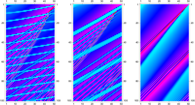
Figure 1: Time evolutions of the closed geometric crystal chain for $n=2$ and $L=50$. The values of the parameters are $s=1$ (All), and $l=0.00001$ (Left), $l=0.1$ (Middle), $l=2.0$ (Right). The initial state is given by $b_{i}=i/10\quad(1\leq i\leq 50)$ at the top row, and the time flows from top to bottom. Visualization is produced by the command MatrixPlot in Mathematica${}^{\scriptstyle\mbox{\scriptsize\textregistered}}$.

By repeated use of the Yang-Baxter relation $R_{i+1}^{(s,l_{2})}R_{i}^{(s,l_{1})}R_{i+1}^{(l_{2},l_{1})}=R_{i}^{(l_{2},l_{1})}R_{i+1}^{(s,l_{1})}R_{i}^{(s,l_{2})}$ and the involution $R_{L+1}^{(l_{2},l_{1})}\circ R_{L+1}^{(l_{1},l_{2})}={\rm Id}$, we obtain

$$(R_{2}^{(s,l_{2})}\circ\dots\circ R_{L+1}^{(s,l_{2})})\circ(R_{1}^{(s,l_{1})}\circ\dots\circ R_{L}^{(s,l_{1})})$$

$$\quad=R_{2}^{(s,l_{2})}\circ R_{1}^{(s,l_{1})}\circ R_{3}^{(s,l_{2})}\circ R_{2}^{(s,l_{1})}\circ\dots\circ R_{L+1}^{(s,l_{2})}\circ R_{L}^{(s,l_{1})}$$

$$\quad=(R_{2}^{(s,l_{2})}\circ R_{1}^{(s,l_{1})}\circ R_{3}^{(s,l_{2})}\circ R_{2}^{(s,l_{1})}\circ\dots\circ R_{L+1}^{(s,l_{2})}\circ R_{L}^{(s,l_{1})})\circ(R_{L+1}^{(l_{2},l_{1})}\circ R_{L+1}^{(l_{1},l_{2})})$$

$$\quad=R_{1}^{(l_{2},l_{1})}\circ(R_{2}^{(s,l_{1})}\circ R_{1}^{(s,l_{2})}\circ R_{3}^{(s,l_{1})}\circ R_{2}^{(s,l_{2})}\circ\dots\circ R_{L+1}^{(s,l_{1})}\circ R_{L}^{(s,l_{2})})\circ R_{L+1}^{(l_{1},l_{2})}$$

$$\quad=R_{1}^{(l_{2},l_{1})}\circ(R_{2}^{(s,l_{1})}\circ\dots\circ R_{L+1}^{(s,l_{1})})\circ(R_{1}^{(s,l_{2})}\circ\dots\circ R_{L}^{(s,l_{2})})\circ R_{L+1}^{(l_{1},l_{2})}.$$

By substituting this into (12) we obtain

$$(R_{2}^{(s,l_{1})}\circ\dots\circ R_{L+1}^{(s,l_{1})})\circ(R_{1}^{(s,l_{2})}\circ\dots\circ R_{L}^{(s,l_{2})})(b_{1},\dots,b_{L},u,\tilde{u})=(u,\tilde{u},b^{\prime\prime}_{1},\dots,b^{\prime\prime}_{L}),$$ (13)

where $(u,\tilde{u})=R^{(l_{1},l_{2})}(v,\tilde{v})$. Therefore we have $T_{l_{1}}\circ T_{l_{2}}(b_{1},\dots,b_{L})=(b^{\prime\prime}_{1},\dots,b^{\prime\prime}_{L})$.

2.2.2 Conservation laws.

Here we show that the closed geometric crystal chains are discrete integrable systems with $L/2$ (resp. $(L+1)/2$) conserved quantities for even (resp. odd) $L$.

Given $a,b\in{\mathbb{R}}_{>0}$, the $a^{\prime},b^{\prime}$ in (4) are determined by a pair of equations

$$ab=a^{\prime}b^{\prime},\qquad b+\frac{l}{a}=a^{\prime}+\frac{s}{b^{\prime}}.$$ (14)

It is equivalent to the following matrix equation

$$\begin{pmatrix}b&\lambda\\ 1&s/b\end{pmatrix}\begin{pmatrix}a&\lambda\\ 1&l/a\end{pmatrix}=\begin{pmatrix}a^{\prime}&\lambda\\ 1&l/a^{\prime}\end{pmatrix}\begin{pmatrix}b^{\prime}&\lambda\\ 1&s/b^{\prime}\end{pmatrix},$$ (15)

where $\lambda$ is a parameter called the loop parameter [2]. Thus for the choice of $v$ in (9), the equation depicted by (5) is written as

$$\begin{pmatrix}b_{1}&\lambda\\ 1&s/b_{1}\end{pmatrix}\cdots\begin{pmatrix}b_{L}&\lambda\\ 1&s/b_{L}\end{pmatrix}\begin{pmatrix}v&\lambda\\ 1&l/v\end{pmatrix}=\begin{pmatrix}v&\lambda\\ 1&l/v\end{pmatrix}\begin{pmatrix}b^{\prime}_{1}&\lambda\\ 1&s/b^{\prime}_{1}\end{pmatrix}\cdots\begin{pmatrix}b^{\prime}_{L}&\lambda\\ 1&s/b^{\prime}_{L}\end{pmatrix}.$$ (16)

Define $g(\alpha,\beta;\lambda)$ and $\mathcal{L}(|b\rangle;\lambda)$ for $|b\rangle:=(b_{1},\dots,b_{L})$ to be $2\times 2$ matrices given by

$$g(\alpha,\beta;\lambda):=\begin{pmatrix}\alpha&\lambda\\ 1&\beta/\alpha\end{pmatrix},\quad\mathcal{L}(|b\rangle;\lambda)=\begin{pmatrix}L_{11}(\lambda)&L_{12}(\lambda)\\ L_{21}(\lambda)&L_{22}(\lambda)\end{pmatrix}:=g(b_{1},s;\lambda)\cdots g(b_{L},s;\lambda).$$ (17)

Then equation (16) is written as

$$\mathcal{L}(T_{l}|b\rangle;\lambda)=g(v,l;\lambda)^{-1}\mathcal{L}(|b\rangle;\lambda)g(v,l;\lambda),$$ (18)

which can be viewed as a discrete time analogue of the Lax equation [25]. This implies that the characteristic polynomial

$$\det(x\mathbb{I}_{2}-\mathcal{L}(|b\rangle;\lambda))=x^{2}-(L_{11}(\lambda)+L_{22}(\lambda))x+\det\mathcal{L}(|b\rangle;\lambda)$$

is invariant under the time evolution $T_{l}$ for any $l\in{\mathbb{R}}_{>0}$. Since $\det\mathcal{L}(|b\rangle;\lambda)=(s-\lambda)^{L}$ is trivially conserved, all the non-trivial conserved quantities of this dynamical system are contained in the trace $L_{11}(\lambda)+L_{22}(\lambda)$.

Let $b_{j}^{(1)}=b_{j},b_{j}^{(2)}=s/b_{j}$ and for any $m\in{\mathbb{Z}}$ we extend its definition by $b_{j}^{(m)}=b_{j}^{(m-2)}$. Based on [9, 19], define the loop elementary symmetric functions $e^{(r)}_{m}(|b\rangle)\,(r=0,1)$ by

$$e^{(1)}_{m}(|b\rangle) =\sum_{1\leq j_{1}<j_{2}<\dots<j_{m}\leq L}b_{j_{1}}^{(2-j_{1})}b_{j_{2}}^{(3-j_{2})}\cdots b_{j_{m}}^{(1+m-j_{m})},$$

$$e^{(0)}_{m}(|b\rangle) =\sum_{1\leq j_{1}<j_{2}<\dots<j_{m}\leq L}b_{j_{1}}^{(1-j_{1})}b_{j_{2}}^{(2-j_{2})}\cdots b_{j_{m}}^{(m-j_{m})},$$ (19)

and $e^{(r)}_{0}(|b\rangle)=1,\,e^{(r)}_{m}(|b\rangle)=0\,(m<0)$. By Lemma 6.1 of [9], we have

$$L_{11}(\lambda)=\sum_{m\geq 0}e^{(1)}_{L-2m}(|b\rangle)\lambda^{m},\quad L_{12}(\lambda)=\sum_{m>0}e^{(1)}_{L+1-2m}(|b\rangle)\lambda^{m},$$

$$L_{21}(\lambda)=\sum_{m\geq 0}e^{(0)}_{L-1-2m}(|b\rangle)\lambda^{m},\quad L_{22}(\lambda)=\sum_{m\geq 0}e^{(0)}_{L-2m}(|b\rangle)\lambda^{m}.$$ (20)

Since the parameter $\lambda$ can take arbitrary values, every coefficient

$$I_{L-2m}:=e^{(1)}_{L-2m}(|b\rangle)+e^{(0)}_{L-2m}(|b\rangle),$$ (21)

in the polynomial $L_{11}(\lambda)+L_{22}(\lambda)$ is a conserved quantity. To summarize, there are $(L+1)/2$ conserved quantities $I_{1},I_{3},\dots,I_{L}$ for odd $L$, and $L/2$ conserved quantities $I_{2},I_{4},\dots,I_{L}$ for even $L$, besides the trivial one $I_{0}=2$.

Example 3

The traces $L_{11}(\lambda)+L_{22}(\lambda)$ for up to $L=4$ are as follows:

$$L=1: \quad b_{1}+\bar{b}_{1},$$ (22)

$$L=2: \quad 2\lambda+b_{1}b_{2}+\bar{b}_{1}\bar{b}_{2},$$ (23)

$$L=3: \quad\lambda(b_{1}+\bar{b}_{1}+b_{2}+\bar{b}_{2}+b_{3}+\bar{b}_{3})+b_{1}b_{2}b_{3}+\bar{b}_{1}\bar{b}_{2}\bar{b}_{3},$$ (24)

$$L=4: \quad 2\lambda^{2}+\lambda(b_{1}b_{2}+b_{1}\bar{b}_{3}+b_{1}b_{4}+\bar{b}_{2}\bar{b}_{3}+\bar{b}_{2}b_{4}+b_{3}b_{4}$$

$$\quad+\bar{b}_{1}\bar{b}_{2}+\bar{b}_{1}b_{3}+\bar{b}_{1}\bar{b}_{4}+b_{2}b_{3}+b_{2}\bar{b}_{4}+\bar{b}_{3}\bar{b}_{4})+b_{1}b_{2}b_{3}b_{4}+\bar{b}_{1}\bar{b}_{2}\bar{b}_{3}\bar{b}_{4}.$$ (25)

Here $\bar{b}_{i}$ denotes $s/b_{i}$.

By taking $\lambda=0$ in (16), we see that $I^{\prime}_{L}:=e^{(1)}_{L}(|b\rangle)=b_{1}\dots b_{L}$ is also a conserved quantity, which can be used in place of $I_{L}$.

Remark 4

In the case of even $L$, the quantity $I^{\prime}_{1}:=e^{(1)}_{1}(|b\rangle)=b_{1}+\bar{b}_{2}+\dots+b_{L-1}+\bar{b}_{L}$ is invariant under any two consecutive time evolutions $T_{l_{2}}\circ T_{l_{1}}(b_{1},\dots,b_{L})=(b^{\prime\prime}_{1},\dots,b^{\prime\prime}_{L})$. This claim is verified by considering the equation $\mathcal{L}(|b\rangle;\lambda)g(v,l_{1};\lambda)g(\tilde{v},l_{2};\lambda)=g(v,l_{1};\lambda)g(\tilde{v},l_{2};\lambda)\mathcal{L}(|b^{\prime\prime}\rangle;\lambda)$, divided by $\lambda^{L/2+1}$ and then by taking the limit $\lambda\rightarrow\infty$. Since $e^{(1)}_{1}(|b\rangle)e^{(0)}_{1}(|b\rangle)=Ls+I_{2}$ is a conserved quantity, the quantity $\bar{I}^{\prime}_{1}:=e^{(0)}_{1}(|b\rangle)=\bar{b}_{1}+b_{2}+\dots+\bar{b}_{L-1}+b_{L}$ has also this property.

2.2.3 Invertibility.

The time evolution $T_{l}$ defined in (11) is invertible. Actually, given any $(b_{1},\dots,b_{L})\in({\mathbb{R}}_{>0})^{L}$ one can obtain $(T_{l})^{-1}(b_{1},\cdots,b_{L})=(\tilde{b}_{1},\cdots,\tilde{b}_{L})$ in the following way. In view of (16) we begin with the matrix equation

$$\begin{pmatrix}\tilde{b}_{1}&\lambda\\ 1&s/\tilde{b}_{1}\end{pmatrix}\cdots\begin{pmatrix}\tilde{b}_{L}&\lambda\\ 1&s/\tilde{b}_{L}\end{pmatrix}\begin{pmatrix}\tilde{v}&\lambda\\ 1&l/\tilde{v}\end{pmatrix}=\begin{pmatrix}\tilde{v}&\lambda\\ 1&l/\tilde{v}\end{pmatrix}\begin{pmatrix}L_{11}(\lambda)&L_{12}(\lambda)\\ L_{21}(\lambda)&L_{22}(\lambda)\end{pmatrix},$$ (26)

where $\tilde{v}$ and $\tilde{b}_{i}$’s are the unknowns. By flipping the matrices with respect to their anti-diagonals, we see that this equation is equivalent to

$$\begin{pmatrix}l/\tilde{v}&\lambda\\ 1&\tilde{v}\end{pmatrix}\begin{pmatrix}s/\tilde{b}_{L}&\lambda\\ 1&\tilde{b}_{L}\end{pmatrix}\cdots\begin{pmatrix}s/\tilde{b}_{1}&\lambda\\ 1&\tilde{b}_{1}\end{pmatrix}=\begin{pmatrix}L_{22}(\lambda)&L_{12}(\lambda)\\ L_{21}(\lambda)&L_{11}(\lambda)\end{pmatrix}\begin{pmatrix}l/\tilde{v}&\lambda\\ 1&\tilde{v}\end{pmatrix}.$$ (27)

In the same way as in Proposition 2 to obtain (9), we see that the $\tilde{v}$ satisfying this matrix equation is determined by the following equation

$$l/\tilde{v}=\frac{L_{22}l/\tilde{v}+L_{12}}{L_{21}l/\tilde{v}+L_{11}},$$

where $L_{ij}=L_{ij}(l)$s are given by (7). Its unique positive real solution is

$$\tilde{v}=\frac{2lL_{21}}{L_{22}-L_{11}+\sqrt{(L_{11}-L_{22})^{2}+4L_{12}L_{21}}}.$$ (28)

With this choice of $\tilde{v}$ we can obtain the $(\tilde{b}_{1},\dots,\tilde{b}_{L})$ in (26) by using the inverse map $\mathcal{R}^{-1}=R_{L}\circ\cdots\circ R_{1}$ as $\mathcal{R}^{-1}(\tilde{v},b_{1},\dots,b_{L})=(\tilde{b}_{1},\dots,\tilde{b}_{L},\tilde{v})$.

2.3 Continuum limits and associated differential equations

2.3.1 A naive method.

In order to observe a few of the properties of our new discrete dynamical system, we consider two different continuum limits of the system. First we note that this system has an obvious scale invariance. That is, by replacing $a,b,s,l$ in (4) by $\mu a,\mu b,\mu^{2}s,\mu^{2}l$ with a parameter $\mu\in{\mathbb{R}}_{>0}$ results in the replacements of $a^{\prime},b^{\prime}$ by $\mu a^{\prime},\mu b^{\prime}$. So, we may set $s=1$, and we also use the letter $\tau$ instead of $l$. Under this setting, we rewrite the equations in (14) as

$$ab=a^{\prime}b^{\prime},\qquad b+\frac{\tau}{a}=a^{\prime}+\frac{1}{b^{\prime}}.$$ (29)

The first method is a naive one in which we respect neither the integrability nor the periodicity of the system. Let $u(x,t),v(x,t)$ be a pair of variables depending on time $t$ and position $x$, and $\delta>0$ a small variable. We set

$$a =v(x+c_{0}\delta,t),\quad b=u(x,t-\delta),$$

$$a^{\prime} =v(x-c_{0}\delta,t),\quad b^{\prime}=u(x,t+\delta),$$

and require that both equations in (29) are satisfied up to order $1$ of the variable $\delta$. This requirement is satisfied if the variables $u(x,t),v(x,t)$ satisfy the following differential equation

$$\frac{\partial_{t}u(x,t)}{u(x,t)}=c_{0}\frac{\partial_{x}v(x,t)}{v(x,t)},$$ (30)

and if they are expressed by a new variable $U(x,t)$ as

$$v(x,t)=\sinh\left[U(x,t)\right]+\sqrt{\tau+\sinh^{2}\left[U(x,t)\right]},$$ (31)

$$u(x,t)=\exp\left[U(x,t)\right].$$ (32)

Putting them together we obtain the following partial differential equation

$$\frac{1}{c_{0}}\frac{\partial U(x,t)}{\partial t}=\frac{\cosh\left[U(x,t)\right]}{\sqrt{\tau+\sinh^{2}\left[U(x,t)\right]}}\frac{\partial U(x,t)}{\partial x}.$$ (33)

This is a sort of nonlinear advection equation. When $\tau=1$ it reduces the linear differential equation $\partial_{t}U=c_{0}\partial_{x}U$ for left moving waves of a common velocity $c_{0}$, in agreement with the cyclic shift behavior of the original discrete dynamical system for the case of time evolution $T_{s}$.

2.3.2 Another method to respect the integrability.

Here we assume that $L$ is an odd integer. According to diagram (5) we write the evolution equation as

$$v_{i+1}b_{i}=v_{i}b^{\prime}_{i},\qquad b_{i}+\frac{\tau}{v_{i+1}}=v_{i}+\frac{1}{b^{\prime}_{i}}.$$ (34)

Let $a_{i}(t),u_{i}(t)$ be a pair of variables depending on time $t$ and position $i\in{\mathbb{Z}}/L{\mathbb{Z}}$, $C$ a constant, and $\delta>0$ a small variable. We set

$$v_{i+1} =\frac{1}{\delta}+a_{i+1}(t),\quad b_{i}=u_{i}(t),$$

$$v_{i} =\frac{1}{\delta}+a_{i}(t),\qquad b^{\prime}_{i}=u_{i}(t+\delta),$$

$$\tau =\frac{1}{\delta^{2}}+\frac{C}{\delta},$$

and write (34) as the following discrete time analogue of the Lax triads [25]

$$g(b_{i}^{\prime},1;\lambda)=(\delta\cdot g(v_{i},\tau;\lambda))^{-1}g(b_{i},1;\lambda)(\delta\cdot g(v_{i+1},\tau;\lambda)),$$ (35)

where $g(\bullet,\bullet;\lambda)$ is the $2\times 2$ matrix defined in (17). Since $\delta\cdot g(v_{i},\tau;\lambda)=\mathbb{I}_{2}+\delta\cdot h(a_{i}(t),C;\lambda)+\mathcal{O}(\delta^{2})$ where

$$h(\alpha,\beta;\lambda)=\begin{pmatrix}\alpha&\lambda\\ 1&\beta-\alpha\end{pmatrix},$$ (36)

one can derive the following (continuous time) Lax triads [25]

$$\frac{{\rm d}}{{\rm d}t}g(u_{i}(t),1;\lambda)=g(u_{i}(t),1;\lambda)h(a_{i+1}(t),C;\lambda)-h(a_{i}(t),C;\lambda)g(u_{i}(t),1;\lambda).$$ (37)

This implies that

$$a_{i+1}(t)+a_{i}(t) =u_{i}(t)-\frac{1}{u_{i}(t)}+C,$$

$$\frac{{\rm d}}{{\rm d}t}u_{i}(t) =u_{i}(t)(a_{i+1}(t)-a_{i}(t)).$$

Since $L$ is odd, we can solve the first couple of equations as

$$a_{i}(t)=\frac{1}{2}\sum_{j=0}^{L-1}(-1)^{j}\left(u_{i+j}(t)-\frac{1}{u_{i+j}(t)}\right)+\frac{C}{2}.$$

By substituting this expression in the second equation, we have

$$\frac{{\rm d}}{{\rm d}t}u_{i}(t)=u_{i}(t)\sum_{j=1}^{L-1}(-1)^{j-1}\left(u_{i+j}(t)-\frac{1}{u_{i+j}(t)}\right).$$

This may be viewed as a variation of the Lotka-Volterra equation. If we set $u_{i}(t)=\exp[U_{i}(t)]$, the equation is written as

$$\frac{{\rm d}}{{\rm d}t}U_{i}(t)=2\sum_{j=1}^{L-1}(-1)^{j-1}\sinh U_{i+j}(t).$$ (38)

This system has obvious conserved quantities $\sum_{j=1}^{L}U_{i}(t)$ and $\sum_{j=1}^{L}\cosh U_{i}(t)$.

A continuous limit of the discrete Lax equation (18) is obtained by a standard method. Let $\mathcal{L}(t)=g(u_{1}(t),1;\lambda)\cdots g(u_{L}(t),1;\lambda)$ and $\mathcal{B}(t)=h(a_{1}(t),C;\lambda)$. Then we obtain

$$\frac{{\rm d}}{{\rm d}t}\mathcal{L}(t)=[\mathcal{L}(t),\mathcal{B}(t)],$$ (39)

from the Lax triads equation (37).

2.4 Tropicalization and piecewise linear formulas

2.4.1 An equation for periodic boundary conditions.

Tropicalization is a procedure for turning subtraction-free rational maps $({\mathbb{R}}_{>0})^{d_{1}}\rightarrow({\mathbb{R}}_{>0})^{d_{2}}$ into piecewise-linear maps ${\mathbb{R}}^{d_{1}}\rightarrow{\mathbb{R}}^{d_{2}}$ by replacing the operations $+,\cdot,\div$ with the operations min, $+,-$, and ignoring constants. In fact, there are some variations of the notion of tropicalization. We adopt one of them which was described in [8]. With an infinitesimal parameter $\varepsilon>0$, define $\mathrm{Log}_{\varepsilon}:{\mathbb{R}}_{>0}\to{\mathbb{R}}$ to be a map given by

$$\mathrm{Log}_{\varepsilon}:a\mapsto-\varepsilon\log a.$$ (40)

For $a,b>0$ define $\mathsf{Trop}({a}),\mathsf{Trop}({b})\in{\mathbb{R}}$ by $a=\rme^{-\frac{\mathsf{Trop}({a})}{\varepsilon}}$ and $b=\rme^{-\frac{\mathsf{Trop}({b})}{\varepsilon}}$. Then we have

$$\mathrm{Log}_{\varepsilon}(a+b)=-\varepsilon\log(\rme^{-\frac{\mathsf{Trop}({a})}{\varepsilon}}+\rme^{-\frac{\mathsf{Trop}({b})}{\varepsilon}}),\quad\mathrm{Log}_{\varepsilon}(a\times b)=\mathsf{Trop}({a})+\mathsf{Trop}({b}).$$

In the limit $\varepsilon\to 0$, $\mathrm{Log}_{\varepsilon}(a+b)$ becomes $\min(\mathsf{Trop}({a}),\mathsf{Trop}({b}))$. In this manner, the algebra $({\mathbb{R}}_{>0},+,\times)$ reduces to the so called min-plus algebra, and the procedure $\lim_{\varepsilon\to 0}\mathrm{Log}_{\varepsilon}$ with the transformation as $a=\rme^{-\frac{\mathsf{Trop}({a})}{\varepsilon}}$ turns out to be the above mentioned tropicalization.

For example, the map of geometric $R$-matrix (4) is tropicalized to the following piecewise linear map

$$A^{\prime} =A+\min(B,\mathsf{Trop}({l})-A)-\min(A,\mathsf{Trop}({s})-B),$$

$$B^{\prime} =B+\min(A,\mathsf{Trop}({s})-B)-\min(B,\mathsf{Trop}({l})-A),$$ (41)

where $A=\mathsf{Trop}({a}),B=\mathsf{Trop}({b})$ and so on. When we let the values of the variables be restricted to ${\mathbb{Z}}_{\geq 0}$, this reduces to the simplest case of the combinatorial $R$-matrix in Kashiwara’s crystal. It is described by one-row tableaux of two kinds of letters (1 and 2)

$$\overbrace{1\dots 1}^{B}\overbrace{2\dots 2}^{\mathsf{Trop}({s})-B}\otimes\overbrace{1\dots 1}^{A}\overbrace{2\dots 2}^{\mathsf{Trop}({l})-A}\mapsto\overbrace{1\dots 1}^{A^{\prime}}\overbrace{2\dots 2}^{\mathsf{Trop}({l})-A^{\prime}}\otimes\overbrace{1\dots 1}^{B^{\prime}}\overbrace{2\dots 2}^{\mathsf{Trop}({s})-B^{\prime}}.$$ (42)

The generalized periodic box-ball system [14, 26] may be regarded as a tropicalization of the closed geometric crystal chain in section 2.1. Compared with the diagram (5), the corresponding situation may be depicted by

      (43)

where $V=\mathsf{Trop}({v})$, $B_{i}=\mathsf{Trop}({b_{i}})$ and so on. However, the assertion of Lemma 2 which tells the existence of a unique solution to the equation $V_{1}=V$, does not persist in the tropicalization. This is due to the fact that the expression for $v$ in (9) is not subtraction-free rational. Therefore, to study the periodic boundary condition for the generalized periodic box-ball system, we have to consider the tropicalization of the equation (8) itself. It reads as

$$V=\min(\Lambda_{11}+V,\Lambda_{12})-\min(\Lambda_{21}+V,\Lambda_{22}).$$ (44)

Here

$$\Lambda_{ij}=\mathsf{Trop}({L_{ij}})=\mathsf{Trop}({L_{ij}(l)}),$$ (45)

that are tropicalizations of the matrix elements of the monodromy matrix (7). They can be explicitly written down by using the loop elementary symmetric functions (19) and (20).

Example 5

The $\Lambda_{11},\Lambda_{21}$ for up to $L=4$ are as follows:

$$L=1: \quad\Lambda_{11}=B_{1},\Lambda_{21}=0,$$

$$L=2: \quad\Lambda_{11}=\min(\mathsf{Trop}({l}),B_{1}+B_{2}),\Lambda_{21}=\min(\bar{B}_{1},B_{2}),$$

$$L=3: \quad\Lambda_{11}=\min(\mathsf{Trop}({l})+\min(B_{1},\bar{B}_{2},B_{3}),B_{1}+B_{2}+B_{3}),$$

$$\quad\Lambda_{21}=\min(\mathsf{Trop}({l}),\bar{B}_{1}+\bar{B}_{2},\bar{B}_{1}+B_{3},B_{2}+B_{3}),$$

$$L=4: \quad\Lambda_{11}=\min\left(2\mathsf{Trop}({l}),\mathsf{Trop}({l})+\min(B_{1}+B_{2},B_{1}+\bar{B}_{3},B_{1}+B_{4},\right.$$

$$\quad\quad\quad\quad\quad\quad\left.\bar{B}_{2}+\bar{B}_{3},\bar{B}_{2}+B_{4},B_{3}+B_{4}\right),B_{1}+B_{2}+B_{3}+B_{4}),$$

$$\quad\Lambda_{21}=\min(\mathsf{Trop}({l})+\min(\bar{B}_{1},B_{2},\bar{B}_{3},B_{4}),$$

$$\quad\quad\quad\quad\quad\quad\bar{B}_{1}+\bar{B}_{2}+\bar{B}_{3},\bar{B}_{1}+\bar{B}_{2}+B_{4},\bar{B}_{1}+B_{3}+B_{4},B_{2}+B_{3}+B_{4}).$$

Here $\bar{B}_{i}$ denotes $\mathsf{Trop}({s})-B_{i}$. The other matrix elements are given by $\Lambda_{22}=\Lambda_{11}(B_{i}\leftrightarrow\bar{B}_{i}),\Lambda_{12}=\mathsf{Trop}({l})+\Lambda_{21}(B_{i}\leftrightarrow\bar{B}_{i})$.

The following result is easily obtained by a simple case-by-case check.

Proposition 6

The solution to the equation (44) is given by:

1. If $\frac{\Lambda_{12}+\Lambda_{21}}{2}\leq\min(\Lambda_{11},\Lambda_{22})$, then $V=\frac{\Lambda_{12}-\Lambda_{21}}{2}$.

2. If $\Lambda_{11}<\min(\Lambda_{22},\frac{\Lambda_{12}+\Lambda_{21}}{2})$, then $V=\Lambda_{11}-\Lambda_{21}$.

3. If $\Lambda_{22}<\min(\Lambda_{11},\frac{\Lambda_{12}+\Lambda_{21}}{2})$, then $V=\Lambda_{12}-\Lambda_{22}$.

4. If $\Lambda_{11}=\Lambda_{22}<\frac{\Lambda_{12}+\Lambda_{21}}{2}$, then any $V$ such that $\Lambda_{11}-\Lambda_{21}\leq V\leq\Lambda_{12}-\Lambda_{11}$.

Proof. For simplicity, let $A=\Lambda_{11},B=\Lambda_{12},C=\Lambda_{21}$ and $D=\Lambda_{22}$.

Case (i): Suppose $C+V>D$. Then we have $V>D-C\geq\frac{B+C}{2}-C=\frac{B-C}{2}$, hence $A+V>\frac{B+C}{2}+\frac{B-C}{2}=B$. So by (44) we get $V=B-D$, but this leads to $D<C+V=C+B-D\leq 2D-D=D$, a contradiction. Thus $C+V\leq D$. Suppose $A+V<B$, which implies $V=A-C$ by (44). But this leads to $B>A+V=2A-C\geq B+C-C=B$, a contradiction. Therefore $A+V\geq B$, hence by (44) we get $V=\frac{B-C}{2}$.

Case (ii): Suppose $A+V>B$. Then if $C+V\geq D$ we get $V=B-D$ by (44), which leads to $B<A+V=A+B-D<B$, a contradiction. Otherwise we have $C+V<D$ and then $V=\frac{B-C}{2}$ by (44), which leads to $B<A+V<\frac{B+C}{2}+\frac{B-C}{2}=B$, a contradiction. Thus $A+V\leq B$. Then if $C+V>D$ we have $A=D$ by (44) that contradicts to the assumption. Therefore $C+V\leq D$, hence by (44) we get $V=A-C$.

Case (iii): A proof can be obtained from the previous case by exchanging $A$ with $D$, $B$ with $C$, and $V$ with $-V$.

Case (iv): Suppose $A+V>B$. Then if $C+V>D$ we get $V=B-D$ by (44), which leads to $B<A+V=A+B-D=B$, a contradiction. Otherwise we have $C+V\leq D$ and then $V=\frac{B-C}{2}$ by (44), which leads to $D\geq C+V=\frac{B+C}{2}>D$, a contradiction. Thus $A+V\leq B$. Then if $C+V<D$ we have $V=A-C$ by (44), which leads to $D>C+V=A=D$, a contradiction. Therefore $C+V\geq D$, hence by (44) we get $A=D$ which does not contradict to the assumption. Thus any $V$ satisfying the condition $A-C\leq V\leq B-A$ solves the equation (44). $\Box$

Here we show two examples to examine this result.

Example 7

Set $L=2,\mathsf{Trop}({s})=2$, and $B_{1}=B_{2}=1$. This is the state $12\otimes 12$ in tableau notation. By Example 5 one has $\Lambda_{11}=\Lambda_{22}=\min(\mathsf{Trop}({l}),2)$, and $\frac{\Lambda_{12}+\Lambda_{21}}{2}=1+\mathsf{Trop}({l})/2$. Hence it falls into either case (i) when $\mathsf{Trop}({l})=2$ or into case (iv) otherwise. In any case the solution is given by $\min(\mathsf{Trop}({l})-1,1)\leq V\leq\max(\mathsf{Trop}({l})-1,1)$. In particular, when $\mathsf{Trop}({l})=1$ we have $V=0$ and $V=1$ as possible solutions of integer values. Then the diagram (43) reads as

$$\begin{picture}(40.0,40.0)(-20.0,-20.0)\put(-10.0,0.0){\line(1,0){20.0}} \put(0.0,10.0){\line(0,-1){20.0}} \put(-11.0,0.0){\makebox(0.0,0.0)[r]{$1$}} \put(0.0,11.0){\makebox(0.0,0.0)[b]{$1$}} \put(0.0,-11.0){\makebox(0.0,0.0)[t]{$0$}} \put(11.0,0.0){\makebox(0.0,0.0)[l]{$0$}} \end{picture}\!\!\!\!\!\!\begin{picture}(40.0,40.0)(-20.0,-20.0)\put(-10.0,0.0){\line(1,0){20.0}} \put(0.0,10.0){\line(0,-1){20.0}} \put(-11.0,0.0){\makebox(0.0,0.0)[r]{$$}} \put(0.0,11.0){\makebox(0.0,0.0)[b]{$1$}} \put(0.0,-11.0){\makebox(0.0,0.0)[t]{$2$}} \put(11.0,0.0){\makebox(0.0,0.0)[l]{$1$}} \end{picture}\qquad\begin{picture}(40.0,40.0)(-20.0,-20.0)\put(0.0,-1.0){\makebox(0.0,0.0)[b]{and}} \end{picture}\qquad\begin{picture}(40.0,40.0)(-20.0,-20.0)\put(-10.0,0.0){\line(1,0){20.0}} \put(0.0,10.0){\line(0,-1){20.0}} \put(-11.0,0.0){\makebox(0.0,0.0)[r]{$0$}} \put(0.0,11.0){\makebox(0.0,0.0)[b]{$1$}} \put(0.0,-11.0){\makebox(0.0,0.0)[t]{$2$}} \put(11.0,0.0){\makebox(0.0,0.0)[l]{$1$}} \end{picture}\!\!\!\!\!\!\begin{picture}(40.0,40.0)(-20.0,-20.0)\put(-10.0,0.0){\line(1,0){20.0}} \put(0.0,10.0){\line(0,-1){20.0}} \put(-11.0,0.0){\makebox(0.0,0.0)[r]{$$}} \put(0.0,11.0){\makebox(0.0,0.0)[b]{$1$}} \put(0.0,-11.0){\makebox(0.0,0.0)[t]{$0$}} \put(11.0,0.0){\makebox(0.0,0.0)[l]{$0$}} \end{picture},$$

respectively. The periodic boundary condition $V_{1}=V$ is indeed satisfied, but the output states ($22\otimes 11$ and $11\otimes 22$ in tableau notation) are different. So, we can not define a unique time evolution compatible with such periodic boundary conditions.

Example 8

Set $L=3,\mathsf{Trop}({s})=2$, and $B_{1}=B_{2}=B_{3}=1$. This is the state $12\otimes 12\otimes 12$ in tableau notation. By Example 5 one has $\Lambda_{11}=\Lambda_{22}=1+\min(\mathsf{Trop}({l}),2)$, and $\frac{\Lambda_{12}+\Lambda_{21}}{2}=\min(\mathsf{Trop}({l}),2)+\mathsf{Trop}({l})/2$. Hence it falls into either case (i) when $\mathsf{Trop}({l})=1,2$ or into case (iv) otherwise. In the former case the solution is given by $V=\mathsf{Trop}({l})/2$, and in the latter case it is given by $1\leq V\leq\mathsf{Trop}({l})-1$. In particular, when $\mathsf{Trop}({l})=1$ we have $V=1/2$ as the solution, but it is not an integer:

$$\begin{picture}(40.0,40.0)(-20.0,-20.0)\put(-10.0,0.0){\line(1,0){20.0}} \put(0.0,10.0){\line(0,-1){20.0}} \put(-11.0,0.0){\makebox(0.0,0.0)[r]{$\frac{1}{2}$}} \put(0.0,11.0){\makebox(0.0,0.0)[b]{$1$}} \put(0.0,-11.0){\makebox(0.0,0.0)[t]{$1$}} \put(11.0,0.0){\makebox(0.0,0.0)[l]{$\frac{1}{2}$}} \end{picture}\!\!\!\!\!\!\begin{picture}(40.0,40.0)(-20.0,-20.0)\put(-10.0,0.0){\line(1,0){20.0}} \put(0.0,10.0){\line(0,-1){20.0}} \put(-11.0,0.0){\makebox(0.0,0.0)[r]{$$}} \put(0.0,11.0){\makebox(0.0,0.0)[b]{$1$}} \put(0.0,-11.0){\makebox(0.0,0.0)[t]{$1$}} \put(11.0,0.0){\makebox(0.0,0.0)[l]{$\frac{1}{2}$}} \end{picture}\!\!\!\!\!\!\begin{picture}(40.0,40.0)(-20.0,-20.0)\put(-10.0,0.0){\line(1,0){20.0}} \put(0.0,10.0){\line(0,-1){20.0}} \put(-11.0,0.0){\makebox(0.0,0.0)[r]{$$}} \put(0.0,11.0){\makebox(0.0,0.0)[b]{$1$}} \put(0.0,-11.0){\makebox(0.0,0.0)[t]{$1$}} \put(11.0,0.0){\makebox(0.0,0.0)[l]{$\frac{1}{2}$}} \end{picture}.$$

In fact, the only possible diagram (43) for integer value $V$ is given by

$$\begin{picture}(40.0,40.0)(-20.0,-20.0)\put(-10.0,0.0){\line(1,0){20.0}} \put(0.0,10.0){\line(0,-1){20.0}} \put(-11.0,0.0){\makebox(0.0,0.0)[r]{$1$}} \put(0.0,11.0){\makebox(0.0,0.0)[b]{$1$}} \put(0.0,-11.0){\makebox(0.0,0.0)[t]{$0$}} \put(11.0,0.0){\makebox(0.0,0.0)[l]{$0$}} \end{picture}\!\!\!\!\!\!\begin{picture}(40.0,40.0)(-20.0,-20.0)\put(-10.0,0.0){\line(1,0){20.0}} \put(0.0,10.0){\line(0,-1){20.0}} \put(-11.0,0.0){\makebox(0.0,0.0)[r]{$$}} \put(0.0,11.0){\makebox(0.0,0.0)[b]{$1$}} \put(0.0,-11.0){\makebox(0.0,0.0)[t]{$2$}} \put(11.0,0.0){\makebox(0.0,0.0)[l]{$1$}} \end{picture}\!\!\!\!\!\!\begin{picture}(40.0,40.0)(-20.0,-20.0)\put(-10.0,0.0){\line(1,0){20.0}} \put(0.0,10.0){\line(0,-1){20.0}} \put(-11.0,0.0){\makebox(0.0,0.0)[r]{$$}} \put(0.0,11.0){\makebox(0.0,0.0)[b]{$1$}} \put(0.0,-11.0){\makebox(0.0,0.0)[t]{$0$}} \put(11.0,0.0){\makebox(0.0,0.0)[l]{$0$}} \end{picture}\qquad\begin{picture}(40.0,40.0)(-20.0,-20.0)\put(0.0,-1.0){\makebox(0.0,0.0)[b]{or}} \end{picture}\qquad\begin{picture}(40.0,40.0)(-20.0,-20.0)\put(-10.0,0.0){\line(1,0){20.0}} \put(0.0,10.0){\line(0,-1){20.0}} \put(-11.0,0.0){\makebox(0.0,0.0)[r]{$0$}} \put(0.0,11.0){\makebox(0.0,0.0)[b]{$1$}} \put(0.0,-11.0){\makebox(0.0,0.0)[t]{$2$}} \put(11.0,0.0){\makebox(0.0,0.0)[l]{$1$}} \end{picture}\!\!\!\!\!\!\begin{picture}(40.0,40.0)(-20.0,-20.0)\put(-10.0,0.0){\line(1,0){20.0}} \put(0.0,10.0){\line(0,-1){20.0}} \put(-11.0,0.0){\makebox(0.0,0.0)[r]{$$}} \put(0.0,11.0){\makebox(0.0,0.0)[b]{$1$}} \put(0.0,-11.0){\makebox(0.0,0.0)[t]{$0$}} \put(11.0,0.0){\makebox(0.0,0.0)[l]{$0$}} \end{picture}\!\!\!\!\!\!\begin{picture}(40.0,40.0)(-20.0,-20.0)\put(-10.0,0.0){\line(1,0){20.0}} \put(0.0,10.0){\line(0,-1){20.0}} \put(-11.0,0.0){\makebox(0.0,0.0)[r]{$$}} \put(0.0,11.0){\makebox(0.0,0.0)[b]{$1$}} \put(0.0,-11.0){\makebox(0.0,0.0)[t]{$2$}} \put(11.0,0.0){\makebox(0.0,0.0)[l]{$1$}} \end{picture},$$

so neither satisfies the periodic boundary condition.

In the generalized periodic box-ball system, there are states that do not admit time evolutions by carriers with specific capacities [14]. The above two examples show how such ‘non-evolvable’ states actually appear.

2.4.2 Conservation laws and the energy of paths.

Although the closed geometric crystal chain itself cannot be tropicalized in the sense that the expression for the carrier $v$ in (9) is not subtraction-free rational, its conserved quantities are given by polynomials with non-negative integer coefficients and hence can be tropicalized. It is fairly reasonable to expect that the tropicalizations of these conserved quantities are the conserved quantities of the generalized periodic box-ball systems in [14].

The tropicalization of the loop elementary symmetric functions (19) are given by

$$\mathsf{Trop}({e^{(1)}_{m}(|b\rangle)}) =\min_{1\leq j_{1}<j_{2}<\dots<j_{m}\leq L}\left(B_{j_{1}}^{(2-j_{1})}+B_{j_{2}}^{(3-j_{2})}+\cdots+B_{j_{m}}^{(1+m-j_{m})}\right),$$

$$\mathsf{Trop}({e^{(0)}_{m}(|b\rangle)}) =\min_{1\leq j_{1}<j_{2}<\dots<j_{m}\leq L}\left(B_{j_{1}}^{(1-j_{1})}+B_{j_{2}}^{(2-j_{2})}+\cdots+B_{j_{m}}^{(m-j_{m})}\right),$$

where $B_{j}^{(r)}$ denotes $\mathsf{Trop}({b_{j}^{(r)}})$. Note that $B_{j}^{(r)}+B_{j}^{(r-1)}=\mathsf{Trop}({s})$, and $r$ is interpreted in modulo $2$. From the arguments in section 2.2.2 to deduce (21), it is reasonable to consider that the piecewise-linear functions

$$\mathsf{Trop}({I_{L-2m}})=\min\left(\mathsf{Trop}({e^{(1)}_{L-2m}(|b\rangle)}),\mathsf{Trop}({e^{(0)}_{L-2m}(|b\rangle)})\right),$$ (46)

with $m\in\{0,1,\ldots,\lfloor L/2\rfloor\}$ provide a collection of conserved quantities of the generalized periodic box-ball system for the following initial state or ‘path’

$$p=\overbrace{1\dots 1}^{B_{1}^{(1)}}\overbrace{2\dots 2}^{B_{1}^{(2)}}\otimes\overbrace{1\dots 1}^{B_{2}^{(1)}}\overbrace{2\dots 2}^{B_{2}^{(2)}}\otimes\cdots\otimes\overbrace{1\dots 1}^{B_{L}^{(1)}}\overbrace{2\dots 2}^{B_{L}^{(2)}}.$$ (47)

Based on the notion of an isospectral evolution, we also want to find an explicit piecewise-linear expression for the tropicalization of the eigenvalues of the monodromy matrix (7) that is identical with the matrix $\mathcal{L}(|b\rangle;l)$. To this end, we first consider the trace of this matrix

$$\mathsf{Trop}({L_{11}(l)+L_{22}(l)})=\min_{m\in\{0,1,\ldots,\lfloor L/2\rfloor\}}\left(m\mathsf{Trop}({l})+\mathsf{Trop}({I_{L-2m}})\right)=\min(\Lambda_{11},\Lambda_{22}).$$ (48)

Here the last expression is due to (45). Then the piecewise-linear functions (48) with $\mathsf{Trop}({l})=1,2,\dots$ also provide a collection of conserved quantities for the initial state (47). We note that there is an inequality

$$\mathsf{Trop}({L_{11}(l)+L_{22}(l)})\leq\mathsf{Trop}({I_{L}})=\min\left(\sum_{i=1}^{L}B_{i}^{(1)},\sum_{i=1}^{L}B_{i}^{(2)}\right)\leq\frac{L}{2}\mathsf{Trop}({s}).$$ (49)

Now we consider the roots of the quadratic equation

$$\det(x\mathbb{I}_{2}-\mathcal{L}(|b\rangle;l))=x^{2}-(L_{11}(l)+L_{22}(l))x+(s-l)^{L}=0.$$

One of the roots is the Perron-Frobenius eigenvalue $E_{l}(>0)$ of the positive matrix $\mathcal{L}(|b\rangle;l)$. As we will see in section 3.2.5, we can regard $\mathsf{Trop}({E_{l}})$ as the energy of path [14] for the initial state (47) of the generalized periodic box-ball system.

Proposition 9

We have the following formula

$$\mathsf{Trop}({E_{l}})=\min\left(\mathsf{Trop}({L_{11}(l)+L_{22}(l)}),L\frac{\mathsf{Trop}({l})}{2}\right).$$ (50)

Proof. First we consider the case where $L$ is even or $s\geq l$. Denote the other root by $F_{l}$. Then we have $F_{l}\geq 0$. If $F_{l}>0$ then one can tropicalize $F_{l}$ as well as $E_{l}$. Since $E_{l}$ is the Perron-Frobenius eigenvalue we have $E_{l}>F_{l}$, hence $\mathsf{Trop}({E_{l}})<\mathsf{Trop}({F_{l}})$. Therefore we can obtain a piecewise linear formula

$$\mathsf{Trop}({E_{l}})=\min\left(\mathsf{Trop}({E_{l}}),\mathsf{Trop}({F_{l}})\right)=\mathsf{Trop}({L_{11}(l)+L_{22}(l)}).$$ (51)

Obviously, this result is also valid for the case of $F_{l}=0$. Then if $L$ is even, this is equivalent to (50) which can be verified by (48) and the fact $\mathsf{Trop}({I_{0}})=0$. Otherwise we have $\mathsf{Trop}({s})\leq\mathsf{Trop}({l})$ and $L$ is odd, hence by the inequality (49) we obtain the same result.

Next we consider the case where $L$ is odd and $s<l$. Apply the map $\mathrm{Log}_{\varepsilon}$ on both sides of the equation

$$E_{l}^{2}=(L_{11}(l)+L_{22}(l))E_{l}+(l-s)^{L},$$

and take the limit $\varepsilon\to 0$. Then by noting that

$$\mathrm{Log}_{\varepsilon}(l-s)^{L}=L\left(\mathsf{Trop}({l})-\varepsilon\log\left(1-\rme^{\frac{\mathsf{Trop}({l})-\mathsf{Trop}({s})}{\varepsilon}}\right)\right),$$

and $\mathsf{Trop}({l})-\mathsf{Trop}({s})<0$, we can derive the following piecewise linear equation

$$2\mathsf{Trop}({E_{l}})=\min\left(\mathsf{Trop}({L_{11}(l)+L_{22}(l)})+\mathsf{Trop}({E_{l}}),L\mathsf{Trop}({l})\right).$$ (52)

It is easy to see that this equation has a unique solution (50). $\Box$

Since $\mathsf{Trop}({E_{l}})$ is a function of $\mathsf{Trop}({l})$, we let $\mathcal{E}_{\mathsf{Trop}({l})}$ denote $\mathsf{Trop}({E_{l}})$. The notion of the number of the solitions of length $j$ was first introduced in [4] for non-periodic box-ball systems, and then also for periodic systems [15]. In our notation for the tropicalized energy of path, it is given by

$$m_{j}=-\mathcal{E}_{j-1}+2\mathcal{E}_{j}+\mathcal{E}_{j+1}.$$ (53)

In the case of the generalized periodic box-ball system [14], this collection of numbers $\{m_{j}\}_{j=1,2,\dots}$ were defined only for evolvable paths. In contrast, by using the formula (50) we can formally define this quantity even for non-evolvable paths.

For any path of the form $p$ in (47), define its weight to be ${\rm wt}(p)=\sum_{i=1}^{L}(B_{i}^{(1)}-B_{i}^{(2)})$. In the following examples, we restrict ourselves to consider the paths with non-negative weights.

Example 10

Set $L=2,\mathsf{Trop}({s})=2$. Then we have $\mathcal{E}_{j}=\min(B_{1}+B_{2},\bar{B}_{1}+\bar{B}_{2},j)$. There are one path with no solitons $11\otimes 11$, two paths with one soliton of length one, $11\otimes 12,12\otimes 11$, and three paths with one soliton of length two, $11\otimes 22,22\otimes 11,12\otimes 12$. The last one is the non-evolvable path in Example 7.

Example 11

Set $L=3,\mathsf{Trop}({s})=2$. Then we have $\mathcal{E}_{j}=\min(B_{1}+B_{2}+B_{3},\bar{B}_{1}+\bar{B}_{2}+\bar{B}_{3},j+\min(B_{1},\bar{B}_{1},B_{2},\bar{B}_{2},B_{3},\bar{B}_{3}),3j/2)$. There are one path with no solitons $11\otimes 11\otimes 11$, three paths with one soliton of length one, $11\otimes 11\otimes 12,11\otimes 12\otimes 11,12\otimes 11\otimes 11$, six paths with one soliton of length two

$$11\otimes 11\otimes 22,11\otimes 22\otimes 11,22\otimes 11\otimes 11,$$

$$11\otimes 12\otimes 12,12\otimes 12\otimes 11,12\otimes 11\otimes 12,$$

six paths with one soliton of length three

$$11\otimes 12\otimes 22,12\otimes 22\otimes 11,22\otimes 11\otimes 12,$$

$$11\otimes 22\otimes 12,22\otimes 12\otimes 11,12\otimes 11\otimes 22,$$

and one path of ‘three halves’ solitons of length two $12\otimes 12\otimes 12$. The last one, which has fractional number of solitons, is the non-evolvable path in Example 8.

In the box-ball systems, $\mathsf{Trop}({l})$ is interpreted as the capacity of a carrier that carries the balls. When the time evolution of the box-ball system is given by a carrier with the capacity $\mathsf{Trop}({l})$, it is known that a soliton of length $j$ has a constant velocity $\min(j,\mathsf{Trop}({l}))$ when the soliton is sufficiently separated from the other solitons. So if we let $\mathsf{Trop}({l})$ be more and more larger, differences of the speeds of the solitons due to their lengths become more and more larger. Note that larger $\mathsf{Trop}({l})$ implies smaller $l$. Actually, in Figure 1 in section 2.1 we observe that differences of the speeds of the ‘solitons’ in the case for $l=0.00001$ are larger than those in the case for $l=0.1$.

3 The case of general $\bm{n}$

3.1 Totally one-row tableaux case

3.1.1 Definition of the dynamical system.

Based on the notions in [2, 3], we introduce the positive real rational $1$-rectangle by $\mathbb{Y}_{1}=({\mathbb{R}}_{>0})^{n-1}\times{\mathbb{R}}_{>0}$. Let $(\mathbf{x},s)$ denote an element of $\mathbb{Y}_{1}$ with $\mathbf{x}=(x^{(1)},\dots,x^{(n-1)})$, and set $x^{(n)}:=s/(x^{(1)}\cdots x^{(n-1)})$. Furthermore, we define $x^{(i)}$ for arbitrary $i\in{\mathbb{Z}}$ to be a variable determined from $\mathbf{x}$ by the relation $x^{(i)}=x^{(i+n)}$.

Let $E_{i,j}$ be an $n\times n$ matrix which has $1$ in the $(i,j)$ position and $0$ elsewhere. Given a fixed loop parameter $\lambda$, we define

$$\Lambda_{j}(\alpha_{1},\dots,\alpha_{n})=\sum_{i=1}^{n-j}\alpha_{i}E_{i+j,i}+\lambda\sum_{i=n-j+1}^{n}\alpha_{i}E_{i+j-n,i},$$ (54)

for $j\in\{0,1,\dots,n-1\}$. For any $(\mathbf{x},s)\in\mathbb{Y}_{1}$, let $g(\mathbf{x},s;\lambda)$ denote the associated unipotent crystal matrix defined to be

$$g(\mathbf{x},s;\lambda)=\Lambda_{0}(x^{(1)},\dots,x^{(n)})+\Lambda_{1}(1,\dots,1).$$ (55)

From its $(n-1)$-th minor determinants we define another $n\times n$ matrix $g^{*}(\mathbf{x},s;\lambda)$ as

$$g^{*}(\mathbf{x},s;\lambda)=\sum_{j=0}^{n-1}\Lambda_{j}\left(\prod_{i=1}^{n-j-1}x^{(i)},\prod_{i=1}^{n-j-1}x^{(i-1)},\dots,\prod_{i=1}^{n-j-1}x^{(i-n+1)}\right).$$ (56)

Example 12

In the case of $n=4$ these matrices look like

$$g(\mathbf{x},s;\lambda) =\begin{pmatrix}x^{(1)}&0&0&\lambda\\ 1&x^{(2)}&0&0\\ 0&1&x^{(3)}&0\\ 0&0&1&x^{(4)}\end{pmatrix},$$

$$g^{*}(\mathbf{x},s;\lambda) =\begin{pmatrix}x^{(1)}x^{(2)}x^{(3)}&\lambda&\lambda x^{(3)}&\lambda x^{(2)}x^{(3)}\\ x^{(1)}x^{(2)}&x^{(4)}x^{(1)}x^{(2)}&\lambda&\lambda x^{(2)}\\ x^{(1)}&x^{(4)}x^{(1)}&x^{(3)}x^{(4)}x^{(1)}&\lambda\\ 1&x^{(4)}&x^{(3)}x^{(4)}&x^{(2)}x^{(3)}x^{(4)}\end{pmatrix}.$$

These matrices are shifted and folded versions of the “whirl” and the “curl” in [20].

In order to explain the definition of the matrix $g^{*}(\mathbf{x},s;\lambda)$, here we introduce a useful notion. For any $n\times n$ matrix $A$ and $1\leq r\leq n$, let $\mathsf{C}_{r}(A)$ be the $r$-th contravariant alternating tensor representation of $A$, which is an ${n\choose r}\times{n\choose r}$ matrix that consists of all the order $r$ minor determinants of $A$ (See, for example [22]). That is, we define

$$\mathsf{C}_{r}(A)=\{\Delta_{I,J}(A)\}_{I,J\in{[n]\choose r}},$$ (57)

where the indices are assumed to be in lexicographic order if they are regarded as words, e.g. $i_{1}i_{2}\ldots i_{r}$ for $I=\{i_{1}<i_{2}<\dots<i_{r}\}$. Then we have

$$\mathsf{C}_{n-1}(g(\mathbf{b},s;(-1)^{n}\lambda))=g^{*}(\mathbf{b},s;\lambda).$$ (58)

Now we consider the following matrix equation

$$g(\mathbf{b},s;\lambda)g(\mathbf{a},l;\lambda)=g(\mathbf{a}^{\prime},l;\lambda)g(\mathbf{b}^{\prime},s;\lambda).$$ (59)

For any $s,l\in{\mathbb{R}}_{>0}$ and $(\mathbf{a},\mathbf{b})\in({\mathbb{R}}_{>0})^{2n-2}$, there is a unique solution $(\mathbf{a}^{\prime},\mathbf{b}^{\prime})\in({\mathbb{R}}_{>0})^{2n-2}$ to this matrix equation ([3], and see also Remark 14 for the case of $s=l$). Let $R^{(s,l)}:({\mathbb{R}}_{>0})^{2n-2}\rightarrow({\mathbb{R}}_{>0})^{2n-2}$ be a rational map given by $R^{(s,l)}:(\mathbf{b},\mathbf{a})\mapsto(\mathbf{a}^{\prime},\mathbf{b}^{\prime})$. This is the geometric $R$-matrix in the present case, and if we write $\mathbf{a}=(a^{(1)},\dots,a^{(n-1)}),\mathbf{b}=(b^{(1)},\dots,b^{(n-1)})$ and so on, an explicit expression for the solution is given by [20, 30]

$$a^{\prime(j)}=a^{(j)}\frac{\kappa_{j+1}}{\kappa_{j}},\quad b^{\prime(j)}=b^{(j)}\frac{\kappa_{j}}{\kappa_{j+1}},$$ (60)

where

$$\kappa_{j}=\kappa_{j}(\mathbf{b},\mathbf{a})=\sum_{r=0}^{n-1}a^{(j)}\cdots a^{(j+r-1)}b^{(j+r+1)}\cdots b^{(j+n-1)}.$$ (61)

From the definition of the geometric $R$-matrix in [3], we see that:

Lemma 13

The elements of $\mathbf{a}^{\prime}\in({\mathbb{R}}_{>0})^{n-1}$ are determined by the following formula

$$\begin{pmatrix}a^{\prime(1)}a^{\prime(2)}\cdots\cdots a^{\prime(n-1)}\\ a^{\prime(1)}a^{\prime(2)}\cdots a^{\prime(n-2)}\\ \dots\\ a^{\prime(1)}a^{\prime(2)}\\ a^{\prime(1)}\\ 1\end{pmatrix}=\frac{1}{\kappa_{1}(\mathbf{b},\mathbf{a})}g^{*}(\mathbf{b},s;l)\begin{pmatrix}a^{(1)}a^{(2)}\cdots\cdots a^{(n-1)}\\ a^{(1)}a^{(2)}\cdots a^{(n-2)}\\ \dots\\ a^{(1)}a^{(2)}\\ a^{(1)}\\ 1\end{pmatrix}.$$ (62)

Proof. For any $n\times n$ matrix $A$, we denote by $\pi(A)$ the $n\times(n-1)$ matrix obtained from $A$ by dropping its last column. Let $\overline{\Theta}_{n-1}(\mathbf{a})$ and $\overline{\Theta}_{n-1}(\mathbf{a}^{\prime})$ be the $n-1$ dimensional subspaces of ${\mathbb{C}}^{n}$ spanned by the columns of $\pi(g(\mathbf{a},l;\bullet))$ and $\pi(g(\mathbf{a}^{\prime},l;\bullet))$, respectively. We regard them as elements of the Grassmannian ${\rm Gr}(n-1,n)$. Then by the definition of the geometric $R$-matrix (Definition 5.1 of [3]), they are related by $\overline{\Theta}_{n-1}(\mathbf{a}^{\prime})=g(\mathbf{b},s;(-1)^{n}l)\cdot\overline{\Theta}_{n-1}(\mathbf{a})$, where the meaning of $\cdot$ in the right hand side was given in section 1.3. As a matrix representative of $\overline{\Theta}_{n-1}(\mathbf{a}^{\prime})$, we introduce an $n\times(n-1)$ matrix $\tilde{M}(\mathbf{a}^{\prime})$ given by $\tilde{M}(\mathbf{a}^{\prime})=g(\mathbf{b},s;(-1)^{n}l)\pi(g(\mathbf{a},l;\bullet))$. Then we have

$$\frac{P_{I}(\overline{\Theta}_{n-1}(\mathbf{a}^{\prime}))}{P_{J}(\overline{\Theta}_{n-1}(\mathbf{a}^{\prime}))}=\frac{\Delta_{I,[n-1]}(\tilde{M}(\mathbf{a}^{\prime}))}{\Delta_{J,[n-1]}(\tilde{M}(\mathbf{a}^{\prime}))},$$ (63)

for any $(n-1)$-subsets $I,J$ of $[n]$.

It is easy to see that the elements of $\mathbf{a}^{\prime}$ are given by ratios of the Pl$\ddot{\rm u}$cker coordinates of $\overline{\Theta}_{n-1}(\mathbf{a}^{\prime})$. More explicitly, their expressions are given by $a^{\prime(i)}=P_{[n]\setminus\{i+1\}}(\overline{\Theta}_{n-1}(\mathbf{a}^{\prime}))/P_{[n]\setminus\{i\}}(\overline{\Theta}_{n-1}(\mathbf{a}^{\prime}))$. Therefore the $i$-th element of the left hand side of equation (62) is given by

$$a^{\prime(1)}a^{\prime(2)}\cdots a^{\prime(n-i)}=\frac{P_{[n]\setminus\{n-i+1\}}(\overline{\Theta}_{n-1}(\mathbf{a}^{\prime}))}{P_{[n]\setminus\{1\}}(\overline{\Theta}_{n-1}(\mathbf{a}^{\prime}))}=\frac{\Delta_{[n]\setminus\{n-i+1\},[n-1]}(\tilde{M}(\mathbf{a}^{\prime}))}{\Delta_{[n]\setminus\{1\},[n-1]}(\tilde{M}(\mathbf{a}^{\prime}))}.$$ (64)

By the Cauchy-Binet formula, we can write its numerator as

$$\Delta_{[n]\setminus\{n-i+1\},[n-1]}(\tilde{M}(\mathbf{a}^{\prime}))=\sum_{j=1}^{n}g^{*}(\mathbf{b},s;l)_{i,j}g^{*}(\mathbf{a},l;\bullet)_{j,1},$$ (65)

where we used (58). On the other hand, by the formulas for the geometric coenergy functions (Definition 6.3 and Corollary 7.3 of [3]) we can write its denominator as

$$\Delta_{[n]\setminus\{1\},[n-1]}(\tilde{M}(\mathbf{a}^{\prime}))=\kappa_{1}(\mathbf{b},\mathbf{a}).$$ (66)

The proof is completed. $\Box$

Remark 14

When $s=l$, the matrix equation (59) has a trivial solution $\mathbf{a}^{\prime}=\mathbf{b},\mathbf{b}^{\prime}=\mathbf{a}$. In this case, the non-trivial solution (60) reduces to this trivial one. This claim is verified by using the following formula

$$g^{*}(\mathbf{b},s;s)$$

$$\quad={\rm diag}(\prod_{i=1}^{n-1}b^{(i)},\dots,b^{(1)}b^{(2)},b^{(1)},1)\begin{pmatrix}1&\dots&1\\ \vdots&&\vdots\\ 1&\dots&1\end{pmatrix}{\rm diag}(1,b^{(n)},b^{(n-1)}b^{(n)},\dots,\prod_{i=2}^{n}b^{(i)}),$$

and Lemma 13.

As in the case of $n=2$, we define $R_{i}^{(s,l)}$ and $\mathcal{R}^{(s,l)}=R_{1}^{(s,l)}\circ\cdots\circ R_{L}^{(s,l)}$ which are now maps from $({\mathbb{R}}_{>0})^{(L+1)(n-1)}$ to itself. Given an arbitrary $(\mathbf{b}_{1},\dots,\mathbf{b}_{L},\mathbf{v})\in({\mathbb{R}}_{>0})^{(L+1)(n-1)}$, let $\mathcal{R}^{(s,l)}(\mathbf{b}_{1},\dots,\mathbf{b}_{L},\mathbf{v})=(\mathbf{v}_{1},\mathbf{b}^{\prime}_{1},\dots,\mathbf{b}^{\prime}_{L})$. It is depicted by

      (67)

Once again, we would like to construct a discrete time dynamical system on the space $({\mathbb{R}}_{>0})^{L(n-1)}$ using a map that sends $(\mathbf{b}_{1},\dots,\mathbf{b}_{L})$ to $(\mathbf{b}^{\prime}_{1},\dots,\mathbf{b}^{\prime}_{L})$ as a unit step of its time evolution. We see that the $\mathbf{v}_{1}$ at the left end is a rational function of the variables $(\mathbf{b}_{1},\dots,\mathbf{b}_{L},\mathbf{v})\in({\mathbb{R}}_{>0})^{(L+1)(n-1)}$ and the parameters $s,l\in{\mathbb{R}}_{>0}$, because it is given by a composition of rational maps. Again, by regarding the $\mathbf{b}_{i}$’s also as parameters, we obtain an algebraic equation $\mathbf{v}=\mathbf{v}_{1}$ for the unknown $\mathbf{v}$ that assures the system of having a periodic boundary condition. Then we have:

Proposition 15

For any $s,l\in{\mathbb{R}}_{>0}$ and $(\mathbf{b}_{1},\dots,\mathbf{b}_{L})\in({\mathbb{R}}_{>0})^{L(n-1)}$, there is a unique positive real solution $\mathbf{v}\in({\mathbb{R}}_{>0})^{n-1}$ to the equation $\mathbf{v}=\mathbf{v}_{1}$.

Proof. Let $|\mathbf{b}\rangle=(\mathbf{b}_{1},\dots,\mathbf{b}_{L})$ and $\mathsf{M}_{l}^{(1)}(|\mathbf{b}\rangle)=g^{*}(\mathbf{b}_{1},s;l)\cdots g^{*}(\mathbf{b}_{L},s;l)$ which we call a monodromy matrix. By repeated use of Lemma 13 we have

$$\mathsf{M}_{l}^{(1)}(|\mathbf{b}\rangle)\begin{pmatrix}v^{(1)}v^{(2)}\cdots\cdots v^{(n-1)}\\ v^{(1)}v^{(2)}\cdots v^{(n-2)}\\ \dots\\ v^{(1)}v^{(2)}\\ v^{(1)}\\ 1\end{pmatrix}=\kappa_{1}(\mathbf{b}_{L},\mathbf{v})\cdots\kappa_{1}(\mathbf{b}_{1},\mathbf{v}_{2})\begin{pmatrix}v_{1}^{(1)}v_{1}^{(2)}\cdots\cdots v_{1}^{(n-1)}\\ v_{1}^{(1)}v_{1}^{(2)}\cdots v_{1}^{(n-2)}\\ \dots\\ v_{1}^{(1)}v_{1}^{(2)}\\ v_{1}^{(1)}\\ 1\end{pmatrix}.$$

By the Perron-Frobenius theorem, there exists a positive eivenvector $\vec{\xi}=(\xi_{1},\xi_{2},\dots,\xi_{n})^{t}$ of the positive matrix $\mathsf{M}_{l}^{(1)}(|\mathbf{b}\rangle)$, and it is unique up to a scalar multiple. By using this $\vec{\xi}$, define $\mathbf{v}=(v^{(1)},\dots,v^{(n-1)})\in({\mathbb{R}}_{>0})^{n-1}$ to be a vector given by

$$v^{(1)}=\xi_{n-1}/\xi_{n},v^{(2)}=\xi_{n-2}/\xi_{n-1},\dots,v^{(n-1)}=\xi_{1}/\xi_{2}.$$ (69)

Equation (LABEL:eq:nov19_4) is valid for any $\mathbf{v}\in({\mathbb{R}}_{>0})^{n-1}$ so in particular for this $\mathbf{v}$ given by (69). On the other hand, by definition this unique $\mathbf{v}$ also satisfies

$$\mathsf{M}_{l}^{(1)}(|\mathbf{b}\rangle)\begin{pmatrix}v^{(1)}v^{(2)}\cdots\cdots v^{(n-1)}\\ v^{(1)}v^{(2)}\cdots v^{(n-2)}\\ \dots\\ v^{(1)}v^{(2)}\\ v^{(1)}\\ 1\end{pmatrix}=E^{(1)}_{l}\begin{pmatrix}v^{(1)}v^{(2)}\cdots\cdots v^{(n-1)}\\ v^{(1)}v^{(2)}\cdots v^{(n-2)}\\ \dots\\ v^{(1)}v^{(2)}\\ v^{(1)}\\ 1\end{pmatrix},$$ (70)

where $E^{(1)}_{l}$ is the dominant (or Perron-Frobenius) eigenvalue of the monodromy matrix. By equating the right hand side of the equation (LABEL:eq:nov19_4) with that of (70), we see that this $\mathbf{v}$ is a solution to the algebraic equation $\mathbf{v}=\mathbf{v}_{1}$, and that there is no other solution because $\vec{\xi}$ is unique. $\Box$

With this unique solution $\mathbf{v}$ in Proposition 15 we define $T^{(1)}_{l}:({\mathbb{R}}_{>0})^{L(n-1)}\rightarrow({\mathbb{R}}_{>0})^{L(n-1)}$ to be a map given by

$$T^{(1)}_{l}(\mathbf{b}_{1},\dots,\mathbf{b}_{L})=(\mathbf{b}^{\prime}_{1},\dots,\mathbf{b}^{\prime}_{L}),$$ (71)

where the right hand side is determined by the relation $\mathcal{R}^{(s,l)}(\mathbf{b}_{1},\dots,\mathbf{b}_{L},\mathbf{v})=(\mathbf{v},\mathbf{b}^{\prime}_{1},\dots,\mathbf{b}^{\prime}_{L})$. We call this map a time evolution, and $\mathbf{v}$ a carrier for the state $(\mathbf{b}_{1},\dots,\mathbf{b}_{L})$ associated with $T^{(1)}_{l}$. This time evolution defines a family of discrete time dynamical systems on the space $({\mathbb{R}}_{>0})^{L(n-1)}$. As in the $n=2$ case, we call such a system a closed geometric crystal chain.

We note that, any homogeneous state is a fixed point of this dynamical system. To verify this claim, consider the result of Proposition 15 for the one site $L=1$ case. Then by (60), we have $\mathbf{b}^{\prime}_{1}=\mathbf{b}_{1}$. Let $\mathbf{v}$ be the carrier for the state $(\mathbf{b}_{1})$. Then we have $\mathcal{R}^{(s,l)}(\mathbf{b}_{1},\dots,\mathbf{b}_{1},\mathbf{v})=(\mathbf{v},\mathbf{b}_{1},\dots,\mathbf{b}_{1})$. Therefore, this $\mathbf{v}$ is also the unique carrier for the state $(\mathbf{b}_{1},\dots,\mathbf{b}_{1})$ and we have $T^{(1)}_{l}(\mathbf{b}_{1},\dots,\mathbf{b}_{1})=(\mathbf{b}_{1},\dots,\mathbf{b}_{1})$ for any $l\in{\mathbb{R}}_{>0}$. Also note that the time evolution $T^{(1)}_{s}$ produces a cyclic shift by one spacial unit. This is a consequence of the claim in Remark 14.

3.1.2 Conservation laws.

By combining the claims in Remark 14 and Proposition 15 we have the following:

Theorem 16

For any $s,l\in{\mathbb{R}}_{>0}$ and $(\mathbf{b}_{1},\dots,\mathbf{b}_{L})\in({\mathbb{R}}_{>0})^{L(n-1)}$, there is a unique positive real solution $(\mathbf{v},\mathbf{b}^{\prime}_{1},\dots,\mathbf{b}^{\prime}_{L})\in({\mathbb{R}}_{>0})^{(L+1)(n-1)}$ to the following matrix equation

$$g(\mathbf{b}_{1},s;\lambda)\cdots g(\mathbf{b}_{L},s;\lambda)g(\mathbf{v},l;\lambda)=g(\mathbf{v},l;\lambda)g(\mathbf{b}^{\prime}_{1},s;\lambda)\cdots g(\mathbf{b}^{\prime}_{L},s;\lambda).$$ (72)

We introduce an $n\times n$ matrix $\mathcal{L}(|\mathbf{b}\rangle;\lambda)$ for $|\mathbf{b}\rangle=(\mathbf{b}_{1},\dots,\mathbf{b}_{L})$ as follows

$$\mathcal{L}(|\mathbf{b}\rangle;\lambda)=g(\mathbf{b}_{1},s;\lambda)\cdots g(\mathbf{b}_{L},s;\lambda).$$ (73)

We call this matrix a Lax matrix. Due to the matrix equation (72), the time evolution (71) is described by a discrete time analogue of the Lax equation

$$\mathcal{L}(T^{(1)}_{l}|\mathbf{b}\rangle;\lambda)=g(\mathbf{v},l;\lambda)^{-1}\mathcal{L}(|\mathbf{b}\rangle;\lambda)g(\mathbf{v},l;\lambda).$$ (74)

In order to study the characteristic polynomial of the Lax matrix, here we present a well-known result related to the contravariant alternating tensor representation (57). That is, the characteristic polynomial of any $n\times n$ matrix $A$ is given by

$$\det(x\mathbb{I}_{n}-A)=x^{n}+\sum_{k=1}^{n-1}(-1)^{n-k}{\rm Tr}\mathsf{C}_{n-k}(A)x^{k}+(-1)^{n}\det A.$$

(This formula is derived by using calculus of a determinant. See, for example [22]. An alternative derivation for the case of $A\in{\rm M}_{n}({\mathbb{C}})$ will be given as a consequence of Corollary 29.) The Lax representation implies that the characteristic polynomial (and hence every coefficient therein) of the matrix $\mathcal{L}(|\mathbf{b}\rangle;\lambda)$ is invariant under the time evolution $T^{(1)}_{l}$ for any $l\in{\mathbb{R}}_{>0}$. Therefore, all the non-trivial conserved quantities of a closed geometric crystal chain are contained in the traces ${\rm Tr}\mathsf{C}_{n-k}(\mathcal{L}(|\mathbf{b}\rangle;\lambda))=\sum_{I\in{[n]\choose n-k}}\Delta_{I,I}(\mathcal{L}(|\mathbf{b}\rangle;\lambda))$ for $1\leq k\leq n-1$, besides $\det\mathcal{L}(|\mathbf{b}\rangle;\lambda)=(s+(-1)^{n-1}\lambda)^{L}$ which is trivially conserved. More precisely, since each ${\rm Tr}\mathsf{C}_{n-k}(\mathcal{L}(|\mathbf{b}\rangle;\lambda))$ is a polynomial of the loop parameter $\lambda$, its all coefficients are separately conserved.

As in the case of $n=2$, there is an explicit expression for the matrix elements in the $(i,j)$ position of the Lax matrix (Lemma 6.1 of [9]) given by

$$\mathcal{L}(|\mathbf{b}\rangle;\lambda)_{ij}=\sum_{m\geq 0}e^{(i)}_{j-i+L-mn}(|\mathbf{b}\rangle)\lambda^{m},$$

where the loop elementary symmetric functions $e^{(r)}_{m}(|\mathbf{b}\rangle)$ are defined as

$$e^{(r)}_{m}(|\mathbf{b}\rangle)=\sum_{1\leq j_{1}<j_{2}<\dots<j_{m}\leq L}b_{j_{1}}^{(r+1-j_{1})}b_{j_{2}}^{(r+2-j_{2})}\cdots b_{j_{m}}^{(r+m-j_{m})},$$

and $e^{(r)}_{0}(|\mathbf{b}\rangle)=1,\,e^{(r)}_{m}(|\mathbf{b}\rangle)=0\,(m<0\quad\mbox{or}\quad s>L)$. Therefore, an expression for the conserved quantities of the closed geometric crystal chains is given by using this explicit formula for the matrix elements to calculate the minor determinants $\Delta_{I,I}(\mathcal{L}(|\mathbf{b}\rangle;\lambda))$. We will give a discussion on another expression for the conserved quantities in section 4.

3.2 The case of rectangular tableaux for the carriers

3.2.1 Definition of the geometric $R$-matrices.

As in the one-row tableaux case, we introduce the positive real rational $k$-rectangle by $\mathbb{Y}_{k}=\overline{\mathbb{Y}}_{k}\times{\mathbb{R}}_{>0}$, where $\overline{\mathbb{Y}}_{k}:=({\mathbb{R}}_{>0})^{k(n-k)}$. Define

$$R_{k}=\{(i,j)|1\leq i\leq k,i\leq j\leq i+n-k-1\},$$ (75)

to be an index set. Let $(\mathbf{x},l)$ denote an element of $\mathbb{Y}_{k}$ with $\mathbf{x}=(x^{(i,j)})_{(i,j)\in R_{k}}$, and set $x^{(i,i+n-k)}:=l/\prod_{j=i}^{i+n-k-1}x^{(i,j)}$ for $1\leq i\leq k$. In its associated rectangular tableau with $k$-rows, $\mathsf{Trop}({x^{(i,j)}})$ denotes the number of $j$’s in the $i$th row and $\mathsf{Trop}({l})$ denotes the width of the tableau. By Definition 4.7 of [2], we associate for such $\mathbf{x}$ a planar network $N(\mathbf{x})$ as in Figure 2, where diagonal edges are weighted by $x^{(i,j)}$ and vertical ones are by $1$.

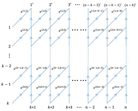
Figure 2: The planar network $N(\mathbf{x})$. Vertical edges have weight 1.

It has $n$ sources labeled $1,\dots,n$ and $n-k$ sinks labeled $1^{\prime},\dots,(n-k)^{\prime}$. Define the weight of a path to be the product of the weights of the edges in the path. Let $M(\mathbf{x})$ be an $n\times(n-k)$ matrix associated to the network $N(\mathbf{x})$, such that whose $(i,j)$-entry is the sum of the weights of all paths from source $i$ to sink $j^{\prime}$.

Example 17

In the case of $n=4$ and $\mathbf{x},\mathbf{y},\mathbf{z}$ for $\overline{\mathbb{Y}}_{k=1,2,3}$ these matrices look like

$$M(\mathbf{x})=\begin{pmatrix}x^{(1,1)}&0&0\\ 1&x^{(1,2)}&0\\ 0&1&x^{(1,3)}\\ 0&0&1\end{pmatrix},\quad M(\mathbf{y})=\begin{pmatrix}y^{(1,1)}&0\\ y^{(2,2)}&y^{(1,2)}y^{(2,2)}\\ 1&y^{(1,2)}+y^{(2,3)}\\ 0&1\end{pmatrix},$$

and

$$M(\mathbf{z})=\begin{pmatrix}z^{(1,1)}\\ z^{(2,2)}\\ z^{(3,3)}\\ 1\end{pmatrix}.$$

These matrices are given by the planar networks in Figure 3.

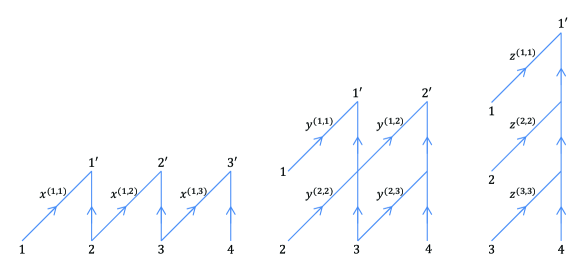
Figure 3: The planar networks $N(\mathbf{x}),N(\mathbf{y}),N(\mathbf{z})$ for the matrices $M(\mathbf{x}),M(\mathbf{y}),M(\mathbf{z})$.

Let $\overline{\Theta}_{n-k}(\mathbf{x})$ be the $n-k$ dimensional subspace of ${\mathbb{C}}^{n}$ spanned by the columns of $M(\mathbf{x})$, which is regarded as a point lies in the Grassmannian variety ${\rm Gr}(n-k,n)$. This notation implies that there is a map $\overline{\Theta}_{n-k}:\overline{\mathbb{Y}}_{k}\rightarrow{\rm Gr}(n-k,n)$, that is basically identical to the one which is called the Gelfand-Tsetlin parametrization of ${\rm Gr}(n-k,n)\times{\mathbb{C}}^{\times}$ in [2, 3].

It is known that the positivity of the Pl$\ddot{\rm u}$cker coordinates (Corollary 4.15 of [2]) holds, which tells that for all $I\in{[n]\choose n-k}$, $P_{I}(\overline{\Theta}_{n-k}(\mathbf{x}))$ is a non-zero (homogeneous) polynomial in the quantities $x^{(i,j)}$ with non-negative integer coefficients. For the currently using setup where we are dealing with only positive real parameters and variables, this implies that for any $\mathbf{x}\in\overline{\mathbb{Y}}_{k}$ every $P_{I}(\overline{\Theta}_{n-k}(\mathbf{x}))$ takes its value in ${\mathbb{R}}_{>0}$. In other words, $\overline{\Theta}_{n-k}(\mathbf{x})$ is a point lies in the totally positive Grassmannian ${\rm Gr}(n-k,n)_{>0}\subset{\rm Gr}(n-k,n)$ [18]. Moreover, the map $\overline{\Theta}_{n-k}$ is a bijection between $\overline{\mathbb{Y}}_{k}$ and ${\rm Gr}(n-k,n)_{>0}$. In fact, for $M\in{\rm Gr}(n-k,n)_{>0}$ its inverse image $\mathbf{x}=(x^{(i,j)})_{(i,j)\in R_{k}}=(\overline{\Theta}_{n-k})^{-1}(M)\in\overline{\mathbb{Y}}_{k}$ is given by the following formula (Proposition 4.3 of [2])

$$x^{(i,i)}=\frac{P_{J_{i,i}}(M)}{P_{J_{i+1,i}}(M)}\quad\mbox{or}\quad x^{(i,j)}=\frac{P_{J_{i,j}}(M)P_{J_{i+1,j-1}}(M)}{P_{J_{i+1,j}}(M)P_{J_{i,j-1}}(M)},$$ (76)

for $j\in[i+1,i+n-k-1]$. Here we used the notation for the basic subsets $J_{i,j}:=[i,j]\cup[k+j-i+2,n]\in{[n]\choose n-k}$.

Let $g^{(n-k)}(\mathbf{x},l;\lambda)$ denote an $n\times n$ matrix that is introduced in [2] to define the unipotent crystal map. The elements in the $(i,j)$ position of this matrix are defined by

$$g^{(n-k)}(\mathbf{x},l;\lambda)_{ij}=c_{ij}\frac{P_{[j-n+k+1,j-1]\cup\{i\}}(\overline{\Theta}_{n-k}(\mathbf{x}))}{P_{[j-n+k,j-1]}(\overline{\Theta}_{n-k}(\mathbf{x}))},\quad c_{ij}=\begin{cases}1&\mbox{if }j\leq n-k,\\ l&\mbox{if }j>n-k\mbox{ and }i\geq j,\\ \lambda&\mbox{if }j>n-k\mbox{ and }i<j.\end{cases}$$

Example 18

For the $\mathbf{x},\mathbf{y},\mathbf{z}$ in Example 17 for $n=4$ and $\overline{\mathbb{Y}}_{k=1,2,3}$, we have

$$g^{(3)}(\mathbf{x},l;\lambda)=\begin{pmatrix}\frac{P_{134}}{P_{234}}&0&0&\lambda\\ 1&\frac{P_{124}}{P_{134}}&0&0\\ 0&1&\frac{P_{123}}{P_{124}}&0\\ 0&0&1&l\frac{P_{234}}{P_{123}}\end{pmatrix}=\begin{pmatrix}x^{(1,1)}&0&0&\lambda\\ 1&x^{(1,2)}&0&0\\ 0&1&x^{(1,3)}&0\\ 0&0&1&x^{(1,4)}\end{pmatrix},$$

$$g^{(2)}(\mathbf{y},l;\lambda)=\begin{pmatrix}\frac{P_{14}}{P_{34}}&0&\lambda&\lambda\frac{P_{13}}{P_{23}}\\ \frac{P_{24}}{P_{34}}&\frac{P_{12}}{P_{14}}&0&\lambda\\ 1&\frac{P_{13}}{P_{14}}&l\frac{P_{23}}{P_{12}}&0\\ 0&1&l\frac{P_{24}}{P_{12}}&l\frac{P_{34}}{P_{23}}\end{pmatrix}=\begin{pmatrix}y^{(1,1)}&0&\lambda&\lambda\frac{y^{(1,1)}(y^{(1,2)}+y^{(2,3)})}{y^{(2,2)}y^{(2,3)}}\\ y^{(2,2)}&y^{(1,2)}y^{(2,2)}&0&\lambda\\ 1&y^{(1,2)}+y^{(2,3)}&y^{(1,3)}y^{(2,3)}&0\\ 0&1&y^{(1,3)}&y^{(2,4)}\end{pmatrix},$$

and

$$g^{(1)}(\mathbf{z},l;\lambda)=\begin{pmatrix}\frac{P_{1}}{P_{4}}&\lambda&\lambda\frac{P_{1}}{P_{2}}&\lambda\frac{P_{1}}{P_{3}}\\ \frac{P_{2}}{P_{4}}&l\frac{P_{2}}{P_{1}}&\lambda&\lambda\frac{P_{2}}{P_{3}}\\ \frac{P_{3}}{P_{4}}&l\frac{P_{3}}{P_{1}}&l\frac{P_{3}}{P_{2}}&\lambda\\ 1&l\frac{P_{4}}{P_{1}}&l\frac{P_{4}}{P_{2}}&l\frac{P_{4}}{P_{3}}\end{pmatrix}=\begin{pmatrix}z^{(1,1)}&\lambda&\lambda\frac{z^{(1,1)}}{z^{(2,2)}}&\lambda\frac{z^{(1,1)}}{z^{(3,3)}}\\ z^{(2,2)}&z^{(1,2)}z^{(2,2)}&\lambda&\lambda\frac{z^{(2,2)}}{z^{(3,3)}}\\ z^{(3,3)}&z^{(1,2)}z^{(3,3)}&z^{(2,3)}z^{(3,3)}&\lambda\\ 1&z^{(1,2)}&z^{(2,3)}&z^{(3,4)}\end{pmatrix}.$$

Note that the first $n-k$ columns of $g^{(n-k)}(\mathbf{x},l;\lambda)$ coincide with those of the matrix $M(\mathbf{x})$.

Several properties of the matrix $g^{(n-k)}(\mathbf{x},l;\lambda)$ presented in [3] (in our notations) are listed as follows.

Proposition 19 ([3]: Proposition 3.17 and Corollary 3.18)

Let $(\mathbf{x},l)\in\mathbb{Y}_{k},A=g^{(n-k)}(\mathbf{x},l;\lambda)$, and $B\in{\rm M}_{n}({\mathbb{C}}[\lambda,\lambda^{-1}])$.

1. The first $n-k$ columns of $A$ span the subspace $\overline{\Theta}_{n-k}(\mathbf{x})$.

2. The matrix $A|_{\lambda=(-1)^{n-k-1}l}$ has rank $n-k$.

3. The determinant of $A$ is $(l+(-1)^{n-k}\lambda)^{k}$.

4. The first $n-k$ columns of $A\cdot B|_{\lambda=(-1)^{n-k-1}l}$ are contained in the subspace $\overline{\Theta}_{n-k}(\mathbf{x})$.

Now we consider the following matrix equation

$$g^{(n-1)}(\mathbf{b},s;\lambda)g^{(n-k)}(\mathbf{a},l;\lambda)=g^{(n-k)}(\mathbf{a}^{\prime},l;\lambda)g^{(n-1)}(\mathbf{b}^{\prime},s;\lambda).$$ (77)

Proposition 20

For any $s,l\in{\mathbb{R}}_{>0}$ and $(\mathbf{b},\mathbf{a})\in\overline{\mathbb{Y}}_{1}\times\overline{\mathbb{Y}}_{k}$, there is a unique solution $(\mathbf{a}^{\prime},\mathbf{b}^{\prime})\in\overline{\mathbb{Y}}_{k}\times\overline{\mathbb{Y}}_{1}$ to the matrix equation (77).

Proof. Besides differences of the notations, an explicit expression for a solution to (77) is available in section 7.1 of [3], where the map that sends $(\mathbf{b},\mathbf{a})$ to $(\mathbf{a}^{\prime},\mathbf{b}^{\prime})$ is denoted by $\Theta R$. It remains to prove the uniqueness of the solution. Suppose there are two solutions $(\mathbf{a}^{\prime},\mathbf{b}^{\prime})$ and $(\mathbf{a}^{\prime\prime},\mathbf{b}^{\prime\prime})$, hence

$$g^{(n-k)}(\mathbf{a}^{\prime},l;\lambda)g^{(n-1)}(\mathbf{b}^{\prime},s;\lambda)=g^{(n-k)}(\mathbf{a}^{\prime\prime},l;\lambda)g^{(n-1)}(\mathbf{b}^{\prime\prime},s;\lambda).$$ (78)

Set $\lambda=(-1)^{n-k-1}l$ in the equation (77). By applying item $(iv)$ of Proposition 19 on the right hand side, we see that the first $n-k$ columns of both sides of the equation are contained in the $(n-k)$-dimensional subspace $\overline{\Theta}_{n-k}(\mathbf{a}^{\prime})$, and also in $\overline{\Theta}_{n-k}(\mathbf{a}^{\prime\prime})$ by (78). On the other hand, one observes that the bottom left $(n-k)\times(n-k)$ submatrix of the left hand side of the equation (77) is independent of $\lambda$, and its determinant is given by the geometric coenergy function (Corollary 7.3 of [3]),

$$E(\mathbf{b},\mathbf{a}) =\Delta_{[k+1,n],[n-k]}(g^{(n-1)}(\mathbf{b},s;\bullet)g^{(n-k)}(\mathbf{a},l;\bullet))$$

$$=\sum_{m=0}^{n-k}a^{(k,k)}a^{(k,k+1)}\cdots a^{(k,k+m-1)}b^{(1,k+m+1)}b^{(1,k+m+2)}\cdots b^{(1,n)}.$$ (79)

Since this quantity does not vanish, the first $n-k$ columns of both sides of equation (77) always have full rank. (This is true even if we set $s=l$ and $k$ is odd, hence the matrix $g^{(n-1)}(\mathbf{b},s;(-1)^{n-k-1}s)$ is not invertible and has rank $n-1$.) Therefore we have $\overline{\Theta}_{n-k}(\mathbf{a}^{\prime})=\overline{\Theta}_{n-k}(\mathbf{a}^{\prime\prime})$, and then $\overline{\Theta}_{n-k}(\mathbf{b}^{\prime})=\overline{\Theta}_{n-k}(\mathbf{b}^{\prime\prime})$ by equation (78) . Since the map $\overline{\Theta}_{n-k}$ gives a bijection between $\overline{\mathbb{Y}}_{k}$ and ${\rm Gr}(n-k,n)_{>0}$, we have the desired result. $\Box$

Based on this proposition, define $R^{(s,l)}:\overline{\mathbb{Y}}_{1}\times\overline{\mathbb{Y}}_{k}\rightarrow\overline{\mathbb{Y}}_{k}\times\overline{\mathbb{Y}}_{1}$ to be a rational map given by $R^{(s,l)}:(\mathbf{b},\mathbf{a})\mapsto(\mathbf{a}^{\prime},\mathbf{b}^{\prime})$. This is the geometric $R$-matrix in the present case.

3.2.2 Prerequisites for the Perron-Frobenius theorem.

For any $\mathbf{x}\in\overline{\mathbb{Y}}_{k}$ let $\vec{P}(\mathbf{x})$ be an ${n\choose k}$-component vector defined by

$$\vec{P}(\mathbf{x})=\left(\frac{P_{I}(\overline{\Theta}_{n-k}(\mathbf{x}))}{P_{[k+1,n]}(\overline{\Theta}_{n-k}(\mathbf{x}))}\right)_{I\in{[n]\choose n-k}},$$ (80)

where the indices are assumed to be in lexicographic order as in (57). Then we see that its last element is always normalized to be one.

By using the formula (76) one can recover all the elements of $\mathbf{x}=(x^{(i,j)})_{(i,j)\in R_{k}}\in\overline{\mathbb{Y}}_{k}$ from the elements of the vector $\vec{P}(\mathbf{x})$. Based on this fact, we can generalize Lemma 13 to the following:

Lemma 21

Let $R^{(s,l)}(\mathbf{b},\mathbf{a})=(\mathbf{a}^{\prime},\mathbf{b}^{\prime})$. Then the elements of $\mathbf{a}^{\prime}\in\overline{\mathbb{Y}}_{k}$ are determined by the following relation

$$\vec{P}(\mathbf{a}^{\prime})=\frac{1}{E(\mathbf{b},\mathbf{a})}\mathsf{C}_{n-k}(g^{(n-1)}(\mathbf{b},s;(-1)^{n-k-1}l))\vec{P}(\mathbf{a}),$$ (81)

where $\mathsf{C}_{n-k}$ denotes the $(n-k)$-th contravariant alternating tensor representation (57), and $E(\mathbf{b},\mathbf{a})$ is the geometric coenergy function (79).

Proof. By Frieden’s definition of the geometric $R$-matrix ((5.1) of [3]), we have $\overline{\Theta}_{n-k}(\mathbf{a}^{\prime})=g^{(n-1)}(\mathbf{b},s;(-1)^{n-k-1}l)\cdot\overline{\Theta}_{n-k}(\mathbf{a})$, where the meaning of $\cdot$ in the right hand side was given in section 1.3. As a matrix representative of $\overline{\Theta}_{n-k}(\mathbf{a}^{\prime})$, define $\tilde{M}(\mathbf{a}^{\prime})$ to be an $n\times(n-k)$ matrix given by $\tilde{M}(\mathbf{a}^{\prime})=g^{(n-1)}(\mathbf{b},s;(-1)^{n-k-1}l)M(\mathbf{a})$. Then we have

$$\frac{P_{I}(\overline{\Theta}_{n-k}(\mathbf{a}^{\prime}))}{P_{J}(\overline{\Theta}_{n-k}(\mathbf{a}^{\prime}))}=\frac{\Delta_{I,[n-k]}(\tilde{M}(\mathbf{a}^{\prime}))}{\Delta_{J,[n-k]}(\tilde{M}(\mathbf{a}^{\prime}))},$$ (82)

for any $(n-k)$-subsets $I,J$ of $[n]$. On the other hand, by applying the Cauchy-Binet formula to the definition of $\tilde{M}(\mathbf{a}^{\prime})$ we have

$$\Delta_{I,[n-k]}(\tilde{M}(\mathbf{a}^{\prime})) =\sum_{J\in{[n]\choose n-k}}\Delta_{I,J}(g^{(n-1)}(\mathbf{b},s;(-1)^{n-k-1}l))\Delta_{J,[n-k]}(M(\mathbf{a}))$$

$$=\Delta_{I,[n-k]}(g^{(n-1)}(\mathbf{b},s;(-1)^{n-k-1}l)g^{(n-k)}(\mathbf{a},l;\bullet)),$$ (83)

where we used the fact that the first $n-k$ columns of $g^{(n-k)}(\mathbf{a},l;\lambda)$ coincide with those of the matrix $M(\mathbf{a})$. Therefore by setting $I=[k+1,n]$ we have $\Delta_{[k+1,n],[n-k]}(\tilde{M}(\mathbf{a}^{\prime}))=E(\mathbf{b},\mathbf{a})$. By using this identity and the fact that the bottom left $(n-k)\times(n-k)$ submatrix of $M(\mathbf{a})$ is upper uni-triangular, we can write the first equality of (83) as

$$\frac{\Delta_{I,[n-k]}(\tilde{M}(\mathbf{a}^{\prime}))}{\Delta_{[k+1,n],[n-k]}(\tilde{M}(\mathbf{a}^{\prime}))}=\frac{1}{E(\mathbf{b},\mathbf{a})}\sum_{J\in{[n]\choose n-k}}\Delta_{I,J}(g^{(n-1)}(\mathbf{b},s;(-1)^{n-k-1}l))\frac{\Delta_{J,[n-k]}(M(\mathbf{a}))}{\Delta_{[k+1,n],[n-k]}(M(\mathbf{a}))}.$$

By (82), this is the identity which we wanted to prove. $\Box$

In what follows we omit the superscript of $g$ in the case of $k=1$, hence $g(\mathbf{x},s;\lambda)=g^{(n-1)}(\mathbf{x},s;\lambda)$ in agreement with the notation which we defined in (55). Returning to the notations in the previous subsection, let $(\mathbf{x},s)$ denote an element of $\mathbb{Y}_{1}=({\mathbb{R}}_{>0})^{n-1}\times{\mathbb{R}}_{>0}$ with $\mathbf{x}=(x^{(1)},\dots,x^{(n-1)})$, and set $x^{(n)}:=s/(x^{(1)}\cdots x^{(n-1)})$. Consider the matrix $\mathsf{C}_{r}(g(\mathbf{x},s;\lambda))$ given by (57), the $r$-th contravariant alternating tensor representation of $g(\mathbf{x},s;\lambda)$. Note that the latter matrix has a network representation [2, 3] as in Figure 4. Denote such a network by $\mathcal{N}_{0}$.

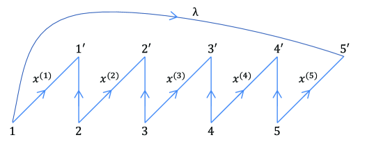
Figure 4: An example of the network representation of the matrix $g(\mathbf{x},s;\lambda)$ for $n=5$ case. Vertical edges have weight 1.

We say that a matrix is positive if all its elements are positive real numbers. In order to use the Perron-Frobenious theorem to define our system, we need to prove:

Proposition 22

For any $\mathbf{x}\in({\mathbb{R}}_{>0})^{n-1}$, $s,l\in{\mathbb{R}}_{>0}$ and $1\leq r\leq n-1$, some power of $\mathsf{C}_{r}(g(\mathbf{x},s;(-1)^{r-1}l))$ is a positive matrix.

Proof. It suffices to show that there exists a positive integer $K$ such that $\Delta_{I,J}(g(\mathbf{x},s;(-1)^{r-1}l)^{K})>0$ for any $I,J\in{[n]\choose r}$. We begin with the fact that the matrix $g(\mathbf{x},s;\lambda)^{K}$ is represented by a planar network $\mathcal{N}$ that is given by stacking the network $\mathcal{N}_{0}$ for the matrix $g(\mathbf{x},s;\lambda)$ up to $K$ times. See Figure 5 for an example of $\mathcal{N}$ . By the Lindstr$\ddot{\rm o}$m Lemma (See, for example Proposition 4.5 of [2]), such a minor determinant is expressed as

$$\Delta_{I,J}(g(\mathbf{x},s;(-1)^{r-1}l)^{K})=\sum_{\mathcal{F}=(p_{a};\sigma):I\rightarrow J}{\rm sgn}(\sigma){\rm wt}(\mathcal{F}),$$ (84)

where the sum is over vertex-disjoint paths (i.e. no two of the paths share a vertex) from $I=\{i_{1}<\dots<i_{r}\}$ to $J=\{j_{1}<\dots<j_{r}\}$ on the network $\mathcal{N}$ with $\lambda=(-1)^{r-1}l$, and $\mathcal{F}=(p_{a};\sigma)$ is a collection of $r$ paths $p_{1},\dots,p_{r}$ such that $p_{a}$ starts at source $i_{a}$ and ends at sink $j^{\prime}_{\sigma(a)}$, for some permutation $\sigma\in S_{r}$. The weight of $\mathcal{F}$ is defined as ${\rm wt}(\mathcal{F})=\prod_{a=1}^{r}{\rm wt}(p_{a})$, where ${\rm wt}(p_{a})$ is the weight of path $p_{a}$.

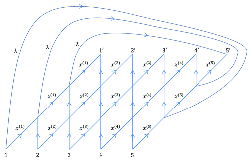
Figure 5: A three times stack of the network representation of the matrix $g(\mathbf{x},s;\lambda)$ for $n=5$ case.

First we show that for sufficiently large $K$, there exists at least one collection of vertex-disjoint paths from $I$ to $J$ for any $I,J\in{[n]\choose r}$.

1. Suppose the elements of both $I$ and $J$ are consecutive mod $n$. Let all the paths starting from the edges labeled by $I$ go vertically upward on the network. Here we also regard the edges with weight $\lambda$ as vertical ones. Then they will arrive at the edges labeled by $J$ in a finite step, if $K$ is sufficiently large.

2. Suppose $I=I_{1}\sqcup I_{2}$, where the elements of both $I_{1}$ and $I_{2}$ are consecutive mod $n$, and there is a gap between them. Let all the paths starting from the edges labeled by $I_{1}$ go diagonally upward, while those from the edges labeled by $I_{2}$ go vertically upward. In a finite step, a merger will occur. That is, they will arrive at a collection of mod $n$ consecutive edges on a common horizontal level.

3. Suppose $I$ has more than 2 consecutive (mod $n$) subsets. Let all the paths starting from the edges labeled by one of the subsets go diagonally upward, while those from the edges labeled by the other subsets go vertically upward, until a merger will occur. Then by repeating this procedure we will come to the situation in (ii). This together with the result in (i) is proving that for sufficiently large $K$ there exists at least one collection of vertex-disjoint paths from $I$ to $[r]$ for any $I\in{[n]\choose r}$.

4. In the same way, we can show that for sufficiently large $K$, there exists at least one collection of vertex-disjoint paths from $[r]$ to $J$ for any $J\in{[n]\choose r}$.

5. By combining (iii) and (iv), we obtain the result which we wanted to show.

Now we show that for any collection of vertex-disjoint paths $\mathcal{F}=(p_{a};\sigma)$ from $I$ to $J$, the summand ${\rm sgn}(\sigma){\rm wt}(\mathcal{F})$ in the expression (84) is positive. Because of the vertex-disjoint condition, any $\sigma\in S_{r}$ must be either a cyclic shift of the elements of $[r]$ or the identity map. When going upward on the network along the collection of paths $\mathcal{F}$, an elementary cyclic shift $\{1,2,\dots,r\}\rightarrow\{2,\dots,r,1\}$ may occur within one unit of the stack. In that case, the ${\rm sgn}(\sigma)$ is multiplied by $(-1)^{r-1}$, while an edge with weight $\lambda=(-1)^{r-1}l$ is picked up for the paths $\mathcal{F}$. As a result, the summand ${\rm sgn}(\sigma){\rm wt}(\mathcal{F})$ is always positive. The proof is completed. $\Box$

Recall the definition of a Lax matrix $\mathcal{L}(|\mathbf{b}\rangle;\lambda)$ in (73). Then one easily sees that an obvious extension of Proposition 22 is the following:

Corollary 23

For any $|\mathbf{b}\rangle=(\mathbf{b}_{1},\dots,\mathbf{b}_{L})\in({\mathbb{R}}_{>0})^{L(n-1)}$, $s,l\in{\mathbb{R}}_{>0}$ and $1\leq r\leq n-1$, some power of $\mathsf{C}_{r}(\mathcal{L}(|\mathbf{b}\rangle;(-1)^{r-1}l))$ is a positive matrix.

By the Perron-Frobenius theorem, this corollary implies that there exists a positive eivenvector of the matrix $\mathsf{C}_{r}(\mathcal{L}(|\mathbf{b}\rangle;(-1)^{r-1}l))$ and it is unique up to a scalar multiple.

3.2.3 Definition of the dynamical system.

In order to define the time evolutions by carriers of “rectangular tableaux”, we first show the following:

Lemma 24

Let $A=\mathcal{L}(|\mathbf{b}\rangle;(-1)^{n-k-1}l)$. Then the Perron-Frobenius eivenvector $\vec{\xi}_{\rm PF}$ of $\mathsf{C}_{n-k}(A)$ determines a unique point in ${\rm Gr}(n-k,n)_{>0}$.

Proof. Fix an arbitrary chosen $M_{0}\in{\rm Gr}(n-k,n)_{>0}$. By using the same argument in the proof of Proposition 20, we can define a sequence of $(n-k)$-dimensional subspaces $M_{0},M_{1},\dots\in{\rm Gr}(n-k,n)_{>0}$ recursively by the relation $M_{i}=A\cdot M_{i-1}$. Then by using the Cauchy-Binet formula and a consequence of the Perron-Frobenius theorem, we have $\lim_{i\rightarrow\infty}(P_{I}(M_{i}))_{I\in{[n]\choose n-k}}=\lim_{i\rightarrow\infty}\mathsf{C}_{n-k}(A)^{i}(P_{I}(M_{0}))_{I\in{[n]\choose n-k}}=\vec{\xi}_{\rm PF}$ up to a scalar multiple. Since the closure (in the Hausdorff topology) of a totally positive Grassmannian ${\rm Gr}(n-k,n)_{>0}$ is a totally nonnegative Grassmannian ${\rm Gr}(n-k,n)_{\geq 0}$ (Theorem 3.6 of [18]), this implies that there is a limiting point $M=\lim_{i\rightarrow\infty}M_{i}\in{\rm Gr}(n-k,n)_{\geq 0}$. Then since $(P_{I}(M))_{I\in{[n]\choose n-k}}=\vec{\xi}_{\rm PF}$ is a positive vector, this unique point $M$ actually lies in ${\rm Gr}(n-k,n)_{>0}$. $\Box$

Remark 25

Since the Pl$\ddot{u}$cker coordinates of every point in a Grassmannian must satisfy the Grassmann-Pl$\ddot{u}$cker relations (See, for example Proposition 3.2 of [2]), a positive vector with arbitrary chosen ${n\choose k}$ components does not necessarily determines a point in ${\rm Gr}(n-k,n)_{>0}$.

Recall that $R^{(s,l)}:\overline{\mathbb{Y}}_{1}\times\overline{\mathbb{Y}}_{k}\rightarrow\overline{\mathbb{Y}}_{k}\times\overline{\mathbb{Y}}_{1}$ is the rational map given by the matrix equation (77). As in the totally one-row tableaux case, we define $R_{i}^{(s,l)}$ and $\mathcal{R}^{(s,l)}=R_{1}^{(s,l)}\circ\cdots\circ R_{L}^{(s,l)}$ to be maps which are now from $(\overline{\mathbb{Y}}_{1})^{i}\times\overline{\mathbb{Y}}_{k}\times(\overline{\mathbb{Y}}_{1})^{L-i}$ to $(\overline{\mathbb{Y}}_{1})^{i-1}\times\overline{\mathbb{Y}}_{k}\times(\overline{\mathbb{Y}}_{1})^{L-i+1}$, and from $(\overline{\mathbb{Y}}_{1})^{L}\times\overline{\mathbb{Y}}_{k}$ to $\overline{\mathbb{Y}}_{k}\times(\overline{\mathbb{Y}}_{1})^{L}$ respectively. Given an arbitrary $(\mathbf{b}_{1},\dots,\mathbf{b}_{L},\mathbf{v})\in(\overline{\mathbb{Y}}_{1})^{L}\times\overline{\mathbb{Y}}_{k}$, let $\mathcal{R}^{(s,l)}(\mathbf{b}_{1},\dots,\mathbf{b}_{L},\mathbf{v})=(\mathbf{v}_{1},\mathbf{b}^{\prime}_{1},\dots,\mathbf{b}^{\prime}_{L})$. It is depicted by the same diagram (67) but now $\mathbf{v}_{i}$’s are the elements of $\overline{\mathbb{Y}}_{k}=({\mathbb{R}}_{>0})^{k(n-k)}$,

      (85)

Once again, by regarding the $\mathbf{b}_{i}$’s also as parameters, we consider an algebraic equation $\mathbf{v}=\mathbf{v}_{1}$ for the unknown $\mathbf{v}$ that assures the system of having a periodic boundary condition. Then we have:

Proposition 26

For any $s,l\in{\mathbb{R}}_{>0}$ and $|\mathbf{b}\rangle=(\mathbf{b}_{1},\dots,\mathbf{b}_{L})\in(\overline{\mathbb{Y}}_{1})^{L}$, there is a unique positive real solution $\mathbf{v}\in\overline{\mathbb{Y}}_{k}=({\mathbb{R}}_{>0})^{k(n-k)}$ to the equation $\mathbf{v}=\mathbf{v}_{1}$.

Proof. Let $A=\mathcal{L}(|\mathbf{b}\rangle;(-1)^{n-k-1}l)$. By repeated use of Lemma 21 we have

$$\mathsf{C}_{n-k}(A)\vec{P}(\mathbf{v})=E(\mathbf{b}_{L},\mathbf{v})E(\mathbf{b}_{L-1},\mathbf{v}_{L})\cdots E(\mathbf{b}_{1},\mathbf{v}_{2})\vec{P}(\mathbf{v}_{1}),$$ (86)

where $\mathbf{v}_{i}$’s are those determined by the diagram (85).

(Uniqueness.) Suppose there exist positive real solutions to the equation $\mathbf{v}=\mathbf{v}_{1}$. From (86) we see that for any such solution $\mathbf{v}\in\overline{\mathbb{Y}}_{k}$ it is necessary for $\vec{P}(\mathbf{v})$ to be a positive eigenvector of the matrix $\mathsf{C}_{n-k}(A)$. By Lemma 24 there is a unique $M\in{\rm Gr}(n-k,n)_{>0}$ such that $(P_{I}(M))_{I\in{[n]\choose n-k}}$ is the Perron-Frobenius eivenvector of the matrix $\mathsf{C}_{n-k}(A)$. Therefore, if any such solution $\mathbf{v}\in\overline{\mathbb{Y}}_{k}$ exists, then it must be equal to the unique one given from this $M$ by using the formula (76), because the map $\overline{\Theta}_{n-k}$ is a bijection between $\overline{\mathbb{Y}}_{k}$ and ${\rm Gr}(n-k,n)_{>0}$.

(Existence.) Equation (86) is valid for any $\mathbf{v}\in\overline{\mathbb{Y}}_{k}$ so in particular for the $\mathbf{v}$ obtained from the above mentioned unique $M\in{\rm Gr}(n-k,n)_{>0}$. On the other hand, for this $\mathbf{v}$ we also have

$$\mathsf{C}_{n-k}(A)\vec{P}(\mathbf{v})=E^{(k)}_{l}\vec{P}(\mathbf{v})$$ (87)

where $E^{(k)}_{l}$ is the dominant eigenvalue of the matrix $\mathsf{C}_{n-k}(A)$. By equating the right hand side of equation (86) with that of (87), and noting that the last element of the vector $\vec{P}(\mathbf{x})$ defined in (80) is always one for any $\mathbf{x}\in\overline{\mathbb{Y}}_{k}$, we see that this $\mathbf{v}$ is indeed a solution to the algebraic equation $\mathbf{v}=\mathbf{v}_{1}$. $\Box$

By combining the claims in Remark 14 and Proposition 26 we have the following:

Theorem 27

For any $s,l\in{\mathbb{R}}_{>0}$ and $(\mathbf{b}_{1},\dots,\mathbf{b}_{L})\in({\mathbb{R}}_{>0})^{L(n-1)}$, there is a unique positive real solution $(\mathbf{v},\mathbf{b}^{\prime}_{1},\dots,\mathbf{b}^{\prime}_{L})\in({\mathbb{R}}_{>0})^{k(n-k)}\times({\mathbb{R}}_{>0})^{L(n-1)}$ to the following matrix equation

$$g(\mathbf{b}_{1},s;\lambda)\cdots g(\mathbf{b}_{L},s;\lambda)g^{(n-k)}(\mathbf{v},l;\lambda)=g^{(n-k)}(\mathbf{v},l;\lambda)g(\mathbf{b}^{\prime}_{1},s;\lambda)\cdots g(\mathbf{b}^{\prime}_{L},s;\lambda).$$ (88)

Denote this unique positive real $\mathbf{v}$ by $\mathbf{v}=\mathbf{u}_{l}^{(k)}=\mathbf{u}_{l}^{(k)}(|\mathbf{b}\rangle)\in\overline{\mathbb{Y}}_{k}$. Define $T^{(k)}_{l}:(\overline{\mathbb{Y}}_{1})^{L}\rightarrow(\overline{\mathbb{Y}}_{1})^{L}$ to be a map given by

$$T^{(k)}_{l}(\mathbf{b}_{1},\dots,\mathbf{b}_{L})=(\mathbf{b}^{\prime}_{1},\dots,\mathbf{b}^{\prime}_{L}),$$ (89)

where the right hand side is determined by the relation $\mathcal{R}^{(s,l)}(\mathbf{b}_{1},\dots,\mathbf{b}_{L},\mathbf{u}_{l}^{(k)})=(\mathbf{u}_{l}^{(k)},\mathbf{b}^{\prime}_{1},\dots,\mathbf{b}^{\prime}_{L})$. In the same way as in the totally one-row tableaux case, we call this map a time evolution, and $\mathbf{u}_{l}^{(k)}=\mathbf{u}_{l}^{(k)}(|\mathbf{b}\rangle)$ a carrier for the state $|\mathbf{b}\rangle=(\mathbf{b}_{1},\dots,\mathbf{b}_{L})$ associated with $T^{(k)}_{l}$. This time evolution defines so far the most general case of the closed geometric crystal chain.

Once again, any homogeneous state is a fixed point of this dynamical system. To verify this claim, consider the result of Proposition 26 for the one site $L=1$ case. Then by using the explicit expression for the geometric $R$-matrix in [3], we have $\mathbf{b}^{\prime}_{1}=\mathbf{b}_{1}$. Then the same argument in the totally one-row tableaux case leads to the required consequence.

By Theorem 27, the time evolution (89) is described by a Lax equation for the matrix (73) as

$$\mathcal{L}(T^{(k)}_{l}|\mathbf{b}\rangle;\lambda)=(g^{(n-k)}(\mathbf{u}_{l}^{(k)},l;\lambda))^{-1}\mathcal{L}(|\mathbf{b}\rangle;\lambda)g^{(n-k)}(\mathbf{u}_{l}^{(k)},l;\lambda).$$ (90)

Therefore, the conservation laws considered in section 3.1.2 are valid for any time evolutions $\{T^{(k)}_{l}\}_{1\leq k\leq n-1,l\in{\mathbb{R}}_{>0}}$. Also, since the geometric $R$-matrices satisfy the Yang-Baxter relation (Theorem 5.10(3) of [3]), the same argument in section 2.2.1 assures the commutativity of the time evolutions. That is, we have $T^{(k_{1})}_{l_{1}}\circ T^{(k_{2})}_{l_{2}}=T^{(k_{2})}_{l_{2}}\circ T^{(k_{1})}_{l_{1}}$ for any $1\leq k_{1},k_{2}\leq n-1$ and $l_{1},l_{2}\in{\mathbb{R}}_{>0}$.

3.2.4 Invertibility.

As in the $n=2$ case, every time evolution $T^{(k)}_{l}$ is invertible. An explicit expression for the inverse map $(T^{(k)}_{l})^{-1}$ is given as follows. For any $n\times n$ matrix $X=(X_{ij})_{1\leq i,j\leq n}$, let ${\rm fl}(X)$ be an $n\times n$ matrix such that whose elements in the $(i,j)$ position are given by ${\rm fl}(X)_{ij}=X_{n+1-j,n+1-i}$. Then ${\rm fl}$ is an anti-automorphism of the ring of $n\times n$ matrices.

Define $S_{l}:\overline{\mathbb{Y}}_{k}\rightarrow\overline{\mathbb{Y}}_{k}$ to be a map given by $S_{l}(\mathbf{x})=\mathbf{x}^{\prime}=(x^{\prime(i,j)})_{(i,j)\in R_{k}}$ where $x^{\prime(i,j)}=x^{(k+1-i,n+1-j)}$ for $i+1\leq j\leq i+n-k-1$, and $x^{\prime(i,i)}=l/\prod_{m=k+1-i}^{n-i}x^{(k+1-i,m)}$, for any $\mathbf{x}=(x^{(i,j)})_{(i,j)\in R_{k}}\in\overline{\mathbb{Y}}_{k}$. This map is essentially identical with the geometric Sch$\ddot{\rm u}$tzenberger involution [2, 3]. Then by the proof of Theorem 7.3 of [2] we have

$${\rm fl}\circ g^{(n-k)}(\mathbf{x},l;\lambda)=g^{(n-k)}(S_{l}(\mathbf{x}),l;\lambda).$$ (91)

When $k=1$ we sometimes write $\mathbf{x}=(x^{(1)},x^{(2)},\dots,x^{(n-1)})\in\overline{\mathbb{Y}}_{1}$ and then we have $S_{s}(\mathbf{x})=(x^{(n)},x^{(n-1)},\dots,x^{(2)})$ where $x^{(n)}=s/(x^{(1)}\cdots x^{(n-1)})$. By extending its definition, for any $|\mathbf{b}\rangle=(\mathbf{b}_{1},\dots,\mathbf{b}_{L})\in(\overline{\mathbb{Y}}_{1})^{L}$ we let $S_{s}|\mathbf{b}\rangle=(S_{s}(\mathbf{b}_{L}),\dots,S_{s}(\mathbf{b}_{1}))$. Note that the order of the elements is reversed. Since ${\rm fl}$ is an anti-automorphism we have ${\rm fl}(\mathcal{L}(|\mathbf{b}\rangle;\lambda))=\mathcal{L}(S_{s}|\mathbf{b}\rangle;\lambda).$ Therefore, by applying the anti-automorphism ${\rm fl}$ on both sides of (90) we obtain

$$\mathcal{L}(S_{s}\circ T^{(k)}_{l}|\mathbf{b}\rangle;\lambda)=g^{(n-k)}(S_{l}(\mathbf{u}_{l}^{(k)}),l;\lambda)\mathcal{L}(S_{s}|\mathbf{b}\rangle;\lambda)(g^{(n-k)}(S_{l}(\mathbf{u}_{l}^{(k)}),l;\lambda))^{-1},$$

or equivalently

$$\mathcal{L}(S_{s}|\mathbf{b}\rangle;\lambda)=(g^{(n-k)}(S_{l}(\mathbf{u}_{l}^{(k)}),l;\lambda))^{-1}\mathcal{L}(S_{s}\circ T^{(k)}_{l}|\mathbf{b}\rangle;\lambda)g^{(n-k)}(S_{l}(\mathbf{u}_{l}^{(k)}),l;\lambda).$$

By comparing with the definition of time evolution $T^{(k)}_{l}$, we see from this equation that $S_{s}|\mathbf{b}\rangle=T^{(k)}_{l}\circ S_{s}\circ T^{(k)}_{l}|\mathbf{b}\rangle$. Since $S_{s}$ is an involution and $|\mathbf{b}\rangle$ is an arbitrary element of $(\overline{\mathbb{Y}}_{1})^{L}$, we have

$$(T^{(k)}_{l})^{-1}=S_{s}\circ T^{(k)}_{l}\circ S_{s}.$$ (92)

This is the explicit expression for the inverse map.

3.2.5 Geometric lifting of the energy of paths.

We reconsider the results on the conservation laws of the closed geometric crystal chains in section 3.1.2. In order to study the characteristic polynomial of the Lax matrix (73), we present some basic properties of the contravariant alternating tensor representation (57).

Lemma 28

For any $n\times n$ upper triangular matrix $B$, the ${n\choose r}\times{n\choose r}$ matrix $\mathsf{C}_{r}(B)$ is also upper triangular.

Proof. Let $B=(b_{ij})_{1\leq i,j\leq n}$ where $b_{ij}=0$ when $i>j$. By definition, the matrix elements of $\mathsf{C}_{r}(B)$ are written as

$$\Delta_{I,J}(B)=\sum_{\sigma\in S_{r}}{\rm sgn}(\sigma)b_{i_{1},j_{\sigma(1)}}b_{i_{2},j_{\sigma(2)}}\cdots b_{i_{r},j_{\sigma(r)}},$$ (93)

for $I=\{i_{1}<i_{2}<\dots<i_{r}\}$ and $J=\{j_{1}<j_{2}<\dots<j_{r}\}$. We are to show that if $I>J$ in lexicographic order, then $\Delta_{I,J}(B)=0$. Let $q\in[r]$ be the smallest integer such that $i_{q}>j_{q}$. Choose an arbitrary permutation $\sigma\in S_{r}$. If $\sigma(q)\leq q$ then $i_{q}>j_{q}\geq j_{\sigma(q)}$, hence $b_{i_{q},j_{\sigma(q)}}=0$. Otherwise one has $\sigma(q)\geq q+1$. Then one of the $\sigma(q+1),\sigma(q+2),\dots,\sigma(r)$ is smaller than or equal to $q$. Suppose $\sigma(a)\leq q$ for $a\in[q+1,r]$. Then $i_{a}>i_{q}>j_{q}\geq j_{\sigma(a)}$, hence $b_{i_{a},j_{\sigma(a)}}=0$. Therefor, every term of the summation in (93) is zero when $I>J$. The proof is completed. $\Box$

Since any square matrix is similar to some upper triangular matrix, a consequence of this lemma is the following:

Corollary 29

Suppose a collection of complex numbers $\{\mu_{1},\ldots,\mu_{n}\}$ is the multiset [24] of eigenvalues of an $n\times n$ matrix $A\in{\rm M}_{n}({\mathbb{C}})$, in which their multiplicities are taken into account as repetitions of the elements. Then the eigenvalues of the ${n\choose r}\times{n\choose r}$ matrix $\mathsf{C}_{r}(A)\in{\rm M}_{{n\choose r}}({\mathbb{C}})$ are given by the multiset

$$\{\mu_{i_{1}}\mu_{i_{2}}\cdots\mu_{i_{r}}|1\leq i_{1}<i_{2}<\ldots<i_{r}\leq n\}.$$

Since the matrix elements of the Lax matrix (73) are polynomials of the loop parameter $\lambda$, it is legitimate to substitute an arbitrary complex number into $\lambda$. So in what follows we fix a $\lambda\in{\mathbb{C}}$. Then the characteristic polynomial of the Lax matrix $\mathcal{L}(|\mathbf{b}\rangle;\lambda)$ can be written as

$$\det(x\mathbb{I}_{n}-\mathcal{L}(|\mathbf{b}\rangle;\lambda))=\prod_{i=1}^{n}(x-\mu_{i}).$$

Since this polynomial is invariant under the time evolutions, each eigenvalue $\mu_{i}$ (that depends on $\lambda\in{\mathbb{C}}$) is a conserved quantity of the closed geometric crystal chain. For any $I=\{1\leq i_{1}<\dots<i_{n-k}\leq n\}\in{[n]\choose n-k}$, let $\mu_{I}=\mu_{i_{1}}\cdots\mu_{i_{n-k}}$. By Corollary 29 we have

$$\det\left(x\mathbb{I}_{{n\choose k}}-\mathsf{C}_{n-k}(\mathcal{L}(|\mathbf{b}\rangle;\lambda)\right)=\prod_{I\in{[n]\choose n-k}}(x-\mu_{I}).$$

Therefore, the eigenvalues of the matrix $\mathsf{C}_{n-k}(\mathcal{L}(|\mathbf{b}\rangle;\lambda)$ are also conserved quantities. In particular, the Perron-Frobenius eigenvalue of the monodromy matrix

$$\mathsf{M}_{l}^{(k)}(|\mathbf{b}\rangle):=\mathsf{C}_{n-k}(\mathcal{L}(|\mathbf{b}\rangle;(-1)^{n-k-1}l)),$$

is a positive real conserved quantity, which we denoted by $E_{l}^{(k)}$ in (87). Then we have

$$\mathsf{M}_{l}^{(k)}(|\mathbf{b}\rangle)\vec{P}(\mathbf{u}_{l}^{(k)})=E_{l}^{(k)}\vec{P}(\mathbf{u}_{l}^{(k)}).$$ (94)

By comparing this with the expression in (86) we have

$$E_{l}^{(k)}=E(\mathbf{b}_{L},\mathbf{u}_{l}^{(k)})E(\mathbf{b}_{L-1},\mathbf{v}_{L})\cdots E(\mathbf{b}_{1},\mathbf{v}_{2}),$$

where $\mathbf{v}_{i}$’s are those determined by the diagram (85) with $\mathbf{v}_{1}=\mathbf{v}=\mathbf{u}_{l}^{(k)}$. This expression with the explicit formula for the geometric coenegy functions (79) implies that the Perron-Frobenius eigenvalues $E_{l}^{(k)}$ are the geometric liftings of the energy of paths, a conserved quantity of the (generalized periodic) box-ball systems [4] (See, also [8]).

4 Summary and Discussions

In this paper we proposed a method to construct a new family of non-linear discrete integrable systems. They are thought of as a geometric lifting of the integrable cellular automata known as the generalized periodic box-ball systems. By combining the G. Frieden’s work on the geometric $R$-matrix with the Perron-Frobenious theorem, we were able to define a commuting family of time evolutions $T^{(k)}_{l}$ for any $1\leq k\leq n-1$ and $l\in{\mathbb{R}}_{>0}$ on the whole ‘phase space’ $({\mathbb{R}}_{>0})^{L(n-1)}$. In order to apply this theorem in linear algebra to our construction of the non-linear integrable systems, Lemmas 13 and 21 played an important role. These lemmas claim that, although the geometric $R$-matrix is a non-linear rational map, it can be viewed as almost a linear map provided that all its non-linearities have been pushed into a procedure of the Gelfand-Tsetlin parametrization, and also into a scalar factor called the geometric coenergy function. Underlying ideas in these lemmas are inspired by a deep insight on the property of this rational map (Remark 5.2 of [3]).

We have shown that the time evolutions are described by Lax equations, hence the conserved quantities are given by the coefficients of the characteristic polynomial of the associated Lax matrices. Equivalently, they are given as the eigenvalues of the Lax matrices, and this fact gave us a simple viewpoint that the dominant eigenvalue $E^{(k)}_{l}$ of the monodromy matrix is a geometric lifting of the energy of path (state) of the corresponding generalized periodic box-ball system. We noted this fact again here because the energy of paths is thought of as one of the most important notions in the theory of integrable systems associated with crystals, because it is related not only to the number of solitons in the cellular automata, but also to the number of strings in the combinatorial Bethe ansatz for certain integrable quantum spin chain models associated with such cellular automata [14, 15, 16, 17].

Regarding more about the dominant eigenvalue $E_{l}^{(k)}$, for any $k\in[n-1],l\in{\mathbb{R}}_{>0}$, and a given initial state, it is a constant under any time evolutions. This fact allows us to adopt an interpretation that we can regard $E_{l}^{(k)}$ as one of the constant parameters of the system along with $s$ and $l$. It also implies that for an actual realization of our dynamical system on a computer program, though there is a possible purely numerical calculation process to solve an algebraic equation for getting the dominant eigenvalue of the monodromy matrix, we need to do that only once for each initial condition and all the remaining calculation processes can be coded purely symbolic. In fact, under this interpretation, the elements of the carrier $\mathbf{u}_{l}^{(k)}$ are viewed as rational (if not subtraction-free rational) functions of $|\mathbf{b}\rangle$. This is based on the fact that the vector $\vec{P}(\mathbf{u}_{l}^{(k)})$ satisfies the system of linear equation (94) with the constant parameters $s,l,E_{l}^{(k)}$, and $\mathbf{u}_{l}^{(k)}$ is obtained from this vector by using the rational map (76). To be more precise for the former claim, let $N={n\choose k},\mathsf{M}_{l}^{(k)}(|\mathbf{b}\rangle)=(L_{i,j})_{1\leq i,j\leq N}$, and $\vec{P}(\mathbf{u}_{l}^{(k)})=(\mathcal{P}_{1},\mathcal{P}_{2},\dots,\mathcal{P}_{N-1},1)^{t}$. Then we have

$$\begin{pmatrix}L_{11}-E_{l}^{(k)}&L_{12}&\dots&L_{1,N-1}\\ L_{21}&L_{22}-E_{l}^{(k)}&\dots&L_{2,N-1}\\ \vdots&\vdots&\ddots&\vdots\\ L_{N-1,1}&\dots&L_{N-1,N-2}&L_{N-1,N-1}-E_{l}^{(k)}\end{pmatrix}\begin{pmatrix}\mathcal{P}_{1}\\ \mathcal{P}_{2}\\ \vdots\\ \mathcal{P}_{N-1}\end{pmatrix}=-\begin{pmatrix}L_{1,N}\\ L_{2,N}\\ \vdots\\ L_{N-1,N}\end{pmatrix}.$$

Therefore by the Cramer’s rule the $\mathcal{P}_{i}$s are given by rational functions of $L_{i,j}$s and $E_{l}^{(k)}$. For instance, if $n=2$ the carrier $v(=\mathbf{u}_{l}^{(1)})$ in (9) is expressed as $v=(E_{l}^{(1)}-L_{22})/L_{21}=-L_{12}/(L_{11}-E_{l}^{(1)})$.

In the case of $n=2$, we conducted a detailed study on the system. This includes an explicit list of the conserved quantities, a discussion on the continuum limit of the system to derive associated differential equations, and also on the tropicalization of the system. The latter study was done not only on the conserved quantities, but also on the equation for the periodic boundary condition (8). This result gives us an explanation for the existence of the non-evolvable states in the generalized periodic box-ball systems. That is, while equation (8) has a unique positive real solution, its tropicalized counterpart (44) does not always have a unique non-negative integer solution. We note once again that although the equation (8) itself can be tropicalized, its solution can not be tropicalized. In this sense, we admit that the closed geometric crystal chain is not literally a geometric lifting of the generalized periodic box-ball system.

In the case of general $n$, we mainly restricted ourselves to solve the problem of whether we can define, if any, time evolutions compatible with the periodic boundary condition. Now this work has been done, in future studies we would like to clarify more detailed properties of the system for the case of general $n$, such as taking a continuum limit of the system to obtain associated differential equations, and seeking an explicit formula for the tropical limit of the energy of paths and the equation for the periodic boundary condition, as we have done in the case of $n=2$. Also, there are many other remaining problems to be addressed; whether we will be able to construct soliton solutions in our systems, to give any explicit formulas to describe solutions to initial value problems, to clarify the global structure of the iso-level sets of our dynamical systems in the phase space $({\mathbb{R}}_{>0})^{L(n-1)}$, to define the action of the geometric crystal operators $e^{c}_{i}$’s on the states of our systems, and to clarify how the iso-level sets will be changed under the operations of these operators. Generalization of the states of the systems from homogeneous paths associated with only one-row tableaux to inhomogeneous paths with more general rational rectangles, may be another interesting problem.

Lastly, we give an additional discussion on the conserved quantities in the case of general $n$ in section 3.1.2. In fact, there is another way of giving them in terms of polynomials of the variables $\{b_{i}^{(j)}\}_{1\leq i\leq L,1\leq j\leq n}$ with non-negative integer coefficients. As we have seen in the proof of Proposition 22, such a minor determinant is expressed as

$$\Delta_{I,I}(\mathcal{L}(|\mathbf{b}\rangle;\lambda))=\sum_{\mathcal{F}=(p_{a};\sigma):I\rightarrow I}{\rm sgn}(\sigma){\rm wt}(\mathcal{F}),$$

where the sum is over vertex-disjoint paths from $I=\{i_{1}<\dots<i_{n-k}\}$ to itself on a certain planar network associated with the matrix $\mathcal{L}(|\mathbf{b}\rangle;\lambda)$, and $\mathcal{F}=(p_{a};\sigma)$ is a collection of $n-k$ paths $p_{1},\dots,p_{n-k}$ such that $p_{a}$ starts at source $i_{a}$ and ends at sink $i_{\sigma(a)}$, for some permutation $\sigma\in S_{n-k}$. By a similar consideration in that proof, we see that for any $m$ the coefficient of $\lambda^{m}$ in the polynomial ${\rm Tr}\mathsf{C}_{n-k}(\mathcal{L}(|\mathbf{b}\rangle;\lambda))$ is given by a polynomial of the variables $\{b_{i}^{(j)}\}_{1\leq i\leq L,1\leq j\leq n}$ with non-negative integer coefficients, multiplied by a sign factor $(-1)^{m(n-k-1)}$. Therefore, by removing this sign factor, every conserved quantity contained in ${\rm Tr}\mathsf{C}_{n-k}(\mathcal{L}(|\mathbf{b}\rangle;\lambda))$ can be expressed by a polynomial with non-negative integer coefficients. This implies that, all the conserved quantities of the closed geometric crystal chains thus obtained can be tropicalized. As in the case of $n=2$, it is fairly reasonable to expect that their tropicalization provides a collection of piecewise-linear formulas for conserved quantities of the integrable cellular automata with periodic boundary conditions in [16], and their possible extensions from single box tableaux to general one-row tableaux for the site variables in such cellular automata.

Acknowledgement. The authors thank Prof. Takashi Arai and Prof. Kazuo Hosomichi for valuable comments on the second author’s master thesis to which the present work is partially related.

References

- [1] Berenstein A and Kazhdan D 2000 Geometric and unipotent crystals Visions in Mathematics, GAFA 2000 Special Volume, Part I, eds. N. Alon, J. Bourgain, A. Connes, M. Gromov, and V. Milman, (Birkhäuser: Basel), 188–236
- [2] Frieden G 2019 Affine type geometric crystal on the Grassmannian J. Comb. Theory, Series A 167 499–563
- [3] Frieden G 2018 The geometric -matrix for affine crystals of type arXiv:1710.07243v2
- [4] Fukuda K, Okado M and Yamada Y 2000 Energy functions in box ball systems Internat. J. Modern Phys. A 15 1379–1392
- [5] Fulton W 1997 Young tableaux: with applications to representation theory, (Cambridge Univ. Press: Cambridge)
- [6] Hirota R and Tsujimoto S 1995 Conserved quantities of a class of nonlinear difference-differential equations J. Phys. Soc. Jpn. 64 3125–3127
- [7] Hirota R, Tsujimoto S and Imai T 1993 Difference scheme of soliton equations Future Directions of Nonlinear Dynamics in Physical and Biological Systems, eds. P. L. Christiansen, J. C. Elibeck and R. D. Parmentier, (Plenum Press: New York), 7–15
- [8] Inoue R, Kuniba A and Takagi T 2012 Integrable structure of box-ball systems: crystal, Bethe ansatz, ultradiscretization and tropical geometry J. Phys. A: Math. Gen. 45 073001 (63 pages)
- [9] Inoue R, Lam T and Pylyavskyy P 2019 On the cluster nature and quantization of geometric -matrices Publ. RIMS 55 25–78
- [10] Inoue R and Takenawa T 2008 Tropical spectral curves and integrable cellular automata Int. Math. Res. Not. IMRN, no. 9, rnn019
- [11] Kashiwara M 1991 On crystal bases of -analogue of universal enveloping algebras Duke Math. J. 63 465–516
- [12] Kashiwara M 1994 Crystal bases of modified quantized envoloping algebras Duke Math. J. 73 383–413
- [13] Kimijima T and Tokihiro T 2002 Initial-value problem of the discrete periodic Toda equations and its ultradiscretization Inverse Problems 18 1705–1732
- [14] Kuniba A and Sakamoto R 2008 Combinatorial Bethe ansatz and generalized periodic box-ball system Rev. Math. Phys. 20 493–527
- [15] Kuniba A Takagi T and Takenouchi A 2006 Bethe ansatz and inverse scattering transform in a periodic box-ball system Nucl. Phys. B 747 [PM] 354–397
- [16] Kuniba A and Takagi T 2010 Bethe ansatz, inverse scattering transform and tropical Riemann theta function in a periodic soliton cellular automaton for SIGMA Symmetry Integrability Geom. Methods Appl. 6, Paper 013, (52 pages)
- [17] Kuniba A and Takenouchi A 2006 Periodic cellular automata and Bethe ansatz Proceedings of 23rd International Conference “Differential Geometric Methods in Theoretical Physics” (20–26, 2005, Tianjin), eds. M.-L. Ge and W. Zhang, Nankai Tracts in Math. 10 293–302
- [18] Lam T 2016 Totally nonnegative Grassmannian and Grassmann polytopes Current Developments in Mathematics 2014, (Int. Press: Somerville MA) 51–152
- [19] Lam T and Pylyavskyy P 2011 Affine geometric crystals in unipotent loop groups Rep. Theor. 15 719–728
- [20] Lam T and Pylyavskyy P 2012 Total positivity in loop groups, I: whirls and curls Adv. Math. 230 (3) 1222–1271
- [21] Lax P D 1996 Linear Algebra, (Wiley: New York)
- [22] Satake I 1973 Senkei Daisûgaku (Linear Algebra), (Shokabo: Tokyo) [In Japanese]
- [23] Sklyanin E K 2000 Bäcklund transformations and Baxter’s -operator Integrable systems: from classical to quantum (Montreal, QC, 1999), CRM Proc. Lecture Notes 26, (American Mathematical Society, Providence, RI), 227–250
- [24] Stanley R P 1997 Enumerative Combinatorics (Vol. I). (Cambridge University Press: Cambridge)
- [25] Suris Yu B 2004 Discrete Lagrangian Models Discrete Integrable Systems, Lect. Notes Phys. 644, eds. B Grammaticos, Y Kosmann-Schwarzbach, and T Tamizhmani, (Springer: Berlin Heidelberg), 111–184
- [26] Takagi T 2009 Creation of ballot sequences in a periodic cellular automaton J. Phys. Soc. Jpn. 78 024003 (15 pages)
- [27] Takagi T 2014 Combinatorial aspects of the conserved quantities of the tropical periodic Toda lattice J. Phys. A: Math. Gen. 47 395201 (25 pages)
- [28] Takahashi D and Satsuma J 1990 A soliton cellular automaton J. Phys. Soc. Jpn. 59 no. 10, 3514–3519
- [29] Veselov A P 2005 Yang-Baxter maps: dynamical point of view Combinatorial Aspect of Integrable Systems (MSJ Memoirs vol 17) (Tokyo: Mathematical Society of Japan) 145–167
- [30] Yamada Y 2001 A birational representation of Weyl group, combinatorial -matrix and discrete Toda equation Physics and Combinatorics 2000, eds. A. N. Kirillov and N. Liskova (World Scientific, 2001) 305–319
- [31] Yoshihara D, Yura F and Tokihiro T 2003 Fundamental cycle of a periodic box-ball system J. Phys. A: Math. Gen. 36 99–121
- [32] Yura F and Tokihiro T 2002 On a periodic soliton cellular automaton J. Phys. A: Math. Gen. 35 3787–3801