Mechanism of current noise spectrum in a nonequilibirum Kondo dot system

Abstract

We systematically study the nonequilibirum Kondo mechanisms of quantum noise spectrum based on the accurate dissipaton–equation–of–motion evaluations. By comparing the noise spectra between the equilibrium and nonequilibrium cases and between the non-Kondo and Kondo regimes, we identify the nonequilibrium Kondo features in the current noise spectrum, appearing in the region of $\omega\in[-eV,eV]$. The Kondo characteristic at $\omega=\pm eV=\pm(\mu_{\rm L}-\mu_{\rm R})$ display asymmetrical upturns and remarkable peaks in $S(\omega)$ and ${\rm d}S(\omega)/{\rm d}\omega$, respectively. These features are originated from the Rabi interference of the transport current dynamics, with the Kondo oscillation frequency of $|eV|$. The minor but very distinguishable inflections, crossing over $\omega=-eV$ to $\omega=+eV$, would be related to a sort of Kondo-Fano interference between two Kondo resonances channels.

I Introduction

Shot noise of nonequilibrium quantized charge current fluctuations carries much rich information beyond the average current Bla001 ; Imr02 ; Bee0337 ; Naz03 . The study of current noise in transport through mesoscopic devices becomes a field of intensive theoretical and experimental research. Noise spectrum is the Fourier transformation of two–time current–current correlation function. The zero-frequency noise describes the steady–state fluctuations of the effective carrier charge that can be either fraction Pic97162 ; Rez99238 ; Bid09236802 or integer Koz003398 ; Lef03067002 . Noise spectrum in full frequency domain contains both static and dynamic information. It is a powerful probe to the energetics, interactions and dynamics of strongly correlated systems Ent07193308 ; Li05066803 ; Bar06017405 ; Gab08026601 ; Wab09016802 ; Liu131866 ; Jin13025044 ; Jin11053704 ; Eng04136602 ; Rot09075307 ; Yan14115411 .

Thanks to the recent advancement in on-chip detection technique, high-precision measurement of nonequilibrium current fluctuations in a Kondo quantum dot (QD) is now available at finite frequency Bas10166801 ; Bas12046802 ; Del18041412 . In the finite-frequency noise spectrum, the Kondo feature is predicted a logarithmic singularity at $\omega=\pm eV$ Moc11201303 ; Mul13245115 . One can also observe the Kondo peaks in the derivative noise to bias voltage $V$ Bas12046802 ; Del18041412 . In particular, the emissive spectrum, which is largely uncontaminated, has been studied experimentally Del18041412 and theoretically Cre18107702 , for QDs in asymmetrical coupling to reservoirs.

In this work, we will explore the nonequilibirum Kondo mechanism in the noise spectrum of the current tunneling through an Anderson impurity quantum dot. It is well-known that the equilibrium Kondo effect leads to the impurity density of state (DOS), $A(\omega)$, a resonance peak, which splits into two peaks under an applied bias voltage. The observed Kondo resonance at Fermi level is due to the formation of singlet on the QD screened by itinerant electrons from reservoirs. Away from the Kondo regime, the DOS also contains the two Hubbard resonances peaks at the single-occupation and double occupation transport resonances. That is, the DOS $A(\omega)$ reflects the structure information of the impurity system.

On the other hand, the nonequilibrium noise spectrum, $S(\omega)$, the Fourier transformation of current–current correlation function, involves not only the structure but also the transport dynamics. We will systematically investigate the nonequilibrium Kondo characteristics in both $S(\omega)$ and ${\rm d}S(\omega)/{\rm d}\omega$. The underlying mechanisms are identified, against the possible competing processes. Some details are as follows. (i) We illustrate the Kondo characteristic in both $S(\omega)$ and ${\rm d}S(\omega)/{\rm d}\omega$, with a close comparison between the equilibrium and nonequilibrium cases. The observed Kondo characteristic is related only with the Fermi energies difference between two electrodes. Namely, the applied bias voltage splits the Kondo characteristics, from the single inflection point in $S(\omega)$ and the peak ${\rm d}S(\omega){\rm d}\omega$ at $\omega=0$, into two asymmetric upturns and peaks, respectively, at around $\omega=\pm|\mu_{\rm L}-\mu_{\rm R}|=\pm eV$; (ii) By comparing the non-Kondo and Kondo regimes, we identify the nonequilibrium Kondo features in the current noise spectrum, appearing in the region of $\omega\in[-eV,eV]$. This is a type of Kondo-Fano interference, engaging both Kondo characteristics at $-eV$ and $+eV$. In contrast, the non-Kondo cotunneling process is of the anti-Stokes in nature, occurring at $-eV$ only, which rules out the interference in $\omega\in[-eV,eV]$; (iii) We establish a bridge between the nonequilibrium Kondo noise and the transient current. The observed Kondo profile around $\omega=\pm eV$ reflects the Rabi interference of the transport current dynamics and contains the information of the Kondo oscillation frequency $|eV|$; (iv) We illustrate that the emission noise Kondo feature ($\omega<0$) is often cleaner than the absorption ($\omega>0$), as the latter would be contaminated by the sequential tunneling signals.

The present study is based on the well-established dissipaton equation of motion (DEOM) approach Jin15234108 ; Yan14054105 ; Yan16110306 ; Zha18780 ; Wan20041102 . This is a nonperturbative and accurate method, having been extensively explored in the study of quantum impurity problems Jin15234108 ; Zha16237 ; Zha16204109 ; Che20297811 ; Wan20164113 ; Gon20154111 ; Jin20235144 . These include the recent noise spectrum evaluations, with the identification of Coulomb blockade assisted Rabi interference in a double-dot Aharonov-Bohm interferometer Jin20235144 .

The remainder of this paper is organized as follows. In Sec. II, we give a brief introduction of the DEOM theory and demonstrate how it evaluates the two-time current-current correlation function. In Sec. III, we demonstrate and elaborate the numerical results of the circuit current noise spectrum and the related transient circuit current. Finally, we conclude this work with Sec. IV.

II Methodology

In this section, we present a brief account on the DEOM theory and current-current correlation function. For details see References Yan14054105 ; Jin15234108 ; Yan16110306 .

Consider an electron transport setup in which an impurity system $H_{\mbox{\tiny S}}$ is sandwiched by electrode bath $h_{\mbox{\tiny B}}$, under an electric bias potential ($eV=\mu_{{\rm L}}-\mu_{{\rm R}}$) applied across the leads, $\alpha={\rm L}$ and R. The total Hamiltonian reads $H_{\rm tot}=H_{\mbox{\tiny S}}+H_{\mbox{\tiny B}}+H_{\mbox{\tiny SB}}$. The system Hamiltonian $H_{\mbox{\tiny S}}$ is arbitrary, including electron-electron interaction, given in terms of local electron creation $\hat{a}^{\dagger}_{u}$ (annihilation $\hat{a}_{u}$) operators. For instance, in the present study we consider a QD represented by the spin-$1/2$ single Anderson impurity model (SAIM) described by

$$H_{\mbox{\tiny S}}=\sum_{u=\uparrow,\downarrow}\varepsilon_{u}\hat{a}^{\dagger}_{u}\hat{a}_{u}+\frac{U}{2}\sum_{u}\hat{n}_{u}\hat{n}_{\bar{u}},$$ (1)

where the single level in the QD is characterized by a spin-degenerate energy level $\varepsilon_{\uparrow}=\varepsilon_{\downarrow}=\varepsilon$ and $\hat{n}_{u}=\hat{a}^{\dagger}_{u}\hat{a}_{u}$, with $\bar{u}$ the opposite direction of the spin index $u$.

The electrode bath is modeled as noninteracting electrons reservoirs, $H_{\mbox{\tiny B}}=\sum_{\alpha k}(\varepsilon_{\alpha k}+\mu_{\alpha})c^{\dagger}_{\alpha k}c_{\alpha k}$. Its coupling to the system assumes the standard tunneling form of

$$H_{\mbox{\tiny SB}}\!=\!\sum_{\alpha u}\left(\hat{a}^{+}_{u}\hat{F}^{-}_{\alpha u}+\hat{F}^{+}_{\alpha u}\hat{a}^{-}_{u}\right)\!=\!\sum_{\alpha u\sigma}\hat{a}^{\bar{\sigma}}_{u}\widetilde{F}^{\sigma}_{\alpha u},$$ (2)

with $\hat{F}^{-}_{\alpha u}=\sum_{k}t_{\alpha uk}c_{\alpha k}=(\hat{F}^{+}_{\alpha u})^{\dagger}$. Note that $\hat{F}^{\sigma}_{\alpha u}\hat{a}^{\bar{\sigma}}_{u}=-\hat{a}^{\bar{\sigma}}_{u}\hat{F}^{\sigma}_{\alpha u}$. For the convenience of description, we denote $\widetilde{F}^{\sigma}_{\alpha u}\equiv\bar{\sigma}\hat{F}^{\sigma}_{\alpha u}$, with $\sigma=+,-$ ($\bar{\sigma}$ is the opposite sign) identifying the creation and annihilation operators.

For the dissipaton description of bath interaction Jin15234108 ; Yan14054105 , we consider the bare-bath correlation function in the exponential decomposition form Jin08234703 ; Zhe121129 ; Zhe13086601 ; Li12266403 ; Hou15104112 ; Ye16608 ,

$$\big{\langle}\hat{F}^{\sigma}_{\alpha u}(t)\hat{F}^{\bar{\sigma}}_{\alpha v}(0)\big{\rangle}_{\mbox{\tiny B}}=\sum_{m=1}^{M}\eta^{\sigma}_{\alpha uvm}e^{-\gamma^{\sigma}_{\alpha m}t}.$$ (3)

This is realized via a sum-over-poles decomposition for the Fourier integrand of the relation $\langle\hat{F}^{\sigma}_{\alpha u}(t)\hat{F}^{\bar{\sigma}}_{\alpha v}(0)\rangle_{\mbox{\tiny B}}=\frac{1}{\pi}\int_{-\infty}^{\infty}\!\!d\omega\,e^{\sigma i(\omega+\mu_{\alpha}\!)t}\frac{J^{\sigma}_{\alpha uv}(\omega)}{1+e^{\sigma\beta\omega}}$. Here, $J^{+}_{\alpha vu}(\omega)=J^{-}_{\alpha uv}(\omega)=J_{\alpha uv}(\omega)$; the reservoir hybridization spectral function is given by $J_{\alpha uv}(\omega)\equiv\pi\sum_{k}t_{\alpha uk}t^{\ast}_{\alpha vk}\delta(\omega-\varepsilon_{\alpha k})=\frac{\Gamma_{\alpha uv}W^{2}}{\omega^{2}+W^{2}}$. The exponents $\{\gamma^{\sigma}_{\alpha m}\}$ in Eq. (3) arise from both the Fermi function and the hybridization function. For an optimal dissipaton description, we adopt the Padé spectrum decomposition for Fermi function Hu10101106 ; Hu11244106 .

The DEOM theory starts with the statistical quasi–particle (dissipaton) decomposition on the hybridizing bath operators $\{\hat{F}^{\sigma}_{\alpha u}\}$. It reproduces the bath correlation functions, Eq. (3), and the time–reversal counterparts, $\big{\langle}\hat{F}^{\bar{\sigma}}_{\alpha v}(0)\hat{F}^{\sigma}_{\alpha u}(t)\big{\rangle}_{\mbox{\tiny B}}=\big{\langle}\hat{F}^{\bar{\sigma}}_{\alpha u}(t)\hat{F}^{\sigma}_{\alpha v}(0)\big{\rangle}^{\ast}_{\mbox{\tiny B}}.$ To that end, we set Yan14054105 ; Jin15234108 ; Yan16110306

$$\widetilde{F}^{\sigma}_{\alpha u}\equiv-\sigma\hat{F}^{\sigma}_{\alpha u}\equiv\sum_{m=1}^{M}\hat{f}^{\sigma}_{\alpha um}.$$ (4)

The involved dissipatons $\{f^{\sigma}_{\alpha um}\}$ satisfy

$$\begin{split}\big{\langle}\hat{f}^{\sigma}_{\alpha um}(t)\hat{f}^{\sigma^{\prime}}_{\alpha^{\prime}vm^{\prime}}(0)\big{\rangle}_{\mbox{\tiny B}}=\big{\langle}\hat{f}^{\sigma}_{\alpha um}\hat{f}^{\sigma^{\prime}}_{\alpha^{\prime}vm^{\prime}}\big{\rangle}^{\mbox{\tiny$>$}}_{\mbox{\tiny B}}\,e^{-\gamma^{\sigma}_{\alpha m}t},\\ \big{\langle}\hat{f}^{\sigma^{\prime}}_{\alpha^{\prime}vm^{\prime}}(0)\hat{f}^{\sigma}_{\alpha um}(t)\big{\rangle}_{\mbox{\tiny B}}=\big{\langle}\hat{f}^{\sigma^{\prime}}_{\alpha^{\prime}vm^{\prime}}\hat{f}^{\sigma}_{\alpha um}\big{\rangle}^{\mbox{\tiny$<$}}_{\mbox{\tiny B}}\,e^{-\gamma^{\sigma}_{\alpha m}t},\end{split}$$ (5)

where $\gamma^{\bar{\sigma}\,\ast}_{\alpha m}=\gamma^{\sigma}_{\alpha m}$ and

$$\begin{split}\big{\langle}\hat{f}^{\sigma}_{\alpha um}\hat{f}^{\sigma^{\prime}}_{\alpha^{\prime}vm^{\prime}}\big{\rangle}^{\mbox{\tiny$>$}}_{\mbox{\tiny B}}=-\delta_{\sigma\bar{\sigma}^{\prime}}\delta_{\alpha\alpha^{\prime}}\delta_{mm^{\prime}}\,\eta^{\sigma}_{\alpha uvm},\\ \big{\langle}\hat{f}^{\sigma^{\prime}}_{\alpha^{\prime}vm^{\prime}}\hat{f}^{\sigma}_{\alpha um}\big{\rangle}^{\mbox{\tiny$<$}}_{\mbox{\tiny B}}=-\delta_{\sigma\bar{\sigma}^{\prime}}\delta_{\alpha\alpha^{\prime}}\delta_{mm^{\prime}}\,\eta^{\bar{\sigma}\,\ast}_{\alpha uvm}.\end{split}$$ (6)

For bookkeeping, we adopt the abbreviations, $j\equiv(\sigma\alpha um)$ and $\bar{j}\equiv(\bar{\sigma}\alpha um)$, for the collective indexes in fermionic dissipatons, such that $f_{j}\equiv f^{\sigma}_{\alpha um}$ and so on. Dynamical variables in DEOM are the reduced dissipaton density operators (DDOs),

$$\rho^{(n)}_{\bf j}(t)\equiv\rho^{(n)}_{j_{1}\cdots j_{n}}(t)\equiv{\rm tr}_{\mbox{\tiny B}}\Big{[}\big{(}\hat{f}_{j_{n}}\cdots\hat{f}_{j_{1}}\big{)}^{\circ}\rho_{\rm tot}(t)\Big{]}\,.$$ (7)

The product of dissipatons inside the circled parentheses, $(\,\cdot\cdot\,)^{\circ}$, is irreducible. A swap of any two irreducible fermionic dissipatons causes a minus sign, such that $\big{(}\hat{f}_{j}\hat{f}_{j^{\prime}}\big{)}^{\circ}=-\big{(}\hat{f}_{j^{\prime}}\hat{f}_{j}\big{)}^{\circ}$. While $\rho_{\mbox{\tiny S}}(t)\equiv\rho^{(0)}_{\bf 0}(t)$ is the reduced system density operator, $\rho^{(n)}_{\bf j}(t)\equiv\rho^{(n)}_{j_{1}\cdots j_{n}}(t)$, as specified in Eq. (7), engages an ordered set of $n$ irreducible dissipatons. Evidently, $\rho^{(n+1)}_{j{\bf j}}\equiv\rho^{(n+1)}_{jj_{1}\cdots j_{n}}=(-)^{n}\rho^{(n+1)}_{{\bf j}j}$. Denote also $\rho^{(n-1)}_{{\bf j}^{-}_{r}}\equiv\rho^{(n+1)}_{j_{1}\cdots j_{r-1}j_{r+1}\cdots j_{n}}$. The irreducible notation enables the generalized Wick’s theorem the expression Yan14054105 ; Jin15234108 ; Yan16110306 ,

$$\quad\,\text{tr}_{\mbox{\tiny B}}\left[\big{(}\hat{f}_{j_{n}}\!\cdots\!\hat{f}_{j_{1}}\big{)}^{\circ}\hat{f}_{j}\rho_{\rm tot}(t)\right]$$

$$=\rho^{(n+1)}_{j{\bf j}}+\sum_{r=1}^{n}(-)^{r-1}\big{\langle}\hat{f}_{j_{r}}\hat{f}_{j}\big{\rangle}^{\mbox{\tiny$>$}}_{\mbox{\tiny B}}\rho^{(n-1)}_{{\bf j}^{-}_{r}}.$$ (8)

Evidently, this can be used in evaluating the effect of $H_{\mbox{\tiny SB}}$–action on the specified DDO, $\rho^{(n)}_{{\bf j}}(t)$. Dissipaton algebra includes also the generalized diffusion equation that treats the effect of $H_{\mbox{\tiny B}}$–action.

Now, with the Liouville-von Neumann equation, $\dot{\rho}_{\rm tot}(t)=-i[H_{\mbox{\tiny S}}+H_{\mbox{\tiny B}}+H_{\mbox{\tiny SB}},{\rho}_{\rm tot}(t)]$, for the total density operator in Eq. (7), the aforementioned disspaton algebra readily leads to Yan14054105 ; Jin15234108 ; Yan16110306

$$\dot{\rho}^{(n)}_{\bf j}(t) =-\bigg{(}i{\cal L}_{\mbox{\tiny S}}+\sum_{r=1}^{n}\gamma_{j_{r}}\bigg{)}\rho^{(n)}_{\bf j}(t)-i\sum_{j}{\cal A}_{\bar{j}}\rho^{(n+1)}_{{\bf j}j}(t)$$

$$\quad-i\sum_{r=1}^{n}(-)^{n-r}{\cal C}_{j_{r}}\rho^{(n-1)}_{{\bf j}^{-}_{r}}(t).$$ (9)

While ${\cal L}_{\mbox{\tiny S}}\,(\cdot)=[H_{\mbox{\tiny S}},\,(\cdot)]$, the Grassmannian superoperators, ${\cal A}_{\bar{j}}\equiv{\cal A}^{\bar{\sigma}}_{\alpha u\kappa}={\cal A}^{\bar{\sigma}}_{u}$ and ${\cal C}_{j}\equiv{\cal C}^{\sigma}_{\alpha u\kappa}$, are defined via

$$\begin{split}{\cal A}^{\sigma}_{u}\hat{O}_{\mbox{\tiny$\pm$}}&\equiv a^{\sigma}_{u}\hat{O}_{\mbox{\tiny$\pm$}}\pm\hat{O}_{\mbox{\tiny$\pm$}}\hat{a}^{\sigma}_{u}\equiv\big{[}\hat{a}^{\sigma}_{u},\hat{O}_{\mbox{\tiny$\pm$}}\big{]}_{\pm}\,,\\ {\cal C}^{\sigma}_{\alpha u\kappa}\hat{O}_{\mbox{\tiny$\pm$}}&\equiv\sum_{v}\big{(}\eta^{\sigma}_{\alpha uv\kappa}\hat{a}^{\sigma}_{v}\hat{O}_{\mbox{\tiny$\pm$}}\mp\eta^{\bar{\sigma}\,{\ast}}_{\alpha uv\kappa}\hat{O}_{\mbox{\tiny$\pm$}}\hat{a}^{\sigma}_{\kappa}\big{)}.\end{split}$$ (10)

Here, $\hat{O}_{\mbox{\tiny$\pm$}}$ is an arbitrary operator, with even ($+$) or odd ($-$) fermionic parity, such as $\rho^{(2m)}$ or $\rho^{(2m+1)}$, respectively. Throughout this work, we adopt units of $e=\hbar=1$ for the electron charge and the Planck constant.

The DEOM theory, Eqs. (4)–(II), describes both the reduced system and hybrid bath dynamics. The underlying DEOM–space quantum mechanics Yan16110306 is a mathematical isomorphism of the conventional Hilbert/Liouville–space formulations. It supports accurate evaluations of the expectation values and correlation functions of the type of $\hat{A}=\hat{Q}_{\mbox{\tiny S}}\hat{F}_{\mbox{\tiny B}}$ operators, including the cases of $\hat{A}=\hat{Q}_{\mbox{\tiny S}}$ and $\hat{A}=\hat{F}_{\mbox{\tiny B}}$. More specific, the system $\hat{Q}_{\mbox{\tiny S}}$ is arbitrary, such as the combination of the creation (annihilation) operators $\hat{a}^{\sigma}_{u}$. The bath one belongs to the hybridized set, i.e., $\hat{F}_{\mbox{\tiny B}}\in\{\hat{F}^{\pm}_{\alpha u}\}$. Apparently, the type of $\hat{A}=\hat{Q}_{\mbox{\tiny S}}\hat{F}_{\mbox{\tiny B}}$ includes the lead–specified transport current operator,

$$\hat{I}_{\alpha}=-\frac{\partial\hat{N}_{\alpha}}{\partial t}=-i\sum_{u}\big{(}\hat{a}^{+}_{u}\hat{F}^{-}_{\alpha u}-\hat{F}^{+}_{\alpha u}\hat{a}^{-}_{u}\big{)}.$$ (11)

It is noticed that in general correlation functions can be expressed in the form of augmented expectation values; see Eq. (13) below.

Let us start with time–dependent expectation values. For a system dynamical operator it is directly given by ${\rm Tr}[\hat{Q}_{\mbox{\tiny S}}\rho_{\rm tot}(t)]={\rm tr}_{\mbox{\tiny S}}[\hat{Q}_{\mbox{\tiny S}}\rho_{\mbox{\tiny S}}(t)]$, with $\rho_{\mbox{\tiny S}}(t)\equiv{\rm tr}_{\mbox{\tiny B}}\rho_{\rm tot}(t)$ and ${\rm tr}_{\mbox{\tiny S}}$ being the trace over the system–subspace. The average transient transport current, $I_{\alpha}(t)\equiv{\rm Tr}[\hat{I}_{\alpha}\rho_{\rm tot}(t)]$, for Eq. (11), is evaluated by using the generalized Wick’s theorem, Eq. (II). We obtain

$$I_{\alpha}(t)={\rm Tr}_{\mbox{\tiny T}}\big{[}\hat{I}_{\alpha}\rho_{\rm tot}(t)\big{]}=-i\!\sum_{j_{\alpha}\in j}{\rm tr}_{\mbox{\tiny S}}\!\big{[}\tilde{a}_{\bar{j}}\rho^{(1)}_{j}(t)\big{]},$$ (12)

where $\tilde{a}_{\bar{j}}\equiv\tilde{a}^{\bar{\sigma}}_{\alpha uk}=\bar{\sigma}\hat{a}^{\bar{\sigma}}_{u}$ and $j_{\alpha}\equiv\{\sigma uk\}\in j\equiv\{\sigma\alpha uk\}$.

On the other hand, the steady–state correlation functions can generally be expressed in the form of expectation values as

$$\langle\hat{A}(t)\hat{B}(0)\rangle={\rm Tr}\big{[}\hat{A}\rho_{\rm tot}(t;\hat{B})\big{]}.$$ (13)

Here, $\hat{O}(t)\equiv e^{iH_{\rm tot}t}\hat{O}e^{-iH_{\rm tot}t}=\hat{O}e^{-i{\cal L}_{\rm tot}t}$ the Heisenberg picture, whereas $\rho_{\rm tot}(t;\hat{B})\equiv e^{-i{\cal L}_{\rm tot}t}(\hat{B}\rho_{\rm tot}^{\rm st})$ the Schrödinger picture. In the DEOM–space evaluation, the steady–state total system–and–bath composite $\rho^{\rm st}_{\rm tot}$ maps to the steady–state DDOs, $\{\rho^{(n);{\rm st}}_{\bf j}\}$, via Eq. (7). These are steady–state solutions to Eq. (II) which can readily be evaluated via, for instance, the self-consistent iteration approach Zha17044105 . Next, $\rho_{\rm tot}(t=0;\hat{B})=\hat{B}\rho_{\rm tot}^{\rm st}$ maps to $\{\rho^{(n)}_{\bf j}(t=0;\hat{B})\}$, which can be identified by using Eqs. (7) and (II). We then evaluate $\rho_{\rm tot}(t;\hat{B})\rightarrow\{\rho^{(n)}_{\bf j}(t;\hat{B})\}$ via Eq. (II), and the correlation function via Eq. (13). The above mapping algorithm does exist whenever $\hat{A}$ and $\hat{B}$ belong to the aforementioned $(\hat{Q}_{\mbox{\tiny S}}\hat{F}_{\mbox{\tiny B}})$–type of the dynamical operators. These include the DOS of the impurity,

$$A_{u}(\omega)=\frac{1}{2\pi}\!\int^{\infty}_{-\infty}\!{\rm d}t\,e^{i\omega t}\langle\{\hat{a}_{u}(t),\hat{a}^{\dagger}_{u}(0)\}\rangle,$$ (14)

and the nonsymmetrized current noise spectrum,

$$S_{\alpha\alpha^{\prime}}(\omega)=\int_{-\infty}^{\infty}\!\!{\rm d}t\,e^{i\omega t}\big{\langle}\delta{\hat{I}}_{\alpha}(t)\delta{\hat{I}}_{\alpha^{\prime}}(0)\big{\rangle}.$$ (15)

Here, $\delta{\hat{I}}_{\alpha}\equiv{\hat{I}}_{\alpha}-I^{\rm st}_{\alpha}$, with $I^{\rm st}_{\alpha}\equiv\langle\hat{I}_{\alpha}\rangle$ being the stationary current. In contrast to the symmetrized one, $S^{{\rm sym}}_{\alpha\alpha^{\prime}}(\omega)=S_{\alpha\alpha^{\prime}}(\omega)+S_{\alpha^{\prime}\alpha}(-\omega)$, the asymmetric $S_{\alpha\alpha^{\prime}}(\omega)$ is directly related to experiments, with $\omega>0$ and $<0$ corresponding to energy absorption and emission processes, respectively Eng04136602 ; Rot09075307 ; Yan14115411 ; Bas10166801 ; Bas12046802 ; Del18041412 ; Moc11201303 ; Mul13245115 ; Cre18107702 ; Jin15234108 . Further details of DEOM–space quantum mechanics can be found in Ref. Yan16110306, .

Apparently, the DEOM–space evaluations on expectation values and correlation functions cover also that of the net circuit current,

$$\hat{I}=a\hat{I}_{\rm L}-b\hat{I}_{\rm R}.$$ (16)

Its noise spectrum is $S(\omega)=\int_{-\infty}^{\infty}\!dt\,e^{i\omega t}\big{\langle}\delta{\hat{I}}(t)\delta{\hat{I}}(0)\big{\rangle}$, with $\delta{\hat{I}}\equiv{\hat{I}}-I^{\rm st}$. The junction capacitance parameters are $a=\Gamma_{\rm R}/\Gamma$ and $b=\Gamma_{\rm L}/\Gamma$, with $\Gamma=\Gamma_{\rm L}+\Gamma_{\rm R}$ being the total reservoirs coupling strength Bla001 ; Eng04136602 ; Del18041412 .

It is worth noting that the DEOM theory is a quasiparticle extension to the well–established hierarchical equations of motion formalism Jin08234703 . The latter consists only of Eq. (II) that has been demonstrated an efficient and universal method for strongly correlated quantum impurity systems Zhe121129 ; Li12266403 ; Zhe13086601 ; Hou15104112 ; Ye16608 . The reduced system density operator is just $\rho_{\mbox{\tiny S}}(t)\equiv{\rm tr}_{\mbox{\tiny B}}\rho_{\rm tot}(t)=\rho^{(0)}(t)$. All $\big{\{}\rho^{(n\geq 1)}_{\bf j}\big{\}}$ are also physically well–defined DDOs, Eq. (7), for entangled system–bath dynamics. DEOM is naturally a nonperturbative many-particle theory and is formally exact when $n_{\rm max}=2N_{\sigma}N_{u}$ Han18234108 , with $N_{u}$ being the number of spin–orbital states, and $N_{\sigma}=2$ being the two signs of $\sigma=+$ and $-$. As an efficient and universal numerical method Jin08234703 ; Zhe121129 ; Zhe13086601 ; Li12266403 ; Hou15104112 ; Ye16608 , DEOM converges rapidly and uniformly with increasing the truncated tier level, $L=n_{\rm trun}$, by setting all $\rho^{(n>L)}_{\bf j}=0$, at a sufficiently large $L$ which is often much less than the maximum tier, $n_{\rm max}$. The minimal truncation tier $L$ required to achieve convergence is closely dependent on the configurations of system as well as bath and especially the temperature of the bath. In practice, the convergence with respect to $L$ is tested case by case. For the parameters exemplified in the present study of the Kondo problems, the accurate evaluations of the truncation tier probably need $L>5$ and it is time consuming. The numerical calculations here is thus up to $L=4$ tier level. The convergence calculations for $L>4$ would correct the quantities of the transient current and its noise spectrum, but would not affect their main characteristics that we will discuss in the present work.

III Current noise spectrum and transient current

III.1 Equilibirum Kondo regime

For illustrations below, we set the parameters in the Kondo regime (unit of meV): $\varepsilon=-0.6$, $U=1.6$, $\Gamma=0.2$ and $k_{\rm B}T=0.005$, for the impurity dot energy level, Coulomb interaction, coupling reservoirs strength and temperature, respectively. Adopt a wide bandwidth with $W=50\,\Gamma$ for both electrodes. All parameters are within the current experiments Hol01256802 ; Del18041412 . Set also $\Gamma_{\rm L}=\Gamma_{\rm R}=\Gamma/2$, so that $a=b=1/2$ for Eq. (16). We focus on the symmetrical bias voltage $\mu_{\rm L}=-\mu_{\rm R}=V/2$ throughout the paper, unless otherwise stated.

It is worth noting that for the SAIM QD in study, both the single–occupation ($\varepsilon$) and the double–occupation ($\varepsilon+U$) transport channels are relevant. We focus on the Kondo tunneling regime where the former lies below the Fermi energy ($\varepsilon<0$) and the latter is above ($\varepsilon+U>0$). These two are called the Hubbard resonances. Moreover, we set a low temperature for the formation of Kondo’s singlet state(s), located at the Fermi level(s), in either the equilibrium ($V\equiv\mu_{\rm L}-\mu_{\rm R}=0$) or the nonequilibrium ($V\neq 0$) scenario.

We focus on the total circuit noise spectrum, $S(\omega)$, that would be readily accessible in experiments Bas10166801 ; Bas12046802 ; Del18041412 . As the Kondo characteristics are concerned, we have verified that individual noise spectrum, $S_{\rm L\rm L}(\omega)$, $S_{\rm R\rm R}(\omega)$ and ${\rm Re}[S_{\rm L\rm R}(\omega)]$ (not shown below) is similar to $S(\omega)$ for symmetrical coupling Jin15234108 ; Cre18107702 . To elaborate the underlying picture we present also other closely related properties. These include ${\rm d}S(\omega)/{\rm d}\omega$, the dot DOS $A(\omega)=A_{\uparrow}(\omega)=A_{\downarrow}(\omega)$, and the transient current spectrum ${\cal J}(\omega)$ that will be specified later.

Figure 1: The Kondo characteristics on (a) circuit noise spectrum $S(\omega)$ (in $10^{-8}$ eA) and (b) ${\rm d}S(\omega)/{\rm d}\omega$ (in $10^{-5}$A/V) at equilibrium ($V=0$ with $\mu^{\rm eq}_{\alpha}=0$). The inset in (a) is the dot DOS $A(\omega)$.

Consider first the equilibrium ($V=0$) case, i.e., Fig. 1, with the evaluated $S(\omega)$ and ${\rm d}S(\omega)/{\rm d}\omega$ being depicted in the panels (a) and (b), respectively. The DOS $A(\omega)$ is given in the inset of (a) for comparison. The observations and elaborations are as follows.

Let us start with the Kondo characteristics here. Evidently, in $S(\omega)$, ${\rm d}S(\omega)/{\rm d}\omega$ and $A(\omega)$, the equilibrium Kondo characteristics all appear at $\omega=0$. In particular, in the noise spectrum $S(\omega)$ it exhibits an inflection point (at $\omega=0$), which turns out to be a remarkable Fano–type resonant peak in ${\rm d}S(\omega)/{\rm d}\omega$. In contrast, the equilibrium Kondo resonance peak in the DOS, $A(\omega)$, is rather symmetric. It is well–known that a perfectly symmetric $A(\omega)$ goes with particle–hole symmetry Mei932601 . On the other hand, the resulted $S(\omega)$ and ${\rm d}S(\omega)/{\rm d}\omega$ remain asymmetric, similar as above.

III.2 Hubbard resonances and absorption mechanism versus anti-Stokes co-tunneling resonance

Turn to the two Hubbard resonances, the single–occupation and the double–occupation transport resonances with energies of $\varepsilon<0$ and $\varepsilon+U>0$, respectively. While they are rather directly reflected in the DOS $A(\omega)$, these two states are manifested in the noise spectrum, $S(\omega)$, via the absorption mechanism, with the characteristics frequencies at

$$\Delta^{\alpha}_{\text{\tiny{S}}}=\mu_{\alpha}-E_{\text{\tiny{S}}},~{}~{}~{}\Delta^{\alpha}_{\text{\tiny{D}}}=E_{\text{\tiny{D}}}-\mu_{\alpha}.$$ (17)

Here, $E_{\text{\tiny{S}}}$ and $E_{\text{\tiny{D}}}$ are the two Hubbard resonance energies of $A(\omega)$, as shown by the two arrows in the inset of Fig. 1(a). Note that $\mu^{\rm eq}_{\alpha}=0$ at equilibirum, resulting in $\Delta^{\text{\tiny{L}}}_{\text{\tiny{S}}}=\Delta^{\text{\tiny{R}}}_{\text{\tiny{S}}}=\Delta_{\text{\tiny{S}}}$ and $\Delta^{\text{\tiny{L}}}_{\text{\tiny{D}}}=\Delta^{\text{\tiny{R}}}_{\text{\tiny{D}}}=\Delta_{\text{\tiny{D}}}$, the dash arrows in Fig. 1. Also note that $E_{\text{\tiny{S}}}$ and $E_{\text{\tiny{D}}}$ are not identical to the isolated energies in the dot, but only approximately, i.e., $E_{\text{\tiny{S}}}\approx\varepsilon$ and $E_{\text{\tiny{D}}}\approx\varepsilon+U$, due to the renormalization Hau08 .

Figure 2: The non-Kondo characteristics on (a) circuit noise spectrum $S(\omega)$ (in $10^{-8}$ eA); (b) ${\rm d}S(\omega)/{\rm d}\omega$ (in $10^{-5}$A/V); (c) The real-time dynamics of the transport current $I(t)$ (in pA), with $I(t=0)=0$ being the equilibrium value, before the bias voltage turns on; (d) The sine transform of transient current, ${\cal J}(\omega)=\int^{\infty}_{0}\!{\rm d}t\,\sin(\omega t)\delta I(t)$, with $\delta I(t)=I(t)-I^{\rm st}$. The inset in (a) is the DOS $A(\omega)$. The nonequilibrium bias voltage is $V=0.6$ with $\mu_{\rm L}=-\mu_{\rm R}=V/2$. The other parameters are: $\varepsilon=-0.6$, $U=2.6$, $\Gamma_{\rm L}=\Gamma_{\rm R}=\Gamma/2=0.05$, and $k_{\rm B}T=0.02$.

To highlight the absorption mechanism, we demonstrate the nonequilibrium ($V\neq 0$) noise spectrum in the non-Kondo regime at an increased the temperature. To have the absorptive feature more visible, we also reduce the coupling strength ($\Gamma$) and enhance the Coulomb interaction ($U$); see the caption of Fig. 2 for the parameters. The equilibrium characteristic at each $\omega=\Delta_{\text{\tiny{S/D}}}$ in Fig. 1 now splits into $\Delta^{\rm L}_{\text{\tiny{S/D}}}$ and $\Delta^{\rm R}_{\text{\tiny{S/D}}}$ in Fig. 2. The underlying mechanism is rather evident, as the energy absorption involves two sequential transport channels. One goes by the tunneling of the electron in the single–occupied state, with energy $E_{\text{\tiny{S}}}$, to the $\alpha$-lead by absorbing the energy $\Delta^{\alpha}_{\text{\tiny{S}}}$. Another channel engages the electron in the $\alpha$-lead, passing through the double–occupation channel of $E_{\text{\tiny{D}}}$ by absorbing the energy $\Delta^{\alpha}_{\text{\tiny{D}}}$. The opposite sequential processes accompanied by energy emission do not happen. Consequently, the absorption noise spectrum $S(\omega)$ displays rising steps around $\omega=\Delta^{\alpha}_{\text{\tiny{S}}}$ and $\Delta^{\alpha}_{\text{\tiny{D}}}$, see Fig. 1(a) and Fig. 2(a). These rising steps in $S(\omega)$ are the sequential non-Markovian quasi steps Jin11053704 ; Eng04136602 ; Rot09075307 ; Jin15234108 . They are turn into Lorentzian-like peaks in ${\rm d}S(\omega)/{\rm d}\omega$ as plotted in Fig. 1(b) and Fig. 2(b).

Observed is also the anti-Stokes cotunneling resonance at the frequency, $\omega=\Delta^{\text{\tiny{L}}}_{\text{\tiny{D}}}-\Delta^{\text{\tiny{R}}}_{\text{\tiny{D}}}=-eV$. As inferred from Eq. (17), the double–occupation ($E_{\text{\tiny{D}}}$) transport channel serves as the intermediate for the coherent two–electron processes here. This mechanism had been thoroughly analysed in our pervious work Jin15234108 , with the lead–specific current noise spectrum $S_{\alpha\alpha^{\prime}}(\omega)$. The observed anti-Stokes characteristic is particularly dominant in $S_{\rm L\rm R}(\omega)$. This highlights the underlying L-to-R (source-to-drain) cotunneling in nature. The single–occupation ($E_{\text{\tiny{S}}}$) below the Fermi surfaces would not contribute to the coherent two–electron processes. Moreover, the directionality of bias voltage suppresses the inverse R-to-L Stokes cotunneling of $\Delta^{\text{\tiny{R}}}_{\text{\tiny{D}}}-\Delta^{\text{\tiny{L}}}_{\text{\tiny{D}}}=+eV$.

It is well–known that the DOS $A(\omega)$ does not involve any cotunneling resonance. On the other hand, nonequilibrium Kondo resonance emerges distinguished peaks at Fermi energies in $A(\omega)$. It is also noticed that the nonequilibrium Kondo feature in the current noise spectrum $S(\omega)$ appears at $\omega=\pm eV$ Moc11201303 ; Mul13245115 ; Cre18107702 ; Jin15234108 .

The main objective of this paper is to elucidate the nonequilibirum Kondo mechanism in the current noise spectrum $S(\omega)$. For later comparison, we report the non-Kondo transient current $I(t)$ and its sine transform ${\cal J}(\omega)$, in Figs. 2(c) and (d), respectively. Their Kondo counterparts, Figs. 3(c) and (d), are remarkably different.

III.3 Nonequilibrium Kondo regime

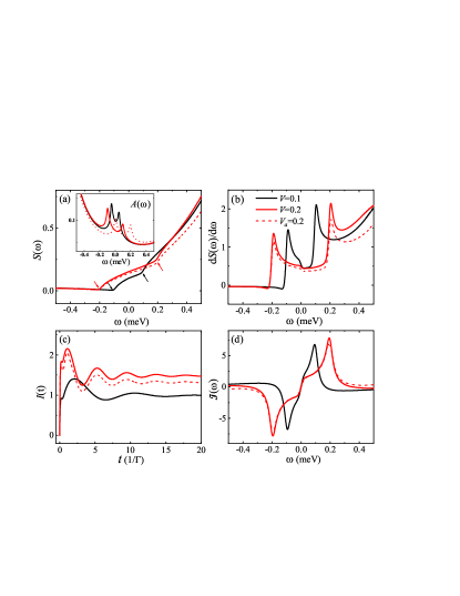
Figure 3: (Color online) The numerical results of the Kondo characteristics on (a) circuit noise spectrum $S(\omega)$ (in $10^{-8}$ eA); (b) ${\rm d}S(\omega)/{\rm d}\omega$ (in $10^{-5}$A/V); (c)The real-time dynamics of the transport current $I(t)$ (in pA); (d) The sine transform of transient current, ${\cal J}(\omega)=\int^{\infty}_{0}\!{\rm d}t\,\sin(\omega t)\delta I(t)$. The inset in (a) is the DOS $A(\omega)$. We adopt the values of bias voltage (in meV): $V=0.1$ (black) and $0.2$ (red). The red-dashed curve is for the asymmetrical bias voltage denoted by $V_{a}=0.2$ with $\mu_{\rm L}=0.2$meV and $\mu_{\rm R}=0$.

Figure 3(a) reports the evaluated current noise spectrum $S(\omega)$, at different values of the applied bias voltage. Comparing to its equilibrium counterpart, Fig. 1(a), the applied bias voltage splits the Kondo characteristic, from the single inflection point at $\omega=0$, into two asymmetric upturns around $\omega=\pm|\mu_{\rm L}-\mu_{\rm R}|=\pm eV$. These differ also from the nonequilibrium Kondo characteristic in the DOS $A(\omega)$, the inset of Fig. 3(a), with the peaks at individual $\mu_{\rm L}$ and $\mu_{\rm R}$ Mei932601 ; Leb01035308 . The two asymmetric upturns in $S(\omega)$ turn into two remarkable peaks in ${\rm d}S(\omega)/{\rm d}\omega$, at $\omega=\pm eV$, as plotted in Fig. 3(b).

To highlight the fact that the Kondo characteristic in $S(\omega)$ is concerned only with the difference between two Fermi energies, we consider also the case of the asymmetrical bias voltage. The red-dash curves in Fig.3 report the case of $\mu_{\rm L}=0.2$ meV and $\mu_{\rm R}=0$. The Kondo chareristics appears at the same frequencies as the symmetrical bias voltage case (red-solid) with the same Fermi energies difference.

The scenario in $S(\omega)$ differs from that in $A(\omega)$. The latter is depicted in the inset of Fig. 3(a), where the Kondo resonance follows the individual $\mu_{\rm L}$ and $\mu_{\rm R}$. This is related to the formation of Kondo singlet at the Fermi surfaces Mei932601 ; Leb01035308 . While the DOS $A(\omega)$ reflects the structure information, the current noise spectrum is related to not only the structure but also the transport current dynamics. The transient current $I(t)$ reported in Fig. 3(c) displays Kondo oscillation dynamics as consistent with the previous work Che15033009 . This Kondo oscillation comes from the Rabi interference between two Kondo resonance transport channels of $\mu_{\rm L}$ and $\mu_{\rm R}$. This type of interference does not exist in the non-Kondo regime as exemplified in Fig. 2(c). Further depicting the sine transform of the transient current ${\cal J}(\omega)$ in Fig.3(d), it exhibits the dip and peak at $\omega=-eV$ and $\omega=eV$, respectively. This feature is also remarkably different from that of the non-Kondo regime as shown in Fig.2(d). The Kondo oscillation frequency of the transient current is $|eV|=|\mu_{\rm L}-\mu_{\rm R}|$ and independent of the specific Fermi energies (see the red-solid versus the red-dash). Note that the appearance of the dip/peak at $\omega=\pm eV$ comes from the nature of the sine transformation, i.e., ${\cal J}(\omega)=-{\cal J}(-\omega)$. We now conclude that the Kondo characteristic in the noise spectrum reflects the Rabi interference of the transport current dynamics. The emergence of Kondo feature located at $\omega=\pm eV$ in $S(\omega)$ contains the information of the Kondo oscillation frequency $|eV|$. Evidently, there is a bridge between the nonequilibrium Kondo noise and the transient current. By comparing to the non-Kondo regime, Fig. 2(b) and (d), emerged in the Kondo regime, Fig. 3(b) and (d) are also minor but distinguished inflections near zero-frequency. Comparing further to the equilibrium Kondo counterpart, Fig. 1, we could conclude that the observed inflection characteristic in $\omega\in[-eV,+eV]$ is a sort of Kondo–Fano interference. This engages both Kondo characteristics at $-eV$ and $+eV$, which differs from the anti-Stokes cotunneling feature at $-eV$ only, as seen in Fig. 2(a) and (b).

As the Kondo feature is concerned, $S(\omega)$ and ${\rm d}S(\omega)/{\rm d}\omega$ in the emission ($\omega<0$) region is more distinguishable than the absorption ($\omega>0$) region; see Fig. 3. The spectroscopic information in $\omega>0$ is complicated by the sequential tunneling resonances at $\omega=\Delta^{\alpha}_{\mbox{\tiny S}}$ and $\Delta^{\alpha}_{\text{\tiny D}}$ of Eq. (17). The observation here goes often in practical reporting experimental results of the Kondo noise spectrum in the $\omega<0$ region Bas12046802 ; Del18041412 . The visualization in the $\omega>0$ region would be possible when there is clear separation between the Kondo and the sequential resonances Bas10166801 .

IV Summary

In summary, we have investigated the circuit current noise spectrum through an Anderson impurity quantum dot and underlying transient dynamics in the Kondo regime. Based on the DEOM evaluations, we first demonstrate the equilibrium case, where the Kondo resonance peak in the DOS, $A(\omega)$, is rather symmetric around $\omega=0$. The responding Kondo characteristic in the noise spectrum $S(\omega)$ exhibits an inflection point, and that in ${\rm d}S(\omega)/{\rm d}\omega$, turns out to be a remarkable Fano–type resonant peak, at $\omega=0$.

It is well–known that the noise spectrum can be tuned by bias voltage. The related absorption mechanism, with the electron sequential tunneling resonances at $\Delta^{\alpha}_{\text{\tiny{S,D}}}$ of Eq. (17). On the other hand, $A(\omega)$ directly reflects the two Hubbard resonances at $E_{\text{\tiny{S,D}}}$ that are independent of the bias voltage. The tunneling resonances at $\Delta^{\alpha}_{\text{\tiny{S,D}}}$ are the non-Markovian quasi-steps and Lorentzian-like peaks, in $S(\omega)$ Jin11053704 ; Eng04136602 ; Rot09075307 and ${\rm d}S(\omega)/{\rm d}\omega$, respectively.

We then study the nonequilibrium Kondo characteristics. The applied bias voltage splits the characteristic in $S(\omega)$, from the single inflection point at $\omega=0$, into two asymmetric upturns around $\omega=\pm|\mu_{\rm L}-\mu_{\rm R}|=\pm eV$. Meanwhile, in ${\rm d}S(\omega)/{\rm d}\omega$ the Kondo features are two remarkable peaks. We demonstrate that the observed absorptive/emissive Kondo resonance is concerned only with $eV=\mu_{\rm L}-\mu_{\rm R}$. This differs from the DOS $A(\omega)$, where the Kondo resonance peaks reflect rather the structure information for the shifted Fermi energies of $\mu_{\rm L}$ and $\mu_{\rm R}$. In other words, the DOS describes the formation of Kondo resonance singlet states on individual nonequilibrium Fermi surfaces.

Current noise spectrum is related to not only the structure but also the transport current dynamics. Further demonstrations include also the transient circuit current. Evidently, the nonequilibrium Kondo features at $\omega=\pm eV$ originate from the Kondo oscillation of the transport current. Moreover, we compare the noise spectra between the non-Kondo and Kondo regimes and between the equilibrium and nonequilibrium cases. The observed overall inflection characteristics within $\omega\in[-eV,eV]$ indicate a sort of Kondo–Fano interference. This engages both Kondo characteristics at $-eV$ and $+eV$, which differs from the anti-Stokes cotunneling feature at $-eV$ only. The emission noise Kondo feature is often more distinguishable than the absorption, as the latter would be contaminated by the sequential tunneling signals. This work is closely related to the experiments Bas10166801 ; Bas12046802 ; Del18041412 . It could be anticipated that the present results can be readily demonstrated in the current experiments.

- (1) Y. M. Blanter and M. Büttiker, Phys. Rep. 336, 1 (2000).
- (2) I. Imry, Introduction to Mesoscopic Physics, Oxford university press, 2002.
- (3) C. Beenakker and C. Schnenberger, Phys. Today 56, 37 (2003).
- (4) Quantum Noise in Mesoscopic Physics, Kluwer, Dordrecht, 2003, edited by Y. V. Nazarov.
- (5) R. de Picciotto et al., Nature 389, 162 (1997).
- (6) M. Reznikov, R. d. Picciotto, T. G. Griffiths, M. Heiblum, and V. Umansky, Nature 399, 238 (1999).
- (7) A. Bid, N. Ofek, M. Heiblum, V. Umansky, and D. Mahalu, Phys. Rev. Lett. 103, 236802 (2009).
- (8) A. A. Kozhevnikov, R. J. Schoelkopf, and D. E. Prober, Phys. Rev. Lett. 84, 3398 (2000).
- (9) F. Lefloch, C. Hoffmann, M. Sanquer, and D. Quirion, Phys. Rev. Lett. 90, 067002 (2003).
- (10) O. Entin-Wohlman, Y. Imry, S. A. Gurvitz, and A. Aharony, Phys. Rev. B 75, 193308 (2007).
- (11) X. Q. Li, P. Cui, and Y. J. Yan, Phys. Rev. Lett. 94, 066803 (2005).
- (12) S. D. Barrett and T. M. Stace, Phys. Rev. Lett. 96, 017405 (2006).
- (13) J. Gabelli and B. Reulet, Phys. Rev. Lett. 100, 026601 (2008).
- (14) J. Wabnig, B. W. Lovett, J. H. Jefferson, and G. A. D. Briggs, Phys. Rev. Lett. 102, 016802 (2009).
- (15) Y. LIU, J. JIN, J. LI, X. LI, and Y. YAN, SCIENCE CHINA Physics, Mechanics & Astronomy 56, 1866 (2013).
- (16) J. S. Jin, M. Marthaler, P.-Q. Jin, D. Golubev, and G. Schön, New J. Phys. 15, 025044 (2013).
- (17) J. S. Jin, X. Q. Li, M. Luo, and Y. J. Yan, J. Appl. Phys. 109, 053704 (2011).
- (18) H.-A. Engel and D. Loss, Phys. Rev. Lett. 93, 136602 (2004).
- (19) E. A. Rothstein, O. Entin-Wohlman, and A. Aharony, Phys. Rev. B 79, 075307 (2009).
- (20) P.-Y. Yang, C.-Y. Lin, and W.-M. Zhang, Phys. Rev. B 89, 115411 (2014).
- (21) J. Basset, H. Bouchiat, and R. Deblock, Phys. Rev. Lett. 105, 166801 (2010).
- (22) J. Basset et al., Phys. Rev. Lett. 108, 046802 (2012).
- (23) R. Delagrange, J. Basset, H. Bouchiat, and R. Deblock, Phys. Rev. B 97, 041412 (2018).
- (24) C. P. Moca, P. Simon, C. H. Chung, and G. Zaránd, Phys. Rev. B 83, 201303 (2011).
- (25) S. Y. Müller, M. Pletyukhov, D. Schuricht, and S. Andergassen, Phys. Rev. B 87, 245115 (2013).
- (26) A. Crépieux, S. Sahoo, T. Q. Duong, R. Zamoum, and M. Lavagna, Phys. Rev. Lett. 120, 107702 (2018).
- (27) J. S. Jin, S. K. Wang, X. Zheng, and Y. J. Yan, J. Chem. Phys. 142, 234108 (2015).
- (28) Y. J. Yan, J. Chem. Phys. 140, 054105 (2014).
- (29) Y. J. Yan, J. S. Jin, R. X. Xu, and X. Zheng, Frontiers Phys. 11, 110306 (2016).
- (30) H. D. Zhang, R. X. Xu, X. Zheng, and Y. J. Yan, Mol. Phys. 116, 780 (2018), Special Issue, “Molecular Physics in China”.
- (31) Y. Wang, R. X. Xu, and Y. J. Yan, J. Chem. Phys. 152, 041102 (2020).
- (32) H. D. Zhang, Q. Qiao, R. X. Xu, and Y. J. Yan, Chem. Phys. 481, 237 (2016).
- (33) H. D. Zhang, Q. Qiao, R. X. Xu, and Y. J. Yan, J. Chem. Phys. 145, 204109 (2016).
- (34) Y. X. Cheng et al., Sci. China-Phys. Mech. Astron. 63, 297811 (2020).
- (35) Y. D. Wang, J. H. Wei, and Y. J. Yan, J. Chem. Phys. 152, 164113 (2020).
- (36) H. Gong et al., J. Chem. Phys. 153, 154111 (2020).
- (37) J. S. Jin, Phys. Rev. B 101, 235144 (2020).
- (38) J. S. Jin, X. Zheng, and Y. J. Yan, J. Chem. Phys. 128, 234703 (2008).
- (39) X. Zheng et al., Prog. Chem. 24, 1129 (2012),
- (40) X. Zheng, Y. J. Yan, and M. Di Ventra, Phys. Rev. Lett. 111, 086601 (2013).
- (41) Z. H. Li et al., Phys. Rev. Lett. 109, 266403 (2012).
- (42) D. Hou et al., J. Chem. Phys. 142, 104112 (2015).
- (43) L. Z. Ye et al., WIREs Comp. Mol. Sci. 6, 608 (2016).
- (44) J. Hu, R. X. Xu, and Y. J. Yan, J. Chem. Phys. 133, 101106 (2010).
- (45) J. Hu, M. Luo, F. Jiang, R. X. Xu, and Y. J. Yan, J. Chem. Phys. 134, 244106 (2011).
- (46) H. D. Zhang, Q. Qiao, R. X. Xu, X. Zheng, and Y. J. Yan, J. Chem. Phys. 147, 044105 (2017).
- (47) L. Han, H. D. Zhang, X. Zheng, and Y. J. Yan, J. Phys. Chem. 148, 234108 (2018).
- (48) A. W. Holleitner, C. R. Decker, H. Qin, K. Eberl, and R. H. Blick, Phys. Rev. Lett. 87, 256802 (2001).
- (49) Y. Meir, N. S. Wingreen, and P. A. Lee, Phys. Rev. Lett. 70, 2601 (1993).
- (50) H. Haug and A.-P. Jauho, Quantum Kinetics in Transport and Optics of Semiconductors, Springer-Verlag, Berlin, 2nd, substantially revised edition, 2008, Springer Series in Solid-State Sciences 123.
- (51) E. Lebanon and A. Schiller, Phys. Rev. B 65, 035308 (2001).
- (52) Y. X. Cheng et al., New J. Phys. 17, 033009 (2015).