Exploiting Chain Rule and Bayes’ Theorem to
Compare Probability Distributions

Abstract

To measure the difference between two probability distributions, referred to as the source and target, respectively, we exploit both the chain rule and Bayes’ theorem to construct conditional transport (CT), which is constituted by both a forward component and a backward one. The forward CT is the expected cost of moving a source data point to a target one, with their joint distribution defined by the product of the source probability density function (PDF) and a source-dependent conditional distribution, which is related to the target PDF via Bayes’ theorem. The backward CT is defined by reversing the direction. The CT cost can be approximated by replacing the source and target PDFs with their discrete empirical distributions supported on mini-batches, making it amenable to implicit distributions and stochastic gradient descent-based optimization. When applied to train a generative model, CT is shown to strike a good balance between mode-covering and mode-seeking behaviors and strongly resist mode collapse. On a wide variety of benchmark datasets for generative modeling, substituting the default statistical distance of an existing generative adversarial network with CT is shown to consistently improve the performance. PyTorch code is provided.

1 Introduction

Measuring the difference between two probability distributions is a fundamental problem in statistics and machine learning [1, 2, 3]. A variety of statistical distances, such as the Kullback–Leibler (KL) divergence [4], Jensen–Shannon (JS) divergence [5], maximum mean discrepancy (MMD) [6], and Wasserstein distance [7], have been proposed to quantify the difference. They have been widely used for generative modeling with different mode covering/seeking behaviors [8, 9, 10, 11, 12, 13]. The KL divergence, directly related to both maximum likelihood estimation and variational inference [14, 15, 16], requires the two probability distributions to share the same support and is often inapplicable if either is an implicit distribution whose probability density function (PDF) is unknown [17, 18, 19, 20]. Variational auto-encoders (VAEs) [8], the KL divergence based deep generative models, are stable to train, but often exhibit mode-covering behaviors in its generated data, producing blurred images. The JS divergence is directly related to the min-max loss of a generative adversarial net (GAN) when the discriminator is optimal [9], while the Wasserstein-1 distance is directly related to the min-max loss of a Wasserstein GAN [11], whose critic is optimized under the 1-Lipschitz constraint. However, it is difficult to maintain a good balance between the updates of the generator and discriminator/critic, making (Wasserstein) GANs notoriously brittle to train. MMD [6] is an RKHS-based statistical distance behind MMD-GANs [21, 22, 10], which have also shown promising results in generative modeling when trained with a min-max loss. Different from VAEs, these GAN-based models often exhibit mode dropping and face the danger of mode collapse if not well tuned during the training.

In this paper, we introduce conditional transport (CT) as a new method to quantify the difference between two probability distributions, which will be referred to as the source distribution $p_{X}(\boldsymbol{x})$ and target distribution $p_{Y}(\boldsymbol{y})$, respectively. The construction of CT is motivated by the following observation: the difference between $p_{X}(\boldsymbol{x})$ and $p_{Y}(\boldsymbol{y})$ can be reflected by the expected difference of two dependent random variables $\boldsymbol{x}$ and $\boldsymbol{y}$, whose joint distribution $\pi(\boldsymbol{x},\boldsymbol{y})$ is constrained by both $p_{X}(\boldsymbol{x})$ and $p_{Y}(\boldsymbol{y})$ in a certain way. Denoting $c(\boldsymbol{x},\boldsymbol{y})\geq 0$ as a cost function to measure the difference between points $\boldsymbol{x}$ and $\boldsymbol{y}$, such as $c(\boldsymbol{x},\boldsymbol{y})=\|\boldsymbol{x}-\boldsymbol{y}\|_{2}^{2}$, the expected difference is expressed as $\mathbb{E}_{\pi(\boldsymbol{x},\boldsymbol{y})}[c(\boldsymbol{x},\boldsymbol{y})]$. A basic way to constrain $\pi(\boldsymbol{x},\boldsymbol{y})$ with both $p_{X}(\boldsymbol{x})$ and $p_{Y}(\boldsymbol{y})$ is to let $\pi(\boldsymbol{x},\boldsymbol{y})=p_{X}(\boldsymbol{x})p_{Y}(\boldsymbol{y})$, which means drawing $\boldsymbol{x}$ and $\boldsymbol{y}$ independently from $p_{X}(\boldsymbol{x})$ and $p_{Y}(\boldsymbol{y})$, respectively; this expected difference $\mathbb{E}_{p_{X}(\boldsymbol{x})p_{Y}(\boldsymbol{y})}[c(\boldsymbol{x},\boldsymbol{y})]$ is closely related to the energy distance [23]. Another constraining method is to require both $\int\pi(\boldsymbol{x},\boldsymbol{y})d\boldsymbol{y}=p_{X}(\boldsymbol{x})$ and $\int\pi(\boldsymbol{x},\boldsymbol{y})d\boldsymbol{x}=p_{Y}(\boldsymbol{y})$, under which ${\min_{\pi}}\{\mathbb{E}_{\pi(\boldsymbol{x},\boldsymbol{y})}[c(\boldsymbol{x},\boldsymbol{y})]\}$ becomes the Wasserstein distance [7, 24, 25, 26].

A key insight of this paper is that by exploiting the chain rule and Bayes’ theorem, there exist two additional ways to constrain $\pi(\boldsymbol{x},\boldsymbol{y})$ with both $p_{X}(\boldsymbol{x})$ and $p_{Y}(\boldsymbol{y})$: 1) A forward CT that can be viewed as moving the source to target distribution; 2) A backward CT that reverses the direction. Our intuition is that given a source (target) point, it is more likely to be moved to a target (source) point closer to it. More specifically, if the target distribution does not provide good coverage of the source density, then there will exist source data points that lie in low-density regions of the target, making the expected cost of the forward CT high. Therefore, we expect that minimizing the forward CT will encourage the target distribution to exhibit a mode-covering behavior with respect to (w.r.t.) the source PDF. Reversing the direction, we expect that minimizing the backward CT will encourage the target distribution to exhibit a mode-seeking behavior w.r.t. the source PDF. Minimizing the combination of both is expected to strike a good balance between these two distinct behaviors.

To demonstrate the use of CT, we apply it to train implicit (or explicit) distributions to model both 1D and 2D toy data, MNIST digits, and natural images. The implicit distribution is defined by a deep generative model (DGM) that is simple to sample from. We provide empirical evidence to show how to control the mode-covering versus mode-seeking behaviors by adjusting the ratio of the forward CT versus backward CT. To train a DGM for natural images, we focus on adapting existing GANs, with minimal changes to their settings except for substituting the statistical distances in their loss functions with CT. We leave tailoring the network architectures and settings to CT for future study. Modifying the loss functions of various existing DGMs with CT, our experiments show consistent improvements in not only quantitative performance and generation quality, but also learning stability. Our code is available at https://github.com/JegZheng/CT-pytorch.

2 Chain rule and Bayes’ theorem based conditional transport

Exploiting the chain rule and Bayes’ theorem, we can constrain $\pi(\boldsymbol{x},\boldsymbol{y})$ with both $p_{X}(\boldsymbol{x})$ and $p_{Y}(\boldsymbol{y})$ in two different ways, leading to the forward CT and backward CT, respectively. To define the forward CT, we use the chain rule to factorize the joint distribution as

$$\pi(\boldsymbol{x},\boldsymbol{y})=p_{X}(\boldsymbol{x})\pi_{Y}(\boldsymbol{y}\,|\,\boldsymbol{x}),$$

where $\pi_{Y}(\boldsymbol{y}\,|\,\boldsymbol{x})$ is a conditional distribution of $\boldsymbol{y}$ given $\boldsymbol{x}$. This construction ensures $\int\pi(\boldsymbol{x},\boldsymbol{y})d\boldsymbol{y}=p_{X}(\boldsymbol{x})$ but not $\int\pi(\boldsymbol{x},\boldsymbol{y})d\boldsymbol{x}=p_{Y}(\boldsymbol{y})$. Denote $d_{\boldsymbol{\phi}}({\boldsymbol{h}}_{1},{\boldsymbol{h}}_{2})\in\mathbb{R}$ as a function parameterized by $\boldsymbol{\phi}$, which measures the difference between two vectors ${\boldsymbol{h}}_{1},{\boldsymbol{h}}_{2}\in\mathbb{R}^{H}$ of dimension $H$. While allowing $\int\pi(\boldsymbol{x},\boldsymbol{y})d\boldsymbol{x}\neq p_{Y}(\boldsymbol{y})$, to appropriately constraint $\pi(\boldsymbol{x},\boldsymbol{y})$ by $p_{Y}(\boldsymbol{y})$, we treat $p_{Y}(\boldsymbol{y})$ as the prior distribution, view $e^{-d_{\boldsymbol{\phi}}(\boldsymbol{x},\boldsymbol{y})}$ as an unnormalized likelihood term, and follow Bayes’ theorem to define

$$\pi_{Y}(\boldsymbol{y}\,|\,\boldsymbol{x})=e^{-d_{\boldsymbol{\phi}}(\boldsymbol{x},\boldsymbol{y})}p_{Y}(\boldsymbol{y})/Q(\boldsymbol{x}),~{}~{}\textstyle Q(\boldsymbol{x}):=\int e^{-d_{\boldsymbol{\phi}}(\boldsymbol{x},\boldsymbol{y})}p_{Y}(\boldsymbol{y})\text{d}\boldsymbol{y},$$ (1)

where $Q(\boldsymbol{x})$ is a normalization term that ensures $\int\pi_{Y}(\boldsymbol{y}\,|\,\boldsymbol{x})d\boldsymbol{y}=1$. We refer to $\pi_{Y}(\boldsymbol{y}\,|\,\boldsymbol{x})$ as the forward “navigator,” which specifies how likely a given $\boldsymbol{x}$ will be mapped to a target point $\boldsymbol{y}\sim p_{Y}(\boldsymbol{y})$. We now define the cost of the forward CT as

$$\mathcal{C}(X\rightarrow Y)=\mathbb{E}_{\boldsymbol{x}\sim p_{X}(\boldsymbol{x})}\mathbb{E}_{\boldsymbol{y}\sim\pi_{Y}(\boldsymbol{\cdot}\,|\,\boldsymbol{x})}[c(\boldsymbol{x},\boldsymbol{y})].$$ (2)

In the forward CT, we expect large $c(\boldsymbol{x},\boldsymbol{y})$ to typically co-occur with small $\pi_{Y}(\boldsymbol{y}\,|\,\boldsymbol{x})$ as long as $p_{Y}(\boldsymbol{y})$ provides a good coverage of the density of $\boldsymbol{x}$. Thus minimizing the forward CT cost is expected to encourage $p_{Y}(\boldsymbol{y})$ to exhibit a mode-covering behavior w.r.t. $p_{X}(\boldsymbol{x})$. Such kind of behavior is also expected when minimizing the forward KL divergence as $\mathrm{KL}(p_{X}||p_{Y})=\mathbb{E}_{\boldsymbol{x}\sim p_{X}}\big{[}\ln\frac{p_{X}(\boldsymbol{x})}{p_{Y}(\boldsymbol{x})}\big{]}$, which calls for $p_{Y}(\boldsymbol{x})>0$ whenever $p_{X}(\boldsymbol{x})>0$.

Reversing the direction, we construct the backward CT, where the joint is factorized as $\pi(\boldsymbol{x},\boldsymbol{y})=p_{Y}(\boldsymbol{y})\pi_{X}(\boldsymbol{x}\,|\,\boldsymbol{y})$ and the backward navigator is defined as

$$\pi_{X}(\boldsymbol{x}\,|\,\boldsymbol{y})=e^{-d_{\boldsymbol{\phi}}(\boldsymbol{x},\boldsymbol{y})}p_{X}(\boldsymbol{x})/Q(\boldsymbol{y}),~{}~{}~{}\textstyle Q(\boldsymbol{y}):=\int e^{-d_{\boldsymbol{\phi}}(\boldsymbol{x},\boldsymbol{y})}p_{X}(\boldsymbol{x})\text{d}\boldsymbol{x}.$$ (3)

This ensures $\int\pi(\boldsymbol{x},\boldsymbol{y})d\boldsymbol{x}=p_{Y}(\boldsymbol{y})$; while allowing $\int\pi(\boldsymbol{x},\boldsymbol{y})d\boldsymbol{y}\neq p_{X}(\boldsymbol{x})$, it constrains $\pi(\boldsymbol{x},\boldsymbol{y})$ by treating $p_{X}(\boldsymbol{x})$ as the prior to construct $\pi_{X}(\boldsymbol{x}\,|\,\boldsymbol{y})$. The backward CT cost is now defined as

$$\textstyle\mathcal{C}(X\leftarrow Y) =\mathbb{E}_{\boldsymbol{y}\sim p_{Y}(\boldsymbol{y})}\mathbb{E}_{\boldsymbol{x}\sim\pi_{X}(\boldsymbol{\cdot}\,|\,\boldsymbol{y})}[c(\boldsymbol{x},\boldsymbol{y})].$$ (4)

In the backward CT, we expect large $c(\boldsymbol{x},\boldsymbol{y})$ to typically co-occur with small ${\pi}_{X}(\boldsymbol{x}\,|\,\boldsymbol{y})$ as long as $p_{X}(\boldsymbol{x})$ has good coverage of the density of $\boldsymbol{y}$. Thus minimizing the backward CT cost is expected to encourage $p_{Y}(\boldsymbol{y})$ to exhibit a mode-seeking behavior w.r.t. $p_{X}(\boldsymbol{x})$. Such kind of behavior is also expected when minimizing the reverse KL divergence as $\mathrm{KL}(p_{Y}||p_{X})=\mathbb{E}_{\boldsymbol{x}\sim p_{Y}}\big{[}\ln\frac{p_{Y}(\boldsymbol{x})}{p_{X}(\boldsymbol{x})}\big{]}$, which allows $p_{Y}(\boldsymbol{x})=0$ when $p_{X}(\boldsymbol{x})>0$ and it is fine for $p_{Y}$ to just fit some portion of $p_{X}$.

In comparison to the forward and revers KLs, the proposed forward and backward CT are more broadly applicable as they don’t require $p_{X}$ and $p_{Y}$ to share the same distribution support and have analytic PDFs. For the cases where the KLs can be evaluated, we introduce

$$\mbox{D}(X,Y)=\mbox{KL}(p_{X}||p_{Y})-\mbox{KL}(p_{Y}||p_{X})$$

as a formal way to quantify the mode-seeking and mode-covering behavior of $p_{Y}$ w.r.t. $p_{X}$, with $\mbox{D}(X,Y)>0$ implying mode seeking and with $D(X,Y)<0$ implying mode covering.

Combining both the forward and backward CTs, we now define the CT cost as

$$\mathcal{C}_{\rho}(X,Y):=\textstyle\rho\mathcal{C}(X\rightarrow Y)+(1-\rho)\mathcal{C}(X\leftarrow Y),$$ (5)

where $\rho\in[0,1]$ is a parameter that can be adjusted to encourage $p_{Y}(\boldsymbol{y})$ to exhibit w.r.t. $p_{X}(\boldsymbol{x})$ mode-seeking ($\rho=0$), mode-covering ($\rho=1$), or a balance of two distinct behaviors ($\rho\in(0,1)$). By definition we have $\mathcal{C}_{\rho}(X,Y)\geq 0$, where the equality can be achieved when $p_{X}=p_{Y}$ and the navigator parameter $\boldsymbol{\phi}$ is optimized such that $e^{-d_{\boldsymbol{\phi}}(\boldsymbol{x},\boldsymbol{y})}$ is equal to one if and only if $\boldsymbol{x}=\boldsymbol{y}$ and zero otherwise. We also have $\mathcal{C}_{\rho=0.5}(X,Y)=\mathcal{C}_{\rho=0.5}(Y,X)$. We fix $\rho=0.5$ unless specified otherwise.

2.1 Conjugacy based analytic conditional distributions

Estimating the forward and backward CTs involves $\pi_{Y}(\boldsymbol{y}\,|\,\boldsymbol{x})$ and $\pi_{X}(\boldsymbol{x}\,|\,\boldsymbol{y})$, respectively. Both conditional distributions, however, are generally intractable to evaluate and sample from, unless $p_{X}(\boldsymbol{x})$ and $p_{Y}(\boldsymbol{y})$ are conjugate priors for likelihoods proportional to $e^{-d(\boldsymbol{x},\boldsymbol{y})}$, $i.e.$, $\pi_{X}(\boldsymbol{x}\,|\,\boldsymbol{y})$ and $\pi_{Y}(\boldsymbol{y}\,|\,\boldsymbol{x})$ are in the same probability distribution family as $p_{X}(\boldsymbol{x})$ and $p_{Y}(\boldsymbol{y})$, respectively. For example, if $d(\boldsymbol{x},\boldsymbol{y})=\|\boldsymbol{x}-\boldsymbol{y}\|_{2}^{2}$ and both $p_{X}(\boldsymbol{x})$ and $p_{Y}(\boldsymbol{y})$ are multivariate normal distributions, then both $\pi_{X}(\boldsymbol{x}\,|\,\boldsymbol{y})$ and $\pi_{Y}(\boldsymbol{y}\,|\,\boldsymbol{x})$ will follow multivariate normal distributions.

To be more specific, we provide a univariate normal based example, with $x,y,\phi,\theta\in\mathbb{R}$ and

$$p_{X}(x)=\mathcal{N}(0,1),~{}p_{Y}(y)=\mathcal{N}(0,e^{\theta}),~{}d_{\phi}(x,y)={(x-y)^{2}}/({2e^{\phi}}),~{}c(x,y)=(x-y)^{2}.$$ (6)

Here we have $\mbox{D}(X,Y)=\mbox{KL}[\mathcal{N}(0,1)||\mathcal{N}(0,e^{\theta})]-\mbox{KL}[\mathcal{N}(0,e^{\theta})||\mathcal{N}(0,1)]=\theta-sinh(\theta)$, which is positive when $\theta<0$, implying mode-seeking, and negative when $\theta>0$, implying mode-covering. As shown in Appendix C, we have analytic forms of the forward and backward navigators as

$$\pi_{Y}(y\,|\,x)=\mathcal{N}(\sigma(\theta-\phi)x,\sigma(\theta-\phi)e^{\phi}),~{}~{}~{}\pi_{X}(x\,|\,y)=\mathcal{N}(\sigma(-\phi)y,\sigma(\phi)),$$

where $\sigma(a)=1/(1+e^{-a})$ denotes the sigmoid function, and forward and backward CT costs as

$$\mathcal{C}(X\rightarrow Y)=\sigma(\phi-\theta)(e^{\theta}+\sigma(\phi-\theta)),~{}~{}~{}\mathcal{C}(X\leftarrow Y)=\sigma(\phi)(1+\sigma(\phi)e^{\theta}).$$

As a proof of concept, we illustrate the optimization under CT using the above example, for which $\theta=0$ is the optimal solution that makes $p_{X}=p_{Y}$. Thus when applying gradient descent to minimize the CT cost $\mathcal{C}_{\rho=0.5}(X,Y)$, we expect the generator parameter $\theta\rightarrow 0$ with proper learning dynamic, as long as the learning of the navigator parameter $\phi$ is appropriately controlled. This is confirmed by Fig. 1, which shows that as the navigator $\phi$ gets optimized by minimizing CT cost, it is more obvious that $\theta$ will minimize the CT cost at zero. This suggests that the navigator parameter $\phi$ mainly plays the role in assisting the learning of $\theta$. The right four subplots describe the log-scale curves of forward cost, backward cost and bi-directional CT costs w.r.t. $\theta$ as $\phi$ gets optimized to four different values. It is worth noting that the forward cost is minimized at $e^{\theta}>1$, which implies a mode-covering behavior, and the backward cost is minimized at $e^{\theta}\rightarrow 0$, which implies a mode-seeking behavior, while the bi-directional cost is minimized at around the optimal solution $e^{\theta}=1$; the forward CT cost exhibits a flattened curve on the right hand side of its minimum, adding to which the backward CT cost not only moves that minimum left, making it closer to $\theta=0$, but also raises the whole curve on the right hand side, making the optimum of $\theta$ become easier to reach via gradient descent.

To apply CT in a general setting where the analytical forms of the distributions are unknown, there is no conjugacy, or we only have access to random samples from the distributions, below we show we can approximate the CT cost by replacing both $p_{X}(\boldsymbol{x})$ and $p_{Y}(\boldsymbol{y})$ with their corresponding discrete empirical distributions supported on mini-batches. Minimizing this approximate CT cost, amenable to mini-batch SGD based optimization, is found to be effective in driving the target (model) distribution $p_{Y}$ towards the source (data) distribution $p_{X}$, with the ability to control the mode-seeking and mode-covering behaviors of $p_{Y}$ w.r.t. $p_{X}$.

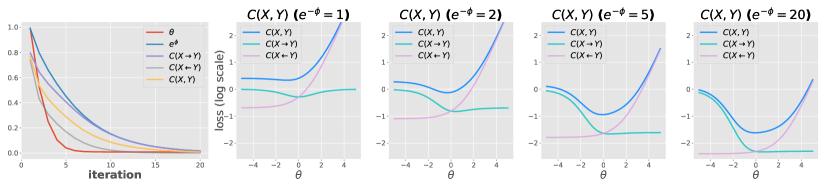
Figure 1: Illustration of minimizing the CT cost $\mathcal{C}_{\phi,\theta}(X,Y)$ between $\mathcal{N}(0,1)$ and $\mathcal{N}(0,e^{\theta})$. Left: Evolution of CT cost, its parameters, and forward and backward costs; Right: 4 CT cost curves against $\theta$ as $e^{\phi}$ is being optimized to a small value to jointly show the optimized $\phi$ provides better learning dynamic for the learning of $\theta$.

2.2 Approximate CT given empirical samples

Below we use generative modeling as an example to show how to apply the CT cost in a general setting that only requires access to random samples of both $\boldsymbol{x}$ and $\boldsymbol{y}$. Denote $\boldsymbol{x}$ as a data taking its value in $\mathbb{R}^{V}$. In practice, we observe a finite set $\mathcal{X}=\{\boldsymbol{x}_{i}\}_{i=1}^{|\mathcal{X}|}$, consisting of $|\mathcal{X}|$ data samples assumed to be $iid$ drawn from $p_{X}(\boldsymbol{x})$. Given $\mathcal{X}$, the usual task is to learn a distribution to approximate $p_{X}(\boldsymbol{x})$, for which we consider a deep generative model (DGM) defined as $\boldsymbol{y}=G_{\boldsymbol{\theta}}(\boldsymbol{\epsilon}),~{}\boldsymbol{\epsilon}\sim p(\boldsymbol{\epsilon}),$ where $G_{\boldsymbol{\theta}}$ is a generator that transforms noise $\boldsymbol{\epsilon}\sim p(\boldsymbol{\epsilon})$ via a deep neural network parameterized by $\boldsymbol{\theta}$ to generate random sample $\boldsymbol{y}\in\mathbb{R}^{V}$. While the PDF of the generator, denoted as $p_{Y}(\boldsymbol{y};\boldsymbol{\theta})$, is often intractable to evaluate, it is straightforward to draw $\boldsymbol{y}\sim p_{Y}(\boldsymbol{y};\boldsymbol{\theta})$ with $G_{\boldsymbol{\theta}}$.

While knowing neither $p_{X}(\boldsymbol{x})$ nor $p_{Y}(\boldsymbol{y};\boldsymbol{\theta})$, we can obtain discrete empirical distributions $p_{\hat{X}_{N}}$ and $p_{\hat{Y}_{M}}$ supported on mini-batches $\boldsymbol{x}_{1:N}$ and $\boldsymbol{y}_{1:M}$, as defined below, to guide the optimization of $G_{\boldsymbol{\theta}}$ in an iterative manner. With $N$ random observations sampled without replacement from $\mathcal{X}$, we define

$$\textstyle p_{\hat{X}_{N}}(\boldsymbol{x})=\frac{1}{N}\sum_{i=1}^{N}\delta{(\boldsymbol{x}-\boldsymbol{x}_{i})},~{}~{}\{\boldsymbol{x}_{1},\ldots,\boldsymbol{x}_{N}\}\subseteq\mathcal{X}$$ (7)

as an empirical distribution for $\boldsymbol{x}$. Similarly, with $M$ random samples of the generator, we define

$$\textstyle p_{\hat{Y}_{M}}(\boldsymbol{y})=\frac{1}{M}\sum_{j=1}^{M}\delta{(\boldsymbol{y}-\boldsymbol{y}_{j})},~{}\boldsymbol{y}_{j}=G_{\boldsymbol{\theta}}(\boldsymbol{\epsilon}_{j}),~{}\boldsymbol{\epsilon}_{j}\,{\scriptstyle\stackrel{{\scriptstyle iid}}{{\sim}}}\,p(\boldsymbol{\epsilon})~{}~{}.$$ (8)

Substituting $p_{Y}(\boldsymbol{y};\boldsymbol{\theta})$ in (2) with $p_{\hat{Y}_{M}}(\boldsymbol{y})$, the continuous forward navigator becomes a discrete one as

$$\textstyle\hat{\pi}_{Y}(\boldsymbol{y}\,|\,\boldsymbol{x}) =\textstyle\sum_{j=1}^{M}\hat{\pi}_{M}(\boldsymbol{y}_{j}\,|\,\boldsymbol{x},\boldsymbol{\phi})\delta_{\boldsymbol{y}_{j}},~{}~{}\hat{\pi}_{M}(\boldsymbol{y}_{j}\,|\,\boldsymbol{x},\boldsymbol{\phi}):=\textstyle\frac{e^{-d_{\boldsymbol{\phi}}(\boldsymbol{x},\boldsymbol{y}_{j})}}{\sum_{j^{\prime}=1}^{M}e^{-d_{\boldsymbol{\phi}}(\boldsymbol{x},\boldsymbol{y}_{j^{\prime}})}}.$$ (9)

Thus given $p_{\hat{Y}_{M}}$, the cost of a forward CT can be approximated as

$$\mathcal{C}_{\boldsymbol{\phi},\boldsymbol{\theta}}(X\rightarrow\hat{Y}_{M}) =\mathbb{E}_{\boldsymbol{y}_{1:M}\,{\scriptstyle\stackrel{{\scriptstyle iid}}{{\sim}}}\,p_{Y}(\boldsymbol{y};\boldsymbol{\theta})}\mathbb{E}_{\boldsymbol{x}\sim p_{X}(\boldsymbol{x})}\left[\textstyle\textstyle\sum_{j=1}^{M}c(\boldsymbol{x},\boldsymbol{y}_{j})\hat{\pi}_{M}(\boldsymbol{y}_{j}\,|\,\boldsymbol{x},\boldsymbol{\phi})\right],$$ (10)

which can be interpreted as the expected cost of following the forward navigator to stochastically transport a random source point $\boldsymbol{x}$ to one of the $M$ randomly instantiated “anchors” of the target distribution. Similar to previous analysis, we expect this approximate forward CT to stay small as long as $p_{Y}(\boldsymbol{y};\boldsymbol{\theta})$ exhibits a mode covering behavior w.r.t. $p_{X}(\boldsymbol{x})$.

Similarly, we can approximate the backward navigator and CT cost as

$$\hat{\pi}_{X}(\boldsymbol{x}\,|\,\boldsymbol{y})=\textstyle\sum_{i=1}^{N}\hat{\pi}_{N}(\boldsymbol{x}_{i}\,|\,\boldsymbol{y},\boldsymbol{\phi})\delta_{\boldsymbol{x}_{i}},~{}~{}\hat{\pi}_{N}(\boldsymbol{x}_{i}\,|\,\boldsymbol{y},\boldsymbol{\phi}):=\textstyle\frac{e^{-d_{\boldsymbol{\phi}}(\boldsymbol{x}_{i},\boldsymbol{y})}}{\sum_{i^{\prime}=1}^{N}e^{-d_{\boldsymbol{\phi}}(\boldsymbol{x}_{i^{\prime}},\boldsymbol{y})}},$$

$$\mathcal{C}_{\boldsymbol{\phi},\boldsymbol{\theta}}(\hat{X}_{N}\leftarrow Y)=\mathbb{E}_{\boldsymbol{x}_{1:M}\,{\scriptstyle\stackrel{{\scriptstyle iid}}{{\sim}}}\,p_{X}(\boldsymbol{x})}\mathbb{E}_{\boldsymbol{y}\sim p_{Y}(\boldsymbol{y};\boldsymbol{\theta})}\left[\textstyle\sum_{i=1}^{N}c(\boldsymbol{x}_{i},\boldsymbol{y})\hat{\pi}_{N}(\boldsymbol{x}_{i}\,|\,\boldsymbol{y},\boldsymbol{\phi})\right].$$ (11)

Similar to previous analysis, we expect this approximate backward CT to stay small as long as $p_{Y}(\boldsymbol{y};\boldsymbol{\theta})$ exhibits a mode-seeking behavior w.r.t. $p_{X}(\boldsymbol{x})$.

Combining (10) and (11), we define the approximate CT cost as

$$\mathcal{C}_{\boldsymbol{\phi},\boldsymbol{\theta},\rho}(\hat{X}_{N},\hat{Y}_{M})=\rho\mathcal{C}_{\boldsymbol{\phi},\boldsymbol{\theta}}(X\rightarrow\hat{Y}_{M})+(1-\rho)\mathcal{C}_{\boldsymbol{\phi},\boldsymbol{\theta}}(\hat{X}_{N}\leftarrow Y),$$ (12)

an unbiased sample estimate of which, given mini-batches $\boldsymbol{x}_{1:N}$ and $\boldsymbol{y}_{1:M}$, can be expressed as

$$\mathcal{L}_{\boldsymbol{\phi},\boldsymbol{\theta},\rho}(\boldsymbol{x}_{1:N},\boldsymbol{y}_{1:M}) =\textstyle\sum_{i=1}^{N}\sum_{j=1}^{M}c(\boldsymbol{x}_{i},\boldsymbol{y}_{j})\left(\textstyle\frac{\rho}{N}\hat{\pi}_{M}(\boldsymbol{y}_{j}\,|\,\boldsymbol{x}_{i},\boldsymbol{\phi})+\textstyle\frac{1-\rho}{M}\hat{\pi}_{N}(\boldsymbol{x}_{i}\,|\,\boldsymbol{y}_{j},\boldsymbol{\phi})\right)$$

$$\!\!\!\!\!\!\!\!\!\!\!\!\!=\textstyle\sum_{i=1}^{N}\sum_{j=1}^{M}c(\boldsymbol{x}_{i},\boldsymbol{y}_{j})\left(\textstyle\frac{\rho}{N}\textstyle\frac{e^{-d_{\boldsymbol{\phi}}(\boldsymbol{x}_{i},\boldsymbol{y}_{j})}}{\sum_{j^{\prime}=1}^{M}e^{-d_{\boldsymbol{\phi}}(\boldsymbol{x}_{i},\boldsymbol{y}_{j^{\prime}})}}+\textstyle\frac{1-\rho}{M}\textstyle\frac{e^{-d_{\boldsymbol{\phi}}(\boldsymbol{x}_{i},\boldsymbol{y}_{j})}}{\sum_{i^{\prime}=1}^{N}e^{-d_{\boldsymbol{\phi}}(\boldsymbol{x}_{i^{\prime}},\boldsymbol{y}_{j})}}\right).$$ (13)

Lemma 1.

Approximate CT in (12) is asymptotic as $\lim_{N,M\rightarrow\infty}\mathcal{C}_{\boldsymbol{\phi},\boldsymbol{\theta},\rho}(\hat{X}_{N},\hat{Y}_{M})=\mathcal{C}_{\boldsymbol{\phi},\boldsymbol{\theta},\rho}(X,Y).$

2.3 Cooperatively-trained or adversarially-trained feature encoder

To apply CT for generative modeling of high-dimensional data, such as natural images, we need to define an appropriate cost function $c(\boldsymbol{x},\boldsymbol{y})$ to measure the difference between two random points. A naive choice is some distance between their raw feature vectors, such as $c(\boldsymbol{x},\boldsymbol{y})=\|\boldsymbol{x}-\boldsymbol{y}\|_{2}^{2}$, which, however, is known to often poorly reflect the difference between high-dimensional data residing on low-dimensional manifolds. For this reason, with cosine similarity [27] as ${\textstyle\cos({\boldsymbol{h}}_{1},{\boldsymbol{h}}_{2}):=\frac{{\boldsymbol{h}}_{1}^{T}{\boldsymbol{h}}_{2}}{{\sqrt{{\boldsymbol{h}}_{1}^{T}{\boldsymbol{h}}_{1}}}{\sqrt{{\boldsymbol{h}}_{2}^{T}{\boldsymbol{h}}_{2}}}}}$, we further introduce a feature encoder $\mathcal{T}_{\boldsymbol{\eta}}(\boldsymbol{\cdot})$, parameterized by $\boldsymbol{\eta}$, to help redefine the point-to-point cost and both navigators as

$$\textstyle c_{\boldsymbol{\eta}}(\boldsymbol{x},\boldsymbol{y})=1-\cos(\mathcal{T}_{\boldsymbol{\eta}}(\boldsymbol{x}),\mathcal{T}_{\boldsymbol{\eta}}(\boldsymbol{y})),~{}~{}~{}d_{\boldsymbol{\phi}}\left(\frac{\mathcal{T}_{\boldsymbol{\eta}}(\boldsymbol{x})}{\|\mathcal{T}_{\boldsymbol{\eta}}(\boldsymbol{x})\|},\frac{\mathcal{T}_{\boldsymbol{\eta}}(\boldsymbol{y})}{\|\mathcal{T}_{\boldsymbol{\eta}}(\boldsymbol{y})\|}\right).$$ (14)

To apply the CT cost to train a DGM, we find that the feature encoder $\mathcal{T}_{\boldsymbol{\eta}}(\boldsymbol{\cdot})$ can be learned in two different ways: 1) Cooperatively-trained: Training them cooperatively by alternating between two different losses: training the generator under a fixed $\mathcal{T}_{\boldsymbol{\eta}}(\boldsymbol{\cdot})$ with the CT loss, and training $\mathcal{T}_{\boldsymbol{\eta}}(\boldsymbol{\cdot})$ under a fixed generator with a different loss, such as the GAN discriminator loss, WGAN critic loss, and MMD-GAN [10] critic loss. 2) Adversarially-trained: Viewing the feature encoder as a critic and training it to maximize the CT cost, by not only inflating the point-to-point cost, but also distorting the feature space used to construct the forward and backward navigators’ conditional distributions.

To be more specific, below we present the details for the adversarial way to train $\mathcal{T}_{\boldsymbol{\eta}}$. Given training data $\mathcal{X}$, to train the generator $G_{\boldsymbol{\theta}}$, forward navigator $\pi_{\boldsymbol{\phi}}(\boldsymbol{y}\,|\,\boldsymbol{x})$, backward navigator $\pi_{\boldsymbol{\phi}}(\boldsymbol{x}\,|\,\boldsymbol{y})$, and encoder $\mathcal{T}_{\boldsymbol{\eta}}$, we view the encoder as a critic and propose to solve a min-max problem as

$$\!\!\!\min_{\boldsymbol{\phi},\boldsymbol{\theta}}\max_{\boldsymbol{\eta}}\mathbb{E}_{\boldsymbol{x}_{1:N}\subseteq\mathcal{X},~{}\boldsymbol{\epsilon}_{1:M}\,{\scriptstyle\stackrel{{\scriptstyle iid}}{{\sim}}}\,p(\boldsymbol{\epsilon})}[\mathcal{L}_{\boldsymbol{\phi},\boldsymbol{\theta},\rho,\boldsymbol{\eta}}(\boldsymbol{x}_{1:N},\{G_{\boldsymbol{\theta}}(\boldsymbol{\epsilon}_{j})\}_{j=1}^{M})],$$ (15)

where $\mathcal{L}_{\boldsymbol{\phi},\boldsymbol{\theta},\rho,\boldsymbol{\eta}}$ is defined the same as in (13), except that we replace $c(\boldsymbol{x}_{i},\boldsymbol{y}_{j})$ and $d_{\boldsymbol{\phi}}(\boldsymbol{\cdot},\boldsymbol{\cdot})$ with their corresponding ones shown in (14) and use reparameterization in (8) to draw $\boldsymbol{y}_{1:M}:=\{G_{\boldsymbol{\theta}}(\boldsymbol{\epsilon}_{j})\}_{j=1}^{M}$. With SGD, we update $\boldsymbol{\phi}$ and $\boldsymbol{\theta}$ using $\nabla_{\boldsymbol{\phi},\boldsymbol{\theta}}\mathcal{L}_{\boldsymbol{\phi},\boldsymbol{\theta},\rho,\boldsymbol{\eta}}(\boldsymbol{x}_{1:N},\{G_{\boldsymbol{\theta}}(\boldsymbol{\epsilon}_{j})\}_{j=1}^{M}))$ and, if the feature encoder is adversarially-trained, update $\boldsymbol{\eta}$ using $-\nabla_{\boldsymbol{\eta}}\mathcal{L}_{\boldsymbol{\phi},\boldsymbol{\theta},\rho,\boldsymbol{\eta}}(\boldsymbol{x}_{1:N},\{G_{\boldsymbol{\theta}}(\boldsymbol{\epsilon}_{j})\}_{j=1}^{M}))$.

We find by experiments that both ways to learn the encoder work well, with the adversarial one generally providing better performance. It is worth noting that in (Wasserstein) GANs, while the adversarially-trained discriminator/critic plays a similar role as a feature encoder, the learning dynamics between the discriminator/critic and generator need to be carefully tuned to maintain training stability and prevent trivial solutions ($e.g.$, mode collapse). By contrast, the feature encoder of the CT cost based DGM can be stably trained in two different ways. Its update does not need to be well synchronized with the generator and can be stopped at any time of the training.

3 Related work

In practice, variational auto-encoders [8], the KL divergence based deep generative models, are stable to train, but often exhibit mode-covering behaviors and generate blurred images [28, 29, 30, 31, 32]. By contrast, both GANs and Wasserstein GANs can generate photo-realistic images, but they often suffer from stability and mode collapse issues, requiring the update of the discriminator/critic to be well synchronized with that of the generator. This paper introduces conditional transport (CT) as a new method to quantify the difference between two probability distributions. Deep generative models trained under CT not only allow the balance between mode-covering and mode-seeking behaviors to be adjusted, but also allow the encoder to be pretrained or frozen at any time during cooperative/adversarial training.

As the JS divergence requires the two distributions to have the same support, the Wasserstein distance is often considered as more appealing for generative modeling as it allows the two distributions to have non-overlapping support [24, 25, 26]. However, while GANs and Wasserstein GANs in theory are connected to the JS divergence and Wasserstein distance, respectively, several recent works show that they should not be naively understood as the minimizers of their corresponding statistical distances, and the role played by their min-max training dynamics should not be overlooked [33, 34, 35]. In particular, Fedus et al. [34] show that even when the gradient of the JS divergence does not exist and hence GANs are predicted to fail from the perspective of divergence minimization, the discriminator is able to provide useful learning signal. Stanczuk et al. [35] show that the dual form based Wasserstein GAN loss does not provide a meaningful approximation of the Wasserstein distance; while primal form based methods could better approximate the true Wasserstein distance, they in general clearly underperform Wasserstein GANs in terms of the generation quality for high-dimensional data, such as natural images, and require an inner loop to compute the transport plan for each mini-batch, leading to high computational cost [12, 36, 37, 38, 35]. See previous works for discussions on the approximation error and gradient bias when estimating the Wasserstein distance with mini-batches [39, 23, 10, 40].

MMD-GAN [21, 22, 10] that calculates the MMD statistics in the latent space of a feature encoder is the most similar to the CT cost in terms of the actual loss function used for optimization. In particular, both the MMD-GAN loss and CT loss, given mini-batches $\boldsymbol{x}_{1:N}$ and $\boldsymbol{y}_{1:M}$, involve computing the differences of all $NM$ pairs $(\boldsymbol{x}_{i},\boldsymbol{y}_{j})$. Different from MMD-GAN, there is no need in CT to choose a kernel and tune its parameters. We provide below an ablation study to evaluate both 1) MMD generator + CT encoder and 2) MMD encoder + CT generator, which shows 1) performs on par with MMD, while 2) performs clearly better than MMD and on par with CT.

4 Experimental results

Forward and backward analysis: To empirically verify our previous analysis of the mode covering (seeking) behavior of the forward (backward) CT, we train a DGM with (12) and show the corresponding interpolation weight from the forward CT cost to the backward one, which means CT_ρ reduces from forward CT ($\rho=1$), to the CT in (12) ($\rho\in(0,1)$), and to backward CT ($\rho=0$). We consider the squared Euclidean ($i.e.$ $\mathcal{L}_{2}^{2}$) distance to define both cost $c(\boldsymbol{x},\boldsymbol{y})=\|\boldsymbol{x}-\boldsymbol{y}\|_{2}^{2}$ and $d_{\boldsymbol{\phi}}(\boldsymbol{x},\boldsymbol{y})=\|\mathcal{T}_{\boldsymbol{\phi}}(\boldsymbol{x})-\mathcal{T}_{\boldsymbol{\phi}}(\boldsymbol{y})\|_{2}^{2}$, where $\mathcal{T}_{\boldsymbol{\phi}}$ denotes a neural network parameterized by $\boldsymbol{\phi}$. We consider a 1D example of a bimodal Gaussian mixture $p_{X}(x)=\frac{1}{4}\mathcal{N}(x;-5,1)+\frac{3}{4}\mathcal{N}(x;2,1)$ and a 2D example of 8-modal Gaussian mixture with equal component weight as in Gulrajani et al. [41]. We use an empirical sample set $\mathcal{X}$, consisting of $|\mathcal{X}|=5,000$ samples from both 1D and 2D cases, and illustrate in Fig. 2 the KDE of 5000 generated samples $y_{j}=G_{\boldsymbol{\theta}}(\boldsymbol{\epsilon}_{j})$ after 5000 training epochs. For the 1D case, we take 200 grids in $[-10,10]$ to approximate the empirical distribution of $\hat{p}_{X}$ and $\hat{p}_{Y}$, and report the corresponding forward KL (KL[$\hat{p}_{X}||\hat{p}_{Y}$]), reverse KL (KL[$\hat{p}_{Y}||\hat{p}_{X}$]), and their difference $\mathrm{D}(X,Y)=\text{KL}[\hat{p}_{X}||\hat{p}_{Y}]-\text{KL}[\hat{p}_{X}||\hat{p}_{Y}]$ below each corresponding sub-figure in Fig. 2.

Comparing the results of different $\rho$ in Fig. 2, it suggests that minimizing the forward CT cost only encourages the generator to exhibit mode-covering behaviors, while minimizing the backward CT cost only encourages mode-seeking behaviors. Combining both costs provides a user-controllable balance between mode covering and seeking, leading to satisfactory fitting performance, as shown in Columns 2-4. Note that for a fair comparison, we stop the fitting at the same iteration; in practice, we find if training with more iterations, both $\rho=0.75$ and $\rho=0.25$ can achieve comparable results as $\rho=0.5$ in this example. Allowing the mode covering and seeking behaviors to be controlled by adjusting $\rho$ is an attractive property of CT_ρ.

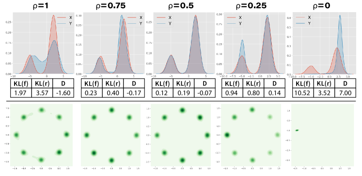
Figure 2: Forward and backward analysis: (top) Fitting 1D bi-modal Gaussian. Quantitative results of estimated forward KL (KL[$\hat{p}_{X}||\hat{p}_{Y}$]), reverse KL (KL[$\hat{p}_{Y}||\hat{p}_{X}$]), and the difference between the forward and reverse KL (D=KL[$\hat{p}_{X}||\hat{p}_{Y}$]-KL[$\hat{p}_{Y}||\hat{p}_{X}$]) are shown below each sub-figure. (bottom) 2D 8-Gaussian mixture by interpolating between the forward CT ($\rho=1$) and backward CT ($\rho=0$).

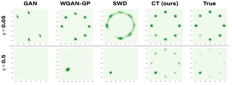
Figure 3: Experiments on the resistance to model collapse: Comparison of the generation quality on 8-Gaussian mixture data: one of the 8 modes has weight $\gamma$ and the rest modes have equal weight as $\frac{1-\gamma}{7}$.

Resistance to mode collapse: We continue to use a 8-Gaussian mixture to empirically evaluate how well a DGM resists mode collapse. Unlike the data in Fig. 2, where 8 modes are equally weighted, here the mode at the left lower corner is set to have weight $\gamma$, while the other modes are set to have the same weight of $\frac{1-\gamma}{7}$. We set $\mathcal{X}$ with 5000 samples and the mini-batch size as $N=100$. When $\gamma$ is lowered to 0.05, its corresponding mode is shown to be missed by GAN, WGAN, and SWD-based DGM, while well kept by the CT-based DGM. As an explanation, GANs are known to be susceptible to mode collapse; WGAN and SWD-based DGMs are sensitive to the mini-batch size, as when $\gamma$ equals to a small value, the samples from this mode will appear in the mini-batches less frequently than those from any other mode, amplifying their missing mode problem. Similarly, when $\gamma$ is increased to 0.5, the other modes are likely to be missed by the baseline DGMs, while the CT-based DGM does not miss any modes. The resistance of CT to mode dropping can be attributed to its forward component’s mode-covering property. The backward’s mode-seeking property further helps distinguish the density of each mode component to avoid making components of equal weight.

CT for 2D toy data and robustness in adversarial feature extraction: To test CT with more general cases, we further conduct experiments on 4 representative 2D datasets for generative modeling evaluation [41]: 8-Gaussian mixture, Swiss Roll, Half Moons, and 25-Gaussian mixture. We apply the vanilla GAN [9] and Wasserstein GAN with gradient penalty (WGAN-GP) [41] as two representatives of min-max DGMs that require solving a min-max loss. We then apply the generators trained under the sliced Wasserstein distance (SWD) [42] and CT cost as two representatives of min-max-free DGMs. Moreover, we include CT with an adversarial feature encoder trained with (14) to test the robustness of adversary and compare with the baselines in solving the min-max loss.

On each 2D data, we train these DGMs as one would normally do during the first $5k$ epochs. We then only train the generator and freeze all the other learnable model parameters, which means we freeze the discriminator in GAN, critic in WGAN, the navigator parameter $\boldsymbol{\phi}$ of the CT cost, and both $(\boldsymbol{\phi},\boldsymbol{\eta})$ of CT with an adversarial feature encoder, for another $5k$ epochs. Figs. 7-10 in Appendix E.1 illustrate this training process on each dataset, where for both min-max baseline DGMs, the models collapse after the first $5k$ epochs, while the training for SWD remains stable and that for CT continues to improve. Compared to SWD, our method covers all data density modes and moves the generator much closer to the true data density. Notably, for CT with an adversarially trained feature encoder, although it has switched from solving a min-max loss to freezing the feature encoder after 5$k$ epochs, the frozen feature encoder continues to guide the DGM to finish the training in the last $5k$ epochs, which shows the robustness of the CT cost.

(a) Adv CT.

(b) GAN.

(c) $\mathcal{L}_{D}$ + CT.

(d) SWD.

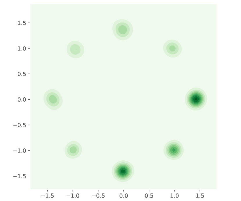
(e) Slicing + CT.

Figure 4: Ablation of fitting results by minimizing CT in different spaces: (a) CT calculated with adversarially trained encoder. (b-c) GAN vs. CT with feature space cooperatively trained with discriminator loss. (d-f) Sliced Wasserstein distance and CT in the sliced space.

   

Table 1: FID comparison with different cooperative training on CIFAR-10 (lower FID is preferred).

Critic space	FID $\downarrow$
Discriminator	29.7
Slicing	32.4
Adversarial CT	22.1

Table 2: FID Comparison with using MMD (Rational quadratic kernel/distance kernel) and CT loss in training critic/generator on CIFAR-10 (lower FID is preferred).

MMD-rq		Generator loss		MMD-dist		Generator loss
		MMD	CT			MMD	CT
Critic	MMD	39.9	24.1	Critic	MMD	40.3	28.8
loss	CT	41.4	23.9	loss	CT	30.9	29.4

Ablation of cooperatively-trained and adversarially-trained CT: As previous experiments show the adversarially-trained feature encoder could provide a valid feature space for CT cost, we further study the performance of the encoders cooperatively trained with other losses. Here we leverage, as two alternatives, the space of an encoder trained with the discriminator loss in GANs and the empirical Wasserstein distance in sliced 1D spaces [43]. We test these settings on both 8-Gaussian, as shown Fig. 4(a), and CIFAR-10 data, as shown in Table 2. It is confirmed these encoders are able to cooperatively work with CT, in general producing less appealing results with those trained by maximizing CT. From this view, although CT is able to provide guidance for the generators in the feature space learned with various options, maximizing CT is still preferred to ensure the efficiency. Moreover, as observed in Figs. 4(b)-4(e), CT clearly improves the fitting with sliced Wasserstein distance. To explain why CT helps improve in the sliced space, we further provide a toy example in 1D to study the properties of CT and empirical Wasserstein distance in Appendix E.3.

Ablation of MMD and CT: As MMD also compares the pair-wise sample relations in a mini-batch, we study if MMD and CT can benefit each other. The feature space of MMD-GAN can be considered as $\mathcal{T}_{\boldsymbol{\eta}}\circ k$, where $k$ is the rational quadratic or distance kernel in Bińkowski et al. [10]. Here we evaluate the combinations of MMD/CT as the generator/encoder criterion to train DGMs. On CIFAR-10, shown in Table 2, combining MMD and CT generally has improvement over MMD alone in FID. It is interesting to notice that for MMD-GAN, learning its generator with the CT cost shows more obvious improvement than learning its feature encoder with the CT cost. We speculate the estimation of MMD relies on a supremum of its witness function, which needs to be maximized w.r.t $\mathcal{T}_{\boldsymbol{\eta}}\circ k$ and cannot be guaranteed by maximizing CT w.r.t $\mathcal{T}_{\boldsymbol{\eta}}$. In the case of MMD-dist, using CT for witness function updates shows a more clear improvement, probably because CT has a similar form as MMD when using the distance kernel. From this view, CT and MMD are naturally able to be combined to compare the distributional difference with pair-wise sample relations. Different from MMD, CT does not involve the choice of kernel and its navigators assist to improve the comparison efficiency. Below we show on more image datasets, CT is compatible with many existing models, and achieve good results to show improvements on a variety of data with different scale.

Adversarially-trained CT for natural images: We conduct a variety of experiments on natural images to evaluate the performance and reveal the properties of DGMs optimized under the CT cost. We consider three widely-used image datasets, including CIFAR-10 [44], CelebA [45], and LSUN-bedroom [46] for general evaluation, as well as CelebA-HQ [47], FFHQ [48] for evaluation in high-resolution. We compare the results of DGMs optimized with the CT cost against DGMs trained with their original criterion including DCGAN [49], Sliced Wasserstein Generative model (SWG) [42], MMD-GAN [10], SNGAN [50], and StyleGAN2 [51]. For fair comparison, we leverage the best configurations reported in their corresponding paper or Github page. The detailed setups can be found in Appendix D. For evaluation metric, we consider the commonly used Fréchet inception distance (FID, lower is preferred) [52] on all datasets and Inception Score (IS, higher is preferred) [53] on CIFAR-10. Both FID and IS are calculated using a pre-trained inception model [54].

Table 3: Results of CT with different deep generative models on CIFAR-10, CelebA and LSUN. Base model results are quoted from corresponding paper or github page.

Method	Fréchet Inception Distance (FID $\downarrow$)			Inception Score ($\uparrow$)
	CIFAR-10	CelebA	LSUN-bedroom	CIFAR-10
DCGAN [49]	30.2$\pm$0.9	52.5$\pm$2.2	61.7$\pm$2.9	6.2$\pm$0.1
CT-DCGAN	22.1$\pm$1.1	29.4$\pm$2.0	32.6$\pm$2.5	7.5$\pm$0.1
SWG [42]	33.7$\pm$1.5	21.9$\pm$2.0	67.9$\pm$2.7	-
CT-SWG	25.9$\pm$ 0.9	18.8 $\pm$ 1.2	39.0 $\pm$ 2.1	6.9 $\pm$ 0.1
MMD-GAN [10]	39.9$\pm$0.3	20.6$\pm$0.3	32.0$\pm$0.3	6.5$\pm$0.1
CT-MMD-GAN	23.9 $\pm$ 0.4	13.8 $\pm$ 0.4	38.3 $\pm$ 0.3	7.4 $\pm$ 0.1
SNGAN [50]	21.5$\pm$1.3	21.7$\pm$1.5	31.1$\pm$2.1	8.2$\pm$0.1
CT-SNGAN	17.2$\pm$1.0	9.2$\pm$1.0	16.8$\pm$2.1	8.8$\pm$0.1
StyleGAN2 [51]	5.8	5.2	2.9	10.0
CT-StyleGAN2	2.9 $\pm$ 0.5	4.0 $\pm$ 0.7	6.3 $\pm$ 0.2	10.1 $\pm$ 0.1

The summary of FID and IS on previously mentioned model is reported in Table 3. We observe that trained with CT cost, all the models have improvements with different margin in most cases, suggesting that CT is compatible with standard GANs, SWG, MMD-GANs, WGANs and generally helps improve generation quality, especially for data with richer modalities like CIFAR-10. CT is also compatible with advanced model architecture like StyleGAN2, confirming that a better feature space could make CT more efficient to guide the generator and produce better results.

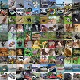
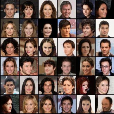
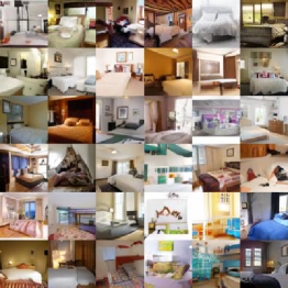
Figure 5: Generated samples of the deep generative model that adopts the backbone of SNGAN but is optimized with the CT cost on CIFAR-10, CelebA, and LSUN-Bedroom. See Appendix E for more results.

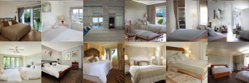
(a) LSUN-Bedroom(128x128)

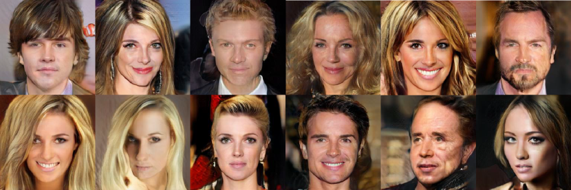
(b) CelebA-HQ(256x256)

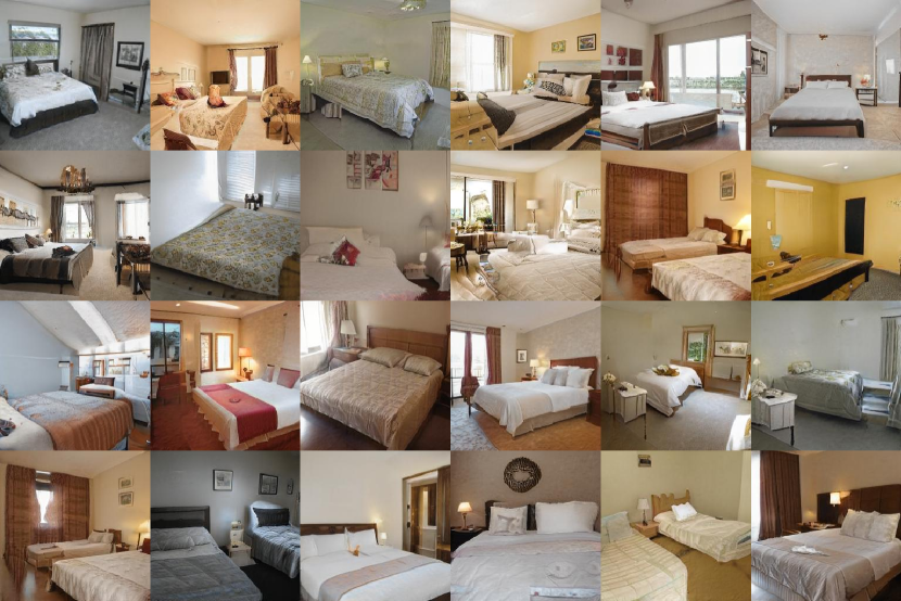
(c) LSUN-Bedroom(256x256)

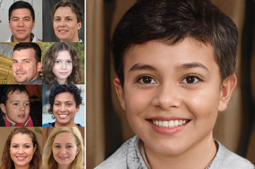
(d) FFHQ (256x256/1024x1024)

Figure 6: Generation results in higher-resolution cases, with SNGAN and StyleGAN2 architecture. Top:LSUN-Bedroom (128x128) and CelebA-HQ (256x256), done with CT-SNGAN. Bottom: LSUN-Bedroom (256x256) and FFHQ (256x256/1024x1024), done with CT-StyleGAN2.

The qualitative results shown in Fig. 5 are consistent with quantitative results in Table 3. To additionally show how CT works for more complex generation tasks, we show in Fig. 6 example higher-resolution images generated by CT-SNGAN on LSUN bedroom (128x128) and CelebA-HQ (256x256), as well as images generated by CT-StyleGAN2 on LSUN bedroom (256x256), FFHQ (256x256), and FFHQ (1024x1024).

Table 4: FID of generation results on CIFAR-10, trained with different $\rho$.

$\rho$	1	0.75	0.5	0.25	0
CT-DCGAN	25.1	22.1	22.1	21.4	72.1
CT-SNGAN	23.2	17.5	17.2	17.2	33.2

On the choice of $\rho$ for natural images: In previous experiments, we fix $\rho=0.5$ by default when we prefer neither mode-covering nor mode-seeking. We further tune $\rho$ as an additional ablation study on CIFAR-10 dataset with both the CT + DCGAN backbone and CT + SNGAN backbone to see its affects in terms of certain metrics, such as the FID score. The results shown in Table 4 suggest that CT is not sensitive to the choice of $\rho$ as long as $0<\rho<1$, and the FID score could be further improved if we choose a smaller $\rho$ to bias towards mode-seeking.

5 Conclusion

We propose conditional transport (CT) as a new criterion to quantify the difference between two probability distributions, via the use of both forward and backward conditional distributions. The forward and backward expected cost are respectively with respect to a source-dependent and target-dependent conditional distribution defined via Bayes’ theorem. The CT cost can be approximated with discrete samples and optimized with existing stochastic gradient descent-based methods. Moreover, the forward and backward CT possess mode-covering and mode-seeking properties, respectively. By combining them, CT nicely incorporates and balances these two properties, showing robustness in resisting mode collapse. On complex and high-dimensional data, CT is able to be calculated and stably guide the generative models in a valid feature space, which can be learned by adversarially maximizing CT or cooperatively deploying existing methods. On various benchmark datasets for deep generative modeling, we successfully train advanced models with CT. Our results consistently show improvement over the original ones, justifying the effectiveness of the proposed CT loss.

Discussion: Note CT brings consistent improvement to these DGMs by neither improving their network architectures nor gradient regularization. Thus it has great potential to work in conjunction with other state-of-the-art architectures or methods, such as BigGAN [55], self-attention GANs [56], partition-guided GANs [57], multimodal-DGMs [58], BigBiGAN [59], self-supervised learning [60], and data augmentation [61, 62, 63], which we leave for future study. As the paper is primarily focused on constructing and validating a new approach to quantify the difference between two probability distributions, we have focused on demonstrating the efficacy and interesting properties of the proposed CT on toy data and benchmark image data. We have focused on these previously mentioned models as the representatives in GAN, MMD-GAN, WGAN under CT, and we leave to future work using the CT to optimize more choices of DGMs, such as VAE-based models [8] and neural-SDE [64].

Exploiting Chain Rule and Bayes’ Theorem to Compare
Probability Distributions: Appendix

Appendix A Broader impact

This paper proposes to quantify the difference between two probability distributions with conditional transport, a bidirectional cost that we exploit to balance the mode seeking and covering behaviors of a generative model. The generative models trained with the proposed CT and datasets used in the experiments are classic in the area. Thus the capacities of these models are similar to existing ones, where we can see both positive and negative perspectives, depending on how the models are used. For example, good generative models can generate images for datasets that are expensive to collect, and be used to denoise and recover images. Meanwhile, they can also be misused to generate fake images for malicious purposes.

Appendix B Proof of Lemma 1

Proof.

According to the strong law of large numbers, when $M\rightarrow\infty$, $\frac{1}{M}\sum_{j=1}^{M}e^{-d_{\boldsymbol{\phi}}(\boldsymbol{x},\boldsymbol{y}_{j})}$, where $\boldsymbol{y}_{j}\stackrel{{\scriptstyle iid}}{{\sim}}p_{Y}(\boldsymbol{y})$, converges almost surely to $\int e^{-d_{\boldsymbol{\phi}}(\boldsymbol{x},\boldsymbol{y})}p_{Y}(\boldsymbol{y})d{\boldsymbol{y}}$ and $\frac{1}{M}\sum_{j=1}^{M}c(\boldsymbol{x},\boldsymbol{y}_{j})e^{-d_{\boldsymbol{\phi}}(\boldsymbol{x},\boldsymbol{y}_{j})}$ converges almost surely to $\int c(\boldsymbol{x},\boldsymbol{y})e^{-d_{\boldsymbol{\phi}}(\boldsymbol{x},\boldsymbol{y})}p_{Y}(\boldsymbol{y})d{\boldsymbol{y}}$. Thus when $M\rightarrow\infty$, the term $\textstyle\sum_{j=1}^{M}c(\boldsymbol{x},\boldsymbol{y}_{j})\hat{\pi}_{M}(\boldsymbol{y}_{j}\,|\,\boldsymbol{x},\boldsymbol{\phi})$ in (10) converges almost surely to $\frac{\int c(\boldsymbol{x},\boldsymbol{y})e^{-d_{\boldsymbol{\phi}}(\boldsymbol{x},\boldsymbol{y})}p_{Y}(\boldsymbol{y})d\boldsymbol{y}}{\int e^{-d_{\boldsymbol{\phi}}(\boldsymbol{x},\boldsymbol{y})}p_{Y}(\boldsymbol{y})d\boldsymbol{y}}=\int c(\boldsymbol{x},\boldsymbol{y})\pi_{Y}(\boldsymbol{y}\,|\,\boldsymbol{x})d\boldsymbol{y}$. Therefore, $\mathcal{C}_{\boldsymbol{\phi},\boldsymbol{\theta}}(X\rightarrow\hat{Y}_{M})$ defined in (10) converges almost surely to the forward CT cost $\mathcal{C}_{\boldsymbol{\phi},\boldsymbol{\theta}}(X\rightarrow Y)$ defined in (2) when $M\rightarrow\infty$. Similarly, we can show that $\mathcal{C}_{\boldsymbol{\phi},\boldsymbol{\theta}}(\hat{X}_{N}\leftarrow Y)$ defined in (11) converges almost surely to the backward CT $\mathcal{C}_{\boldsymbol{\phi},\boldsymbol{\theta}}(X\leftarrow Y)$ defined in (4) when $N\rightarrow\infty$.

∎

Appendix C Additional details for the univariate normal toy example shown in (6)

For the toy example specified in (6), exploiting the normal-normal conjugacy, we have an analytical conditional distribution for the forward navigator as

$$\pi_{\phi}(y\,|\,x) \propto e^{-\frac{(x-y)^{2}}{2e^{\phi}}}\mathcal{N}(y;0,e^{\theta})$$

$$\propto\mathcal{N}(x;y,e^{\phi})\mathcal{N}(y;0,e^{\theta})$$

$$=\mathcal{N}\left(\frac{e^{\theta}}{e^{\theta}+e^{\phi}}{x},\frac{e^{\phi}e^{\theta}}{e^{\theta}+e^{\phi}}\right),$$

and an analytical conditional distribution for the backward navigator as

$$\pi_{\phi}(x\,|\,y) \propto e^{-\frac{(x-y)^{2}}{2e^{\phi}}}\mathcal{N}(x;0,1)$$

$$\propto\mathcal{N}(y;x,e^{\phi})\mathcal{N}(x;0,1)$$

$$=\mathcal{N}\left(\frac{y}{1+e^{\phi}},\frac{e^{\phi}}{1+e^{\phi}}\right).$$

Plugging them into (2) and (4), respectively, and solving the expectations, we have

$$\mathcal{C}_{\phi,\theta}(\mu\rightarrow\nu) =\mathbb{E}_{x\sim\mathcal{N}(0,1)}\left[\frac{e^{\phi}}{e^{\theta}+e^{\phi}}\left(e^{\theta}+\frac{e^{\phi}}{e^{\theta}+e^{\phi}}x^{2}\right)\right]$$

$$=\frac{e^{\phi}}{e^{\theta}+e^{\phi}}\left(e^{\theta}+\frac{e^{\phi}}{e^{\theta}+e^{\phi}}\right),$$

$$\mathcal{C}_{\phi,\theta}(\mu\leftarrow\nu) =\mathbb{E}_{y\sim\mathcal{N}(0,e^{\theta})}\left[\frac{e^{\phi}}{1+e^{\phi}}\left(1+\frac{e^{\phi}}{1+e^{\phi}}y^{2}\right)\right]$$

$$=\frac{e^{\phi}}{1+e^{\phi}}\left(1+\frac{e^{\phi}}{1+e^{\phi}}e^{\theta}\right).$$

Appendix D Experiment details

Preparation of datasets

We apply the commonly used training set of MNIST (50K gray-scale images, $28\times 28$ pixels) [65], Stacked-MNIST (50K images, $28\times 28$ with 3 channels pixels) [66], CIFAR-10 (50K color images, $32\times 32$ pixels) [44], CelebA (about 203K color images, resized to $64\times 64$ pixels) [45], and LSUN bedrooms (around 3 million color images, resized to $64\times 64$ pixels) [46]. For MNIST, when calculate the inception score, we repeat the channel to convert each gray-scale image into a RGB format. For high-resolution generation, we use CelebA-HQ (30K images, resized to $256\times 256$ pixels) [67] and FFHQ (70K images, with both original size $1024\times 1024$ and resized size $256\times 256$) [48]. All image pixels are normalized to range $[-1,1]$.

Experiment setups

To avoid a large increase in model complexity, the navigator is parameterized as $d_{\boldsymbol{\phi}}(\boldsymbol{x},\boldsymbol{y}):=d_{\boldsymbol{\phi}}((\boldsymbol{x}-\boldsymbol{y})\circ(\boldsymbol{x}-\boldsymbol{y}))$, where $\circ$ denotes the Hadamard product, i.e., the element-wise product. To be clear, we provide a Pytorch-like pseudo-code in Algorithm 1. For the toy datasets, we apply the network architectures presented in Table 5, where we set $H=100$ for generator, navigator and feature encoder. For navigator, we set input dimension $V=2$ and output dimension $d=1$. If apply a feature encoder, we have $V=2$, $d=10$ for feature encoder and $V=10$, $d=1$ for navigator. The input dimension of generator is set as 50. The slopes of all leaky ReLU functions in the networks are set to 0.1 by default. We use the the Adam optimizer [68] with learning rate $\alpha=2\times 10^{-4}$ and $\beta_{1}=0.5$, $\beta_{2}=0.99$ for the parameters of the generator, and discriminator/critic. The learning rate of navigator is divided by 5. Typically, $5,000$ training epochs are sufficient. However, our experiments show that the DGM optimized with the CT cost can be stably trained at least over $10,000$ epochs (or possibly even more if allowed to running non-stop) regardless of whether the navigators are frozen or not after a certain number of iterations, where the GAN’s discriminator usually diverges long before reaching that many training epochs even if we do not freeze it after a certain number of iterations.

For image experiments, to make the comparison fair, we strictly adopt the architecture of DCGAN [49], Sliced Wasserstein Generative model (SWG) [42], MMD-GAN [10], SNGAN [50], and StyleGAN2 [51], and follow their experiment setting: DCGAN and SWG apply CNN architecture on all datasets; MMD-GAN applies CNN on CIFAR-10 and ResNet architecture on other datasets; SN-GAN and StyleGAN2 apply their modified ResNet architecture. A summary of CNN and ResNet architecture is presented from Tables 7-12. To adapt the navigator, we apply the backbone of the discriminator in these GAN models as feature encoder and suppose the output dimension as $m$. The navigator is an MLP with architecture shown in Table 5 by setting $V=m$, $H=512$, and $d=1$. All models are able to be trained on a single GPU, Nvidia GTX 1080-TI/Nvidia RTX 3090 in our CIFAR-10, CelebA, LSUN-bedroom experiments. For high-resolution experiments, all experiments are done on 4 Tesla-V100-16G GPUs.

Algorithm 1 PyTorch-like style pseudo-code of CT loss.

⬇

######################## Inputs ######################

# x: data B x C x W x H;

# y: generated samples B x C x W x H;

# netN: navigator network d -> 1

# netD: critic network C x W x H -> d

# rho: balance coefficient of forward-backward, default = 0.5

def ct_loss(x, y, netN, netD, rho):

######################## compute cost ######################

f_x = netD(x) # feature of x: B x d

f_y = netD(y) # feature of y: B x d

cost = torch.norm(f_x[:,None] - f_y, dim=-1).pow(2) # pairwise cost: B x B

######################## compute transport map ######################

mse_n = (f_x[:,None] - f_y).pow(2) # pairwise mse for navigator network: B x B x d

d = netN(mse_n).squeeze().mul(-1) # navigator distance: B x B

forward_map = torch.softmax(d, dim=1) # forward map is in y wise

backward_map = torch.softmax(d, dim=0) # backward map is in x wise

######################## compute CT loss ######################

# element-wise product of cost and transport map

ct = rho * (cost * forward_map).sum(1).mean() + (1-rho) * (cost * backward_map).sum(0).mean()

return ct

 

Table 5: Network architecture for toy datasets ($V$, $H$ and $d$ indicate the dimensionality).

(a) Generator $G_{\boldsymbol{\theta}}$

$\boldsymbol{\epsilon}\in\mathbb{R}^{50}\sim\mathcal{N}(0,1)$
$50\rightarrow H$, dense, BN, lReLU
$H\rightarrow\lfloor\frac{H}{2}\rfloor$, dense, BN, lReLU
$\lfloor\frac{H}{2}\rfloor\rightarrow V$, dense, linear

(b) Navigator $d_{\boldsymbol{\phi}}$ / Feature encoder $\mathcal{T}_{\boldsymbol{\eta}}$

$\boldsymbol{x}\in\mathbb{R}^{V}$
$V\rightarrow H$, dense, BN, lReLU
$H\rightarrow\lfloor\frac{H}{2}\rfloor$, dense, BN, lReLU
$\lfloor\frac{H}{2}\rfloor\rightarrow d$, dense, linear

Appendix E Supplementary experiment results

E.1 Results of 2D toy datasets and robustness in adversarial feature extraction

We visualize the results on the 8-Gaussian mixture toy dataset and other three commonly-used 2D toy datasets: Swiss-Roll, Half-Moon and 25-Gaussian mixture. As shown in Figs. 7-10, in the first 5k epochs, all DGMs are normally trained and the generative distributions are getting close to the true data distribution, while on 8-Gaussian and 25-Gaussian data, Vanilla GANs show mode missing behaviors. After 5k epochs, as the discriminator/navigator/feature encoder components in all DGMs are fixed, we can observe GAN and WGAN that solve min-max loss appear to collapse. This mode collapse issue of both GAN and WGAN-GP becomes more severe on the Swiss-Roll, Half-Moon, and 25-Gaussian datasets, since they rely on an optimized discriminator/critic to guide the generator. SWG relies on the slicing projection and is not affected, while its generated samples only cover the modes and ignore the correct density, indicating the effectiveness of slicing methods rely on the slicing [69]. The proposed CT cost show consistent good performance on the fitting of all these toy datasets, even after the navigator and the feature encoder are fixed after 5k epochs. This justifies our analysis about the robustness of CT cost.

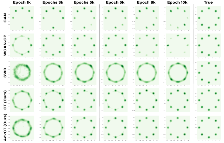
Figure 7: On a 8-Gaussian mixture data, comparison of generation quality and training stability between two min-max deep generative models (DGMs), including vallina GAN and Wasserstein GAN with gradient penalty (WGAN-GP), and two min-max-free DGMs, whose generators are trained under the sliced Wasserstein distance (SWD) and the proposed CT cost, respectively. The critics of GAN, WGAN-GP, the navigators of CT and the adversarially trained feature encoders of AdvCT are fixed after $5k$ training epochs. The last column shows the true data density.

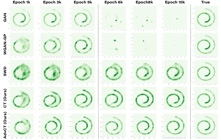
Figure 8: Analogous plot to Fig. 7 for the Swiss-Roll dataset.

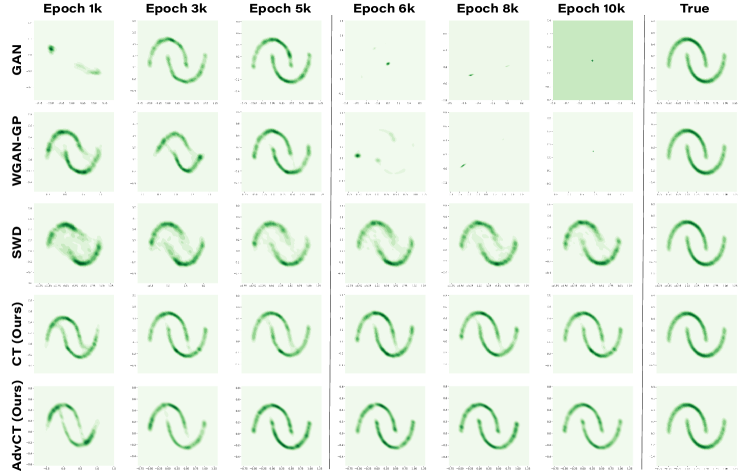
Figure 9: Analogous plot to Fig. 7 for the Half-Moon dataset.

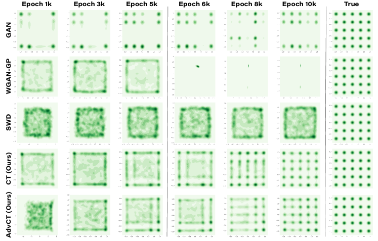
Figure 10: Analogous plot to Fig. 7 for the 25-Gaussian mixture dataset.

E.2 Additional results of cooperative vs. adversarial encoder training

Here we provide additional results to the cooperative experiments, where we minimize CT in the feature encoder spaces trained by: 1) maximizing discriminator loss in GANs, 2) using random slicing projections, 3) maximizing MMD and 4) maximizing CT cost. Fig. 11 shows the results analogous to Fig. 4(a) on other three synthetic datasets: Swiss-Roll, Half-Moon and 25-Gaussian mixture. Fig. 12 provide qualitative results of Table 2 and Table 2.

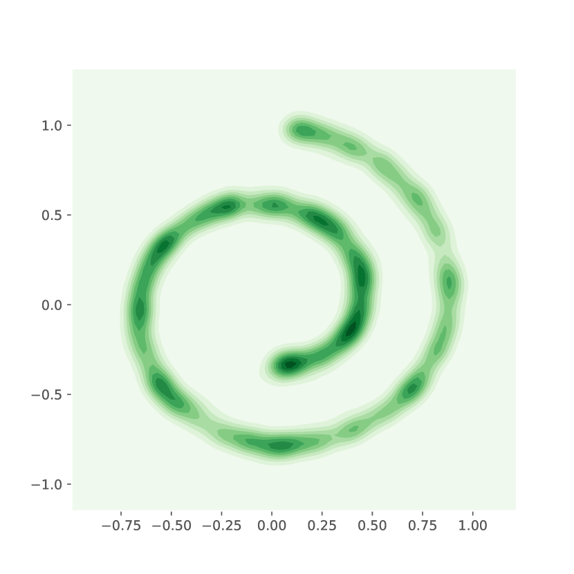
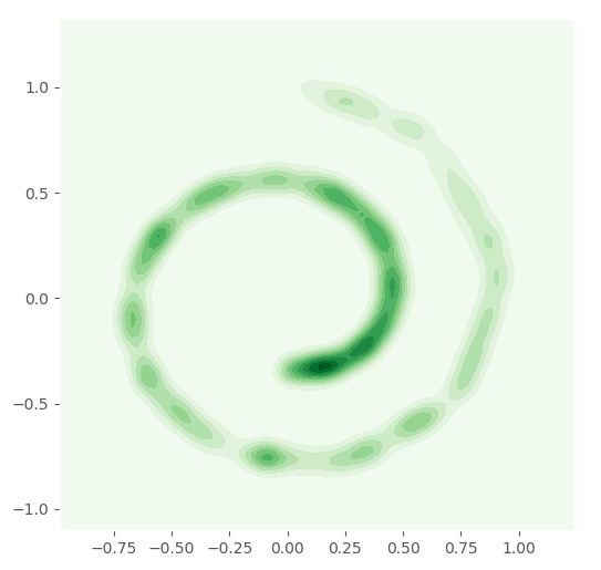
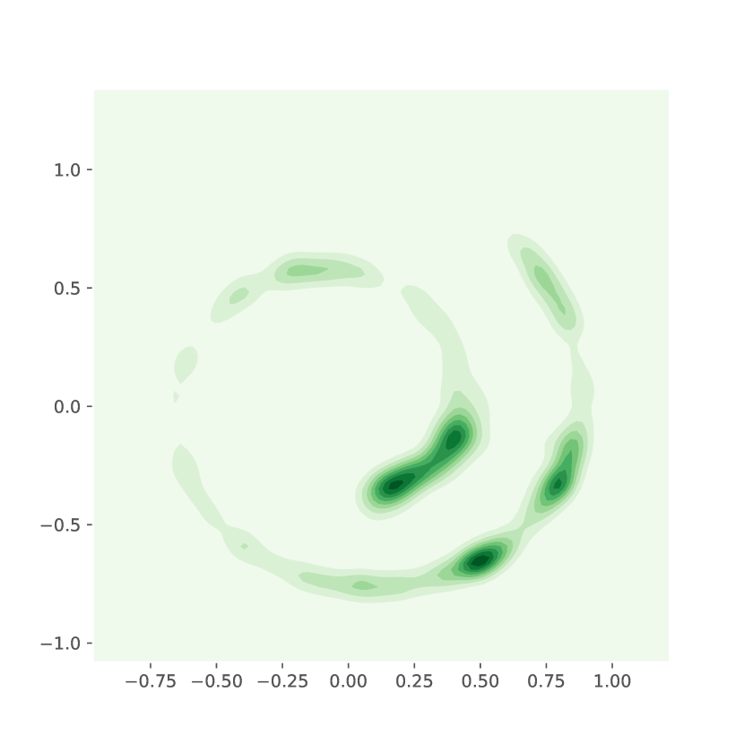
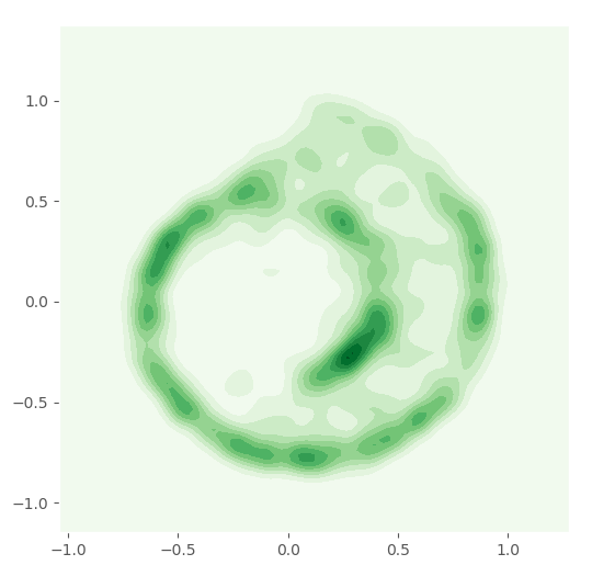
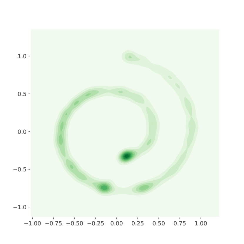
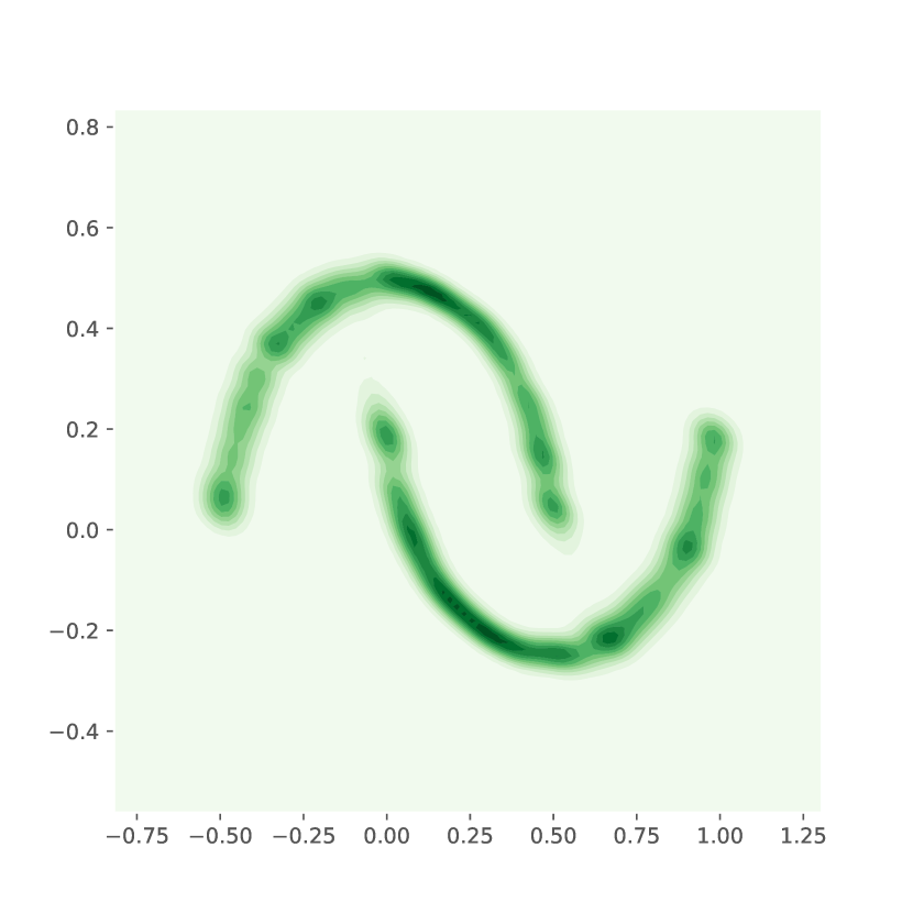
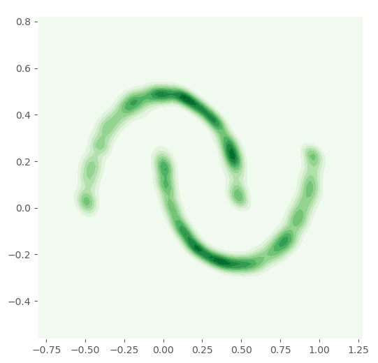
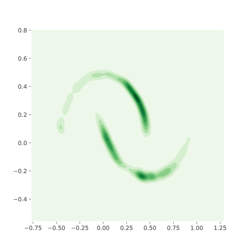
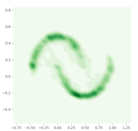
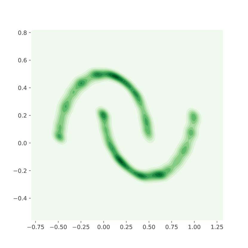
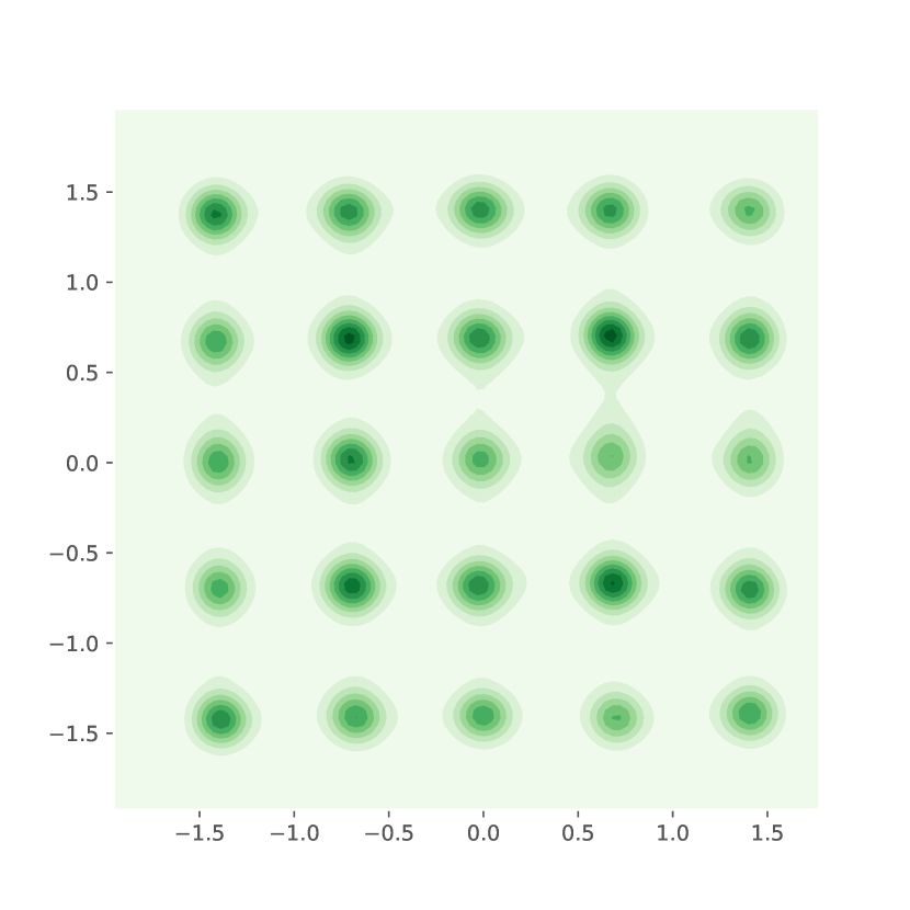
(a) Adv CT.

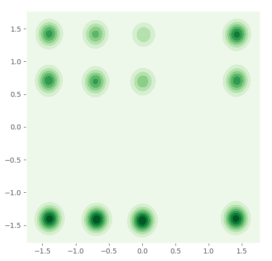
(b) GAN.

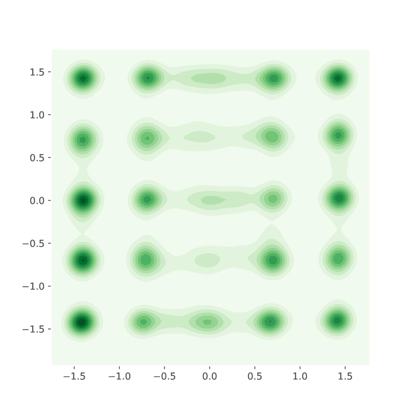
(c) $\mathcal{L}_{D}$ + CT.

(d) SWD.

(e) Slicing + CT.

Figure 11: Analogous plot to Fig. 4(a) on Swiss roll, half-moon and 25 Gaussians datasets. Ablation of fitting results by minimizing CT in different spaces

           

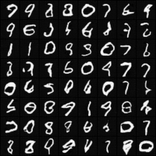
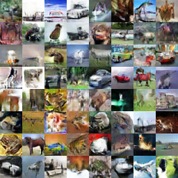
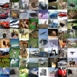
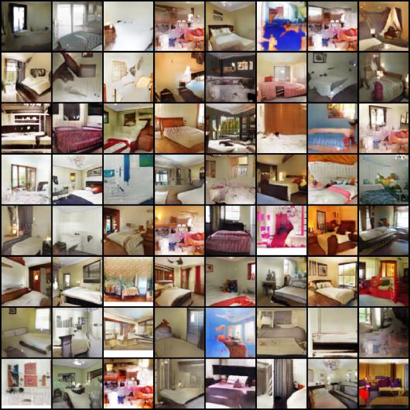
(a) $\mathcal{L}_{D}$ + CT.

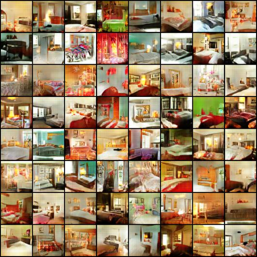
(b) Slicing + CT.

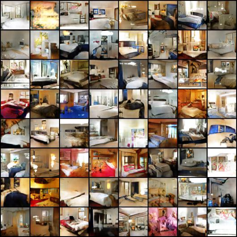
(c) MMD + CT.

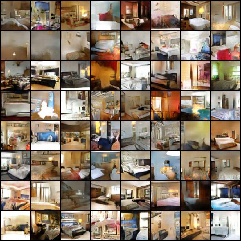
(d) Adv CT.

Figure 12: Analogous plot to Fig. 4(a) and Fig. 11 on image datasets. Ablation of fitting results by minimizing CT in different spaces.

E.3 Empirical Wasserstein loss vs empirical CT

From Table 2, Fig. 4(a), and Fig. 11 we notice the proposed CT can improve the fitting with SWG [70] in the sliced 1D space. Considering SWG applies random slicing projections to project high-dimensional data to several 1D spaces, since the empirical Wasserstein distance has a close form in 1D case and can be calculated with ordered statistics, here we compare the empirical Wasserstein loss and empirical CT cost with a 1D toy experiments.

Let’s consider the same 1D Gaussian mixture data used in Fig. 2, where the bimodal Gaussian mixture has a density form $p_{X}(x)=\frac{1}{4}\mathcal{N}(x;-5,1)+\frac{3}{4}\mathcal{N}(x;2,1)$. We use an empirical sample set $\mathcal{X}$, consisting of $|\mathcal{X}|=5,000$ samples, and train a generative model with the Wasserstein loss and CT cost estimated with these empirical data and generated samples. We vary the training mini-batch size from small to large. Fig. 13 shows the training curve w.r.t. each training epoch and the fitting results with mini-batch size 20, 200 and 5000. We can observe when the mini-batch size $N$ is as large as 5000, both Wasserstein and CT lead to a well-trained generator. However, as shown in the left and middle columns, when $N$ is getting much smaller, the generator trained with Wasserstein under-performs that trained with ACT, especially when the mini-batch size becomes as small as $N=20$. While the Wasserstein distance $\mathcal{W}(X,Y)$ in theory can well guide the training of a generative model, the sample Wasserstein distance $\mathcal{W}(\hat{X}_{N},\hat{Y}_{N})$, whose optimal transport plan is locally re-computed for each mini-batch, could be sensitive to the mini-batch size $N$, which also explains why in practice the SWG are difficult to fit desired distribution. By contrast, CT shows better robustness across mini-batches, leading to a well-trained generator whose performance has low sensitivity to the mini-batch size.

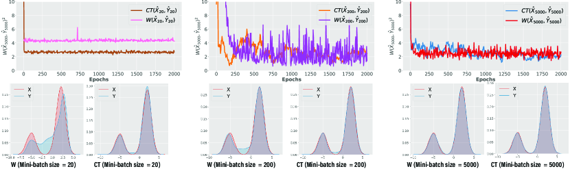
Figure 13: Top: Plot of the sample Wasserstein distance $W_{2}(\hat{X}_{5000},\hat{Y}_{5000})^{2}$ against the number of training epochs, where the generator is trained with either $W_{2}(\hat{X}_{N},\hat{Y}_{N})^{2}$ or the CT cost between $\hat{X}_{N}$ and $\hat{Y}_{N}$, with the mini-batch size set as $N=20$ (left), $N=200$ (middle), or $N=5000$ (right); one epoch consists of $5000/N$ SGD iterations. Bottom: The fitting results of different configurations, where the KDE curves of the data distribution and the generative one are marked in red and blue, respectively.

E.4 Additional results on mode-covering/mode-seeking study

The mode covering and mode seeking behaviors discussed in Figs. 2 also exist in the real image case. For illustration, we use the Stacked-MNIST dataset [66] and fit CT in three configurations: normal, forward only, and backward only. DCGAN [49], VEEGAN [66], PacGAN [71], and PresGAN [72] are applied here as the baseline models to evaluate the mode-capturing capability.

Table 6: Assessing mode collapse on Stacked-MNIST. The true total number of modes is 1,000. DCGAN, VEEGAN, and CT (Backward only) all suffer from collapse. The other models capture nearly all the modes of the data distribution. Furthermore, the distribution of the labels predicted from the images produced by these models is closer to the data distribution, which shows lower KL scores.

Method	Mode Captured	KL
DCGAN [49]	392.0 $\pm$ 7.376	8.012 $\pm$ 0.056
VEEGAN [66]	761.8 $\pm$ 5.741	2.173 $\pm$ 0.045
PacGAN [71]	992.0 $\pm$ 1.673	0.277 $\pm$ 0.005
PresGAN [72]	999.4 $\pm$ 0.80	0.102 $\pm$ 0.003
CT	999.07 $\pm$ 0.162	0.181 $\pm$ 0.003
CT (Foward only)	999.18 $\pm$ 0.9	0.124 $\pm$ 0.003
CT (Backward only)	192 $\pm$ 1.912	9.166 $\pm$ 0.06

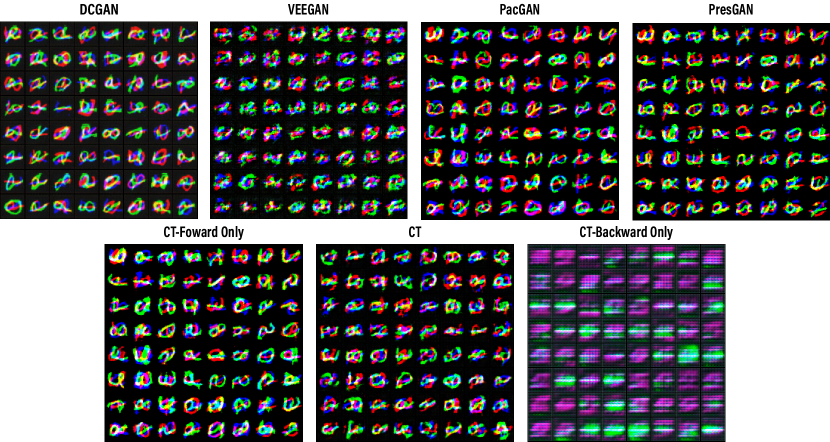
Figure 14: Visual results of the generated samples produced by DCGAN, VEEGAN, PacGAN, PresGAN, and ACT-DCGAN on the Stacked-MNIST dataset.

We calculate the captured mode number of each model, as well as the Kullback–Leibler (KL) divergence of the predicted label distributions between the generated samples and true data samples. For Stacked-MNIST data, there are 1000 modes in total. The results in Table 6 justify CT using only forward or using both forward and backward can almost capture all the modes, thus we do not suffer from the mode collapse problem. Using backward only can only encourages the mode seeking/dropping behavior. Fig. 14 provides the visual justification of this experiment, where the observations is consistent with those on toy datasets: if we only apply forward CT, the generator is encouraged to cover all the modes; if we only apply the backward CT for optimization, we can observe the mode seeking behavior of the generator.

E.5 Additional results on image datasets

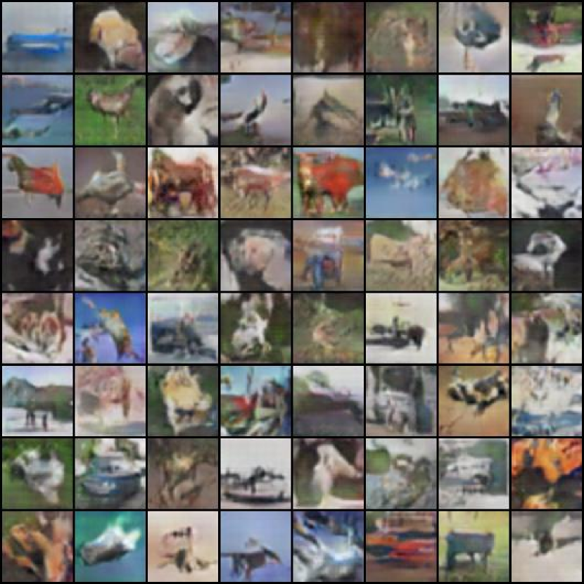
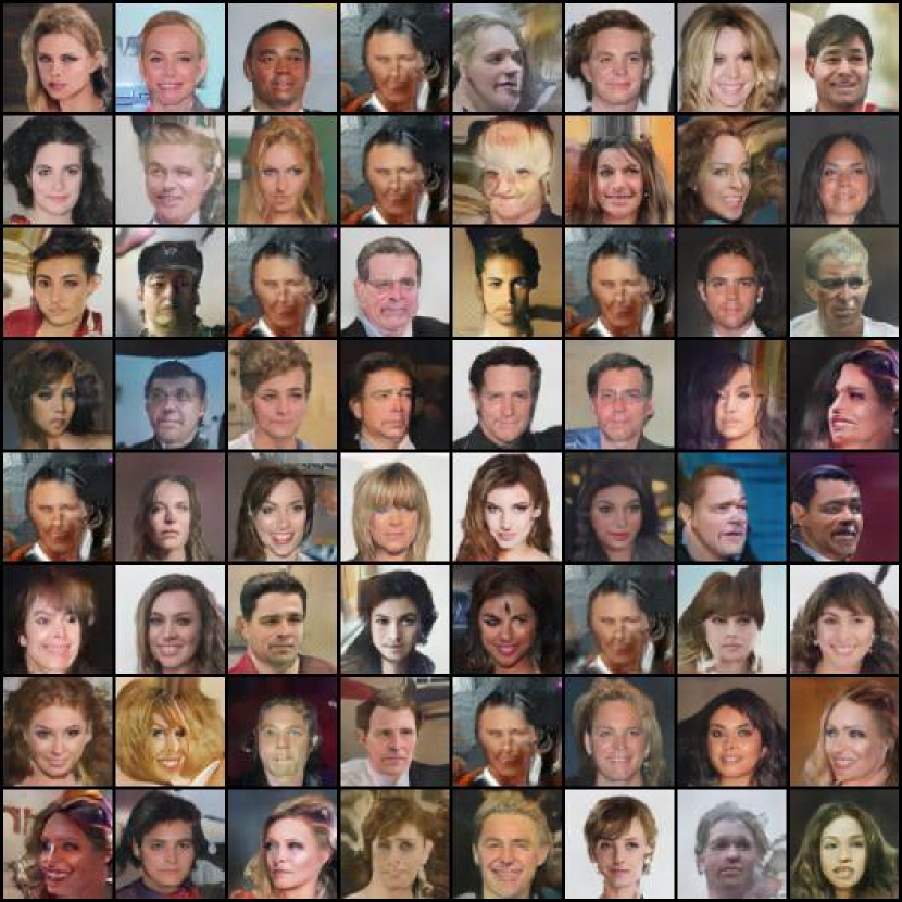
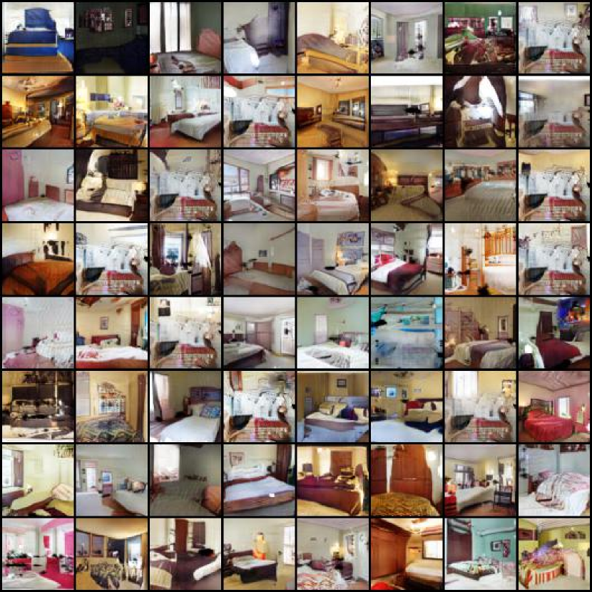
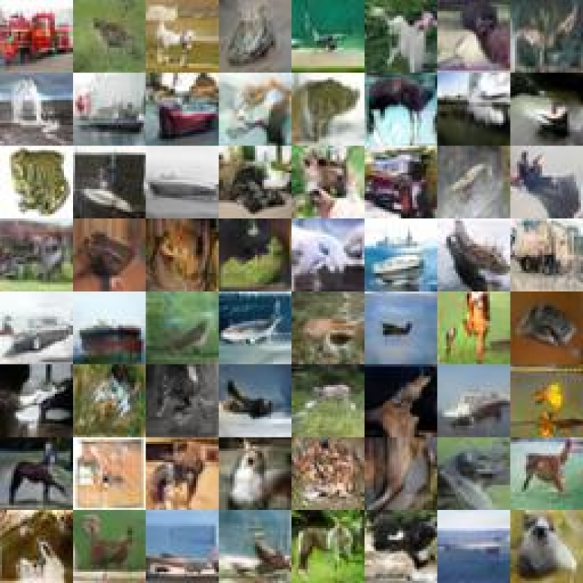
(a) CIFAR-10.

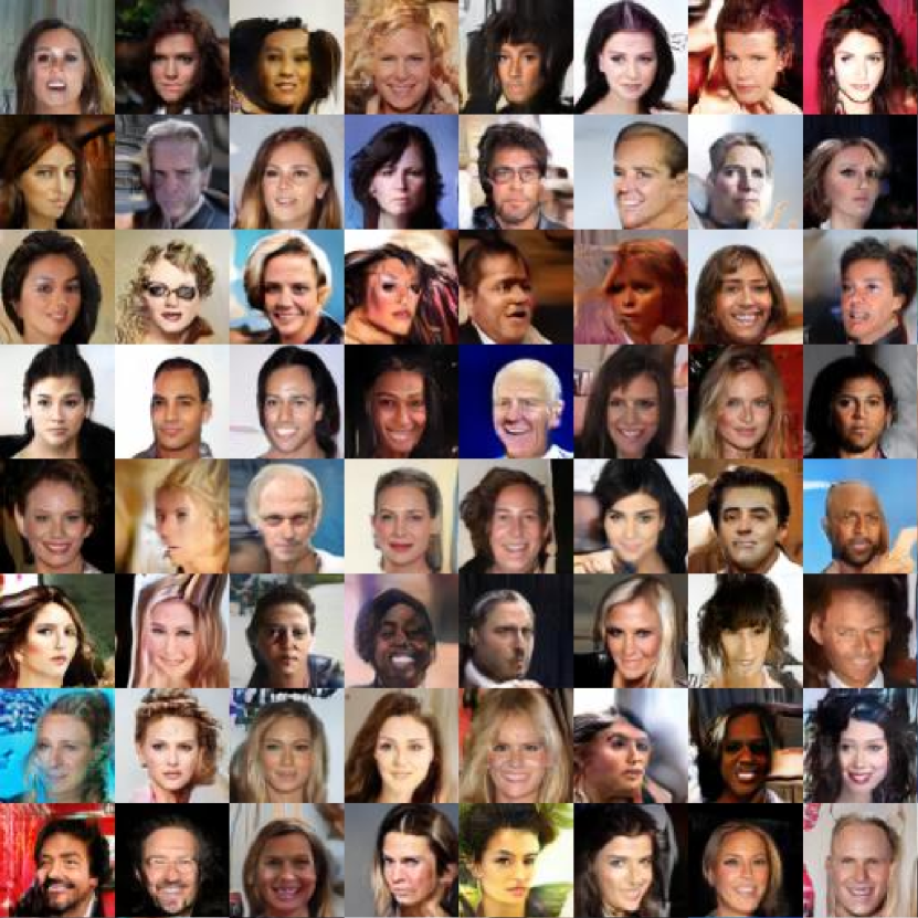
(b) CelebA.

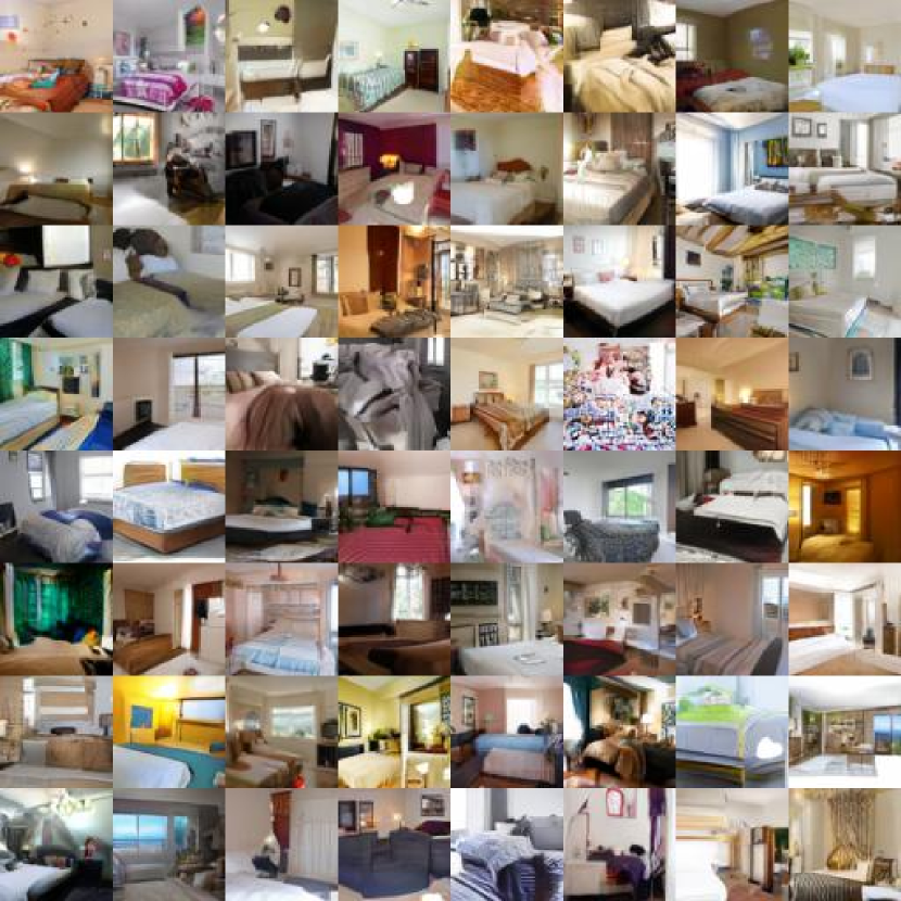
(c) LSUN-Bedroom.

Figure 15: Analogous plot to Fig. 5, with additional generated samples. Top: samples generated with CNN backbone; Bottom: samples generated with ResNet backbone.

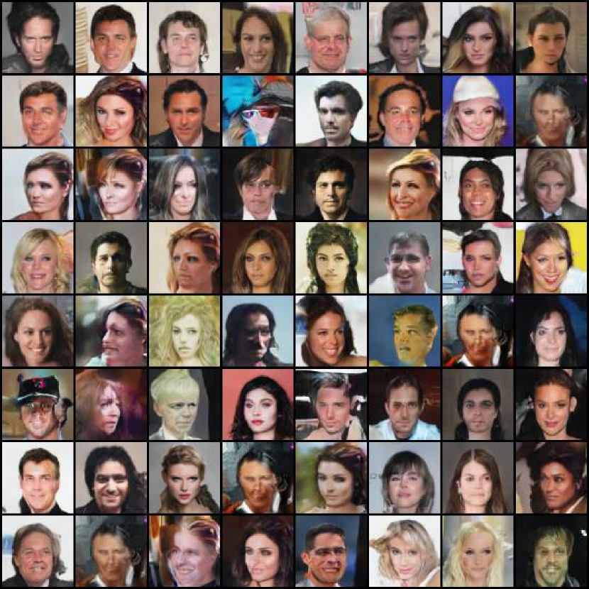
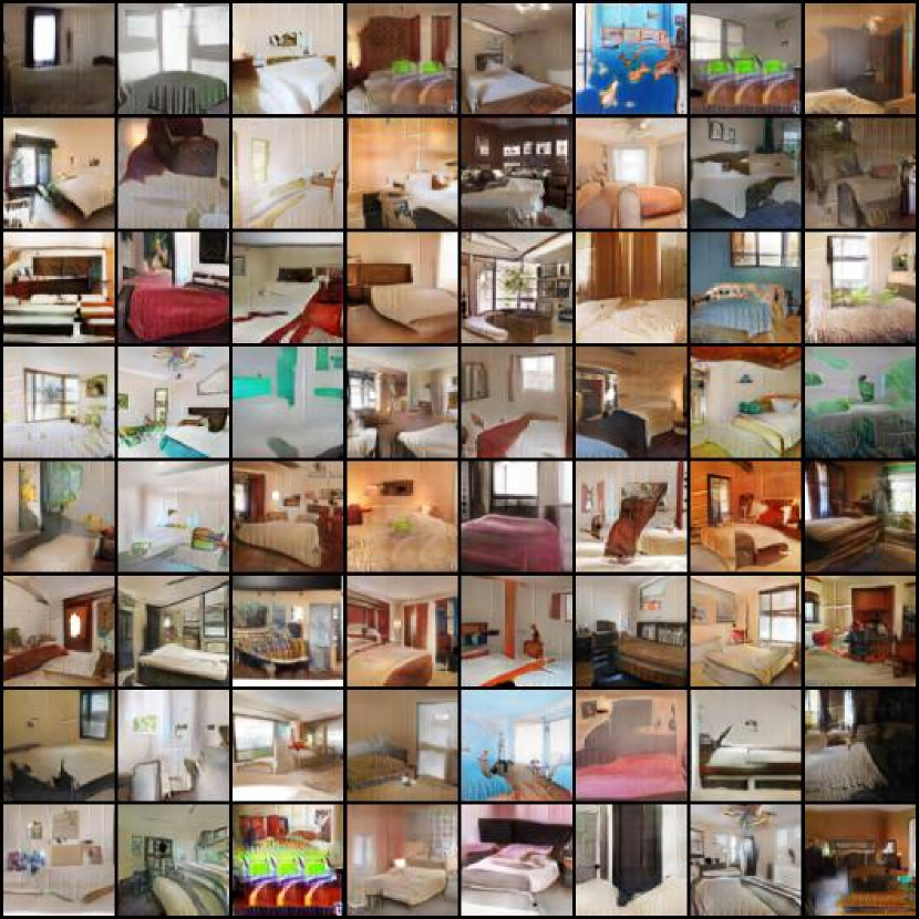
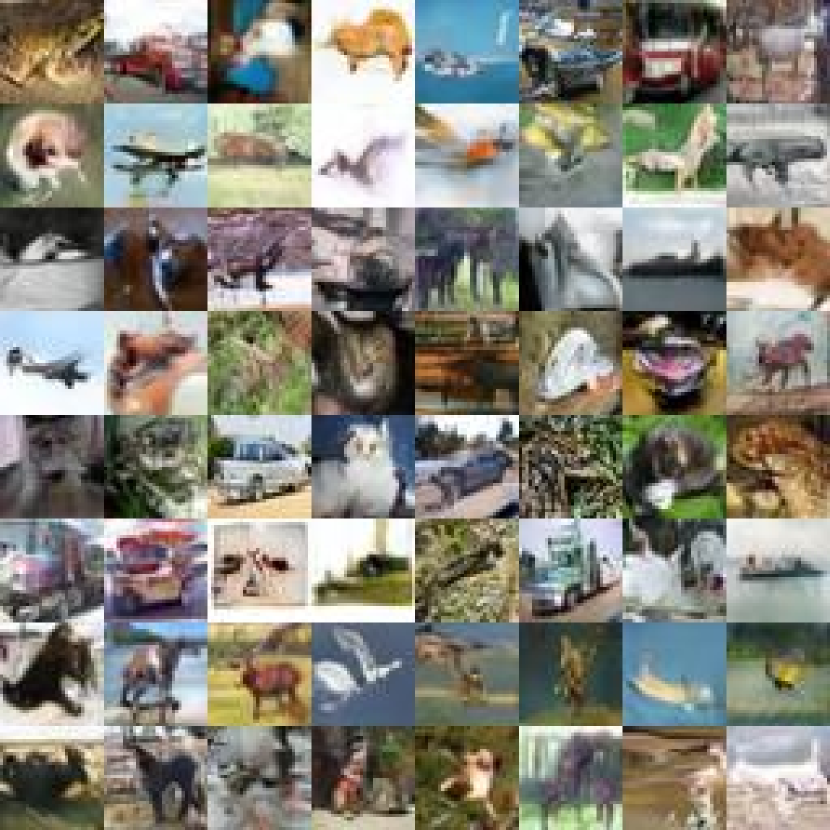
(a) CIFAR-10.

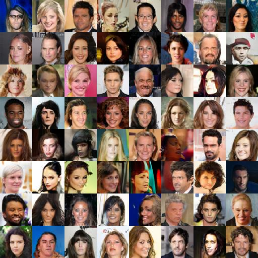
(b) CelebA.

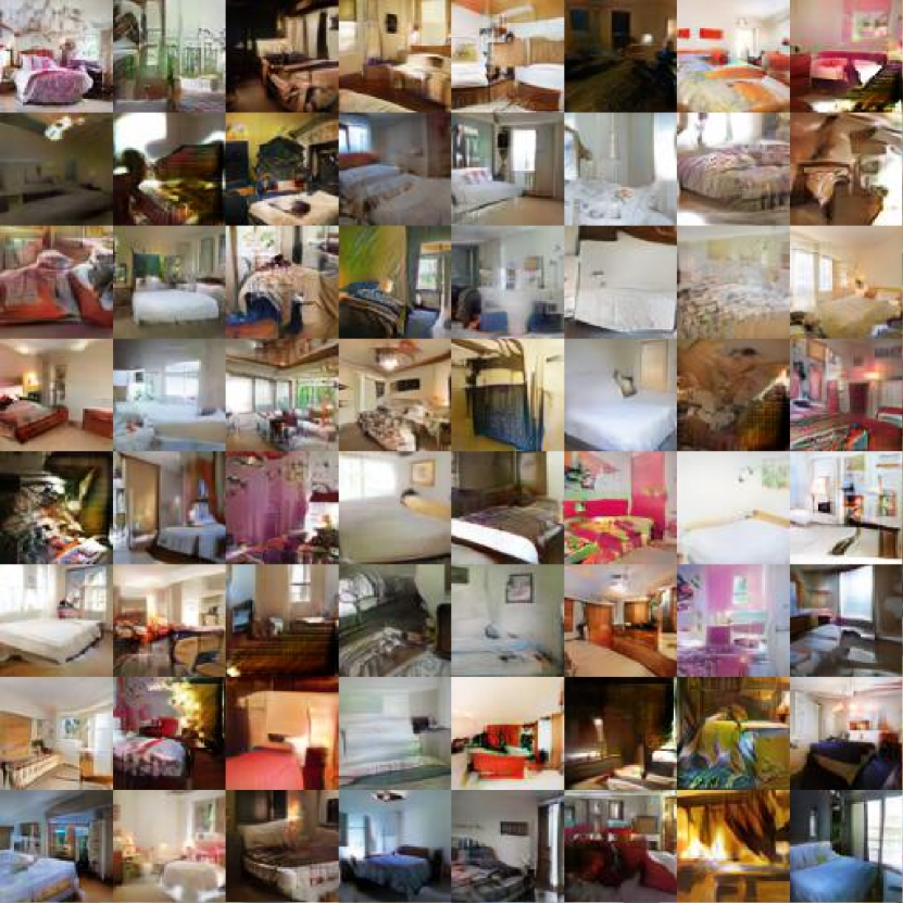
(c) LSUN-Bedroom.

Figure 16: Analogous plot to Fig. 15.

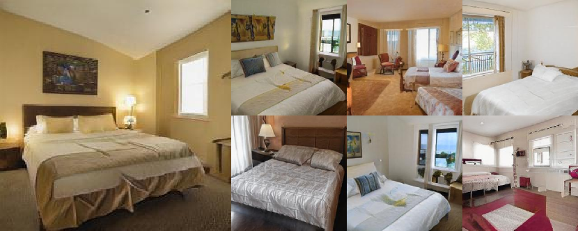
(a) LSUN-Bedroom (256x256).

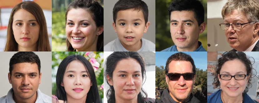
(b) FFHQ (256x256).

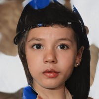
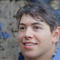
(c) FFHQ (1024x1024).

Figure 17: Analogous plot to Fig. 6: additional high-resolution samples.

Appendix F Architecture summary

Table 7: DCGAN architecture for the CIFAR-10 dataset.

(a) Generator $G_{\boldsymbol{\theta}}$

$\boldsymbol{\epsilon}\in\mathbb{R}^{128}\sim\mathcal{N}(0,1)$
$128\rightarrow 4\times 4\times 512$, dense, linear
$4\times 4$, stride=2 deconv. BN 256 ReLU
$4\times 4$, stride=2 deconv. BN 128 ReLU
$4\times 4$, stride=2 deconv. BN 64 ReLU
$3\times 3$, stride=1 conv. 3 Tanh

(b) Feature encoder $\mathcal{T}_{\boldsymbol{\eta}}$

$\boldsymbol{x}\in{[-1,1]}^{32\times 32\times 3}$
$3\times 3$, stride=1 conv 64 lReLU
$4\times 4$, stride=2 conv 64 lReLU
$3\times 3$, stride=1 conv 128 lReLU
$4\times 4$, stride=2 conv 128 lReLU
$3\times 3$, stride=1 conv 256 lReLU
$4\times 4$, stride=2 conv 256 lReLU
$3\times 3$, stride=1 conv. 512 lReLU
$h\times w\times 512\rightarrow m$, dense, linear

Table 8: DCGAN architecture for the CelebA and LSUN datasets.

(a) Generator $G_{\boldsymbol{\theta}}$

$\boldsymbol{\epsilon}\in\mathbb{R}^{128}\sim\mathcal{N}(0,1)$
$128\rightarrow 4\times 4\times 1024$, dense, linear
$4\times 4$, stride=2 deconv. BN 512 ReLU
$4\times 4$, stride=2 deconv. BN 256 ReLU
$4\times 4$, stride=2 deconv. BN 128 ReLU
$4\times 4$, stride=2 deconv. BN 64 ReLU
$3\times 3$, stride=1 conv. 3 Tanh

(b) Feature encoder $\mathcal{T}_{\boldsymbol{\eta}}$

$\boldsymbol{x}\in{[-1,1]}^{64\times 64\times 3}$
$4\times 4$, stride=2 conv 64 lReLU
$4\times 4$, stride=2 conv BN 128 lReLU
$4\times 4$, stride=2 conv BN 256 lReLU
$3\times 3$, stride=1 conv BN 512 lReLU
$h\times w\times 512\rightarrow m$, dense, linear, Normalize

Table 9: ResNet architecture for the CIFAR-10 dataset.

(a) Generator $G_{\boldsymbol{\theta}}$

$\boldsymbol{\epsilon}\in\mathbb{R}^{128}\sim\mathcal{N}(0,1)$
$128\rightarrow 4\times 4\times 256$, dense, linear
ResBlock up 256
ResBlock up 256
ResBlock up 256
BN, ReLU, $3\times 3$ conv, 3 Tanh

(b) Feature encoder $\mathcal{T}_{\boldsymbol{\eta}}$

$\boldsymbol{x}\in{[-1,1]}^{32\times 32\times 3}$
ResBlock down 128
ResBlock down 128
ResBlock 128
ResBlock 128
ReLU
Global sum pooling
$h=128\rightarrow m$, dense, linear, Normalize

Table 10: ResNet architecture for the CelebA and LSUN datasets.

(a) Generator $G_{\boldsymbol{\theta}}$

$\boldsymbol{\epsilon}\in\mathbb{R}^{128}\sim\mathcal{N}(0,1)$
$128\rightarrow 4\times 4\times 1024$, dense, linear
ResBlock up 512
ResBlock up 256
ResBlock up 128
ResBlock up 64
BN, ReLU, $3\times 3$ conv, 3 Tanh

(b) Feature encoder $\mathcal{T}_{\boldsymbol{\eta}}$

$\boldsymbol{x}\in{[-1,1]}^{64\times 64\times 3}$
ResBlock down 128
ResBlock down 256
ResBlock down 512
ResBlock down 1024
ReLU
Global sum pooling
$h=1024\rightarrow m$, dense, linear, Normalize

Table 11: ResNet architecture for the LSUN-128 dataset.

(a) Generator $G_{\boldsymbol{\theta}}$

$\boldsymbol{\epsilon}\in\mathbb{R}^{128}\sim\mathcal{N}(0,1)$
$128\rightarrow 4\times 4\times 1024$, dense, linear
ResBlock up 1024
ResBlock up 512
ResBlock up 256
ResBlock up 128
ResBlock up 64
BN, ReLU, $3\times 3$ conv, 3 Tanh

(b) Feature encoder $\mathcal{T}_{\boldsymbol{\eta}}$

$\boldsymbol{x}\in{[-1,1]}^{128\times 128\times 3}$
ResBlock down 128
ResBlock down 256
ResBlock down 512
ResBlock down 1024
ResBlock 1024
ReLU
Global sum pooling
$h=1024\rightarrow m$, dense, linear, Normalize

Table 12: ResNet architecture for the CelebA-HQ dataset.

(a) Generator $G_{\boldsymbol{\theta}}$

$\boldsymbol{\epsilon}\in\mathbb{R}^{128}\sim\mathcal{N}(0,1)$
$128\rightarrow 4\times 4\times 1024$, dense, linear
ResBlock up 1024
ResBlock up 512
ResBlock up 512
ResBlock up 256
ResBlock up 128
ResBlock up 64
BN, ReLU, $3\times 3$ conv, 3 Tanh

(b) Feature encoder $\mathcal{T}_{\boldsymbol{\eta}}$

$\boldsymbol{x}\in{[-1,1]}^{256\times 256\times 3}$
ResBlock down 128
ResBlock down 256
ResBlock down 512
ResBlock down 512
ResBlock down 1024
ResBlock 1024
ReLU
Global sum pooling
$h=1024\rightarrow m$, dense, linear, Normalize

References

- Cover [1999] Thomas M Cover. Elements of Information Theory. John Wiley & Sons, 1999.
- Bishop [2006] Christopher M Bishop. Pattern Recognition and Machine Learning. springer, 2006.
- Murphy [2012] Kevin P Murphy. Machine Learning: A Probabilistic Perspective. MIT Press, 2012.
- Kullback and Leibler [1951] Solomon Kullback and Richard A Leibler. On information and sufficiency. The Annals of Mathematical Statistics, 22(1):79–86, 1951.
- Lin [1991] Jianhua Lin. Divergence measures based on the Shannon entropy. IEEE Transactions on Information theory, 37(1):145–151, 1991.
- Gretton et al. [2006] Arthur Gretton, Karsten Borgwardt, Malte Rasch, Bernhard Schölkopf, and Alex Smola. A kernel method for the two-sample-problem. Advances in neural information processing systems, 19:513–520, 2006.
- Kantorovich [2006] Leonid V Kantorovich. On the translocation of masses. Journal of Mathematical Sciences, 133(4):1381–1382, 2006.
- Kingma and Welling [2013] Diederik P Kingma and Max Welling. Auto-encoding variational Bayes. arXiv preprint arXiv:1312.6114, 2013.
- Goodfellow et al. [2014] Ian Goodfellow, Jean Pouget-Abadie, Mehdi Mirza, Bing Xu, David Warde-Farley, Sherjil Ozair, Aaron Courville, and Yoshua Bengio. Generative adversarial nets. In Advances in Neural Information Processing Systems, pages 2672–2680, 2014.
- Bińkowski et al. [2018] Mikołaj Bińkowski, Dougal J. Sutherland, Michael Arbel, and Arthur Gretton. Demystifying MMD GANs. In International Conference on Learning Representations, 2018. URL https://openreview.net/forum?id=r1lUOzWCW.
- Arjovsky et al. [2017] Martin Arjovsky, Soumith Chintala, and Léon Bottou. Wasserstein generative adversarial networks. In Proceedings of the 34th International Conference on Machine Learning-Volume 70, pages 214–223, 2017.
- Genevay et al. [2018] Aude Genevay, Gabriel Peyré, and Marco Cuturi. Learning generative models with Sinkhorn divergences. In International Conference on Artificial Intelligence and Statistics, pages 1608–1617, 2018.
- Balaji et al. [2019] Yogesh Balaji, Hamed Hassani, Rama Chellappa, and Soheil Feizi. Entropic GANs meet VAEs: A statistical approach to compute sample likelihoods in GANs. In International Conference on Machine Learning, pages 414–423, 2019.
- Wainwright and Jordan [2008] Martin J Wainwright and Michael Irwin Jordan. Graphical models, exponential families, and variational inference. Now Publishers Inc, 2008.
- Hoffman et al. [2013] Matthew D Hoffman, David M Blei, Chong Wang, and John Paisley. Stochastic variational inference. The Journal of Machine Learning Research, 14(1):1303–1347, 2013.
- Blei et al. [2017] David M Blei, Alp Kucukelbir, and Jon D McAuliffe. Variational inference: A review for statisticians. Journal of the American statistical Association, 112(518):859–877, 2017.
- Mohamed and Lakshminarayanan [2016] Shakir Mohamed and Balaji Lakshminarayanan. Learning in implicit generative models. arXiv preprint arXiv:1610.03483, 2016.
- Huszár [2017] Ferenc Huszár. Variational inference using implicit distributions. arXiv preprint arXiv:1702.08235, 2017.
- Tran et al. [2017] Dustin Tran, Rajesh Ranganath, and David Blei. Hierarchical implicit models and likelihood-free variational inference. In Advances in Neural Information Processing Systems, pages 5523–5533, 2017.
- Yin and Zhou [2018] Mingzhang Yin and Mingyuan Zhou. Semi-implicit variational inference. In International Conference on Machine Learning, pages 5660–5669, 2018.
- Li et al. [2015] Yujia Li, Kevin Swersky, and Rich Zemel. Generative moment matching networks. In International Conference on Machine Learning, pages 1718–1727, 2015.
- Li et al. [2017] Chun-Liang Li, Wei-Cheng Chang, Yu Cheng, Yiming Yang, and Barnabás Póczos. MMD GAN: Towards deeper understanding of moment matching network. In Advances in Neural Information Processing Systems, pages 2203–2213, 2017.
- Bellemare et al. [2017] Marc G Bellemare, Ivo Danihelka, Will Dabney, Shakir Mohamed, Balaji Lakshminarayanan, Stephan Hoyer, and Rémi Munos. The Cramer distance as a solution to biased Wasserstein gradients. arXiv preprint arXiv:1705.10743, 2017.
- Villani [2008] Cédric Villani. Optimal Transport: Old and New, volume 338. Springer Science & Business Media, 2008.
- Santambrogio [2015] Filippo Santambrogio. Optimal Transport for Applied Mathematicians: Calculus of Variations, PDEs, and Modeling, volume 87. Birkhäuser, 2015.
- Peyré and Cuturi [2019] Gabriel Peyré and Marco Cuturi. Computational optimal transport. Foundations and Trends in Machine Learning, 11(5-6):355–607, 2019.
- Salimans et al. [2018] Tim Salimans, Han Zhang, Alec Radford, and Dimitris Metaxas. Improving GANs using optimal transport. arXiv preprint arXiv:1803.05573, 2018.
- Chen et al. [2017] Xi Chen, Diederik P Kingma, Tim Salimans, Yan Duan, Prafulla Dhariwal, John Schulman, Ilya Sutskever, and Pieter Abbeel. Variational lossy autoencoder. International Conference on Learning Representation, 2017.
- Zhao et al. [2017] Shengjia Zhao, Jiaming Song, and Stefano Ermon. InfoVAE: Information maximizing variational autoencoders. arXiv:1706.02262, 2017.
- Zheng et al. [2018] Huangjie Zheng, Jiangchao Yao, Ya Zhang, and Ivor W Tsang. Degeneration in vae: in the light of fisher information loss. arXiv preprint arXiv:1802.06677, 2018.
- Alemi et al. [2018] Alexander Alemi, Ben Poole, Ian Fischer, Joshua Dillon, Rif A Saurous, and Kevin Murphy. Fixing a broken elbo. In International Conference on Machine Learning, pages 159–168, 2018.
- Zheng et al. [2019] Huangjie Zheng, Jiangchao Yao, Ya Zhang, Ivor W Tsang, and Jia Wang. Understanding vaes in fisher-shannon plane. In Proceedings of the AAAI Conference on Artificial Intelligence, volume 33, pages 5917–5924, 2019.
- Kodali et al. [2017] Naveen Kodali, Jacob Abernethy, James Hays, and Zsolt Kira. On convergence and stability of GANs. arXiv preprint arXiv:1705.07215, 2017.
- Fedus et al. [2018] William Fedus, Mihaela Rosca, Balaji Lakshminarayanan, Andrew M Dai, Shakir Mohamed, and Ian Goodfellow. Many paths to equilibrium: GANs do not need to decrease a divergence at every step. In International Conference on Learning Representations, 2018.
- Stanczuk et al. [2021] Jan Stanczuk, Christian Etmann, Lisa Maria Kreusser, and Carola-Bibiane Schonlieb. Wasserstein GANs work because they fail (to approximate the Wasserstein distance). arXiv preprint arXiv:2103.01678, 2021.
- Iohara et al. [2019] Akihiro Iohara, Takahito Ogawa, and Toshiyuki Tanaka. Generative model based on minimizing exact empirical wasserstein distance, 2019. URL https://openreview.net/forum?id=BJgTZ3C5FX.
- Mallasto et al. [2019] Anton Mallasto, Guido Montúfar, and Augusto Gerolin. How well do WGANs estimate the Wasserstein metric? arXiv preprint arXiv:1910.03875, 2019.
- Pinetz et al. [2019] Thomas Pinetz, Daniel Soukup, and Thomas Pock. On the estimation of the Wasserstein distance in generative models. In German Conference on Pattern Recognition, pages 156–170. Springer, 2019.
- Bottou et al. [2017] Leon Bottou, Martin Arjovsky, David Lopez-Paz, and Maxime Oquab. Geometrical insights for implicit generative modeling. arXiv preprint arXiv:1712.07822, 2017.
- Bernton et al. [2019] Espen Bernton, Pierre E Jacob, Mathieu Gerber, and Christian P Robert. On parameter estimation with the Wasserstein distance. Information and Inference: A Journal of the IMA, 8(4):657–676, 2019.
- Gulrajani et al. [2017] Ishaan Gulrajani, Faruk Ahmed, Martin Arjovsky, Vincent Dumoulin, and Aaron C Courville. Improved training of Wasserstein GANs. In Advances in Neural Information Processing Systems, pages 5767–5777, 2017.
- Deshpande et al. [2018] Ishan Deshpande, Ziyu Zhang, and Alexander G Schwing. Generative modeling using the sliced Wasserstein distance. In Proceedings of the IEEE conference on computer vision and pattern recognition, pages 3483–3491, 2018.
- Wu et al. [2019] Jiqing Wu, Zhiwu Huang, Dinesh Acharya, Wen Li, Janine Thoma, Danda Pani Paudel, and Luc Van Gool. Sliced Wasserstein generative models. In Proceedings of the IEEE conference on computer vision and pattern recognition, pages 3713–3722, 2019.
- Krizhevsky et al. [2009] Alex Krizhevsky et al. Learning multiple layers of features from tiny images. 2009.
- Liu et al. [2015] Ziwei Liu, Ping Luo, Xiaogang Wang, and Xiaoou Tang. Deep learning face attributes in the wild. In Proceedings of the IEEE international conference on computer vision, pages 3730–3738, 2015.
- Yu et al. [2015] Fisher Yu, Ari Seff, Yinda Zhang, Shuran Song, Thomas Funkhouser, and Jianxiong Xiao. LSUN: Construction of a large-scale image dataset using deep learning with humans in the loop. arXiv preprint arXiv:1506.03365, 2015.
- Karras et al. [2018] Tero Karras, Timo Aila, Samuli Laine, and Jaakko Lehtinen. Progressive growing of GANs for improved quality, stability, and variation. In International Conference on Learning Representations, 2018.
- Karras et al. [2019] Tero Karras, Samuli Laine, and Timo Aila. A style-based generator architecture for generative adversarial networks. In Proceedings of the IEEE/CVF Conference on Computer Vision and Pattern Recognition, pages 4401–4410, 2019.
- Radford et al. [2015] Alec Radford, Luke Metz, and Soumith Chintala. Unsupervised representation learning with deep convolutional generative adversarial networks. arXiv preprint arXiv:1511.06434, 2015.
- Miyato et al. [2018] Takeru Miyato, Toshiki Kataoka, Masanori Koyama, and Yuichi Yoshida. Spectral normalization for generative adversarial networks. In International Conference on Learning Representations, 2018.
- Karras et al. [2020a] Tero Karras, Samuli Laine, Miika Aittala, Janne Hellsten, Jaakko Lehtinen, and Timo Aila. Analyzing and improving the image quality of StyleGAN. In Proc. CVPR, 2020a.
- Heusel et al. [2017] Martin Heusel, Hubert Ramsauer, Thomas Unterthiner, Bernhard Nessler, and Sepp Hochreiter. GANs trained by a two time-scale update rule converge to a local Nash equilibrium. In Advances in Neural Information Processing Systems, pages 6626–6637, 2017.
- Salimans et al. [2016] Tim Salimans, Ian Goodfellow, Wojciech Zaremba, Vicki Cheung, Alec Radford, and Xi Chen. Improved techniques for training GANs. In Advances in Neural Information Processing Systems, pages 2234–2242, 2016.
- Szegedy et al. [2016] Christian Szegedy, Vincent Vanhoucke, Sergey Ioffe, Jon Shlens, and Zbigniew Wojna. Rethinking the inception architecture for computer vision. In Proceedings of the IEEE conference on computer vision and pattern recognition, pages 2818–2826, 2016.
- Brock et al. [2018] Andrew Brock, Jeff Donahue, and Karen Simonyan. Large scale GAN training for high fidelity natural image synthesis. arXiv preprint arXiv:1809.11096, 2018.
- Zhang et al. [2019] Han Zhang, Ian Goodfellow, Dimitris Metaxas, and Augustus Odena. Self-attention generative adversarial networks. In International Conference on Machine Learning, pages 7354–7363. PMLR, 2019.
- Armandpour et al. [2021] Mohammadreza Armandpour, Ali Sadeghian, Chunyuan Li, and Mingyuan Zhou. Partition-guided GANs. In Proceedings of the IEEE/CVF Conference on Computer Vision and Pattern Recognition, pages 5099–5109, 2021.
- Zhang et al. [2020] Hao Zhang, Bo Chen, Long Tian, Zhengjue Wang, and Mingyuan Zhou. Variational hetero-encoder randomized GANs for joint image-text modeling. In International Conference on Learning Representations, 2020. URL https://openreview.net/forum?id=H1x5wRVtvS.
- Donahue and Simonyan [2019] Jeff Donahue and Karen Simonyan. Large scale adversarial representation learning. In Advances in Neural Information Processing Systems, pages 10542–10552, 2019.
- Chen et al. [2019] Ting Chen, Xiaohua Zhai, Marvin Ritter, Mario Lucic, and Neil Houlsby. Self-supervised GANs via auxiliary rotation loss. In Proceedings of the IEEE Conference on Computer Vision and Pattern Recognition, pages 12154–12163, 2019.
- Karras et al. [2020b] Tero Karras, Miika Aittala, Janne Hellsten, Samuli Laine, Jaakko Lehtinen, and Timo Aila. Training generative adversarial networks with limited data. arXiv preprint arXiv:2006.06676, 2020b.
- Zhao et al. [2020a] Shengyu Zhao, Zhijian Liu, Ji Lin, Jun-Yan Zhu, and Song Han. Differentiable augmentation for data-efficient GAN training. arXiv preprint arXiv:2006.10738, 2020a.
- Zhao et al. [2020b] Zhengli Zhao, Zizhao Zhang, Ting Chen, Sameer Singh, and Han Zhang. Image augmentations for GAN training. arXiv preprint arXiv:2006.02595, 2020b.
- Song et al. [2021] Yang Song, Jascha Sohl-Dickstein, Diederik P Kingma, Abhishek Kumar, Stefano Ermon, and Ben Poole. Score-based generative modeling through stochastic differential equations. In International Conference on Learning Representations, 2021. URL https://openreview.net/forum?id=PxTIG12RRHS.
- Lecun et al. [1998] Y. Lecun, L. Bottou, Y. Bengio, and P. Haffner. Gradient-based learning applied to document recognition. Proceedings of the IEEE, 86(11):2278–2324, Nov 1998. ISSN 0018-9219. doi: 10.1109/5.726791.
- Srivastava et al. [2017] Akash Srivastava, Lazar Valkov, Chris Russell, Michael U Gutmann, and Charles Sutton. Veegan: Reducing mode collapse in gans using implicit variational learning. In Advances in neural information processing systems, pages 3308–3318, 2017.
- Lee et al. [2020] Cheng-Han Lee, Ziwei Liu, Lingyun Wu, and Ping Luo. Maskgan: Towards diverse and interactive facial image manipulation. In IEEE Conference on Computer Vision and Pattern Recognition (CVPR), 2020.
- Kingma and Ba [2015] Diederik P. Kingma and Jimmy Ba. Adam: A method for stochastic optimization. In Yoshua Bengio and Yann LeCun, editors, 3rd International Conference on Learning Representations, ICLR 2015, San Diego, CA, USA, May 7-9, 2015, Conference Track Proceedings, 2015. URL http://arxiv.org/abs/1412.6980.
- Kolouri et al. [2019] Soheil Kolouri, Kimia Nadjahi, Umut Simsekli, Roland Badeau, and Gustavo Rohde. Generalized sliced Wasserstein distances. In Advances in Neural Information Processing Systems, pages 261–272, 2019.
- Kolouri et al. [2018] Soheil Kolouri, Phillip E Pope, Charles E Martin, and Gustavo K Rohde. Sliced Wasserstein auto-encoders. In International Conference on Learning Representations, 2018.
- Lin et al. [2018] Zinan Lin, Ashish Khetan, Giulia Fanti, and Sewoong Oh. Pacgan: The power of two samples in generative adversarial networks. In Advances in Neural Information Processing Systems, pages 1498–1507, 2018.
- Dieng et al. [2019] Adji B Dieng, Francisco JR Ruiz, David M Blei, and Michalis K Titsias. Prescribed generative adversarial networks. arXiv preprint arXiv:1910.04302, 2019.