Risk-Sensitive Deep RL: Variance-Constrained Actor-Critic Provably Finds Globally Optimal Policy

Abstract

While deep reinforcement learning has achieved tremendous successes in various applications, most existing works only focus on maximizing the expected value of total return and thus ignore its inherent stochasticity. Such stochasticity is also known as the aleatoric uncertainty and is closely related to the notion of risk. In this work, we make the first attempt to study risk-sensitive deep reinforcement learning under the average reward setting with the variance risk criteria. In particular, we focus on a variance-constrained policy optimization problem where the goal is to find a policy that maximizes the expected value of the long-run average reward, subject to a constraint that the long-run variance of the average reward is upper bounded by a threshold. Utilizing Lagrangian and Fenchel dualities, we transform the original problem into an unconstrained saddle-point policy optimization problem, and propose an actor-critic algorithm that iteratively and efficiently updates the policy, the Lagrange multiplier, and the Fenchel dual variable. When both the value and policy functions are represented by multi-layer overparameterized neural networks, we prove that our actor-critic algorithm generates a sequence of policies that finds a globally optimal policy at a sublinear rate. Further, We provide numerical studies of the proposed method using two real datasets to back up the theoretical results.

1 Introduction

Reinforcement learning (RL) is a powerful approach to solving multi-stage decision-making problems by interacting with the environment and learning from experiences. Thanks to the practical efficacy of reinforcement learning, it draws substantial attentions from different communities such as operations research (Bertsekas and Tsitsiklis, 1996; Mertikopoulos and Sandholm, 2016; Wen and Van Roy, 2017; Wang et al., 2017; Zeng et al., 2018), computer science (Sutton and Barto, 1998) and statistics (Menictas et al., 2019; Clifton and Laber, 2020). With the advance of deep learning, over the past few years, we have witnessed phenomenal successes of deep reinforcement learning (DRL) in solving extremely challenging problems such as Go (Silver et al., 2016, 2017; OpenAI, 2019), robotics (Kober et al., 2013; Gu et al., 2017), and natural language processing (Narasimhan et al., 2015), which were once regarded too complicated to be solvable by computer programs in the past.

Despite these empirical successes, providing theoretical justifications for deep reinforcement learning is rather challenging. A significant challenge is that the optimization problems associated with deep reinforcement learning are usually highly nonconvex, which is due to a combination of the following two sources.

First, under the risk-neutral setting, where the goal is to find a policy that maximizes the (long-run) average reward in expectation within a parametric policy class, the optimization objective is a nonconvex function of the policy parameter. This is true even when the policy admits a tabular or linear parameterization, and the global convergence and optimality of policy optimization algorithms for these cases are only established recently. See, e.g., Agarwal et al. (2020); Shani et al. (2020); Mei et al. (2020); Cen et al. (2020) and the references therein.

Second, when the policy is represented by a deep neural network, due to its nonlinearity and complicated structure, policy optimization is significantly more challenging. Theoretical guarantees for deep policy optimization is rather limited. Recently, built upon the theory of neural tangent kernel (Jacot et al., 2018), Liu et al. (2019); Wang et al. (2019); Fu et al. (2020) prove that various actor-critic algorithms with overparameterized neural networks provably achieve global convergence and optimality.

In this paper, going beyond the risk-neutral setting, we make the first attempt to study risk-sensitive deep reinforcement learning. In particular, we focus on the variance risk measure (Sobel, 1982) and aim to find a neural network policy that maximizes the expected value of the long-run average reward under the constraint that the variance of the long-run average reward is upper bounded by a certain threshold. Here the variance constraint incorporates the risk-sensitivity — the reinforcement learning agent is willing to achieve a possibly smaller expected reward in exchange for a smaller variance. Moreover, such a problem is substantially more challenging than the risk-neutral setting and finds important applications. Our goal is to establish an algorithm that provably finds a globally optimal solution to such a risk-sensitive policy optimization problem within the class of deep neural network policies. To the best of our knowledge, this problem has never been considered in existing deep reinforcement learning literature.

1.1 Motivating Applications

Imposing the variance constraint is of substantial practical interests. We provide two concrete motivating applications. The first application is in portfolio management. Reinforcement learning/deep reinforcement learning methods have been applied for portfolio optimization (Moody et al., 1998; Jiang and Liang, 2017), where we dynamically allocate the assets to maximize the total return over time. In such applications, while optimizing the expected total return, it is important to control the volatility/risks of the portfolio. In the celebrated Markowitz model (Markowitz, 1952), it is suggested that the risk of a portfolio is based on the variability/variance of returns, and the model is exactly maximizing the expected total return for a given level of the variance of total return.

The second example is in robotics. It is known that one of the emerging and promising applications of robotics is senior care/medicine (Kohlbacher and Rabe, 2015; Taylor et al., 2016; Tan and Taeihagh, 2020). In these applications, while achieving the maximum expected return, it is extremely important to control the variability of the outcome, as a little change in robotics’ operation could lead to devastating outcomes. While deep reinforcement learning has achieved phenomenal successes in training robotics (Gu et al., 2017; Tai et al., 2017) under the risk-neutral setting, this example shows that risk-sensitive/variance-constrained deep reinforcement indeed calls for a principled solution.

1.2 Major Contribution

Incorporating a variance constraint into deep reinforcement learning raises several challenges. First, this makes the optimization problem a constrained one. Although there are various algorithms designed for constrained Markov decision process (CMDP) (Altman, 1999), these methods cannot be directly applied to our variance-constrained problem. In particular, the constraint in CMDP is irrelevant to the reward function in the objective, whereas the constraint in our problem is the variance of the long-run average reward. Thus, handling such a constraint requires new algorithms. Second, as we employ deep neural network policies, both the expected value and variance of the long-run average reward are highly nonconvex functions of the policy parameter. Third, to obtain the policy update directions, we need to characterize the landscape of the variance of average reward as a functional of the policy. As discussed in Tamar et al. (2016), due to the nonlinearity of the variance of a random variable in the probability space, this raises a substantial challenge even in the simpler linear setting.

To tackle these challenges, inspired by the celebrated actor-critic framework (Konda and Tsitsiklis, 2000), we propose a variance-constrained actor-critic (VARAC) algorithm, where both the policy (actor) and the value functions (critic) are represented by multi-layer overparameterized neural networks. In specific, to handle the first challenge, we transform the constrained problem into an unconstrained saddle point problem via Lagrangian duality. Then, to cope with the third challenge, leveraging Fenchel duality, we further write the variance into the variational form by introducing a dual variable. Thus, the original problem is transformed into a saddle point problem involving the policy $\pi$, Lagrange multiplier $\lambda$, and dual variable $y$. More importantly, when $\lambda$ and $y$ are fixed, the objective is equal to the long-run average of a transformed reward, and thus we can characterize its landscape for policy optimization. For such a saddle point problem, VARAC updates $\pi$, $\lambda$, and $y$ via first-order optimization. Specifically, in each iteration, we update the policy $\pi$ via proximal update with the Kullback-Leibler (KL) divergence serving as the Bregman divergence, while $\lambda$ is updated via (projected) gradient method, and $y$-update step admits a closed-form solution. Moreover, the update directions are all based on the solution to the inner problem of the critic, which corresponds to solving two policy evaluation problems determined by current $\lambda$ and $y$ via temporal-difference learning (Sutton, 1988) with deep neural networks. Our KL-divergence regularized policy update is closely related to the trust-region policy optimization (Schulman et al., 2015) and proximal policy optimization (Schulman et al., 2017), which have demonstrated great empirical successes. Finally, to tackle the second challenge, from a functional perspective, we view the policy update of VARAC as an instantiation of infinite-dimensional mirror descent (Beck and Teboulle, 2003; Zhang and He, 2018), which is well approximated by the parameter update of the policy when the neural network is overparameterized. Thus, we show that under mild assumptions, despite nonconvexity, the policy sequence obtained by VARAC converges to a globally optimal policy at a sublinear $\mathcal{O}(1/\sqrt{K})$ rate, where $K$ is the iteration counter.

In summary, our contribution is two-fold. First, to our best knowledge, we make the first attempt to study risk-sensitive deep reinforcement learning by imposing a variance-based risk constraint. Second, we propose a novel actor-critic algorithm, dubbed as VARAC, which provably finds a globally optimal policy of the variance constrained problem at a sublinear rate. We believe that our work brings a promising future research direction for both optimization and machine learning communities.

1.3 Related Work

Our work extends the field of risk-sensitive optimization. The risks are essentially some measures of the aleatoric uncertainty. In nature, there are two types of uncertainty (Clements et al., 2019). The first type is epistemic uncertainty, which refers to the uncertainty caused by a lack of knowledge and can be reduced by acquiring more data. The second type is aleatoric uncertainty, which refers to the notion of inherent randomness. That is, the uncertainty due to the stochastic nature of the environment, which cannot be reduced even with unlimited data. Optimizing returns while controlling the risk is of great practical importance. Various risk measures are proposed for different applications, which include variance (Rubinstein, 1973), value at risk (VaR) (Pflug, 2000), conditional value at risk (CVaR) (Rockafellar et al., 2000), and utility function (Browne, 1995). The notion of risk is widely studied in the optimization community over past decades. See, e.g., Ruszczyński and Shapiro (2006a, b); Ruszczyński (2010); Dentcheva and Ruszczyński (2019); Kose and Ruszczyński (2020), and the references therein.

Furthermore, our work is closely related to the literature on risk-sensitive reinforcement learning with the variance risk measure. The study of the variance of the total returns in a Markov decision process (MDP) dates back to Sobel (1982). Filar et al. (1989) formulates the variance-regularized MDP as a nonlinear program. Mannor and Tsitsiklis (2011) proves that finding an exact optimal policy of variance-constrained reinforcement learning is NP-hard, even when the model is known. More recently, with linear function approximation, (Tamar et al., 2016) proposes a temporal-difference learning algorithm for estimating the variance of the total reward, and Tamar and Mannor (2013); Prashanth and Ghavamzadeh (2016); Prashanth and Fu (2018) propose actor-critic algorithms for variance-constrained policy optimization. These works all establish asymptotic convergence guarantees via stochastic approximation (Borkar, 2009). A more related work is Xie et al. (2018), which proposes an actor-critic algorithm via Lagrangian and Fenchel duality, which is shown to converge to a stationary point at a sublinear rate under the linear setting. In contrast, our work employs deep neural networks, adopts a different KL-divergence regularized policy update, and our algorithm provably finds a globally optimal policy at a sublinear rate.

Paper Organization. The rest of this paper is organized as follows. In Section 2, we briefly introduce some background knowledge. In Section 3, we present the VARAC algorithm. In Section 4, we provide theoretical guarantees for the VARAC algorithm. To better illustrate our theory, we provide the analysis of VARAC for risk-sensitive RL with linear function approximation in Section 5. In Section 6, we conduct numerical experiments to investigate the empirical performance of our method using two mechanical control environments. We conclude the paper in Section 7.

Notations. For an integer $H$, we denote by $[H]$ the set $\{1,2,\cdots,H\}$. Meanwhile, for any $x\in\mathbb{R}$, we define $[x]_{+}=\max(x,0)$. Furthermore, we denote by $\|\cdot\|_{2}$ the $\ell_{2}$-norm of a vector or the spectral norm of a matrix, and denote by $\|\cdot\|_{\text{F}}$ the Frobenius norm of a matrix. Also, let $\{a_{n}\}_{n\geq 0}$ and $\{b_{n}\}_{n\geq 0}$ be two positive sequences. If there exists some positive constant $c$ such that $\limsup_{n\rightarrow\infty}a_{n}/b_{n}\leq c$, we write $a_{n}=\mathcal{O}(b_{n})$. If $\liminf_{n\rightarrow\infty}a_{n}/b_{n}\geq c_{1}$ for some positive constant $c_{1}$, we write $a_{n}=\Omega(b_{n})$.

2 Background

In this section, we briefly review the Markov Decision Process (MDP) under the average reward setting, the variance-constrained policy optimization problem, and some background of the deep neural network. Markov Decision Process. We consider the Markov decision process $({\mathcal{S}},\mathcal{A},{\mathcal{P}},r)$, where ${\mathcal{S}}$ is a compact state space, $\mathcal{A}$ is a finite action space, ${\mathcal{P}}:{\mathcal{S}}\times{\mathcal{S}}\times\mathcal{A}\to\mathbb{R}$ is the transition kernel, and $r:{\mathcal{S}}\times\mathcal{A}\to\mathbb{R}$ is the reward function. A stationary policy $\pi$ maps each state to a probability distribution over $\mathcal{A}$ that $\pi(\cdot|s)\in{\mathcal{P}}(\mathcal{A})$, where ${\mathcal{P}}(\mathcal{A})$ is the probability simplex on the action space $\mathcal{A}$. Given a policy $\pi$, the state $\{s_{t}\}_{t\geq 0}$ and state-action pair $\{(s_{t},a_{t})\}_{t\geq 0}$ are sampled from the Markov chain over ${\mathcal{S}}$ and ${\mathcal{S}}\times\mathcal{A}$, respectively. Throughout this paper, we assume that the Markov chains induced by any stationary policy admit stationary distributions. Moreover, we denote by $\nu_{\pi}(s)$ and $\sigma_{\pi}(s,a)=\pi(a\,|\,s)\cdot\nu_{\pi}(s)$ the stationary state distribution and the stationary state-action distribution associated with a policy $\pi$, respectively. For ease of presentation, we denote by $\mathbb{E}_{\sigma_{\pi}}[\,\cdot\,]$ and $\mathbb{E}_{\nu_{\pi}}[\,\cdot\,]$ the expectations $\mathbb{E}_{(s,a)\sim\sigma_{\pi}}[\,\cdot\,]=\mathbb{E}_{a\sim\pi(\cdot\,|\,s),s\sim\nu_{\pi}(\cdot)}[\,\cdot\,]$ and $\mathbb{E}_{s\sim\nu_{\pi}}[\,\cdot\,]$, respectively.

Average Reward Setting. For a given stationary policy $\pi:\mathcal{A}\times{\mathcal{S}}\to\mathbb{R}$, we measure its performance using its (long-run) average reward per step, which is defined as

$$\rho(\pi)=\lim_{T\rightarrow\infty}\frac{1}{T}\cdot\mathbb{E}\Bigl{[}\sum_{t=0}^{T-1}r(s_{t},a_{t})\,\big{|}\,\pi\Bigr{]}=\mathbb{E}_{(s,a)\sim\sigma_{\pi}}[r(s,a)].$$ (2.1)

For all states $s$ in ${\mathcal{S}}$ and actions $a$ in $\mathcal{A}$, the differential action-value function (Q-function) of a policy $\pi$ is defined as

$$Q^{\pi}(s,a)=\sum^{\infty}_{t=0}\mathbb{E}\big{[}r(s_{t},a_{t})-\rho(\pi)\,|\,s_{0}=s,~{}a_{0}=a,~{}a_{t}\sim\pi(\cdot\,|\,s_{t}),~{}s_{t+1}\sim{\mathcal{P}}(\cdot\,|\,s_{t},a_{t})\big{]}.$$ (2.2)

Correspondingly, the differential state-value function of a policy $\pi$ is defined as

$$V^{\pi}(s)=\sum^{\infty}_{t=0}\mathbb{E}\big{[}r(s_{t},a_{t})-\rho(\pi)\,|\,s_{0}=s,~{}a_{t}\sim\pi(\cdot\,|\,s_{t}),~{}s_{t+1}\sim{\mathcal{P}}(\cdot\,|\,s_{t},a_{t})\big{]}.$$ (2.3)

In the context of risk-sensitive optimization, one of the most common risk measures is the long-run variance of reward obtained under policy $\pi$, which is defined as

$$\Lambda(\pi)=\lim_{T\rightarrow\infty}\frac{1}{T}\cdot\mathbb{E}\Bigl{[}\sum_{t=0}^{T-1}{\bigl{(}r(s_{t},a_{t})-\rho(\pi)\bigr{)}}^{2}\big{|}\,\pi\Bigr{]}=\mathbb{E}_{(s,a)\sim\sigma_{\pi}}\bigl{[}r(s,a)-\rho(\pi)\bigr{]}^{2}.$$

It is not difficult to show that

$$\Lambda(\pi)=\eta(\pi)-{\rho(\pi)}^{2},\quad\text{where }\,\eta(\pi)=\mathbb{E}_{(s,a)\sim\sigma_{\pi}}[r(s,a)^{2}].$$ (2.4)

Let $W^{\pi}$ and $U^{\pi}$ be the differential action-value and value functions associated with the squared reward of policy $\pi$ that

$$W^{\pi}(s,a) =\sum^{\infty}_{t=0}\mathbb{E}[r(s_{t},a_{t})^{2}-\eta(\pi)\,|\,s_{0}=s,~{}a_{0}=a,~{}a_{t}\sim\pi(\cdot\,|\,s_{t}),~{}s_{t+1}\sim{\mathcal{P}}(\cdot\,|\,s_{t},a_{t})],$$ (2.5)

$$U^{\pi}(s) =\sum^{\infty}_{t=0}\mathbb{E}[r(s_{t},a_{t})^{2}-\eta(\pi)\,|\,s_{0}=s,a_{t}\sim\pi(\cdot\,|\,s_{t}),~{}s_{t+1}\sim{\mathcal{P}}(\cdot\,|\,s_{t},a_{t})].$$ (2.6)

We denote by $\langle\cdot,\cdot\rangle$ the inner product over $\mathcal{A}$, e.g., we have $V^{\pi}(s)=\mathbb{E}_{a\sim\pi(\cdot\,|\,s)}[Q^{\pi}(s,a)]=\langle Q^{\pi}(s,\cdot),\pi(\cdot\,|\,s)\rangle$ and $U^{\pi}(s)=\mathbb{E}_{a\sim\pi(\cdot\,|\,s)}[W^{\pi}(s,a)]=\langle W^{\pi}(s,\cdot),\pi(\cdot\,|\,s)\rangle$.

Throughout our discussion, we impose a standard assumption that the reward function is uniformly bounded. In particular, we assume that there exists a constant $M>0$ such that $M=\sup_{(s,a)\in{\mathcal{S}}\times\mathcal{A}}|r(s,a)|$. As an immediate consequence, we have that for any policy $\pi$,

$$|\rho(\pi)|\leq M,\quad\qquad|\eta(\pi)|\leq M^{2}.$$ (2.7)

Variance-Constrained Problem. We consider the following constrained policy optimization problem to find a policy that maximizes the long-run average reward subject to the constraint that the long-run variance is upper bounded by a certain threshold. In particular, for a given $\alpha>0$, we consider the following constrained optimization problem

$$\max_{\pi}\rho(\pi)\text{ \qquad subject to }\Lambda(\pi)\leq\alpha.$$ (2.8)

Deep Neural Networks. To facilitate our discussion, we briefly review some basics of deep neural networks (DNNs) (Allen-Zhu et al., 2018; Gao et al., 2019). Let $x\in\mathbb{R}^{d}$ be the input data. Suppose that we have a DNN with $H$ layers of width $m$. We denote by $W_{h}$ the weight matrix at the $h$-th layer for $h\in[H]$, where $W_{1}\in\mathbb{R}^{d\times m}$ and $W_{h}\in\mathbb{R}^{m\times m}$ for $2\leq h\leq H$. For a DNN with depth $H$, width $m$, and parameter $\theta=\bigl{(}\mathop{\text{vec}}(W_{1})^{\top},\cdots,\mathop{\text{vec}}(W_{H})^{\top}\bigr{)}^{\top}$, its output $u_{\theta}(x)$ is recursively defined as

$$x^{(0)}=x,$$

$$x^{(h)}=\frac{1}{\sqrt{m}}\cdot\sigma(W_{h}^{\top}x^{(h-1)}),\quad\text{ for }h\in[H],$$ (2.9)

$$u_{\theta}(x)=b^{\top}x^{(H)},$$

where $\sigma(\cdot)=\max\{0,\cdot\}$ is the ReLU activation function, and $b\in\{-1,1\}^{m}$ is the output layer. Without loss of generality, we assume that the input $x\in\mathbb{R}^{d}$ satisfies $\|x\|_{2}=1$, where $\|\cdot\|_{2}$ denotes the $\ell_{2}$-norm. In the context of deep reinforcement learning, this can be achieved by having a known embedding function that maps each state-action pair to the unit sphere in $\mathbb{R}^{d}$. Besides, we initialize the network parameters randomly by

$$[W_{1}]_{i,j}\overset{\rm i.i.d.}{\sim}\mathcal{N}(0,1)\text{ for all }(i,j)\in[d]\times[m],$$

$$[W_{h}]_{i,j}\overset{\rm i.i.d.}{\sim}\mathcal{N}(0,1)\text{ for all }(i,j)\in[m]\times[m]\text{ and }2\leq h\leq H,$$ (2.10)

$$b_{i}\overset{\rm i.i.d.}{\sim}{\rm Unif}(\{-1,1\})\text{ for all }i\in[m].$$

Without loss of generality, we only update $\{W_{h}\}_{h\in[H]}$ throughout the training process, and fix the output layer $b$ as its initialization. We denote by $\theta_{0}=(\mathop{\text{vec}}(W_{1}^{0})^{\top},\cdots,\mathop{\text{vec}}(W_{H}^{0})^{\top})^{\top}$ the initialization of the network parameter. In addition, we restrict network parameter $\theta$ within a ball centered at $\theta_{0}$ with radius $R>0$, which is given by

$${\mathcal{B}}(\theta_{0},R)=\bigl{\{}\theta\in\mathbb{R}^{m_{\rm all}}\colon\|W_{h}-W_{h}^{0}\|_{\text{F}}\leq R\text{ for $h\in[H]$}\bigr{\}},$$ (2.11)

where $\{W_{h}\}_{h\in[H]}$ and $\{W_{h}^{0}\}_{h\in[H]}$ are the weight matrices of network parameters $\theta$ and $\theta_{0}$, respectively, and $\|\cdot\|_{\text{F}}$ denotes the Frobenius norm. For any fixed depth $H$, width $m$, and radius $R>0$, the corresponding class of DNNs is

$$\mathcal{U}(m,H,R)=\bigl{\{}u_{\theta}(\cdot)\colon\theta\in{\mathcal{B}}(\theta_{0},R)\bigr{\}}.$$ (2.12)

3 Algorithm

In this section, we present the Variance-Constrained Actor-Critic with Deep Neural Networks (VARAC) algorithm for solving the variance-constrained problem (2.8).

3.1 Problem Formulation

As we discussed in the introduction, a major challenge of solving problem (2.8) is that the constraint is difficult to handle. We first transform the problem into an unconstrained saddle point problem by employing the Lagrangian dual formulation that

$$\min_{\lambda}\max_{\pi}~{}\rho(\pi)-\lambda\bigl{(}\Lambda(\pi)-\alpha\bigr{)}=\min_{\lambda}\max_{\pi}~{}\rho(\pi)-\lambda\eta(\pi)+\lambda\rho(\pi)^{2}+\lambda\alpha,$$ (3.1)

where the equality follows from (2.4). As mentioned earlier, the quadratic term $\rho(\pi)^{2}$ makes the problem nonlinear in the probability distribution, and raises substantial challenges in the computation. Following Lemma 1 of Xie et al. (2018), we reformulate the problem by leveraging the quadratic term’s Fenchel dual. In particular, by the Fenchel duality, we have that $\rho(\pi)^{2}=\max_{y\in\mathbb{R}}(2y\rho(\pi)-y^{2})$. Then, the Lagrangian dual is transformed to the following form that

$$\min_{\lambda}\max_{\pi}~{}\rho(\pi)-\lambda\eta(\pi)+\lambda\rho(\pi)^{2}+\lambda\alpha$$

$$\qquad=\min_{\lambda}\max_{\pi}~{}\rho(\pi)-\lambda\eta(\pi)+\lambda\max_{y}\bigl{(}-y^{2}+2y\rho(\pi)\bigr{)}+\lambda\alpha$$

$$\qquad=\min_{\lambda}\max_{\pi}\max_{y}~{}(1+2\lambda y)\rho(\pi)-\lambda\eta(\pi)-\lambda y^{2}+\lambda\alpha.$$ (3.2)

To facilitate our discussion, we denote the Lagrangian dual function as

$${\mathcal{L}}(\lambda,\pi,y)=(1+2\lambda y)\rho(\pi)-\lambda\eta(\pi)-\lambda y^{2}+\lambda\alpha.$$ (3.3)

To handle the potentially complicated functional structures, we propose to use DNNs to represent the policy $\pi$, differential action-value function $Q$ defined in (2.2), and differential action-value function $W$ associated with the squared reward defined in (2.5). In particular, we consider the energy-based policy $\pi_{\theta}(a\,|\,s)\propto\exp(\tau^{-1}f_{\theta}(s,a))$, where the energy function $f_{\theta}(s,a)\in\mathcal{U}(m_{\rm a},H_{\rm a},R_{\rm a})$ is parameterized as a DNN with network parameter $\theta$ (Haarnoja et al., 2017; Wang et al., 2019). Also, we assume that $Q(s,a)=Q_{q}(s,a)$ and $W(s,a)=W_{\omega}(s,a)$ for all $(s,a)\in{\mathcal{S}}\times\mathcal{A}$, where $Q_{q}(s,a)\in\mathcal{U}(m_{\rm c},H_{\rm c},R_{\rm c})$ and $W_{\omega}(s,a)\in\mathcal{U}(m_{\rm b},H_{\rm b},R_{\rm b})$ are parameterized as DNNs with network parameters $q$ and $\omega$, respectively.

3.2 VARAC Algorithm

We propose the variance-constrained actor-critic with deep neural networks (VARAC) algorithm to solve (2.8). The algorithm follows the general framework of the actor-critic method (Konda and Tsitsiklis, 2000). This method solves the unconstrained problem of maximizing the long-run average reward in (2.1). At each iteration, in the actor update step, we improve the policy that given the previous estimator for the Q-function, we compute an estimator for the policy gradient, and conduct a gradient step of the policy. In the critic update step, by plugging the updated policy in, we invoke a policy evaluation algorithm to update the estimator for the Q-function.

In our setting, due to the variance constraint, the problem is substantially more challenging, and the actor-critic algorithm cannot be directly applied. As discussed in the previous subsection, by employing the Lagrangian and Fenchel dual formulations, we aim to solve the unconstrained min-max-max problem (3.1). Specifically, at each iteration, we first conduct an actor update step, where we update $\lambda$ and $\pi$. In particular, using solutions from the previous iteration $k$, we update the Lagrangian multiplier $\lambda$ by a projected gradient descent step. Next, we update $\pi_{\theta}$ by the proximal policy optimization (PPO) algorithm (Schulman et al., 2017), where we maximize a KL-penalized objective over $\theta$. To be more specific, in updating $\pi_{\theta}$, by plugging previous estimators for the Q-function in (2.2) and the W-function in (2.5), we aim to maximize a linearized version of ${\mathcal{L}}(\lambda_{k},\pi_{\theta_{k+1}},y_{k})$ over $\theta_{k+1}$ with a penalty of KL-divergence of $\pi_{\theta_{k+1}}$ and $\pi_{\theta_{k}}$, which is equivalent to

$$\max_{\theta_{k+1}}\mathbb{E}_{\nu_{\pi_{\theta_{k}}}}\bigl{[}\bigl{\langle}(1+2{\lambda}_{k}{y}_{k})Q_{q_{k}}(s,\cdot)-{\lambda}_{k}W_{\omega_{k}}(s,\cdot),\pi_{\theta_{k+1}}(\cdot\,|\,s)\bigr{\rangle}-\beta_{k}\cdot{\rm KL}\bigl{(}\pi_{\theta_{k+1}}(\cdot\,|\,s)\,\|\,\pi_{\theta_{k}}(\cdot\,|\,s)\bigr{)}\bigr{]}.$$

The key observation is that, by considering energy-based policies, the problem above admits a tractable solution and can be computed efficiently. Finally, we update $y$ by maximizing a quadratic function.

For the critic update step, we update the estimators for the Q-function and W-function by minimizing the Bellman errors. Recall that we parameterize the Q-function and W-function by deep neural networks with parameters $q$ and $\omega$, respectively. The Bellman error minimization problems become solving

$$\min_{q\in{\mathcal{B}}(q_{0},R_{c})}\mathbb{E}_{\sigma_{k}}[\bigl{(}Q_{q}(s,a)-[{\mathcal{T}}^{\pi_{\theta_{k}}}Q_{q}](s,a)\bigr{)}^{2}],\text{ and }\min_{\omega\in{\mathcal{B}}(\omega_{0},R_{\rm b})}\mathbb{E}_{\sigma_{k}}\big{[}W_{\omega}(s,a)-[\widehat{{\mathcal{T}}}^{\pi_{\theta_{k}}}W_{\omega}](s,a)\big{]}^{2},$$

where ${\mathcal{T}}^{\pi_{\theta_{k}}}$ and $\widehat{{\mathcal{T}}}^{\pi_{\theta_{k}}}$ are Bellman operators defined later in (3.13) and (3.16), respectively. We solve these problems by the temporal difference (TD) method (Sutton, 1988).

We then present the details of the VARAC algorithm. At the $(k-1)$-th iteration, we estimate $\rho(\pi_{\theta_{k}})$ and $\eta(\pi_{\theta_{k}})$ by their sample average estimators that

$$\overline{\rho}(\pi_{\theta_{k}})=\frac{1}{T}\cdot\sum^{T}_{t=1}r(s_{t}^{k},a_{t}^{k}),\qquad\overline{\eta}(\pi_{\theta_{k}})=\frac{1}{T}\cdot\sum^{T}_{t=1}r(s_{t}^{k},a_{t}^{k})^{2},$$ (3.4)

where $T$ is the sample size, and $\{(s_{t}^{k},a_{t}^{k})\}_{t=1}^{T}$ are simulated samples of states and actions following the policy from the previous iteration. In what follows, with some slight abuse of notation, we write $(s_{t}^{k},a_{t}^{k})$ as $(s_{t},a_{t})$. Note that by the boundedness of the reward, we have

$$|\overline{\rho}(\pi_{\theta_{k}})|\leq M,\quad\qquad|\overline{\eta}(\pi_{\theta_{k}})|\leq M^{2}.$$ (3.5)

We then present the actor and critic updates at each iteration.

Actor Update: (i) $\lambda$-Update Step. At the $k$-th iteration, given the solution $(\overline{\lambda}_{k},{\pi}_{\theta_{k}},\overline{y}_{k})$ from the $(k-1)$-th iteration, we compute $\lambda_{k+1}$ using the projected gradient method, where we project the solution onto a bounded region to guarantee the convergence (Prashanth and Ghavamzadeh, 2013, 2016). In particular, we choose a sufficiently large $N>0$ and update $\lambda_{k+1}$ that

$$\lambda_{k+1}=\Pi_{[0,N]}\big{(}\lambda_{k}-\frac{1}{2\gamma_{k}}\partial_{\lambda}{\mathcal{L}}(\lambda_{k},\pi_{\theta_{k}},y_{k})\big{)}=\Pi_{[0,N]}\Big{(}\lambda_{k}-\frac{1}{2\gamma_{k}}\big{(}\alpha+2y_{k}\rho(\pi_{\theta_{k}})-\eta(\pi_{\theta_{k}})-y_{k}^{2}\big{)}\Big{)},$$

where $\gamma_{k}>0$ is some prespecified stepsize. As discussed previously, we do not observe $\rho(\pi_{\theta_{k}})$ and $\eta(\pi_{\theta_{k}})$, and as discussed later in $y$-update step, we do not observe the “ideal” $y_{k}$. Instead, we estimate them using $\overline{\rho}(\pi_{\theta_{k}})$, $\overline{\eta}(\pi_{\theta_{k}})$ in (3.4) and $\overline{y}_{k}$ in (3.11), respectively. We then adopt the following plug-in estimator $\overline{\lambda}_{k+1}$ for the “ideal” $\lambda_{k+1}$ that

$$\overline{\lambda}_{k+1}=\Pi_{[0,N]}\Bigl{(}\overline{\lambda}_{k}-\frac{1}{2\gamma_{k}}\bigl{(}\alpha+2\overline{y}_{k}\overline{\rho}(\pi_{\theta_{k}})-\overline{\eta}(\pi_{\theta_{k}})-\overline{y}_{k}^{2}\bigr{)}\Bigr{)}.$$ (3.6)

(ii) $\pi$-Update Step. Note that the policy $\pi$ is parametrized by $\theta$. By the proximal policy optimization method (Schulman et al., 2017), we update our policy $\pi_{\theta_{k+1}}$ by maximizing the following $\rm{KL}$-penalized objective over $\theta_{k+1}$,

$$\begin{aligned} \max_{\theta_{k+1}}L(\theta_{k+1})=\mathbb{E}_{\nu_{\pi_{\theta_{k}}}}\bigl{[}&\bigl{\langle}(1+2\overline{\lambda}_{k}\overline{y}_{k})Q_{q_{k}}(s,\cdot)-\overline{\lambda}_{k}W_{\omega_{k}}(s,\cdot),\pi_{\theta_{k+1}}(\cdot\,|\,s)\bigr{\rangle}\\ &-\beta_{k}\cdot{\rm KL}\bigl{(}\pi_{\theta_{k+1}}(\cdot\,|\,s)\,\|\,\pi_{\theta_{k}}(\cdot\,|\,s)\bigr{)}\bigr{]},\end{aligned}$$ (3.7)

where $\overline{\lambda}_{k}$ in (3.6) and $\overline{y}_{k}$ in (3.11) are the estimators for $\lambda_{k}$ and $y_{k}$, and $\beta_{k}>0$ is some prespecified penalty parameter. Note that here we use DNNs $Q_{q_{k}}$ and $W_{\omega_{k}}$ to estimate $Q^{\pi_{\theta_{k}}}$ and $W^{\pi_{\theta_{k}}}$, and we provide the theoretical justifications of using DNNs in Section 4.2.

Solving problem (3.7) is challenging since the gradient of KL-divergence in the objective is difficult to derive. To efficiently and approximately solve the maximization problem (3.7), we consider the energy-based policy $\pi_{\theta_{k+1}}\propto\exp(\tau_{k+1}^{-1}f_{\theta_{k+1}})$, where $\tau_{k+1}>0$ is a temperature parameter, and $f_{\theta}(s,a)\in\mathcal{U}(m_{\rm a},H_{\rm a},R_{\rm a})$, which is parameterized by a DNN with network parameter $\theta$, is an energy function (Liu et al., 2019). The next proposition shows that problem (3.7) admits a tractable solution of the oracle infinite-dimensional policy update.

Proposition 3.1.

Let $\pi_{\theta_{k+1}}\propto\exp(\tau_{k+1}^{-1}f_{\theta_{k+1}})$ be an energy-based policy. For any given $\overline{\lambda}_{k}$ and $\overline{y}_{k}$, and given estimators $Q_{q_{k}}$, $W_{\omega_{k}}$ for $Q^{\pi_{\theta_{k}}}$ and $W^{\pi_{\theta_{k}}}$ respectively, we have that $\widehat{\pi}_{k+1}=\mathop{\mathrm{argmax}}_{\pi}(\mathbb{E}_{\nu_{k}}[\langle(1+2\overline{\lambda}_{k}\overline{y}_{k})Q_{q_{k}}(s,\cdot)-\overline{\lambda}_{k}W_{\omega_{k}}(s,\cdot),\pi(\cdot\,|\,s)\rangle-\beta_{k}\cdot{\rm KL}(\pi(\cdot\,|\,s)\,\|\,\pi_{\theta_{k}}(\cdot\,|\,s))])$ satisfies

$$\widehat{\pi}_{k+1}\propto\exp\big{(}\beta_{k}^{-1}(1+2\overline{\lambda}_{k}\overline{y}_{k})Q_{q_{k}}-\beta_{k}^{-1}\overline{\lambda}_{k}W_{\omega_{k}}+\tau_{k}^{-1}f_{\theta_{k}}\big{)},$$ (3.8)

where $\nu_{k}=\nu_{\pi_{\theta_{k}}}$ is the stationary state distribution generated by $\pi_{\theta_{k}}.$

Proof.

See Appendix B for the detailed proof. ∎

By Proposition 3.1, we update the policy parameter $\theta$ by solving the following problem,

$$\theta_{k+1}=\mathop{\mathrm{argmin}}_{\theta\in{\mathcal{B}}(\theta_{0},R_{a})}\mathbb{E}_{{\sigma}_{k}}\bigl{[}\bigl{(}f_{\theta}(s,a)-\tau_{k+1}\cdot(\beta_{k}^{-1}(1+2\overline{\lambda}_{k}\overline{y}_{k})Q_{q_{k}}-\beta_{k}^{-1}\overline{\lambda}_{k}W_{\omega_{k}}+\tau^{-1}_{k}f_{\theta_{k}}(s,a))\bigr{)}^{2}\bigr{]},$$ (3.9)

where $\sigma_{k}$ is the stationary state-action distribution of $\pi_{\theta_{k}}$. That is, to minimize the distance between the output $f_{\theta_{k+1}}$ and the right hand side of (3.9). To solve (3.9), we adopt the projected stochastic gradient descent method. Specifically, given an initial $\theta_{0}$, at the $t$-th iteration, we update

$$\theta{(t+1)}\leftarrow\Pi_{{\mathcal{B}}(\theta_{0},R_{a})}\Bigl{(} \theta{(t)}-\zeta\cdot\bigl{(}f_{\theta{(t)}}(s,a)-\tau_{k+1}\cdot\big{(}\beta_{k}^{-1}(1+2\overline{\lambda}_{k}\overline{y}_{k})Q_{q_{k}}$$ (3.10)

$$+\beta_{k}^{-1}\overline{\lambda}_{k}W_{\omega_{k}}+\tau^{-1}_{k}f_{\theta_{k}}(s,a)\big{)}\bigr{)}\cdot\nabla_{\theta}f_{\theta{(t)}}(s,a)\Bigr{)},$$

where the operator $\Pi_{{\mathcal{B}}(\theta_{0},R_{a})}(\cdot)$ projects the solution onto the set ${\mathcal{B}}(\theta_{0},R_{a})$ defined in (2.11), the state-action pair $(s,a)$ is sampled from $\sigma_{k}=\sigma_{\pi_{\theta_{k}}}$, and $\zeta>0$ is the stepsize. See Algorithm 2 in Appendix A for a pseudocode.

(iii) $y$-Update Step. Given $\overline{\lambda}_{k+1}$ and $\theta_{k+1}$, we update $y_{k+1}=\mathop{\mathrm{argmax}}_{y}{\mathcal{L}}(\overline{\lambda}_{k+1},\pi_{\theta_{k+1}},y)$. By the property of the quadratic function, it is easy to see that $y_{k+1}=\rho(\pi_{\theta_{k+1}})$. However, since $\rho(\pi_{\theta_{k+1}})$ is unknown, we adopt $\overline{\rho}(\pi_{\theta_{k+1}})$ defined in (3.4) as an estimator for $y_{k+1}$ that

$$\overline{y}_{k+1}=\overline{\rho}(\pi_{\theta_{k+1}}).$$ (3.11)

Critic Update: (i) $q$-Update Step. In the critic update, we evaluate the current solution $(\overline{\lambda}_{k},\pi_{\theta_{k}},\overline{y}_{k})$ by estimating the corresponding value functions. We first consider the differential action-value function (Q-function), and derive an estimator $Q_{q_{k}}$ for $Q^{\pi_{\theta_{k}}}$ in (3.7), where $Q_{q_{k}}$ is parametrized as a DNN with network parameter $q_{k}$. To obtain $q_{k}$, we solve the following least-squares problem

$$q_{k}=\mathop{\mathrm{argmin}}_{q\in{\mathcal{B}}(q_{0},R_{c})}\mathbb{E}_{\sigma_{k}}[\bigl{(}Q_{q}(s,a)-[{\mathcal{T}}^{\pi_{\theta_{k}}}Q_{q}](s,a)\bigr{)}^{2}],$$ (3.12)

where $\sigma_{k}$ is the stationary state-action distribution of the policy $\pi_{\theta_{k}}$. Here the Bellman operator ${\mathcal{T}}^{\pi}$ of a policy $\pi$ is

$$[{\mathcal{T}}^{\pi}Q](s,a)=\mathbb{E}[r(s,a)-\rho(\pi)+Q(s^{\prime},a^{\prime})\,\big{|}\,s^{\prime}\sim{\mathcal{P}}(\cdot\,|\,s,a),~{}a^{\prime}\sim\pi(\cdot\,|\,s^{\prime})].$$ (3.13)

Recall that $Q_{q}\in{\mathcal{U}}(m_{c},H_{c},R_{c})$ is defined through a deep neural network in (2.12), where $q$ is the network parameter, $H_{c}$ is the depth, $m_{c}$ is the width, and $R_{c}$ is the projection radii. To solve (3.12), given an initial $q_{0}$, we use the iterative TD-update that at the $t$-th iteration, we let

$$q{(t+1)}\leftarrow\Pi_{{\mathcal{B}}{(q_{0},R_{\rm c})}}\Bigl{(} q{(t)}-\delta\cdot\bigl{(}Q_{q{(t)}}(s,a)-r(s,a)$$ (3.14)

$$+\overline{\rho}(\pi_{\theta_{k}})-Q_{q{(t)}}(s^{\prime},a^{\prime})\bigr{)}\cdot\nabla_{q}Q_{q{(t)}}(s,a)\Bigr{)},$$

where $(s,a)\sim\sigma_{k}$, $s^{\prime}\sim{\mathcal{P}}(\cdot\,|\,s,a)$, $a^{\prime}\sim\pi_{\theta_{k}}(\cdot\,|\,s^{\prime})$, and $\delta$ is the stepsize. See Algorithm 3 in Appendix A for a pseudocode.

(ii) $\omega$-Update Step. Next, we derive an estimator $W_{\omega_{k}}$ for $W^{\pi_{\theta_{k}}}$ in (3.7). The procedure is similar to the previous step. We solve the following least-squares problem to obtain $\omega_{k}$,

$$\omega_{k}=\mathop{\mathrm{argmin}}_{\omega\in{\mathcal{B}}(\omega_{0},R_{\rm b})}\mathbb{E}_{\sigma_{k}}\big{[}W_{\omega}(s,a)-[\widehat{{\mathcal{T}}}^{\pi_{\theta_{k}}}W_{\omega}](s,a)\big{]}^{2},$$ (3.15)

where the operator $\widehat{{\mathcal{T}}}^{\pi}$ of a policy $\pi$ is defined as

$$[\widehat{{\mathcal{T}}}^{\pi}W](s,a)=\mathbb{E}[r(s,a)^{2}-\eta(\pi)+W(s^{\prime},a^{\prime})\,\big{|}\,s^{\prime}\sim{\mathcal{P}}(\cdot\,|\,s,a),~{}a^{\prime}\sim\pi(\cdot\,|\,s^{\prime})].$$ (3.16)

As we discussed earlier, we parameterize $W$ using a DNN that we let $W_{\omega}\in{\mathcal{U}}(m_{b},H_{b},R_{b})$ defined in (2.12), where $\omega$ is the network parameter, $H_{b}$ is the depth, $m_{b}$ is the width, and $R_{b}$ is the projection radii. To solve (3.15), given an initial $\omega_{0}$, we use the TD update that at the $t$-th iteration, we let

$$\omega{(t+1)}\leftarrow\Pi_{{\mathcal{B}}{(\omega_{0},R_{b})}}\Bigl{(} \omega{(t)}-\delta\cdot\bigl{(}W_{\omega(t)}(s,a)-r(s,a)^{2}$$ (3.17)

$$+\overline{\eta}(\pi_{\theta_{k}})-W_{\omega{(t)}}(s^{\prime},a^{\prime})\bigr{)}\cdot\nabla_{\omega}W_{\omega{(t)}}(s,a)\Bigr{)},$$

where $(s,a)\sim\sigma_{k}$, $s^{\prime}\sim{\mathcal{P}}(\cdot\,|\,s,a)$, $a^{\prime}\sim\pi_{\theta_{k}}(\cdot\,|\,s^{\prime})$, and $\delta$ is the stepsize. See Algorithm 4 in Appendix A for a pseudocode.

Putting the actor and critic updates together, we present the pseudocode of the VARAC algorithm in Algorithm 1.

Algorithm 1 Variance-Constrained Actor-Critic with Deep Neural Networks

0:  MDP $({\mathcal{S}},\mathcal{A},{\mathcal{P}},r)$, penalty parameter $\beta$, widths $m_{a}$, $m_{b}$ and $m_{c}$, depths $H_{a}$, $H_{b}$ and $H_{c}$, projection radii $R_{a}$, $R_{b}$ and $R_{c}$, number of SGD and TD iterations $T$ and number of VARAC iterations $K$

1:  Initialize with uniform policy: $\tau_{0}\leftarrow 1$, $f_{\theta_{0}}\leftarrow 0$, $\pi_{\theta_{0}}\leftarrow\pi_{0}\propto\exp(\tau_{0}^{-1}f_{\theta_{0}})$

2:  Sample $\{(s_{t},a_{t},a^{0}_{t},s_{t}^{\prime},a_{t}^{\prime})\}^{T}_{t=1}$ with $(s_{t},a_{t})\sim\sigma_{0}$, $a^{0}_{t}\sim\pi_{0}(\cdot\,|\,s_{t})$, $s_{t}^{\prime}\sim{\mathcal{P}}(\cdot\,|\,s_{t},a_{t})$ and $a_{t}^{\prime}\sim\pi_{\theta_{0}}(\cdot\,|\,s_{t}^{\prime})$

3:  Estimate $\rho(\pi_{\theta_{0}})$ and $\eta(\pi_{\theta_{0}})$ by $\overline{\rho}(\pi_{\theta_{0}})=\frac{1}{T}\cdot\sum^{T}_{t=1}r(s_{t},a_{t})$ and $\overline{\eta}(\pi_{\theta_{0}})=\frac{1}{T}\cdot\sum^{T}_{t=1}r(s_{t},a_{t})^{2}$

4:  for $k=0,\dots,K-1$ do

5:     Set temperature parameter $\tau_{k+1}\leftarrow\beta\sqrt{K}/(k+1)$ and penalty parameter $\beta_{k}\leftarrow\beta\sqrt{K}$

6:     Solve $Q_{q_{k}}(s,a)\in\mathcal{U}(m_{\rm c},H_{\rm c},R_{\rm c})$ in (3.12) using the TD update in (3.14) (Algorithm 3)

7:     Solve $W_{\omega_{k}}(s,a)\in\mathcal{U}(m_{\rm b},H_{\rm b},R_{\rm b})$ in (3.15) using the TD update in (3.17) (Algorithm 4)

8:     Update $\lambda$ : $\overline{\lambda}_{k+1}=\Pi_{[0,N]}\bigl{(}\overline{\lambda}_{k}-\frac{1}{2\gamma_{k}}(\alpha+2\overline{y}_{k}\overline{\rho}(\pi_{\theta_{k}})-\overline{\eta}(\pi_{\theta_{k}})-\overline{y}_{k}^{2})\bigr{)}$

9:     Solve $f_{\theta_{k+1}}\in\mathcal{U}(m_{\rm a},H_{\rm a},R_{\rm a})$ in (3.9) using the SGD update in (3.10) (Algorithm 2)

10:     Update policy: $\pi_{\theta_{k+1}}\propto\exp(\tau_{k+1}^{-1}f_{\theta_{k+1}})$

11:     Sample $\{(s_{t},a_{t},a^{0}_{t},s_{t}^{\prime},a_{t}^{\prime})\}^{T}_{t=1}$ with $(s_{t},a_{t})\sim\sigma_{k+1}$, $a^{0}_{t}\sim\pi_{0}(\cdot\,|\,s_{t})$, $s_{t}^{\prime}\sim{\mathcal{P}}(\cdot\,|\,s_{t},a_{t})$ and $a_{t}^{\prime}\sim\pi_{\theta_{k+1}}(\cdot\,|\,s_{t}^{\prime})$

12:     Estimate $\rho(\pi_{\theta_{k+1}})$ and $\eta(\pi_{\theta_{k+1}})$ by $\overline{\rho}(\pi_{\theta_{k+1}})=\frac{1}{T}\cdot\sum^{T}_{t=1}r(s_{t},a_{t})$ and $\overline{\eta}(\pi_{\theta_{k+1}})=\frac{1}{T}\cdot\sum^{T}_{t=1}r(s_{t},a_{t})^{2}$

13:     Update $y$ : $\overline{y}_{k+1}=\overline{\rho}(\pi_{\theta_{k+1}})$

14:  end for

4 Theoretical Results

In this section, we establish the convergence of the proposed VARAC algorithm by analyzing the estimation and computation errors, and we show that the solution converges to a globally optimal solution at an $\mathcal{O}(1/\sqrt{K})$ rate. Further, we show that under the Slater condition, we have both optimality and feasibility gaps diminish at $\mathcal{O}(1/\sqrt{K})$ rates. Before going further, we first impose some mild assumptions.

Assumption 4.1.

There exists a saddle point $(\lambda^{*},\pi^{*},y^{*})$, which is a solution of the saddle point optimization problem (3.1).

Assumption 4.2.

For any $Q_{q}\in\mathcal{U}(m_{\rm c},H_{\rm c},R_{\rm c})$, $W_{\omega}\in\mathcal{U}(m_{\rm b},H_{\rm b},R_{\rm b})$, and policy $\pi$, we have ${\mathcal{T}}^{\pi}Q_{q}\in\mathcal{U}(m_{\rm c},H_{\rm c},R_{\rm c})$ and $\widehat{{\mathcal{T}}}^{\pi}W_{\omega}\in\mathcal{U}(m_{\rm b},H_{\rm b},R_{\rm b})$.

Assumption 4.1 assumes the existence of a solution. Assumption 4.2 assumes that the class of DNNs $\mathcal{U}(m_{\rm c},H_{\rm c},R_{\rm c})$ in (2.12) is closed under the Bellman operator ${\mathcal{T}}^{\pi}$ defined in (3.13), and the class $\mathcal{U}(m_{\rm b},H_{\rm b},R_{\rm b})$ is closed under the operator $\widehat{{\mathcal{T}}}^{\pi}$ defined in (3.16). Such an assumption is standard in literature for all classes of policies (Munos and Szepesvári, 2008; Antos et al., 2008; Tosatto et al., 2017; Yang et al., 2019; Liu et al., 2019).

Furthermore, to guarantee the convergence of TD updates (3.14) and (3.17), we need an additional contraction condition, which is common in reinforcement learning literature (Van Roy, 1998). In particular, suppose $s\in\mathcal{R}^{d}$, and define a Hilbert space $L_{2}(\mathcal{R}^{d},{\mathcal{B}}(\mathcal{R}^{d}),\pi)$, which is endowed with an inner product $\langle J_{1},J_{2}\rangle_{\pi}=\int J_{1}(s)J_{2}(s)\pi(ds)$ for any real-valued functions $J_{1},J_{2}$ on the Hilbert space. Also, for any policy $\pi$, we denote by $P^{\pi}$ an operator given by $(P^{\pi}J)(s)=\mathbb{E}_{\pi}[J(s_{1})\,|\,s_{0}=s]$. The contraction assumption assumes the contraction property of the operator $P^{\pi}$ as follows.

Assumption 4.3.

For any policy $\pi$, there exists a constant $\beta_{\pi}\in[0,1)$ such that $\|P^{\pi}J\|_{\pi}\leq\beta_{\pi}\|J\|_{\pi}$, where $\|J\|_{\pi}=\langle J,J\rangle_{\pi}$, for all $J:L_{2}(\mathcal{R}^{d},{\mathcal{B}}(\mathcal{R}^{d}),\pi)\rightarrow\mathbb{R}$ that are orthogonal to $e=(1,1,...,1,1)^{\top}$.

4.1 Estimation Errors

We first bound the estimation errors, where we provide the rates of convergence of the estimators $\overline{\rho}(\pi_{\theta_{k}})$ and $\overline{\eta}(\pi_{\theta_{k}})$ towards $\rho(\pi)$ and $\eta(\pi)$.

Lemma 4.4 (Estimation Errors).

For any $p\in(0,1)$, and for all $k\in[K]$, the estimators $\overline{\rho}(\pi_{\theta_{k}})$ and $\overline{\eta}(\pi_{\theta_{k}})$ in (3.4) satisfy, with probability at least $1-p$,

$$|\rho(\pi_{\theta_{k}})-\overline{\rho}(\pi_{\theta_{k}})|\leq\mathcal{O}\bigl{(}T^{-1/2}\log(4K/p)^{1/2}\bigr{)},\quad|\eta(\pi_{\theta_{k}})-\overline{\eta}(\pi_{\theta_{k}})|\leq\mathcal{O}\bigl{(}T^{-1/2}\log(4K/p)^{1/2}\bigr{)},$$

where $T$ is the simulated sample size.

Proof.

Fix $k\in[K]$, by the bounded reward assumption and Azuma-Hoeffding inequality, it holds with probability at least $1-p/(2K)$ that

$$|\rho(\pi_{\theta_{k}})-\overline{\rho}(\pi_{\theta_{k}})|\leq\mathcal{O}\bigl{(}T^{-1/2}\log(4K/p)^{1/2}\bigr{)}.$$

Similarly, with probability at least $1-p/(2K)$, it holds that

$$|\eta(\pi_{\theta_{k}})-\overline{\eta}(\pi_{\theta_{k}})|\leq\mathcal{O}\bigl{(}T^{-1/2}\log(4K/p)^{1/2}\bigr{)}.$$

Together with the union bound argument, we complete the proof. ∎

By this lemma, in what follows, without loss of generality, we assume that the errors satisfy that, for some $c_{k},d_{k}>0$,

$$|\rho(\pi_{\theta_{k}})-\overline{\rho}(\pi_{\theta_{k}})|\leq c_{k},\quad\qquad\qquad|\eta(\pi_{\theta_{k}})-\overline{\eta}(\pi_{\theta_{k}})|\leq d_{k}.$$ (4.1)

4.2 Computation Errors

In this subsection, we bound the approximation errors of deep neural networks. First, in the following lemma, we characterize the error in the actor update step, which is induced by solving subproblem (3.9) using the SGD method in (3.10).

Lemma 4.5 ($\pi$-Update Error).

Suppose that Assumption 4.2 holds. Let $\zeta=T^{-1/2}$, $H_{\rm a}=\mathcal{O}(T^{1/4})$, $R_{\rm a}=\mathcal{O}(m_{\rm a}^{1/2}H_{\rm a}^{-6}(\log m_{\rm a})^{-3})$ and $m_{\rm a}=\Omega(d^{3/2}R_{\rm a}^{-1}H_{\rm a}^{-3/2}\log^{3/2}(m_{\rm a}^{1/2}/R_{\rm a}))$. Then, at the $k$-th iteration of Algorithm 1, with probability at least $1-\exp(-\Omega(R_{\rm a}^{2/3}m_{\rm a}^{2/3}H_{a}))$, the output $f_{\overline{\theta}}$ of Algorithm 2 satisfies

$$\mathbb{E}\bigl{[}\bigl{(}f_{\overline{\theta}}(s,a)-\tau_{k+1}\cdot(\beta_{k}^{-1}(1+2\overline{\lambda}_{k}\overline{y}_{k})Q_{q_{k}}-\beta_{k}^{-1}\overline{\lambda}_{k}W_{\omega_{k}}+\tau^{-1}_{k}f_{\theta_{k}}(s,a))\bigr{)}^{2}\bigr{]}$$

$$\quad=\mathcal{O}(R_{\rm a}^{2}T^{-1/2}+R_{\rm a}^{8/3}m_{\rm a}^{-1/6}H_{\rm a}^{7}\log m_{\rm a}),$$

where the expectation is taken over $\overline{\theta}$ and $(s,a)\sim\sigma_{\pi_{\theta_{k}}}$, and $T$ is the iteration counter for the SGD method.

Proof.

See the proof of Proposition B.3 in Fu et al. (2020) for the detailed proof. ∎

Similarly, we characterize the computation errors in the critic update step, which are induced in $q$- and $\omega$-update steps in solving subproblems in (3.12) and (3.15) using the TD updates in (3.14) and (3.17).

Lemma 4.6 ($q$-Update Error).

Suppose that Assumptions 4.2 and 4.3 hold. Let the parameters be that $\delta=T^{-1/2}$, $H_{\rm c}=\mathcal{O}(T^{1/4})$, $R_{\rm c}=\mathcal{O}(m_{\rm c}^{1/2}H_{\rm c}^{-6}(\log m_{\rm c})^{-3})$ and $m_{\rm c}=\Omega(d^{3/2}R_{\rm c}^{-1}H_{\rm c}^{-3/2}\log^{3/2}(m_{\rm c}^{1/2}/R_{\rm c}))$. Then, at the $k$-th iteration of Algorithm 1, with probability at least $1-\exp(-\Omega(R_{\rm c}^{2/3}m_{\rm c}^{2/3}H_{c}))$, the output $Q_{\overline{q}}$ of Algorithm 3 satisfies

$$\mathbb{E}\bigl{[}\bigl{(}Q_{\overline{q}}(s,a)-Q^{\pi_{\theta_{k}}}(s,a)\bigr{)}^{2}\bigr{]}=\mathcal{O}(R_{\rm c}^{2}T^{-1/2}+R_{\rm c}^{8/3}m_{\rm c}^{-1/6}H_{\rm c}^{7}\log m_{\rm c}),$$

where the expectation is taken over $\overline{q}$ and $(s,a)\sim\sigma_{\pi_{\theta_{k}}}$, and $T$ is the iteration counter for the TD method.

Proof.

See Appendix C for the detailed proof. ∎

Lemma 4.7 ($\omega$-Update Error).

Suppose that Assumptions 4.2 and 4.3 hold. Let the parameters be that $\delta=T^{-1/2}$, $H_{\rm b}=\mathcal{O}(T^{1/4})$, $R_{\rm b}=\mathcal{O}(m_{\rm b}^{1/2}H_{\rm b}^{-6}(\log m_{\rm b})^{-3})$ and $m_{\rm b}=\Omega(d^{3/2}R_{\rm b}^{-1}H_{\rm b}^{-3/2}\log^{3/2}(m_{\rm b}^{1/2}/R_{\rm b}))$. Then, at the $k$-th iteration of Algorithm 1, with probability at least $1-\exp(-\Omega(R_{\rm b}^{2/3}m_{\rm b}^{2/3}H_{b}))$, the output $W_{\overline{\omega}}$ of Algorithm 4 satisfies

$$\mathbb{E}\bigl{[}\bigl{(}W_{\overline{\omega}}(s,a)-W^{\pi_{\theta_{k}}}(s,a)\bigr{)}^{2}\bigr{]}=\mathcal{O}(R_{\rm b}^{2}T^{-1/2}+R_{\rm b}^{8/3}m_{\rm b}^{-1/6}H_{\rm b}^{7}\log m_{\rm b}),$$

where the expectation is taken over $\overline{\omega}$ and $(s,a)\sim\sigma_{\pi_{\theta_{k}}}$, and $T$ is the iteration counter for the TD method.

Proof.

This proof is similar to the proof of Lemma 4.6, and we omit it to avoid repetition. ∎

Essentially, putting Lemmas 4.5, 4.6 and 4.7 together, we establish that the computation errors incurred by fitting the DNNs diminish at rates of $\mathcal{O}(T^{-1/2})$ if the network widths $m_{\rm a}$, $m_{\rm c}$ and $m_{\rm{}_{b}}$ of the DNNs $f_{\theta}$, $Q_{q}$ and $W_{\omega}$ are sufficiently large.

4.3 Error Propagation

We then bound the policy error propagation at each iteration by analyzing the difference between our policy update $\pi_{\theta_{k+1}}$ in (3.9) and an ideal policy update $\pi_{k+1}$ defined below in (4.2). Recall that, as defined in (3.8), $\widehat{\pi}_{k+1}$ is a policy update based on $\overline{\lambda}_{k}$, $\overline{y}_{k}$, $Q_{q_{k}}$ and $W_{\omega_{k}}$, which are the estimators for the true $\lambda_{k}$, $y_{k}$, $Q^{\pi_{\theta_{k}}}$ and $W^{\pi_{\theta_{k}}}$, respectively. Correspondingly, we define the ideal policy update based on $\overline{\lambda}_{k}$, $\overline{y}_{k}$, $Q^{\pi_{\theta_{k}}}$ and $W^{\pi_{\theta_{k}}}$ as

$$\pi_{k+1}=\mathop{\mathrm{argmax}}_{\pi}\mathbb{E}_{\nu_{k}} [\langle(1+2\overline{\lambda}_{k}\overline{y}_{k})Q^{\pi_{\theta_{k}}}(s,\cdot)-\overline{\lambda}_{k}W^{\pi_{\theta_{k}}}(s,\cdot),\pi(\cdot,s)\rangle$$ (4.2)

$$-\beta_{k}\cdot{\rm KL}\bigl{(}\pi(\cdot\,|\,s)\,\|\,\pi_{\theta_{k}}(\cdot\,|\,s)\bigr{)}\bigr{]}.$$

By Proposition 3.1, we have a closed-form solution of $\pi_{k+1}$ that

$$\pi_{k+1}\propto\exp\bigl{(}\beta_{k}^{-1}(1+2\overline{\lambda}_{k}\overline{y}_{k})Q^{\pi_{\theta_{k}}}-\beta_{k}^{-1}\overline{\lambda}_{k}W^{\pi_{\theta_{k}}}+\tau_{k}^{-1}f_{\theta_{k}}\bigr{)}.$$

For ease of presentation, we adopt the following notations to denote density ratios of policies and stationary distributions,

$$\phi^{*}_{k}=\mathbb{E}_{{\sigma}_{k}}[|{{\mathrm{d}}\pi^{*}}/{{\mathrm{d}}\pi_{0}}-{{\mathrm{d}}\pi_{\theta_{k}}}/{{\mathrm{d}}\pi_{0}}|^{2}]^{1/2},\quad\psi^{*}_{k}=\mathbb{E}_{\sigma_{k}}[|{{\mathrm{d}}\sigma^{*}}/{{\mathrm{d}}\sigma_{k}}-{\mathrm{d}}\nu^{*}/{\mathrm{d}}\nu_{k}|^{2}]^{1/2},$$ (4.3)

where ${\mathrm{d}}\pi^{*}/{\mathrm{d}}\pi_{0}$, ${\mathrm{d}}\pi_{\theta_{k}}/{\mathrm{d}}\pi_{0}$, ${\mathrm{d}}\sigma^{*}/{\mathrm{d}}\sigma_{k}$, and ${\mathrm{d}}\nu^{*}/{\mathrm{d}}\nu_{k}$ are the Radon-Nikodym derivatives, and recall that we denote the optimal policy as $\pi^{*}$, its stationary state distribution as $\nu^{*}$, and its stationary state-action distribution as $\sigma^{*}$.

We then prove an important lemma for the error propagation, which essentially quantifies how the errors of policy update $\widehat{\pi}_{k+1}$ in (3.9) and the policy evaluation propagate into the infinite-dimensional policy space.

Lemma 4.8 (Error Propagation).

Suppose that the policy improvement error in Line 9 of Algorithm 1 satisfies

$$\mathbb{E}_{{\sigma}_{k}}\bigl{[}\bigl{(}f_{\theta_{k+1}}(s,a)-\tau_{k+1}\cdot(\beta_{k}^{-1}Q_{\omega_{k}}(s,a)-\tau^{-1}_{k}f_{\theta_{k}}(s,a))\bigr{)}^{2}\bigr{]}\leq\epsilon_{k+1},$$ (4.4)

and the policy evaluation error of Q-function in Line 6 of Algorithm 1 satisfies

$$\mathbb{E}_{\sigma_{k}}\bigl{[}\bigl{(}Q_{q_{k}}(s,a)-Q^{\pi_{\theta_{k}}}(s,a)\bigr{)}^{2}\bigr{]}\leq\epsilon^{\prime}_{k},$$ (4.5)

and the policy evaluation error of W-function in Line 7 of Algorithm 1 satisfies

$$\mathbb{E}_{\sigma_{k}}\bigl{[}\bigl{(}W_{\omega_{k}}(s,a)-W^{\pi_{\theta_{k}}}(s,a)\bigr{)}^{2}\bigr{]}\leq\epsilon_{k}^{\prime\prime}.$$ (4.6)

For $\pi_{k+1}$ defined in (4.2) and $\pi_{\theta_{k+1}}$ obtained in Line 9 of Algorithm 1, we have

$$\bigl{|}\mathbb{E}_{\nu^{*}}\big{[}\big{\langle}\log\big{(}\pi_{\theta_{k+1}}(\cdot\,|\,s)/\pi_{k+1}(\cdot\,|\,s)\big{)},\pi^{*}(\cdot\,|\,s)-\pi_{\theta_{k}}(\cdot\,|\,s)\big{\rangle}]\bigr{|}\leq\varepsilon_{k},$$ (4.7)

where $\varepsilon_{k}=\tau_{k+1}^{-1}\epsilon_{k+1}\cdot\phi^{*}_{k}+(1+2MN)\cdot\beta_{k}^{-1}\epsilon_{k}^{\prime}\cdot\psi^{*}_{k}+N\cdot\beta_{k}^{-1}\epsilon_{k}^{\prime\prime}\cdot\psi^{*}_{k}.$

Proof.

See Appendix D for the detailed proof. ∎

Recall that we consider energy-based policies, where the energy function $f_{\theta}$ is parametrized as a DNN. The next lemma characterizes the stepwise energy difference by quantifying the difference between $f_{\theta_{k+1}}$ and $f_{\theta_{k}}$.

Lemma 4.9 (Stepwise Energy Difference).

Under the same assumptions of Lemma 4.8, we have

$$\mathbb{E}_{\nu^{*}}[\|\tau_{k+1}^{-1}f_{\theta_{k+1}}(s,\cdot)-\tau_{k}^{-1}f_{\theta_{k}}(s,\cdot)\|_{\infty}^{2}]\leq 2\varepsilon_{k}^{\prime}+2\beta_{k}^{-2}\widehat{M},$$

where $\varepsilon_{k}^{\prime}=|\mathcal{A}|\cdot\tau_{k+1}^{-2}\epsilon_{k+1}^{2}$ and $\widehat{M}=4(1+2MN)^{2}\cdot\mathbb{E}_{\nu^{*}}[\max_{a\in\mathcal{A}}(Q_{q_{0}}(s,a))^{2}+R_{\rm c}^{2}]+4N^{2}\cdot\mathbb{E}_{\nu^{*}}[\max_{a\in\mathcal{A}}(W_{\omega_{0}}(s,a))^{2}+R_{\rm b}^{2}].$

Proof.

See Appendix D for the detailed proof. ∎

4.4 Global Convergence of VARAC

In this subsection, we establish the global convergence of the VARAC algorithm. In particular, we derive the convergence of the solution path, and then show that, despite the nonconvexity of our problem, the solution path converges to a globally optimal solution.

We first prove the convergence of the solution path by showing that the objective of the Lagrangian function (3.3) of the solution path converges to the corresponding objective of a saddle point. Specifically, the following theorem characterizes the convergence of ${\mathcal{L}}(\overline{\lambda}_{k},\pi_{\theta_{k}},\overline{y}_{k})$ towards ${\mathcal{L}}(\lambda^{*},\pi^{*},y^{*})$.

Theorem 4.10 (Approximate Saddle Point).

Suppose that Assumptions 4.1, 4.2, and 4.3 hold. For the sequences $\{\overline{\lambda}_{k}\}^{K}_{k=1}$, $\{\pi_{\theta_{k}}\}^{K}_{k=1}$ and $\{\overline{y}_{k}\}^{K}_{k=1}$ generated by the VARAC algorithm (Alg. 1), we have

$$-\sum_{k=0}^{K-1}(c_{k}+d_{k})\cdot\mathcal{O}(1/K)-\mathcal{O}(1/\sqrt{K})$$ (4.8)

$$\qquad\leq\frac{1}{K}\sum_{k=0}^{K-1}\bigl{(}{\mathcal{L}}(\lambda^{*},\pi^{*},y^{*})-{\mathcal{L}}(\overline{\lambda}_{k},\pi_{\theta_{k}},\overline{y}_{k})\bigr{)}$$

$$\qquad\leq\bigl{(}\sum_{k=0}^{K-1}c_{k}\bigr{)}\cdot\mathcal{O}(1/K)+\sum_{k=0}^{K-1}(\varepsilon_{k}+\varepsilon_{k}^{\prime})\cdot\mathcal{O}(1/\sqrt{K})+\mathcal{O}(1/\sqrt{K}),$$

where $c_{k}$ and $d_{k}$ are estimation errors defined in (4.1). Here $\varepsilon_{k}=\tau_{k+1}^{-1}\epsilon_{k+1}\cdot\phi^{*}_{k}+(1+2MN)\cdot\beta_{k}^{-1}\epsilon_{k}^{\prime}\cdot\psi^{*}_{k}+N\cdot\beta_{k}^{-1}\epsilon_{k}^{\prime\prime}\cdot\psi^{*}_{k}$ and $\varepsilon_{k}^{\prime}=|\mathcal{A}|\cdot\tau_{k+1}^{-2}\epsilon_{k+1}^{2}$, where

$$\epsilon_{k+1}=\mathcal{O}(R_{\rm a}^{2}T^{-1/2}+R_{\rm a}^{8/3}m_{\rm a}^{-1/6}H_{\rm a}^{7}\log m_{\rm a}),\qquad\epsilon^{\prime}_{k}=\mathcal{O}(R_{\rm c}^{2}T^{-1/2}+R_{\rm c}^{8/3}m_{\rm c}^{-1/6}H_{\rm c}^{7}\log m_{\rm c}),$$

$$\epsilon^{\prime\prime}_{k}=\mathcal{O}(R_{\rm b}^{2}T^{-1/2}+R_{\rm b}^{8/3}m_{\rm b}^{-1/6}H_{\rm b}^{7}\log m_{\rm b}).$$

In what follows, we prove Theorem 4.10 through a few lemmas. We first present the performance difference lemma, which evaluates the difference in the values of the Lagrangian function (3.3) for different policies.

Lemma 4.11 (Performance Difference).

For ${\mathcal{L}}(\lambda,\pi,y)$ defined in (3.3), we have

$${\mathcal{L}}(\lambda,\pi^{*},y)-{\mathcal{L}}(\lambda,\pi,y)=\mathbb{E}_{\nu^{*}}\big{[}\big{\langle}(1+2\lambda y)Q^{\pi}(s,\cdot)-\lambda W^{\pi}(s,\cdot),\pi^{*}(\cdot\,|\,s)-\pi(\cdot\,|\,s)\big{\rangle}\big{]},$$

where $\nu^{*}$ is the stationary state distribution of the optimal policy $\pi^{*}$.

Proof.

See Appendix E for the detailed proof.∎

In the next two lemmas, we establish the one-step descent of the Lagrangian multiplier $\lambda$- and policy $\pi$-update steps, respectively. The key idea of the proof follows from the analysis of the mirror descent algorithm (Beck and Teboulle, 2003; Nesterov, 2013).

Lemma 4.12 (One-Step Descent of $\lambda$).

At the $k$-th iteration of Algorithm 1, we have that $\overline{\lambda}_{k}$ in (3.6) and the optimal solution $\lambda^{*}$ satisfy

$$\|\lambda^{*}-\overline{\lambda}_{k}\|^{2}-\|\lambda^{*}-\overline{\lambda}_{k+1}\|^{2}$$ (4.9)

$$\qquad\geq-\frac{1}{\gamma_{k}}\cdot\bigl{(}{\mathcal{L}}(\lambda^{*},\pi_{\theta_{k}},\overline{y}_{k})-{\mathcal{L}}(\overline{\lambda}_{k},\pi_{\theta_{k}},\overline{y}_{k})\bigr{)}-\frac{1}{\gamma_{k}}\cdot 2N\cdot(d_{k}+2Mc_{k})-\frac{1}{4\gamma_{k}^{2}}\cdot(\alpha+4M^{2})^{2}.$$

Proof.

By the updating rule of $\lambda$ in (3.6), we have

$$\|\lambda^{*}-\overline{\lambda}_{k}\|^{2}-\|\lambda^{*}-\overline{\lambda}_{k+1}\|^{2}$$ (4.10)

$$\qquad=-2\langle\lambda^{*}-\overline{\lambda}_{k+1},\overline{\lambda}_{k}-\overline{\lambda}_{k+1}\rangle+\|\overline{\lambda}_{k+1}-\overline{\lambda}_{k}\|^{2}$$

$$\qquad\geq-\bigl{\langle}\lambda^{*}-\overline{\lambda}_{k+1},\gamma_{k}^{-1}\cdot\bigl{(}\alpha-\overline{\eta}(\pi_{\theta_{k}})-\overline{y}_{k}^{2}+2\overline{y}_{k}\overline{\rho}(\pi_{\theta_{k}})\bigr{)}\bigr{\rangle}+\|\overline{\lambda}_{k+1}-\overline{\lambda}_{k}\|^{2}$$

$$\qquad=-\frac{1}{\gamma_{k}}\cdot\langle\lambda^{*}-\overline{\lambda}_{k},\alpha-\overline{\eta}(\pi_{\theta_{k}})-\overline{y}_{k}^{2}+2\overline{y}_{k}\overline{\rho}(\pi_{\theta_{k}})\rangle$$

$$\qquad\qquad+\frac{1}{\gamma_{k}}\cdot\langle\overline{\lambda}_{k+1}-\overline{\lambda}_{k},\alpha-\overline{\eta}(\pi_{\theta_{k}})-\overline{y}_{k}^{2}+2\overline{y}_{k}\overline{\rho}(\pi_{\theta_{k}})\rangle+\|\overline{\lambda}_{k+1}-\overline{\lambda}_{k}\|^{2},$$

where the inequality follows from the non-expansiveness of the projection in (3.6). By the definition of ${\mathcal{L}}(\lambda,\pi,y)$ in (3.3), we obtain

$$-\frac{1}{\gamma_{k}}\cdot\langle\lambda^{*}-\overline{\lambda}_{k},\alpha-\overline{\eta}(\pi_{\theta_{k}})-\overline{y}_{k}^{2}+2\overline{y}_{k}\overline{\rho}(\pi_{\theta_{k}})\rangle$$ (4.11)

$$\qquad=-\frac{1}{\gamma_{k}}\cdot\langle\lambda^{*}-\overline{\lambda}_{k},\alpha-\eta(\pi_{\theta_{k}})-\overline{y}_{k}^{2}+2\overline{y}_{k}\rho(\pi_{\theta_{k}})\rangle$$

$$\qquad\qquad-\frac{1}{\gamma_{k}}\cdot\bigl{\langle}\lambda^{*}-\overline{\lambda}_{k},\eta(\pi_{\theta_{k}})-\overline{\eta}(\pi_{\theta_{k}})+2\overline{y}_{k}\bigl{(}\overline{\rho}(\pi_{\theta_{k}})-\rho(\pi_{\theta_{k}})\bigr{)}\bigr{\rangle}$$

$$\qquad\geq-\frac{1}{\gamma_{k}}\cdot\bigl{(}{\mathcal{L}}(\lambda^{*},\pi_{\theta_{k}},\overline{y}_{k})-{\mathcal{L}}(\overline{\lambda}_{k},\pi_{\theta_{k}},\overline{y}_{k})\bigr{)}-\frac{1}{\gamma_{k}}\cdot 2N\cdot(d_{k}+2Mc_{k}),$$

where the last inequality is obtained by (2.7), (3.5), (3.11), (4.1) and the assumption $\lambda_{k}\leq N$. Meanwhile, by (3.5), (3.11), and the inequality $2xy\geq-x^{2}-y^{2}$, we have

$$\bigl{\langle}\overline{\lambda}_{k+1}-\overline{\lambda}_{k},{\gamma_{k}}^{-1}\cdot\bigl{(}\alpha-\overline{\eta}(\pi_{\theta_{k}})-\overline{y}_{k}^{2}+2\overline{y}_{k}\overline{\rho}(\pi_{\theta_{k}})\bigr{)}\bigr{\rangle}$$ (4.12)

$$\qquad\geq-\|\overline{\lambda}_{k+1}-\overline{\lambda}_{k}\|^{2}-\frac{1}{4\gamma_{k}^{2}}\cdot\bigl{(}\alpha-\overline{\eta}(\pi_{\theta_{k}})-\overline{y}_{k}^{2}+2\overline{y}_{k}\overline{\rho}(\pi_{\theta_{k}})\bigr{)}^{2}$$

$$\qquad\geq-\|\overline{\lambda}_{k+1}-\overline{\lambda}_{k}\|^{2}-\frac{1}{4\gamma_{k}^{2}}\cdot(\alpha+4M^{2})^{2}.$$

Plugging (4.11) and (4.12) into (4.10), we have

$$\|\lambda^{*}-\overline{\lambda}_{k}\|^{2}-\|\lambda^{*}-\overline{\lambda}_{k+1}\|^{2}$$

$$\qquad\geq\frac{1}{\gamma_{k}}\cdot\bigl{(}{\mathcal{L}}(\lambda^{*},\pi_{\theta_{k}},\overline{y}_{k})-{\mathcal{L}}(\overline{\lambda}_{k},\pi_{\theta_{k}},\overline{y}_{k})\bigr{)}-\frac{1}{\gamma_{k}}\cdot 2N\cdot(d_{k}+2Mc_{k})-\frac{1}{4\gamma_{k}^{2}}\cdot(\alpha+4M^{2})^{2},$$

which concludes the proof. ∎

Lemma 4.13 (One-Step Descent of $\pi$).

For the oracle improved policy $\pi_{k+1}$ defined in (4.2) and the policy $\pi_{\theta_{k}}$ generated by Algorithm 1, we have that, for any $s\in{\mathcal{S}}$,

$${\rm KL}\bigl{(}\pi^{*}(\cdot\,|\,s)\,\|\,\pi_{\theta_{k+1}}(\cdot\,|\,s)\bigr{)}-{\rm KL}\bigl{(}\pi^{*}(\cdot\,|\,s)\,\|\,\pi_{\theta_{k}}(\cdot\,|\,s)\bigr{)}$$

$$\qquad\leq\langle\log(\pi_{\theta_{k+1}}(\cdot\,|\,s)/\pi_{k+1}(\cdot\,|\,s)),\pi_{\theta_{k}}(\cdot\,|\,s)-\pi^{*}(\cdot\,|\,s)\rangle$$

$$\qquad\qquad-\beta_{k}^{-1}\cdot\langle(1+2y^{*}\overline{\lambda}_{k})Q^{\pi_{\theta_{k}}}(s,\cdot)-\overline{\lambda}_{k}W^{\pi_{\theta_{k}}}(s,\cdot),\pi^{*}(\cdot\,|\,s)-\pi_{\theta_{k}}(\cdot\,|\,s)\rangle$$

$$\qquad\qquad+\beta_{k}^{-1}\cdot\langle 2(y^{*}-\overline{y}_{k})\overline{\lambda}_{k}Q^{\pi_{\theta_{k}}}(s,\cdot),\pi^{*}(\cdot\,|\,s)-\pi_{\theta_{k}}(\cdot\,|\,s)\rangle$$

$$\qquad\qquad-\langle\tau_{k+1}^{-1}f_{\theta_{k+1}}(s,\cdot)-\tau_{k}^{-1}f_{\theta_{k}}(s,\cdot),\pi_{\theta_{k}}(\cdot\,|\,s)-\pi_{\theta_{k+1}}(\cdot\,|\,s)\rangle$$

$$\qquad\qquad-1/2\cdot\|\pi_{\theta_{k+1}}(\cdot\,|\,s)-\pi_{\theta_{k}}(\cdot\,|\,s)\|_{1}^{2}.$$

Proof.

The proof is similar to the proof of Lemma 4.12, and we defer the details to Appendix E. ∎

Next, we derive an upper bound of ${\mathcal{L}}(\overline{\lambda}_{k},\pi_{\theta_{k}},y^{*})-{\mathcal{L}}(\overline{\lambda}_{k},\pi_{\theta_{k}},\overline{y}_{k})$.

Lemma 4.14.

For the optimal solution $y^{*}$ and $\overline{y}_{k}$ obtained in (3.11), we have

$${\mathcal{L}}(\overline{\lambda}_{k},\pi_{\theta_{k}},y^{*})-{\mathcal{L}}(\overline{\lambda}_{k},\pi_{\theta_{k}},\overline{y}_{k})\leq 4MNc_{k}.$$ (4.13)

Proof.

By the definition of ${\mathcal{L}}(\lambda,\pi,y)$ in (3.3), we have

$${\mathcal{L}}(\overline{\lambda}_{k},\pi_{\theta_{k}},y^{*})-{\mathcal{L}}(\overline{\lambda}_{k},\pi_{\theta_{k}},\overline{y}_{k})$$

$$\qquad=\overline{\lambda}_{k}\cdot\langle y^{*}-\overline{y}_{k},2\rho(\pi_{\theta_{k}})-y^{*}-\overline{y}_{k}\rangle$$

$$\qquad=2\overline{\lambda}_{k}\cdot\langle y^{*}-\overline{y}_{k},\rho(\pi_{\theta_{k}})-\overline{y}_{k}\rangle-\overline{\lambda}_{k}\cdot(y^{*}-\overline{y}_{k})^{2}.$$

By (3.11) and (4.1), we have $|\rho(\pi_{\theta_{k}})-\overline{y}_{k}|=|\rho(\pi_{\theta_{k}})-\overline{\rho}(\pi_{\theta_{k}})|\leq c_{k}$. Combined with (3.6), (3.11) and the fact that $(y^{*}-\overline{y}_{k})^{2}$ is nonnegative, we have

$${\mathcal{L}}(\overline{\lambda}_{k},\pi_{\theta_{k}},y^{*})-{\mathcal{L}}(\overline{\lambda}_{k},\pi_{\theta_{k}},\overline{y}_{k})\leq 4MNc_{k},$$ (4.14)

which concludes the proof. ∎

Combining Lemma 4.13 and Lemma 4.14, we derive an upper bound of ${\mathcal{L}}(\overline{\lambda}_{k},\pi^{*},y^{*})-{\mathcal{L}}(\overline{\lambda}_{k},\pi_{\theta_{k}},\overline{y}_{k})$ in the next lemma.

Lemma 4.15.

For the sequences $\{\overline{\lambda}_{k}\}^{K}_{k=1}$, $\{\pi_{\theta_{k}}\}^{K}_{k=1}$, and $\{\overline{y}_{k}\}^{K}_{k=1}$ generated by the VARAC algorithm, we have

$$\beta_{k}^{-1}\cdot\bigl{(}{\mathcal{L}}(\overline{\lambda}_{k},\pi^{*},y^{*})-{\mathcal{L}}(\overline{\lambda}_{k},\pi_{\theta_{k}},\overline{y}_{k})\bigr{)}$$

$$\qquad\leq\mathbb{E}_{\nu^{*}}\bigl{[}{\rm KL}\bigl{(}\pi^{*}(\cdot\,|\,s)\,\|\,\pi_{\theta_{k}}(\cdot\,|\,s)\bigr{)}\bigr{]}-\mathbb{E}_{\nu^{*}}\bigl{[}{\rm KL}\bigl{(}\pi^{*}(\cdot\,|\,s)\,\|\,\pi_{\theta_{k+1}}(\cdot\,|\,s)\bigr{)}\bigr{]}$$

$$\qquad\qquad+\beta_{k}^{-2}\widehat{M}+\beta_{k}^{-1}\cdot 8MNc_{k}+\varepsilon_{k}+\varepsilon_{k}^{\prime}.$$

Proof.

Taking expectation of ${\rm KL}(\pi^{*}(\cdot\,|\,s)\,\|\,\pi_{\theta_{k+1}}(\cdot\,|\,s))-{\rm KL}(\pi^{*}(\cdot\,|\,s)\,\|\,\pi_{\theta_{k}}(\cdot\,|\,s))$ with respect to $s\sim\nu^{*}$, and by Lemma 4.8 and Lemma 4.13, we have

$$\mathbb{E}_{\nu^{*}}\bigl{[}{\rm KL}\bigl{(}\pi^{*}(\cdot\,|\,s)\,\|\,\pi_{\theta_{k+1}}(\cdot\,|\,s)\bigr{)}\bigr{]}-\mathbb{E}_{\nu^{*}}\bigl{[}{\rm KL}\bigl{(}\pi^{*}(\cdot\,|\,s)\,\|\,\pi_{\theta_{k}}(\cdot\,|\,s)\bigr{)}\bigr{]}$$

$$\qquad\leq\varepsilon_{k}-\beta_{k}^{-1}\cdot\mathbb{E}_{\nu^{*}}[\langle(1+2y^{*}\overline{\lambda}_{k})Q^{\pi_{\theta_{k}}}(s,\cdot)-\overline{\lambda}_{k}W^{\pi_{\theta_{k}}}(s,\cdot),\pi^{*}(\cdot\,|\,s)-\pi_{\theta_{k}}(\cdot\,|\,s)\rangle]$$

$$\qquad\qquad+\beta_{k}^{-1}\cdot\mathbb{E}_{\nu^{*}}[\langle 2(y^{*}-\overline{y}_{k})\overline{\lambda}_{k}Q^{\pi_{\theta_{k}}}(s,\cdot),\pi^{*}(\cdot\,|\,s)-\pi_{\theta_{k}}(\cdot\,|\,s)\rangle]$$

$$\qquad\qquad-\mathbb{E}_{\nu^{*}}[\langle\tau_{k+1}^{-1}f_{\theta_{k+1}}(s,\cdot)-\tau_{k}^{-1}f_{\theta_{k}}(s,\cdot),\pi_{\theta_{k}}(\cdot\,|\,s)-\pi_{\theta_{k+1}}(\cdot\,|\,s)\rangle]$$

$$\qquad\qquad-1/2\cdot\mathbb{E}_{\nu^{*}}[\|\pi_{\theta_{k+1}}(\cdot\,|\,s)-\pi_{\theta_{k}}(\cdot\,|\,s)\|^{2}_{1}],$$

where $\varepsilon_{k}$ is defined in Lemma 4.8.

By Lemma 4.11 and the Hölder’s inequality, we further have

$$\mathbb{E}_{\nu^{*}}\bigl{[}{\rm KL}\bigl{(}\pi^{*}(\cdot\,|\,s)\,\|\,\pi_{\theta_{k+1}}(\cdot\,|\,s)\bigr{)}\bigr{]}-\mathbb{E}_{\nu^{*}}\bigl{[}{\rm KL}\bigl{(}\pi^{*}(\cdot\,|\,s)\,\|\,\pi_{\theta_{k}}(\cdot\,|\,s)\bigr{)}\bigr{]}$$

$$\qquad\leq\varepsilon_{k}-\beta_{k}^{-1}\cdot\bigl{(}{\mathcal{L}}(\overline{\lambda}_{k},\pi^{*},y^{*})-{\mathcal{L}}(\overline{\lambda}_{k},\pi_{\theta_{k}},y^{*})\bigr{)}+\beta_{k}^{-1}\cdot\bigl{(}2\overline{\lambda}_{k}(\overline{y}_{k}-y^{*})\bigr{)}\cdot\bigl{(}\rho(\pi^{*})-\rho(\pi_{\theta_{k}})\bigr{)}$$

$$\qquad\qquad+\mathbb{E}_{\nu^{*}}[\|\tau_{k+1}^{-1}f_{\theta_{k+1}}(s,\cdot)-\tau_{k}^{-1}f_{\theta_{k}}(s,\cdot)\|_{\infty}\cdot\|\pi_{\theta_{k}}(\cdot\,|\,s)-\pi_{\theta_{k+1}}(\cdot\,|\,s)\|_{1}]$$

$$\qquad\qquad-1/2\cdot\mathbb{E}_{\nu^{*}}[\|\pi_{\theta_{k+1}}(\cdot\,|\,s)-\pi_{\theta_{k}}(\cdot\,|\,s)\|^{2}_{1}]$$

$$\qquad\leq\varepsilon_{k}-\beta_{k}^{-1}\cdot\bigl{(}{\mathcal{L}}(\overline{\lambda}_{k},\pi^{*},y^{*})-{\mathcal{L}}(\overline{\lambda}_{k},\pi_{\theta_{k}},y^{*})\bigr{)}+\beta_{k}^{-1}\cdot\bigl{(}2\overline{\lambda}_{k}(\overline{y}_{k}-y^{*})\bigr{)}\cdot\bigl{(}\rho(\pi^{*})-\rho(\pi_{\theta_{k}})\bigr{)}$$

$$\qquad\qquad+1/2\cdot\mathbb{E}_{\nu^{*}}[\|\tau_{k+1}^{-1}f_{\theta_{k+1}}(s,\cdot)-\tau_{k}^{-1}f_{\theta_{k}}(s,\cdot)\|_{\infty}^{2}]$$

$$\qquad\leq\varepsilon_{k}-\beta_{k}^{-1}\cdot\bigl{(}{\mathcal{L}}(\overline{\lambda}_{k},\pi^{*},y^{*})-{\mathcal{L}}(\overline{\lambda}_{k},\pi_{\theta_{k}},y^{*})\bigr{)}$$

$$\qquad\qquad+\beta_{k}^{-1}\cdot\bigl{(}2\overline{\lambda}_{k}(\overline{y}_{k}-y^{*})\bigr{)}\cdot\bigl{(}\rho(\pi^{*})-\rho(\pi_{\theta_{k}})\bigr{)}+(\varepsilon_{k}^{\prime}+\beta_{k}^{-2}\widehat{M}),$$ (4.15)

where the second inequality holds by the fact that $2xy-y^{2}\leq x^{2}$ for any $x,y\in\mathbb{R}$, and the last inequality holds by Lemma 4.9. Rearranging the terms in (4.4), we have

$$\beta_{k}^{-1}\cdot\bigl{(}{\mathcal{L}}(\overline{\lambda}_{k},\pi^{*},y^{*})-{\mathcal{L}}(\overline{\lambda}_{k},\pi_{\theta_{k}},y^{*})\bigr{)}$$ (4.16)

$$\qquad\leq\mathbb{E}_{\nu^{*}}\bigl{[}{\rm KL}\bigl{(}\pi^{*}(\cdot\,|\,s)\,\|\,\pi_{\theta_{k}}(\cdot\,|\,s)\bigr{)}\bigr{]}-\mathbb{E}_{\nu^{*}}\bigl{[}{\rm KL}\bigl{(}\pi^{*}(\cdot\,|\,s)\,\|\,\pi_{\theta_{k+1}}(\cdot\,|\,s)\bigr{)}\bigr{]}$$

$$\qquad\qquad+2\beta_{k}^{-1}\cdot\overline{\lambda}_{k}\cdot(\overline{y}_{k}-y^{*})\cdot\bigl{(}\rho(\pi^{*})-\rho(\pi_{\theta_{k}})\bigr{)}+\beta_{k}^{-2}\widehat{M}+\varepsilon_{k}+\varepsilon_{k}^{\prime}.$$

Furthermore, by the definition that $\overline{y}_{k}=\overline{\rho}(\pi_{\theta_{k}})$ and $y^{*}=\rho(\pi^{*})$, we have

$$\overline{\lambda}_{k}\cdot(\overline{y}_{k}-y^{*})\cdot\bigl{(}\rho(\pi^{*})-\rho(\pi_{\theta_{k}})\bigr{)}$$

$$\qquad=\overline{\lambda}_{k}\cdot\bigl{[}(\overline{y}_{k}-y^{*})\cdot\bigl{(}\overline{\rho}(\pi_{\theta_{k}})-\rho(\pi_{\theta_{k}})\bigr{)}-\bigl{(}\rho(\pi^{*})-\overline{\rho}(\pi_{\theta_{k}})\bigr{)}^{2}\bigr{]}$$

$$\qquad\leq\overline{\lambda}_{k}\cdot(\overline{y}_{k}-y^{*})\cdot\bigl{(}\overline{\rho}(\pi_{\theta_{k}})-\rho(\pi_{\theta_{k}})\bigr{)},$$

where the inequality holds by the fact that $\overline{\lambda}_{k}(\overline{y}_{k}-y^{*})^{2}$ is nonnegative. By (3.6), (3.11) and (4.1), we further have $\overline{\lambda}_{k}\leq N$, $|\overline{y}_{k}-y^{*}|\leq 2M$, and $|\overline{\rho}(\pi_{\theta_{k}})-\rho(\pi_{\theta_{k}})|\leq c_{k}$. Hence, we obtain

$$\overline{\lambda}_{k}\cdot(\overline{y}_{k}-y^{*})\cdot\bigl{(}\rho(\pi^{*})-\rho(\pi_{\theta_{k}})\bigr{)}\leq 2MNc_{k},$$ (4.17)

where the inequality holds by (3.11), (4.1), and the fact that $\overline{\lambda}_{k}(\overline{y}_{k}-y^{*})^{2}$ is nonnegative. Plugging (4.13) and (4.17) into (4.16), we obtain

$$\beta_{k}^{-1}\cdot\bigl{(}{\mathcal{L}}(\overline{\lambda}_{k},\pi^{*},y^{*})-{\mathcal{L}}(\overline{\lambda}_{k},\pi_{\theta_{k}},\overline{y}_{k})\bigr{)}$$ (4.18)

$$\qquad\leq\mathbb{E}_{\nu^{*}}\bigl{[}{\rm KL}\bigl{(}\pi^{*}(\cdot\,|\,s)\,\|\,\pi_{\theta_{k}}(\cdot\,|\,s)\bigr{)}\bigr{]}-\mathbb{E}_{\nu^{*}}\bigl{[}{\rm KL}\bigl{(}\pi^{*}(\cdot\,|\,s)\,\|\,\pi_{\theta_{k+1}}(\cdot\,|\,s)\bigr{)}\bigr{]}$$

$$\qquad\qquad+\beta_{k}^{-2}\widehat{M}+\beta_{k}^{-1}\cdot 10MNc_{k}+\varepsilon_{k}+\varepsilon_{k}^{\prime},$$

which concludes the proof. ∎

Now, we are ready to prove Theorem 4.10 by casting the VARAC algorithm as an infinite-dimensional mirror descent with primal and dual errors.

Proof of Theorem 4.10.

We show the convergence in two steps by showing the first and second inequalities in (4.8), respectively.
Part 1. Letting $\gamma_{k}=\gamma\sqrt{K}$ and telescoping (4.9) for $k+1\in[K]$, we have

$$\frac{1}{K}\sum_{k=0}^{K-1}\bigl{(}({\mathcal{L}}(\lambda^{*},\pi_{\theta_{k}},\overline{y}_{k})-{\mathcal{L}}(\overline{\lambda}_{k},\pi_{\theta_{k}},\overline{y}_{k})\bigr{)}$$ (4.19)

$$\qquad\geq\gamma\cdot\frac{\|\lambda^{*}-\overline{\lambda}_{K}\|^{2}-\|\lambda^{*}-\overline{\lambda}_{0}\|^{2}}{\sqrt{K}}-\frac{2N\sum_{k=0}^{K-1}(d_{k}+2Mc_{k})}{K}-\frac{(\alpha+4M^{2})^{2}}{4\gamma\sqrt{K}}$$

$$\qquad\geq-\frac{\gamma\cdot\|\lambda^{*}-\overline{\lambda}_{0}\|^{2}}{\sqrt{K}}-\frac{2N\sum_{k=0}^{K-1}(d_{k}+2Mc_{k})}{K}-\frac{(\alpha+4M^{2})^{2}}{4\gamma\sqrt{K}}$$

$$\qquad=-\sum_{k=0}^{K-1}(c_{k}+d_{k})\cdot\mathcal{O}(1/K)-\mathcal{O}(1/\sqrt{K}),$$

where the second inequality holds by the fact that $\|\lambda^{*}-\overline{\lambda}_{K}\|^{2}$ is nonnegative. By the definition of saddle-point that ${\mathcal{L}}(\lambda^{*},\pi_{\theta_{k}},\overline{y}_{k})\leq{\mathcal{L}}(\lambda^{*},\pi^{*},y^{*})$, we complete the proof of the first part of Theorem 4.10.

Part 2. By telescoping (4.18) for $k+1\in[K]$, we obtain

$$\sum_{k=0}^{K-1}\beta_{k}^{-1}\cdot\bigl{(}{\mathcal{L}}(\overline{\lambda}_{k},\pi^{*},y^{*})-{\mathcal{L}}(\overline{\lambda}_{k},\pi_{\theta_{k}},\overline{y}_{k})\bigr{)}$$

$$\qquad\leq\mathbb{E}_{\nu^{*}}\bigl{[}{\rm KL}\bigl{(}\pi^{*}(\cdot\,|\,s)\,\|\,\pi_{\theta_{0}}(\cdot\,|\,s)\bigr{)}\bigr{]}-\mathbb{E}_{\nu^{*}}\bigl{[}{\rm KL}\bigl{(}\pi^{*}(\cdot\,|\,s)\,\|\,\pi_{\theta_{K}}(\cdot\,|\,s)\bigr{)}\bigr{]}$$

$$\qquad\qquad+\sum_{k=0}^{K-1}(\beta_{k}^{-2}\widehat{M}+\beta_{k}^{-1}\cdot 10MNc_{k}+\varepsilon_{k}+\varepsilon_{k}^{\prime}).$$

Note that we have (i) $\mathbb{E}_{\nu^{*}}[{\rm KL}(\pi^{*}(\cdot\,|\,s)\,\|\,\pi_{\theta_{0}}(\cdot\,|\,s))]\leq\log|\mathcal{A}|$ due to the uniform initialization of policy, and (ii) the KL-divergence is nonnegative. Setting $\beta_{k}=\beta\sqrt{K},$ we have

$$\frac{1}{K}\sum_{k=0}^{K-1}\bigl{(}{\mathcal{L}}(\overline{\lambda}_{k},\pi^{*},y^{*})-{\mathcal{L}}(\overline{\lambda}_{k},\pi_{\theta_{k}},\overline{y}_{k})\bigr{)}$$ (4.20)

$$\qquad\leq\frac{10MN\sum_{k=0}^{K-1}c_{k}}{K}+\frac{\beta\log|\mathcal{A}|+\beta^{-1}\widehat{M}+\sum_{k=0}^{K-1}(\varepsilon_{k}+\varepsilon_{k}^{\prime})}{\sqrt{K}}$$

$$\qquad=\sum_{k=0}^{K-1}c_{k}\cdot\mathcal{O}(1/K)+\sum_{k=0}^{K-1}(\varepsilon_{k}+\varepsilon_{k}^{\prime})\cdot\mathcal{O}(1/\sqrt{K})+\mathcal{O}(1\sqrt{K}).$$

By the definition of saddle point that ${\mathcal{L}}(\overline{\lambda}_{k},\pi^{*},y^{*})\geq{\mathcal{L}}(\lambda^{*},\pi^{*},y^{*})$, we conclude the proof. ∎

By optimizing the input parameters, we obtain the $\mathcal{O}(1/\sqrt{K})$ rate of convergence in the following corollary.

Corollary 4.16.

Suppose that Assumptions 4.1, 4.2, and 4.3 hold. Let $R_{\rm a}=R_{\rm b}=R_{\rm c}=\mathcal{O}(m_{\rm a}^{1/2}H_{\rm a}^{-6}(\log m_{\rm a})^{-3}),$ $T=\Omega(K^{3}(\phi^{*}_{k}+\psi^{*}_{k})^{2}|\mathcal{A}|R_{\rm a}^{4}H_{a}m_{a}^{2/3})$, $m_{\rm a}=m_{\rm b}=m_{\rm c}=\Omega(d^{3/2}K^{9}(\phi^{*}_{k}+\psi^{*}_{k})^{6}|\mathcal{A}|^{3}R_{\rm a}^{16}H_{\rm a}^{42}\log^{6}m_{\rm a})$ and $p=\exp(-\Omega(R_{\rm a}^{2/3}m_{\rm a}^{2/3}H_{a}))$ for any $0\leq k\leq K$. With probability at least $1-4\exp(-\Omega(R_{\rm a}^{2/3}m_{\rm a}^{2/3}H_{a}))$, we have

$$\frac{1}{K}\bigg{|}\sum_{k=0}^{K-1}\bigl{(}{\mathcal{L}}(\lambda^{*},\pi^{*},y^{*})-{\mathcal{L}}(\overline{\lambda}_{k},\pi_{\theta_{k}},\overline{y}_{k})\bigr{)}\bigg{|}\leq\mathcal{O}(1/\sqrt{K}).$$

Proof.

See Appendix E for the detailed proof. ∎

Finally, we show in the next theorem about the convergence of the solution path to a globally optimal solution at an $\mathcal{O}(1/\sqrt{K})$ rate despite the nonconvexity of problem (2.8). This shows that the VARAC algorithm converges to a globally optimal solution.

Theorem 4.17 (Global Convergence).

Suppose that Assumptions 4.1, 4.2, and 4.3 hold. For the sequences $\{\overline{\lambda}_{k}\}^{K}_{k=1}$, $\{\pi_{\theta_{k}}\}^{K}_{k=1}$ and $\{\overline{y}_{k}\}^{K}_{k=1}$ generated by the VARAC algorithm, we have

$$0 \leq\frac{1}{K}\sum_{k=0}^{K-1}\bigl{(}{\mathcal{L}}(\overline{\lambda}_{k},\pi^{*},y^{*})-{\mathcal{L}}(\lambda^{*},\pi_{\theta_{k}},\overline{y}_{k})\bigr{)}$$

$$\leq\sum_{k=0}^{K-1}(c_{k}+d_{k})\cdot\mathcal{O}(1/K)+\sum_{k=0}^{K-1}(\varepsilon_{k}+\varepsilon_{k}^{\prime})\cdot\mathcal{O}(1/\sqrt{K})+\mathcal{O}(1/\sqrt{K}).$$

Moreover, if we set the input parameters same as Corollary 4.16, it holds that, with probability at least $1-4\exp(-\Omega(R_{\rm a}^{2/3}m_{\rm a}^{2/3}H_{a}))$,

$$\frac{1}{K}\bigg{|}\sum_{k=0}^{K-1}\bigl{(}{\mathcal{L}}(\overline{\lambda}_{k},\pi^{*},y^{*})-{\mathcal{L}}(\lambda^{*},\pi_{\theta_{k}},\overline{y}_{k})\bigr{)}\bigg{|}\leq\mathcal{O}(1/\sqrt{K}).$$

Proof.

See Appendix E for the detailed proof. ∎

4.5 Stronger Results Under Slater Condition

We then establish a stronger result that under the Slater condition that problem (2.8) is strictly feasible, the optimality and feasibility gaps both diminish $\mathcal{O}(1/\sqrt{K})$ rates.

Assumption 4.18 (Slater Condition).

There exists $\xi>0$ and $\bar{\pi}$ such that $\alpha-\Lambda(\bar{\pi})\geq\xi$.

The Slater condition in Assumption 4.18 is mild in practice and commonly adopted in the previous literature on constrained optimization (Bertsekas, 2014) and constrained RL (Altman, 1999; Paternain et al., 2019a, b; Efroni et al., 2020; Ding et al., 2020, 2021; Chen et al., 2021). With Assumption 4.18, we can characterize the boundedness of the optimal Lagrangian dual variable $\lambda^{*}$ as follows.

Lemma 4.19 (Boundedness of $\lambda^{*}$).

Suppose Assumption 4.18 holds, then the optimal Lagrangian dual variable $\lambda^{*}$ satisfies that $0\leq\lambda^{*}\leq(\rho(\pi^{*})-\rho(\bar{\pi}))/\xi$.

Proof.

See Paternain et al. (2019a, b) for a detailed proof. ∎

Together with (2.7), Lemma 4.19 shows that $\lambda^{*}\in[0,M/\xi]$. Inspired by this, we choose $N=2M/\xi$ in (3.6). With the Slater condition (Assumption 4.18), we derive the convergence rates of optimality and feasibility gaps in the following theorem.

Theorem 4.20 (Constraint Violation).

Suppose that Assumptions 4.1, 4.2, 4.3, and 4.18 hold. Let $N=2M/\xi$ in (3.6). For the sequences $\{\overline{\lambda}_{k}\}^{K}_{k=1}$, $\{\pi_{\theta_{k}}\}^{K}_{k=1}$ and $\{\overline{y}_{k}\}^{K}_{k=1}$ generated by the VARAC algorithm (Alg. 1), we have

$$\rho(\pi^{*})-\frac{1}{K}\sum_{k=0}^{K-1}\rho(\pi_{\theta_{k}}) \leq\sum_{k=0}^{K-1}(c_{k}+d_{k})\cdot\mathcal{O}(1/K)+\sum_{k=0}^{K-1}(\varepsilon_{k}+\varepsilon_{k}^{\prime})\cdot\mathcal{O}(1/\sqrt{K})+\mathcal{O}(1/\sqrt{K}),$$

$$\Bigl{[}\frac{1}{K}\sum_{k=0}^{K-1}\Lambda(\pi_{\theta_{k}})-\alpha\Bigr{]}_{+} \leq\sum_{k=0}^{K-1}(c_{k}+d_{k})\cdot\mathcal{O}(1/K)+\sum_{k=0}^{K-1}(\varepsilon_{k}+\varepsilon_{k}^{\prime})\cdot\mathcal{O}(1/\sqrt{K})+\mathcal{O}(1/\sqrt{K}).$$

where $c_{k}$ and $d_{k}$ are estimation errors defined in (4.1). Here $\varepsilon_{k}=\tau_{k+1}^{-1}\epsilon_{k+1}\cdot\phi^{*}_{k}+(1+2MN)\cdot\beta_{k}^{-1}\epsilon_{k}^{\prime}\cdot\psi^{*}_{k}+N\cdot\beta_{k}^{-1}\epsilon_{k}^{\prime\prime}\cdot\psi^{*}_{k}$ and $\varepsilon_{k}^{\prime}=|\mathcal{A}|\cdot\tau_{k+1}^{-2}\epsilon_{k+1}^{2}$, where

$$\epsilon_{k+1}=\mathcal{O}(R_{\rm a}^{2}T^{-1/2}+R_{\rm a}^{8/3}m_{\rm a}^{-1/6}H_{\rm a}^{7}\log m_{\rm a}),\qquad\epsilon^{\prime}_{k}=\mathcal{O}(R_{\rm c}^{2}T^{-1/2}+R_{\rm c}^{8/3}m_{\rm c}^{-1/6}H_{\rm c}^{7}\log m_{\rm c}),$$

$$\epsilon^{\prime\prime}_{k}=\mathcal{O}(R_{\rm b}^{2}T^{-1/2}+R_{\rm b}^{8/3}m_{\rm b}^{-1/6}H_{\rm b}^{7}\log m_{\rm b}).$$

Moreover, if we set the input parameters same as Corollary 4.16, it holds that, with probability at least $1-4\exp(-\Omega(R_{\rm a}^{2/3}m_{\rm a}^{2/3}H_{a}))$,

$$\rho(\pi^{*})-\frac{1}{K}\sum_{k=0}^{K-1}\rho(\pi_{\theta_{k}})\leq\mathcal{O}(1/\sqrt{K}),\qquad\Bigl{[}\frac{1}{K}\sum_{k=0}^{K-1}\Lambda(\pi_{\theta_{k}})-\alpha\Bigr{]}_{+}\leq\mathcal{O}(1/\sqrt{K}).$$

Proof of Theorem 4.20.

Recall that ${\mathcal{L}}(\pi,\lambda,y)$ takes the following form

$${\mathcal{L}}(\lambda,\pi,y)=(1+2\lambda y)\rho(\pi)-\lambda\eta(\pi)-\lambda y^{2}+\lambda\alpha.$$

With slight abuse of notation, we define

$${\mathcal{L}}(\lambda,\pi)=\rho(\pi)-\lambda\bigl{(}\Lambda(\pi)-\alpha\bigr{)}$$ (4.21)

Together with the fact that $y^{*}=\rho(\pi^{*})$, for any $k\in[K]$, we have

$${\mathcal{L}}(\overline{\lambda}_{k},\pi^{*},y^{*})=\rho(\pi^{*})-\overline{\lambda}_{k}\bigl{(}\Lambda(\pi^{*})-\alpha\bigr{)}={\mathcal{L}}(\overline{\lambda}_{k},\pi^{*}).$$ (4.22)

Moreover, for any $k\in[K]$, we have

$$|{\mathcal{L}}(\overline{\lambda}_{k},\pi_{\theta_{k}},\overline{y}_{k})-{\mathcal{L}}(\overline{\lambda}_{k},\pi_{\theta_{k}})| =|2\overline{\lambda}_{k}\bigl{(}\rho(\pi_{\theta_{k}})-\overline{y}_{k}\bigr{)}-\overline{\lambda}_{k}\bigl{(}\rho(\pi_{\theta_{k}})+\overline{y}_{k}\bigr{)}\bigl{(}\rho(\pi_{\theta_{k}})-\overline{y}_{k}\bigr{)}|$$

$$\leq 2\overline{\lambda}_{k}|\rho(\pi_{\theta_{k}})-\overline{y}_{k}|+\overline{\lambda}_{k}\bigl{(}\rho(\pi_{\theta_{k}})+\overline{y}_{k}\bigr{)}|\rho(\pi_{\theta_{k}})-\overline{y}_{k}|$$

$$\leq 2N(1+M)c_{k},$$ (4.23)

where the first inequality follows from triangle inequality and the last inequality uses the definition of $c_{k}$ in (4.1). Plugging (4.22) and (4.5) into (4.20), we obtain

$$\frac{1}{K}\sum_{k=0}^{K-1}\bigl{(}{\mathcal{L}}(\overline{\lambda}_{k},\pi^{*})-{\mathcal{L}}(\overline{\lambda}_{k},\pi_{\theta_{k}})\bigr{)}$$

$$\qquad\leq\bigl{(}\sum_{k=0}^{K-1}c_{k}\bigr{)}\cdot\mathcal{O}(N/K)+\sum_{k=0}^{K-1}(\varepsilon_{k}+\varepsilon_{k}^{\prime})\cdot\mathcal{O}(1/\sqrt{K})+\mathcal{O}(1/\sqrt{K}).$$ (4.24)

By the definition of ${\mathcal{L}}(\lambda,\pi)$ in (4.21), (4.5) yields that

$$\frac{1}{K}\sum_{k=0}^{K-1}\bigl{(}\rho(\pi^{*})-\rho(\pi_{\theta_{k}})\bigr{)}-\frac{1}{K}\sum_{k=0}^{K-1}\overline{\lambda}_{k}\bigl{(}\Lambda(\pi^{*})-\Lambda(\pi_{\theta_{k}})\bigr{)}$$

$$\qquad\leq\bigl{(}\sum_{k=0}^{K-1}c_{k}\bigr{)}\cdot\mathcal{O}(1/K)+\sum_{k=0}^{K-1}(\varepsilon_{k}+\varepsilon_{k}^{\prime})\cdot\mathcal{O}(1/\sqrt{K})+\mathcal{O}(1/\sqrt{K}).$$ (4.25)

For any fixed $\lambda^{\prime}\in[0,N]$, we have

$$0 \leq(\overline{\lambda}_{K}-\lambda^{\prime})^{2}$$

$$=\sum_{k=0}^{K-1}\bigl{(}(\overline{\lambda}_{k+1}-\lambda^{\prime})^{2}-(\overline{\lambda}_{k}-\lambda^{\prime})^{2}\bigr{)}+(\overline{\lambda}_{0}-\lambda^{\prime})^{2}$$

$$=\sum_{k=0}^{K-1}\biggl{(}\Bigl{(}\Pi_{[0,N]}\bigl{(}\overline{\lambda}_{k}-\frac{1}{2\gamma_{k}}\bigl{(}\alpha+2\overline{y}_{k}\overline{\rho}(\pi_{\theta_{k}})-\overline{\eta}(\pi_{\theta_{k}})-\overline{y}_{k}^{2}\bigr{)}\bigr{)}-\lambda^{\prime}\Bigr{)}^{2}-(\overline{\lambda}_{k}-\lambda^{\prime})^{2}\biggr{)}+(\overline{\lambda}_{0}-\lambda^{\prime})^{2}$$

$$\leq\sum_{k=0}^{K-1}\biggl{(}\Bigl{(}\overline{\lambda}_{k}-\lambda^{\prime}-\frac{1}{2\gamma_{k}}\bigl{(}\alpha+2\overline{y}_{k}\overline{\rho}(\pi_{\theta_{k}})-\overline{\eta}(\pi_{\theta_{k}})-\overline{y}_{k}^{2}\bigr{)}\Bigr{)}^{2}-(\overline{\lambda}_{k}-\lambda^{\prime})^{2}\biggr{)}+(\overline{\lambda}_{0}-\lambda^{\prime})^{2},$$

where the second equality uses the definition of $\overline{\lambda}_{k+1}$ in (3.6) and the last inequality follows from the property of projection. Combining with the fact that $\overline{\lambda}_{0},\lambda^{\prime}\in[0,N]$, we further have

$$0 \leq\sum_{k=0}^{K-1}\frac{\overline{\lambda}_{k}-\lambda^{\prime}}{\gamma_{k}}\bigl{(}\overline{\eta}(\pi_{\theta_{k}})+\overline{y}_{k}^{2}-2\overline{y}_{k}\overline{\rho}(\pi_{\theta_{k}})-\alpha\bigr{)}$$

$$\qquad+\sum_{k=0}^{K-1}\frac{1}{4\gamma_{k}^{2}}\bigl{(}\alpha+2\overline{y}_{k}\overline{\rho}(\pi_{\theta_{k}})-\overline{\eta}(\pi_{\theta_{k}})-\overline{y}_{k}^{2}\bigr{)}^{2}+N^{2}$$

$$=\sum_{k=0}^{K-1}\frac{\overline{\lambda}_{k}-\lambda^{\prime}}{\gamma_{k}}\bigl{(}\Lambda(\pi_{\theta_{k}})-\alpha\bigr{)}+\sum_{k=0}^{K-1}\frac{\overline{\lambda}_{k}-\lambda^{\prime}}{\gamma_{k}}\bigl{(}\overline{\eta}(\pi_{\theta_{k}})-\overline{\rho}(\pi_{\theta_{k}})^{2}-\Lambda(\pi_{\theta_{k}})\bigr{)}$$

$$\qquad+\sum_{k=0}^{K-1}\frac{1}{4\gamma_{k}^{2}}\bigl{(}\alpha+\overline{\rho}(\pi_{\theta_{k}})^{2}-\overline{\eta}(\pi_{\theta_{k}})\bigr{)}^{2}+N^{2},$$ (4.26)

where the equality uses the fact that $\overline{y}_{k}=\overline{\rho}(\pi_{\theta_{k}})$. Meanwhile, by the definitions of $c_{k}$ and $d_{k}$ in (4.1), we further obtain

$$|\overline{\eta}(\pi_{\theta_{k}})-\overline{\rho}(\pi_{\theta_{k}})^{2}-\Lambda(\pi_{\theta_{k}})| \leq|\overline{\eta}(\pi_{\theta_{k}})-\eta(\pi_{\theta_{k}})|+|\overline{\rho}(\pi_{\theta_{k}})^{2}-\rho(\pi_{\theta_{k}})^{2}|$$

$$=|\overline{\eta}(\pi_{\theta_{k}})-\eta(\pi_{\theta_{k}})|+|\overline{\rho}(\pi_{\theta_{k}})-\rho(\pi_{\theta_{k}})|\cdot|\overline{\rho}(\pi_{\theta_{k}})+\rho(\pi_{\theta_{k}})|$$

$$\leq d_{k}+2Mc_{k}.$$ (4.27)

Combining (4.5), (4.5), and the facts that $(\alpha+\overline{\rho}(\pi_{\theta_{k}})^{2}-\overline{\eta}(\pi_{\theta_{k}}))^{2}\leq(\alpha+2M^{2})^{2}$ and $\gamma_{k}=\gamma\sqrt{K}$, we further obtain that

$$\frac{1}{K}\sum_{k=0}^{K-1}(\overline{\lambda}_{k}-\lambda^{\prime})\bigl{(}\alpha-\Lambda(\pi_{\theta_{k}})\bigr{)}\leq\sum_{k=0}^{K-1}(c_{k}+d_{k})\cdot\mathcal{O}(1/K)+\mathcal{O}(1/\sqrt{K}).$$ (4.28)

Adding (4.28) to (4.5), together with the fact that $\Lambda(\pi^{*})\leq\alpha$, we have

$$\frac{1}{K}\sum_{k=0}^{K-1}\bigl{(}\rho(\pi^{*})-\rho(\pi_{\theta_{k}})\bigr{)}+\frac{\lambda^{\prime}}{K}\sum_{k=0}^{K-1}\bigl{(}\Lambda(\pi_{\theta_{k}})-\alpha\bigr{)}$$

$$\qquad\leq\sum_{k=0}^{K-1}(c_{k}+d_{k})\cdot\mathcal{O}(1/K)+\sum_{k=0}^{K-1}(\varepsilon_{k}+\varepsilon_{k}^{\prime})\cdot\mathcal{O}(1/\sqrt{K})+\mathcal{O}(1/\sqrt{K}).$$

We choose $\lambda^{\prime}=N$ when $\sum_{k=0}^{K-1}(\Lambda(\pi_{\theta_{k}})-\alpha)\geq 0$, otherwise we take $\lambda^{\prime}=0$. Thus, we obtain

$$\rho(\pi^{*})-\frac{1}{K}\sum_{k=0}^{K-1}\rho(\pi_{\theta_{k}})+N\cdot\Bigl{[}\frac{1}{K}\sum_{k=0}^{K-1}\Lambda(\pi_{\theta_{k}})-\alpha\Bigr{]}_{+}$$

$$\qquad\leq\sum_{k=0}^{K-1}(c_{k}+d_{k})\cdot\mathcal{O}(1/K)+\sum_{k=0}^{K-1}(\varepsilon_{k}+\varepsilon_{k}^{\prime})\cdot\mathcal{O}(1/\sqrt{K})+\mathcal{O}(1/\sqrt{K}).$$

Note that $N\geq 2\lambda^{*}$, together with Lemma H.1, we have

$$\rho(\pi^{*})-\frac{1}{K}\sum_{k=0}^{K-1}\rho(\pi_{\theta_{k}}) \leq\sum_{k=0}^{K-1}(c_{k}+d_{k})\cdot\mathcal{O}(1/K)+\sum_{k=0}^{K-1}(\varepsilon_{k}+\varepsilon_{k}^{\prime})\cdot\mathcal{O}(1/\sqrt{K})+\mathcal{O}(1/\sqrt{K}),$$

$$\Bigl{[}\frac{1}{K}\sum_{k=0}^{K-1}\Lambda(\pi_{\theta_{k}})-\alpha\Bigr{]}_{+} \leq\sum_{k=0}^{K-1}(c_{k}+d_{k})\cdot\mathcal{O}(1/K)+\sum_{k=0}^{K-1}(\varepsilon_{k}+\varepsilon_{k}^{\prime})\cdot\mathcal{O}(1/\sqrt{K})+\mathcal{O}(1/\sqrt{K}).$$

Therefore, we conclude the proof of Theorem 4.20. ∎

5 Risk-Sensitive RL with Linear Function Approximation

In this section, we consider the setting where we approximate the $Q$-function in (2.2), the $W$-function in (2.5), and the energy function $f$ (corresponding to the energy-based policy $\pi\propto\exp(\tau^{-1}f)$) by linear functions, which are computationally more efficient than neural networks, and derive the theoretical results under our proposed algorithmic framework. Specifically, we assume that $Q_{q}(s,a)=q^{\top}\varphi(s,a)$, $W_{\omega}(s,a)=\omega^{\top}\varphi(s,a)$, $f_{\theta}(s,a)=\theta^{\top}\varphi(s,a)$. Here $\varphi:{\mathcal{S}}\times\mathcal{A}\rightarrow\mathbb{R}^{d}$ is a $d$-dimensional feature map. Without loss of generality, we further assume that $\|\varphi(s,a)\|_{2}\leq 1$ for any $(s,a)\in{\mathcal{S}}\times\mathcal{A}$.

5.1 Algorithm

In this subsection, we present VARAC with linear function approximation. In the sequel, we describe the actor and critic update rules at each iteration. Actor Update: (i) $\lambda$-Update Step. Similar to (3.6), we update $\lambda$ by

$$\overline{\lambda}_{k+1}=\Pi_{[0,N]}\Bigl{(}\overline{\lambda}_{k}-\frac{1}{2\gamma_{k}}\bigl{(}\alpha+2\overline{y}_{k}\overline{\rho}(\pi_{\theta_{k}})-\overline{\eta}(\pi_{\theta_{k}})-\overline{y}_{k}^{2}\bigr{)}\Bigr{)},$$ (5.1)

where $\gamma_{k}>0$ is some prespecified stepsize.

(ii) $\pi$-Update Step. Under the linear function approximation setting, by Proposition 3.1, the solution of (3.7) admits a closed-form solution that

$$\theta_{k+1}=\tau_{k+1}\cdot\big{(}\beta_{k}^{-1}(1+2\overline{\lambda}_{k}\overline{y}_{k})q_{k}-\beta_{k}^{-1}\overline{\lambda}_{k}\omega_{k}+\tau_{k}^{-1}{\theta_{k}}\big{)}.$$ (5.2)

(iii) $y$-Update Step. Similar to (3.11), we update $y$ by

$$\overline{y}_{k+1}=\overline{\rho}(\pi_{\theta_{k+1}}).$$ (5.3)

Critic Update: (i) $q$-Update Step. We solve the least-squares problem in (3.12), which can be solved by TD learning. Specifically, given an initial radii $R$, we use the iterative TD-update that at the $t$-th iteration, we let

$$q{(t+1)}\leftarrow\Pi_{{\mathcal{B}}{(0,R)}}\Bigl{(} q{(t)}-\delta\cdot\bigl{(}Q_{q{(t)}}(s,a)-r(s,a)$$ (5.4)

$$+\overline{\rho}(\pi_{\theta_{k}})-Q_{q{(t)}}(s^{\prime},a^{\prime})\bigr{)}\cdot\varphi(s,a)\Bigr{)},$$

where $(s,a)\sim\sigma_{k}$, $s^{\prime}\sim{\mathcal{P}}(\cdot\,|\,s,a)$, $a^{\prime}\sim\pi_{\theta_{k}}(\cdot\,|\,s^{\prime})$, and $\delta$ is the stepsize. See Algorithm 6 in Appendix F for a pseudocode.

(ii) $\omega$-Update Step. Similar to the $q$-update step, we update $\omega$ by

$$\omega{(t+1)}\leftarrow\Pi_{{\mathcal{B}}{(0,R)}}\Bigl{(} \omega{(t)}-\delta\cdot\bigl{(}W_{\omega(t)}(s,a)-r(s,a)^{2}$$ (5.5)

$$+\overline{\eta}(\pi_{\theta_{k}})-W_{\omega{(t)}}(s^{\prime},a^{\prime})\bigr{)}\cdot\varphi(s,a)\Bigr{)},$$

where $(s,a)\sim\sigma_{k}$, $s^{\prime}\sim{\mathcal{P}}(\cdot\,|\,s,a)$, $a^{\prime}\sim\pi_{\theta_{k}}(\cdot\,|\,s^{\prime})$, and $\delta$ is the stepsize. See Algorithm 7 in Appendix F for a pseudocode.

Putting the above update rules together, we obtain the VARAC with linear function approximation. The pseudocode is summarized in Algorithm 5 in Appendix F.

5.2 Theoretical Results

In this subsection, we provide theoretical guarantees for VARAC with linear function approximation. First, we impose the following assumption, which parallels to Assumption 4.2 for the DNN setting.

Assumption 5.1.

For any $R>0$, $Q_{q}\in\{q^{\top}\varphi:q\in{\mathcal{B}}(0,R)\}$, $W_{\omega}\in\{\omega^{\top}\varphi:\omega\in{\mathcal{B}}(0,R)\}$, and policy $\pi$, we have ${\mathcal{T}}^{\pi}Q_{q}\in\{q^{\top}\varphi:q\in{\mathcal{B}}(0,R)\}$ and $\widehat{{\mathcal{T}}}^{\pi}W_{\omega}\in\{\omega^{\top}\varphi:\omega\in{\mathcal{B}}(0,R)\}$.

In the theoretical analysis of VARAC with DNN, we characterize the estimation and computational errors, respectively. Here we only need to bound the computational errors since the estimation errors can be bounded by similar arguments as in Section 4.1. As stated in Section 4.2, the computational errors are incurred by: (i) the SGD update (Lemma 4.5), when we update policy $\pi$, and (ii) the TD update (Lemmas 4.6 and 4.7), when we evaluate Q-function and W-function. Here in the framework of linear approximation, instead of SGD updates, we update policy $\pi$ by a closed-form solution in (5.2). Hence, we only need to characterize the TD errors, which is achieved in the following two lemmas.

Lemma 5.2 ($q$-Update Error).

Suppose that Assumptions 4.3 and 5.1 hold. Let $\delta=T^{-1/2}$. Then, at the $k$-th iteration of Algorithm 5, the output $Q_{\overline{q}}$ of Algorithm 6 satisfies

$$\mathbb{E}\bigl{[}\bigl{(}Q_{\overline{q}}(s,a)-Q^{\pi_{\theta_{k}}}(s,a)\bigr{)}^{2}\bigr{]}\leq\mathcal{O}(R^{2}T^{-1/2}),$$

where the expectation is taken over $\overline{q}$ and $(s,a)\sim\sigma_{\pi_{\theta_{k}}}$, and $T$ is the iteration counter.

Proof.

See Appendix G for a detailed proof. ∎

Lemma 5.3 ($\omega$-Update Error).

Suppose that Assumptions 4.3 and 5.1 hold. Let $\delta=T^{-1/2}$. Then, at the $k$-th iteration of Algorithm 5, the output $W_{\overline{\omega}}$ of Algorithm 7 satisfies

$$\mathbb{E}\bigl{[}\bigl{(}W_{\overline{\omega}}(s,a)-W^{\pi_{\theta_{k}}}(s,a)\bigr{)}^{2}\bigr{]}\leq\mathcal{O}(R^{2}T^{-1/2}),$$

where the expectation is taken over $\overline{\omega}$ and $(s,a)\sim\sigma_{\pi_{\theta_{k}}}$, and $T$ is the iteration counter.

Proof.

The proof is similar to the proof of Lemma 5.2, and we omit it to avoid repetition. ∎

Then, following the arguments in Section 4.3, we analyze the errors. Specifically, under the same notations in Lemmas 4.8 and 4.9, we have

$$\varepsilon_{k}=(1+2MN)\cdot\beta_{k}^{-1}\epsilon_{k}^{\prime}\cdot\psi^{*}_{k}+N\cdot\beta_{k}^{-1}\epsilon_{k}^{\prime\prime}\cdot\psi^{*}_{k},\quad\epsilon^{\prime}_{k}=\epsilon^{\prime\prime}_{k}=\mathcal{O}(R^{2}T^{-1/2}),\quad\varepsilon^{\prime}_{k}=0.$$

The derivation is the same as that of Lemmas 4.8 and 4.9, and thus we omit the details for simplicity. Plugging these errors into Theorem 4.20, we have the following theorem.

Theorem 5.4 (Constrained Violation).

Suppose that Assumptions 4.1, 4.3, 4.18, and 5.1 hold. Let $N=2M/\xi$ in (3.6). For the sequences $\{\overline{\lambda}_{k}\}^{K}_{k=1}$, $\{\pi_{\theta_{k}}\}^{K}_{k=1}$ and $\{\overline{y}_{k}\}^{K}_{k=1}$ generated by the VARAC algorithm (Alg. 1), we have

$$\rho(\pi^{*})-\frac{1}{K}\sum_{k=0}^{K-1}\rho(\pi_{\theta_{k}}) \leq\sum_{k=0}^{K-1}(c_{k}+d_{k})\cdot\mathcal{O}(1/K)+\sum_{k=0}^{K-1}\varepsilon_{k}\cdot\mathcal{O}(1/\sqrt{K})+\mathcal{O}(1/\sqrt{K}),$$

$$\Bigl{[}\frac{1}{K}\sum_{k=0}^{K-1}\Lambda(\pi_{\theta_{k}})-\alpha\Bigr{]}_{+} \leq\sum_{k=0}^{K-1}(c_{k}+d_{k})\cdot\mathcal{O}(1/K)+\sum_{k=0}^{K-1}\varepsilon_{k}\cdot\mathcal{O}(1/\sqrt{K})+\mathcal{O}(1/\sqrt{K}).$$

where $c_{k}$ and $d_{k}$ are estimation errors defined in (4.1). Here $\varepsilon_{k}=(1+2MN)\cdot\beta_{k}^{-1}\epsilon_{k}^{\prime}\cdot\psi^{*}_{k}+N\cdot\beta_{k}^{-1}\epsilon_{k}^{\prime\prime}\cdot\psi^{*}_{k}$, where $\epsilon^{\prime}_{k}=R^{2}T^{-1/2}$ and $\epsilon^{\prime\prime}_{k}=R^{2}T^{-1/2}.$

Proof.

The proof is same as the proof of Theorem 4.20, and we omit it to avoid repetition. ∎

By Theorem 5.4, we have that, under the linear function approximation setting, VARAC (Algorithm 5) also achieves the $\mathcal{O}(1/\sqrt{K})$ convergence rate/constraint violation.

6 Experiment

To evaluate the efficacy of our newly proposed VARAC algorithm, we conducted experiments using two publicly available mechanical control environments: Pendulum-v0 and BipedalWalkerHardcore-v3 from OpenAI gym (Brockman et al., 2016). Various reinforcement learning algorithms are extensively employed in diverse automation control scenarios to instruct machines in executing different tasks (Chen et al., 2022; Qiu et al., 2022). Ensuring control stability, which means maintaining stable algorithm performance even when minor environmental variations occur, is crucial for the practical usefulness of the algorithm, which is exactly what the proposed VARAC algorithm aims to achieve.

6.1 Experiment Setting

We let the classical TD3 algorithm (Fujimoto et al., 2018), known for its effectiveness and robustness in continuous control environments, be the baseline algorithm. We run the TD3 and VARAC algorithms for $2\times 10^{5}$ steps on the Pendulum-v0 environment and $3\times 10^{6}$ steps on BipedalWalkerHardcore-v3, each with ten different random seeds. The learned policies are evaluated based on 40 episodes, and we revord the average performance at each checkpoint. We select the best policy from each run to compute the risk-sensitive metric to ensure fair comparisons. Details of the other hyperparameters are given in Section I in Appendix.

6.2 Implementation of VARAC

The updates of $\lambda$ and $y$ follow (3.6) and (3.11), respectively. Regarding the policy update stage of VARAC, we approximate the solution to (3.7) by

$$L(\theta_{k+1})=\mathbb{E}_{\nu_{\pi_{\theta_{k}}}}\bigl{[} \bigl{\langle}(1+2\overline{\lambda}_{k}\overline{y}_{k})Q_{q_{k}}(s,\cdot)-\overline{\lambda}_{k}W_{\omega_{k}}(s,\cdot),\pi_{\theta_{k+1}}(\cdot\,|\,s)\bigr{\rangle}$$

$$-\beta_{k}\cdot{\rm KL}\bigl{(}\pi_{\theta_{k+1}}(\cdot\,|\,s)\,\|\,\pi_{\theta_{k}}(\cdot\,|\,s)\bigr{)}\bigr{]}$$

$$\approx\mathbb{E}_{\nu_{\pi_{\theta_{k}}}}\bigl{[} \bigl{\langle}\widetilde{Q}_{\mu_{k}}(s,\cdot),\pi_{\theta_{k+1}}(\cdot\,|\,s)\bigr{\rangle}-\beta_{k}\cdot{\rm KL}\bigl{(}\pi_{\theta_{k+1}}(\cdot\,|\,s)\,\|\,\pi_{\theta_{k}}(\cdot\,|\,s)\bigr{)}\bigr{]},$$

where $\widetilde{Q}_{\mu_{k}}(s,a)$ is the function approximation of $\sum_{t=0}^{\infty}\mathbb{E}[\widetilde{r}(s_{t},a_{t})-\widetilde{\rho}(\pi)\mid s_{t}=s,a_{t}=a]$, $\widetilde{r}(s,a)=(1+2\overline{\lambda}_{k}\overline{y}_{k})r(s,a)-\overline{\lambda}_{k}r^{2}(s,a)$, and $\widetilde{\rho}(s,a)=(1+2\overline{\lambda}_{k}\overline{y}_{k})\rho(s,a)-\overline{\lambda}_{k}\eta(s,a)$. This suggests that we only need to solve a new MDP problem by replacing the original $r$ by $\widetilde{r}=(1+2\overline{\lambda}_{k}\overline{y}_{k})r-\overline{\lambda}_{k}r^{2}$. We solve this new MDP problem by TD3 for a fair comparison.

6.3 Empirical Performance

We depict the reward of TD3 and VARAC under two environments (Pendulum-v0 and BipedalWalkerHardcore-v3) in Figure 1. Additionally, we report the mean and variance of TD3 and VARAC in Table 1. From the figure, we can observe that VARAC exhibits a slower convergence compared with TD3, but ultimately reaches a similar level of performance. The table shows that VARAC achieves slightly lower mean performance, but significantly reduces the variance. This demonstrates the empirical power of VARAC in the risk-sensitive setting.

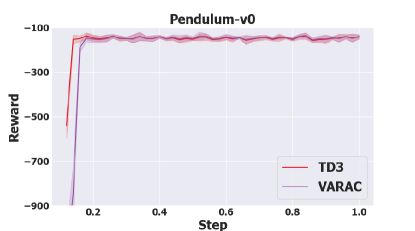
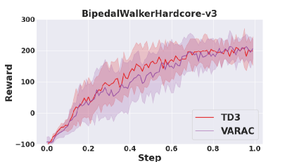
Figure 1: We present the training progress of TD3 and VARAC algorithms in the figure. In the graph, the $y$-axis represents the average reward value obtained after evaluating each checkpoint, while the $x$-axis represents the ratio of training steps to the total number of steps, indicating the extent of training progress. The curves are averaged over ten independent runs with shaded regions indicating standard deviations.

Algorithm	Pendulum-v0		BipedalWalkerHardcore-v3
	Mean	Variance	Mean	Variance
TD3	-122	6903	234	9348
VARAC	-126	4826	221	6090

Table 1: The mean and variance of the policy learned by TD3 and VARAC algorithms under two gym environments.

7 Conclusion

To conclude, to the best of our knowledge, we make the first attempt to study risk-sensitive deep reinforcement learning, where we consider the variance constrained deep reinforcement learning. We propose an efficient and theoretically sound VARAC algorithm to solve the problem. Under mild assumptions, despite the overparametrization and nonconvexity, we show that our algorithm achieves an $\mathcal{O}(1/\sqrt{K})$ convergence rate to a saddle point, and that our solution converges to a globally optimal solution at a same rate. For future work, we plan to extend the risk constraints to other coherent risk measures such as the conditional value at risk.

Appendix

Appendix A Algorithms in Section 3

We present the algorithms for solving the subproblems of policy improvement and policy evaluation in Section 3.

Algorithm 2 Update $\theta$ via SGD

1:  Require: MDP $({\mathcal{S}},\mathcal{A},{\mathcal{P}},r,\gamma)$, current energy function $f_{\theta_{k}}$, initial actor parameter $\theta_{0}$, number of iterations $T$, sample $\{(s_{t},a^{0}_{t})\}^{T}_{t=1}$

2:  Initialization: $\theta(0)\leftarrow\theta_{0}$

3:  Set stepsize $\zeta\leftarrow{T}^{-1/2}$

4:  for $t=0,\dots,T-1$ do

5:     Sample $(s,a)\leftarrow(s_{t+1},a^{0}_{t+1})$

6:     $\theta(t+1)\leftarrow\Pi_{{\mathcal{B}}(\theta_{0},R_{a})}\bigl{(}\theta(t)-\zeta\cdot\bigl{(}f_{\theta(t)}(s,a)-\tau_{k+1}\cdot(\beta_{k}^{-1}(1+2\overline{\lambda}_{k}\overline{y}_{k})Q_{q_{k}}+\beta_{k}^{-1}\overline{\lambda}_{k}W_{\omega_{k}}+\tau^{-1}_{k}f_{\theta_{k}}(s,a))\bigr{)}\cdot\nabla_{\theta}f_{\theta(t)}(s,a)\bigr{)}$

7:  end for

8:  Average over path $\overline{\theta}\leftarrow 1/T\cdot\sum^{T-1}_{t=0}\theta(t)$

9:  Output: $f_{\overline{\theta}}$

Algorithm 3 Update $q$ via TD(0)

1:  Require: MDP $({\mathcal{S}},\mathcal{A},{\mathcal{P}},r)$, initial critic parameter $q_{0}$, number of iterations $T$, sample $\{(s_{t},a_{t},s_{t}^{\prime},a_{t}^{\prime})\}^{T}_{t=1}$

2:  Initialization: $q(0)\leftarrow q_{0}$

3:  Set stepsize $\delta\leftarrow T^{-1/2}$

4:  for $t=0,\dots,T-1$ do

5:     Sample $(s,a,s^{\prime},a^{\prime})$ $\leftarrow(s_{t+1},a_{t+1},s^{\prime}_{t+1},a^{\prime}_{t+1})$

6:     $q(t+1)\leftarrow\Pi_{{\mathcal{B}}(q_{0},R_{c})}\bigl{(}q(t)-\delta\cdot\bigl{(}Q_{q(t)}(s,a)-r(s,a)+\overline{\rho}(\pi_{\theta_{k}})-Q_{q(t)}(s^{\prime},a^{\prime})\bigr{)}\cdot\nabla_{q}Q_{q(t)}(s,a)\bigr{)}$

7:  end for

8:  Average over path $\overline{q}\leftarrow 1/T\cdot\sum^{T-1}_{t=0}q(t)$

9:  Output: $Q_{\overline{q}}$

Algorithm 4 Update $\omega$ via TD(0)

1:  Require: MDP $({\mathcal{S}},\mathcal{A},{\mathcal{P}},r,\gamma)$, initial critic parameter $\omega_{0}$, number of iterations $T$, sample $\{(s_{t},a_{t},s_{t}^{\prime},a_{t}^{\prime})\}^{T}_{t=1}$

2:  Initialization: $\omega(0)\leftarrow\omega_{0}$

3:  Set stepsize $\delta\leftarrow T^{-1/2}$

4:  for $t=0,\dots,T-1$ do

5:     Sample $(s,a,s^{\prime},a^{\prime})\leftarrow(s_{t+1},a_{t+1},s^{\prime}_{t+1},a^{\prime}_{t+1})$

6:     $\omega(t+1)\leftarrow\Pi_{{\mathcal{B}}(\omega_{0},R_{b})}\bigl{(}\omega(t)-\delta\cdot\bigl{(}W_{\omega(t)}(s,a)-r(s,a)+\overline{\eta}(\pi_{\theta_{k}})-W_{\omega(t)}(s^{\prime},a^{\prime})\bigr{)}\cdot\nabla_{\omega}Q_{\omega(t)}(s,a)\bigr{)}$

7:  end for

8:  Average over path $\overline{\omega}\leftarrow 1/T\cdot\sum^{T-1}_{t=0}\omega(t)$

9:  Output: $W_{\overline{\omega}}$

Appendix B Proof of Proposition 3.1

Proof.

The subproblem of policy improvement for solving $\widehat{\pi}_{k+1}$ takes the form

$$\max_{\pi}~{}\mathbb{E}_{\nu_{k}}\bigl{[}\langle\pi(\cdot\,|\,s),(1+2\overline{\lambda}_{k}\overline{y}_{k})Q_{q_{k}}(s,a)-\overline{\lambda}_{k}W_{\omega_{k}}(s,a)\rangle-\beta_{k}\cdot{\rm KL}\bigl{(}\pi(\cdot\,|\,s)\,\|\,\pi_{\theta_{k}}(\cdot\,|\,s)\bigr{)}\bigr{]}$$

$$~{}\text{subject to }\sum_{a\in\mathcal{A}}\pi(a\,|\,s)=1,~{}~{}\text{for any}~{}s\in{\mathcal{S}}.$$

We consider the Lagrangian dual function of the above maximization problem that

$$\int_{s\in{\mathcal{S}}}\bigl{[}\langle\pi(\cdot\,|\,s),(1+2\overline{\lambda}_{k}\overline{y}_{k})Q_{q_{k}}(s,a)-\overline{\lambda}_{k}W_{\omega_{k}}(s,a)\rangle-\beta_{k}\cdot{\rm KL}\bigl{(}\pi(\cdot\,|\,s)\,\|\,\pi_{\theta_{k}}(\cdot\,|\,s)\bigr{)}\bigr{]}\nu_{k}({\mathrm{d}}s)$$

$$\qquad+\int_{s\in{\mathcal{S}}}\biggl{(}\sum_{a\in\mathcal{A}}\pi(a\,|\,s)-1\biggr{)}\lambda({\mathrm{d}}s).$$

Recall that we restrict the solution be an energy-based policy that $\pi_{\theta_{k}}\propto\exp(\tau_{k}^{-1}f_{\theta_{k}})$. Plugging $\pi_{\theta_{k}}(s,a)=\exp(\tau_{k}^{-1}f_{\theta_{k}}(s,a))/\sum_{a^{\prime}\in\mathcal{A}}\exp(\tau_{k}^{-1}f_{\theta_{k}}(s,a^{\prime}))$ into the above function and taking the derivative, we obtain the optimality condition

$$(1+2\overline{\lambda}_{k}\overline{y}_{k})Q_{q_{k}}(s,a)-\overline{\lambda}_{k}W_{\omega_{k}}(s,a)+\beta_{k}\tau_{k}^{-1}f_{\theta_{k}}(s,a)$$

$$\qquad-\beta_{k}\cdot\bigg{[}\log\biggl{(}\sum_{a^{\prime}\in\mathcal{A}}\exp\bigl{(}\tau_{k}^{-1}f_{\theta_{k}}(s,a^{\prime})\bigr{)}\biggr{)}+\log\pi(a\,|s)+1\biggr{]}+\frac{\lambda(s)}{\nu_{k}(s)}=0,$$

for any $a\in\mathcal{A}$ and $s\in{\mathcal{S}}$. Note that $\log(\sum_{a^{\prime}\in\mathcal{A}}\exp(\tau_{k}^{-1}f_{\theta_{k}}(s,a^{\prime})))$ is determined by the state $s$ only. Thus, for any $(s,a)\in{\mathcal{S}}\times\mathcal{A}$, we have

$$\widehat{\pi}_{k+1}(a\,|\,s)\propto\exp\bigl{(}\beta_{k}^{-1}(1+2\overline{\lambda}_{k}\overline{y}_{k})Q_{q_{k}}(s,a)-\beta_{k}^{-1}\overline{\lambda}_{k}W_{\omega_{k}}(s,a)+\tau_{k}^{-1}f_{\theta_{k}}(s,a)\bigr{)},$$

which completes the proof. ∎

Appendix C Proofs for Section 4.2

Proof of Lemma 4.6.

Let the local linearization of $Q_{q}$ be

$$\overline{Q}_{q}=Q_{q_{0}}+(q-q_{0})^{\top}\nabla_{q_{0}}Q_{q}.$$ (C.1)

We denote by

$$g_{t}=\bigl{(}Q_{q(t)}(s,a)-Q_{q(t)}(s^{\prime},a^{\prime})-r_{0}+\overline{\rho}(\pi_{\theta})\bigr{)}\cdot\nabla_{q}Q_{q(t)}(s,a), g_{t}^{e}=\mathbb{E}_{\pi_{\theta}}[g_{n}],$$

$$\overline{g}_{t}=\bigl{(}\overline{Q}_{q_{(}t)}(s,a)-\overline{Q}_{q(t)}(s^{\prime},a^{\prime})-r_{0}+\overline{\rho}(\pi_{\theta})\bigr{)}\cdot\nabla_{q}Q_{q_{0}}(s,a), \overline{g}_{t}^{e}=\mathbb{E}_{\pi_{\theta}}[\overline{g}_{n}],$$

$$g_{*}=\bigl{(}Q_{q_{*}}(s,a)-Q_{q_{*}}(s^{\prime},a^{\prime})-r_{0}+\overline{\rho}(\pi_{\theta})\bigr{)}\cdot\nabla_{q}Q_{q_{*}}(s,a), g_{*}^{e}=\mathbb{E}_{\pi_{\theta}}[g_{*}],$$

$$\overline{g}_{*}=\bigl{(}\overline{Q}_{q_{*}}(s,a)-\overline{Q}_{q_{*}}(s^{\prime},a^{\prime})-r_{0}+\overline{\rho}(\pi_{\theta})\bigr{)}\cdot\nabla_{q}Q_{q_{0}}(s,a), \overline{g}_{*}^{e}=\mathbb{E}_{\pi_{\theta}}[\overline{g}_{*}],$$ (C.2)

where $q_{*}$ satisfies that

$$q_{*}=\Pi_{{\mathcal{B}}(q_{0},R_{\rm c})}(q_{*}-\delta\cdot\overline{g}_{*}^{e}).$$

Here the expectation $\mathbb{E}_{\pi_{\theta}}[\cdot]$ is taken following $(s,a)\sim\rho_{\pi_{\theta}}(\cdot)$, $s^{\prime}\sim P(\cdot\,|\,s,a)$, $a^{\prime}\sim\pi_{\theta}(\cdot\,|\,s_{1})$, and $r_{0}=\mathcal{R}(s,a)$. By Algorithm 3, we have that

$$q(t+1)=\Pi_{{\mathcal{B}}(q_{0},R_{\rm c})}\big{(}q(t)-\delta\cdot g_{t}\big{)}.$$

Then, we have

$$\mathbb{E}_{\pi_{\theta}}\bigl{[}\|q(t+1)-q_{*}\|_{2}^{2}\,|\,q(t)\bigr{]}$$

$$\qquad=\mathbb{E}_{\pi_{\theta}}\bigl{[}\|\Pi_{{\mathcal{B}}(q_{0},R_{\rm c})}(q(t)-\delta\cdot g_{t})-\Pi_{{\mathcal{B}}(q_{0},R_{\rm c})}(q_{*}-\delta\cdot\overline{g}_{*}^{e})\|_{2}^{2}\,|\,q(t)\bigr{]}$$

$$\qquad\leq\mathbb{E}_{\pi_{\theta}}\bigl{[}\|(q(t)-\delta\cdot g_{t})-(q_{*}-\delta\cdot\overline{g}_{*}^{e})\|_{2}^{2}\,|\,q(t)\bigr{]}$$

$$\qquad=\|q(t)-q_{*}\|_{2}^{2}+2\delta\cdot\langle q_{*}-q(t),g_{t}^{e}-\overline{g}_{*}^{e}\rangle+\delta^{2}\cdot\mathbb{E}_{\pi_{\theta}}\bigl{[}\|g_{t}-\overline{g}_{*}^{e}\|_{2}^{2}\,|\,q(t)\bigr{]}.$$ (C.3)

We upper bound the second term on the right hand side of (C) in the sequel. By Hölder’s inequality, it holds that

$$\langle q_{*}-q(t),g_{t}^{e}-\overline{g}_{*}^{e}\rangle$$

$$\qquad=\langle q_{*}-q(t),g_{t}^{e}-\overline{g}_{t}^{e}\rangle+\langle q_{*}-q(t),\overline{g}_{t}^{e}-\overline{g}_{*}^{e}\rangle$$

$$\qquad\leq\|q_{*}-q(t)\|_{2}\cdot\|g_{t}^{e}-\overline{g}_{t}^{e}\|_{2}+\langle q_{*}-q(t),\overline{g}_{t}^{e}-\overline{g}_{*}^{e}\rangle$$

$$\qquad\leq 2R_{\rm c}\cdot\|g_{t}^{e}-\overline{g}_{t}^{e}\|_{2}+\langle q_{*}-q(t),\overline{g}_{t}^{e}-\overline{g}_{*}^{e}\rangle,$$ (C.4)

where the last inequality is obtained by the fact that $q(t),q_{*}\in{\mathcal{B}}(q_{0},R_{\rm c})$. By the definitions in (C), we further obtain

$$\langle q_{*}-q(t),\overline{g}_{t}^{e}-\overline{g}_{*}^{e}\rangle$$

$$\qquad=\mathbb{E}_{\pi_{\theta}}\bigl{[}\bigl{(}(\overline{Q}_{q(t)}(s,a)-\overline{Q}_{q_{*}}(s,a))-(\overline{Q}_{q(t)}(s^{\prime},a^{\prime})-\overline{Q}_{q_{*}}(s^{\prime},a^{\prime}))\bigr{)}\cdot\langle q_{*}-q(t),\nabla_{q}Q_{q_{0}}(s,a)\rangle\bigr{]}$$

$$\qquad=\mathbb{E}_{\pi_{\theta}}\bigl{[}\bigl{(}(\overline{Q}_{q(t)}(s,a)-\overline{Q}_{q_{*}}(s,a))-(\overline{Q}_{q(t)}(s^{\prime},a^{\prime})-\overline{Q}_{q_{*}}(s^{\prime},a^{\prime}))\bigr{)}\cdot(\overline{Q}_{q_{*}}(s,a)-\overline{Q}_{q(t)}(s,a))\bigr{]}$$

$$\qquad=\mathbb{E}_{\pi_{\theta}}\bigl{[}(\overline{Q}_{q(t)}(s,a)-\overline{Q}_{q_{*}}(s,a))\cdot(\overline{Q}_{q(t)}(s^{\prime},a^{\prime})-\overline{Q}_{q_{*}}(s^{\prime},a^{\prime}))\bigr{]}$$

$$\qquad\qquad-\mathbb{E}_{\pi_{\theta}}\bigl{[}(\overline{Q}_{q(t)}(s,a)-\overline{Q}_{q_{*}}(s,a))^{2}\bigr{]},$$ (C.5)

where the second equality is obtained by (C.1). By Cauchy-Schwartz inequality, we further have

$$\mathbb{E}_{\pi_{\theta}}\bigl{[}(\overline{Q}_{q(t)}(s,a)-\overline{Q}_{q_{*}}(s,a))\cdot(\overline{Q}_{q(t)}(s^{\prime},a^{\prime})-\overline{Q}_{q_{*}}(s^{\prime},a^{\prime}))\bigr{]}$$

$$\qquad\leq[\mathbb{E}_{\pi_{\theta}}\bigl{[}(\overline{Q}_{q(t)}(s,a)-\overline{Q}_{q_{*}}(s,a))^{2}\bigr{]}]^{\frac{1}{2}}\cdot[\mathbb{E}_{\pi_{\theta}}\bigl{[}(\overline{Q}_{q(t)}(s^{\prime},a^{\prime})-\overline{Q}_{q_{*}}(s^{\prime},a^{\prime}))^{2}\bigr{]}]^{\frac{1}{2}}$$

$$\qquad\leq\beta_{\pi_{\theta}}\cdot\mathbb{E}_{\pi_{\theta}}\bigl{[}(\overline{Q}_{q(t)}(s,a)-\overline{Q}_{q_{*}}(s,a))^{2}\bigr{]},$$ (C.6)

where the last inequality holds by Assumption 4.3. Combining (C), (C) and (C), we have

$$\langle q_{*}-q(t),\overline{g}_{t}^{e}-\overline{g}_{*}^{e}\rangle\leq 2R_{\rm c}\cdot\|g_{t}^{e}-\overline{g}_{t}^{e}\|_{2}-(1-\beta_{\pi_{\theta}})\mathbb{E}_{\rho_{\pi_{\theta}}}\bigl{[}(\overline{Q}_{q(t)}-\overline{Q}_{q_{*}})^{2}\bigr{]}.$$

The remaining proof follows Fu et al. (2020). ∎

Appendix D Proofs for Section 4.3

Proof of Lemma 4.8.

We first have by (4.2), and recall that we restrict $\pi_{\theta_{k}}\propto\exp(\tau_{k}^{-1}f_{\theta_{k}})$,

$$\pi_{k+1}(a\,|\,s)=\exp\bigl{(}\beta_{k}^{-1}(1+2\overline{\lambda}_{k}\overline{y}_{k})Q^{\pi_{\theta_{k}}}(s,a)-\beta_{k}^{-1}\overline{\lambda}_{k}W^{\pi_{\theta_{k}}}(s,a)+\tau_{k}^{-1}f_{\theta_{k}}(s,a)\bigr{)}/Z_{k+1}(s),$$

and

$$\pi_{\theta_{k+1}}(a\,|\,s)=\exp\bigl{(}\tau_{k+1}^{-1}f_{\theta_{k+1}}(s,a)\bigr{)}/Z_{\theta_{k+1}}(s),$$

where $Z_{k+1}(s),Z_{\theta_{k+1}}(s)\in\mathbb{R}$ are normalization factors, which are defined as

$$Z_{k+1}(s) =\sum_{a^{\prime}\in\mathcal{A}}\exp\bigl{(}\beta_{k}^{-1}(1+2\overline{\lambda}_{k}\overline{y}_{k})Q^{\pi_{\theta_{k}}}(s,a^{\prime})-\beta_{k}^{-1}\overline{\lambda}_{k}W^{\pi_{\theta_{k}}}(s,a^{\prime})+\tau_{k}^{-1}f_{\theta_{k}}(s,a^{\prime})\bigr{)},$$

$$Z_{\theta_{k+1}}(s) =\sum_{a^{\prime}\in\mathcal{A}}\exp\bigl{(}\tau_{k+1}^{-1}f_{\theta_{k+1}}(s,a^{\prime})\bigr{)},$$ (D.1)

respectively. Then, we reformulate the inner product in (4.7) as

$$\langle\log\pi_{\theta_{k+1}}(\cdot\,|\,s)-\log\pi_{k+1}(\cdot\,|\,s),\pi^{*}(\cdot\,|\,s)-\pi_{\theta_{k}}(\cdot\,|\,s)\rangle$$

$$\qquad=\big{\langle}\tau_{k+1}^{-1}f_{\theta_{k+1}}(s,\cdot)-\big{(}\beta_{k}^{-1}(1+2\overline{\lambda}_{k}\overline{y}_{k})Q^{\pi_{\theta_{k}}}(s,\cdot)-\beta_{k}^{-1}\overline{\lambda}_{k}W^{\pi_{\theta_{k}}}(s,\cdot)$$

$$\qquad\qquad+\tau_{k}^{-1}f_{\theta_{k}}(s,\cdot)\big{)},\pi^{*}(\cdot\,|\,s)-\pi_{\theta_{k}}(\cdot\,|\,s)\big{\rangle},$$ (D.2)

where we use the fact that

$$\langle\log Z_{k+1}(s)-\log Z_{\theta_{k+1}}(s),\pi^{*}(\cdot\,|\,s)-\pi_{\theta_{k}}(\cdot\,|\,s)\rangle$$

$$\qquad=(\log Z_{k+1}(s)-\log Z_{\theta_{k+1}}(s))\sum_{a^{\prime}\in\mathcal{A}}\bigl{(}\pi^{*}(a^{\prime}\,|\,s)-\pi_{\theta_{k}}(a^{\prime}\,|\,s)\bigr{)}=0.$$

Thus, it remains to upper bound the right-hand side of (D). We first decompose it to three terms, namely the error from learning the Q-function and the error from fitting the improved policy, that is,

$$\langle\tau_{k+1}^{-1}f_{\theta_{k+1}}(s,\cdot)-(\beta_{k}^{-1}(1+2\overline{\lambda}_{k}\overline{y}_{k})Q^{\pi_{\theta_{k}}}(s,\cdot)-\beta_{k}^{-1}\overline{\lambda}_{k}W^{\pi_{\theta_{k}}}(s,\cdot)+\tau_{k}^{-1}f_{\theta_{k}}(s,\cdot)),\pi^{*}(\cdot\,|\,s)-\pi_{\theta_{k}}(\cdot\,|\,s)\rangle$$

$$\qquad=\underbrace{\langle\tau_{k+1}^{-1}f_{\theta_{k+1}}(s,\cdot)-(\beta_{k}^{-1}(1+2\overline{\lambda}_{k}\overline{y}_{k})Q_{q_{k}}(s,\cdot)-\beta_{k}^{-1}\overline{\lambda}_{k}W_{\omega_{k}}(s,\cdot)+\tau_{k}^{-1}f_{\theta_{k}}(s,\cdot)),\pi^{*}(\cdot\,|\,s)-\pi_{\theta_{k}}(\cdot\,|\,s)\rangle}_{\displaystyle{\rm(i)}}$$

$$\qquad\qquad+\underbrace{(1+2\overline{\lambda}_{k}\overline{y}_{k})\cdot\langle\beta_{k}^{-1}Q_{q_{k}}(s,\cdot)-\beta_{k}^{-1}Q^{\pi_{\theta_{k}}}(s,\cdot),\pi^{*}(\cdot\,|\,s)-\pi_{\theta_{k}}(\cdot\,|\,s)\rangle}_{\displaystyle{\rm(ii)}}$$

$$\qquad\qquad+\underbrace{\overline{\lambda}_{k}\cdot\langle\beta_{k}^{-1}W^{\pi_{\theta_{k}}}(s,\cdot)-\beta_{k}^{-1}W_{\omega_{k}}(s,\cdot),\pi^{*}(\cdot\,|\,s)-\pi_{\theta_{k}}(\cdot\,|\,s)\rangle}_{\displaystyle{\rm(iii)}}.$$ (D.3)

Upper Bounding (i): We have

$$\langle\tau_{k+1}^{-1}f_{\theta_{k+1}}(s,\cdot)-(\beta_{k}^{-1}(1+2\overline{\lambda}_{k}\overline{y}_{k})Q_{q_{k}}(s,\cdot)-\beta_{k}^{-1}\overline{\lambda}_{k}W_{\omega_{k}}(s,\cdot)+\tau_{k}^{-1}f_{\theta_{k}}(s,\cdot)),\pi^{*}(\cdot\,|\,s)-\pi_{\theta_{k}}(\cdot\,|\,s)\rangle$$

$$\qquad=\biggl{\langle}\tau_{k+1}^{-1}f_{\theta_{k+1}}(s,\cdot)-(\beta_{k}^{-1}(1+2\overline{\lambda}_{k}\overline{y}_{k})Q_{q_{k}}(s,\cdot)-\beta_{k}^{-1}\overline{\lambda}_{k}W_{\omega_{k}}(s,\cdot)$$

$$\qquad\qquad+\tau_{k}^{-1}f_{\theta_{k}}(s,\cdot)),\pi_{0}(\cdot\,|\,s)\cdot\biggl{(}\frac{\pi^{*}(\cdot\,|\,s)}{\pi_{0}(\cdot\,|\,s)}-\frac{\pi_{\theta_{k}}(\cdot\,|\,s)}{\pi_{0}(\cdot\,|\,s)}\biggr{)}\biggr{\rangle}.$$ (D.4)

Taking expectation with respect to $s\sim\nu^{*}$ on the both sides of (D), we obtain

$$\bigl{|}\mathbb{E}_{\nu^{*}}[\langle\tau_{k+1}^{-1}f_{\theta_{k+1}}(s,\cdot)-(\beta_{k}^{-1}(1+2\overline{\lambda}_{k}\overline{y}_{k})Q_{q_{k}}(s,\cdot)-\beta_{k}^{-1}\overline{\lambda}_{k}W_{\omega_{k}}(s,\cdot)+\tau_{k}^{-1}f_{\theta_{k}}(s,\cdot)),\pi^{*}(\cdot\,|\,s)-\pi_{\theta_{k}}(\cdot\,|\,s)\rangle]\bigr{|}$$

$$\qquad=\biggl{|}\int_{\mathcal{S}}\biggl{\langle}\tau_{k+1}^{-1}f_{\theta_{k+1}}(s,\cdot)-(\beta_{k}^{-1}(1+2\overline{\lambda}_{k}\overline{y}_{k})Q_{q_{k}}(s,\cdot)-\beta_{k}^{-1}\overline{\lambda}_{k}W_{\omega_{k}}(s,\cdot)+\tau_{k}^{-1}f_{\theta_{k}}(s,\cdot)),$$

$$\qquad\qquad\pi_{0}(\cdot\,|\,s)\cdot\biggr{(}\frac{\pi^{*}(\cdot\,|\,s)}{\pi_{0}(\cdot\,|\,s)}-\frac{\pi_{\theta_{k}}(\cdot\,|\,s)}{\pi_{0}(\cdot\,|\,s)}\biggl{)}\biggr{\rangle}\cdot\nu^{*}(s){\mathrm{d}}s\biggr{|}$$

$$\qquad=\biggl{|}\int_{{\mathcal{S}}\times\mathcal{A}}\bigl{(}\tau_{k+1}^{-1}f_{\theta_{k+1}}(s,a)-(\beta_{k}^{-1}(1+2\overline{\lambda}_{k}\overline{y}_{k})Q_{q_{k}}(s,a)-\beta_{k}^{-1}\overline{\lambda}_{k}W_{\omega_{k}}(s,a)+\tau_{k}^{-1}f_{\theta_{k}}(s,a))\bigr{)}$$

$$\qquad\qquad\cdot\biggl{(}\frac{\pi^{*}(\cdot\,|\,s)}{\pi_{0}(\cdot\,|\,s)}-\frac{\pi_{\theta_{k}}(\cdot\,|\,s)}{\pi_{0}(\cdot\,|\,s)}\biggr{)}{\mathrm{d}}{\sigma}_{k}(s,a)\biggr{|}.$$

By Cauchy-Schwarz inequality, we further have

$$\bigl{|}\mathbb{E}_{\nu^{*}}[\langle\tau_{k+1}^{-1}f_{\theta_{k+1}}(s,\cdot)-(\beta_{k}^{-1}(1+2\overline{\lambda}_{k}\overline{y}_{k})Q_{q_{k}}(s,\cdot)-\beta_{k}^{-1}\overline{\lambda}_{k}W_{\omega_{k}}(s,\cdot)+\tau_{k}^{-1}f_{\theta_{k}}(s,\cdot)),\pi^{*}(\cdot\,|\,s)-\pi_{\theta_{k}}(\cdot\,|\,s)\rangle]\bigr{|}$$

$$\qquad\leq\mathbb{E}_{{\sigma}_{k}}[\bigl{(}\tau_{k+1}^{-1}f_{\theta_{k+1}}(s,a)-(\beta_{k}^{-1}(1+2\overline{\lambda}_{k}\overline{y}_{k})Q_{q_{k}}(s,a)-\beta_{k}^{-1}\overline{\lambda}_{k}W_{\omega_{k}}(s,a)+\tau_{k}^{-1}f_{\theta_{k}}(s,a))\bigr{)}^{2}]^{1/2}$$

$$\qquad\qquad\cdot\mathbb{E}_{{\sigma}_{k}}\biggl{[}\biggl{|}\biggl{(}\frac{{\mathrm{d}}\pi^{*}}{{\mathrm{d}}\pi_{0}}-\frac{{\mathrm{d}}\pi_{\theta_{k}}}{{\mathrm{d}}\pi_{0}}\biggr{)}\biggr{|}^{2}\biggr{]}^{1/2}$$

$$\qquad\leq\tau_{k+1}^{-1}\epsilon_{k+1}\cdot\phi^{*}_{k},$$ (D.5)

where in the last inequality holds by (4.4) and the definition of $\phi^{*}_{k}$ in (4.3).

Upper Bounding (ii): By the updating rule of $\lambda$ and $y$, we have $|\overline{\lambda}_{k}|\leq N$ and $|\overline{y}_{k}|\leq M$. Thus, we have

$$|(1+2\overline{\lambda}_{k}\overline{y}_{k})\cdot\mathbb{E}_{\nu^{*}}[\langle\beta_{k}^{-1}Q_{q_{k}}(s,\cdot)-\beta_{k}^{-1}Q^{\pi_{\theta_{k}}}(s,\cdot),\pi^{*}(\cdot\,|\,s)-\pi_{\theta_{k}}(\cdot\,|\,s)\rangle]|$$

$$\qquad\leq(1+2MN)\cdot|\mathbb{E}_{\nu^{*}}[\langle\beta_{k}^{-1}Q_{q_{k}}(s,\cdot)-\beta_{k}^{-1}Q^{\pi_{\theta_{k}}}(s,\cdot),\pi^{*}(\cdot\,|\,s)-\pi_{\theta_{k}}(\cdot\,|\,s)\rangle]|$$

$$\qquad=(1+2MN)\cdot\biggl{|}\int_{{\mathcal{S}}\times\mathcal{A}}(\beta_{k}^{-1}Q_{q_{k}}(s,a)-\beta_{k}^{-1}Q^{\pi_{\theta_{k}}}(s,a))\cdot\biggl{(}\frac{\pi^{*}(a\,|\,s)}{\pi_{\theta_{k}}(a\,|\,s)}-\frac{\pi_{\theta_{k}}(a\,|\,s)}{\pi_{\theta_{k}}(a\,|\,s)}\biggr{)}\cdot\frac{\nu^{*}(s)}{\nu_{k}(s)}{\mathrm{d}}\sigma_{k}(s,a)\biggr{|}.$$

By Cauchy-Schwartz inequality, we further have

$$|(1+2\overline{\lambda}_{k}\overline{y}_{k})\cdot\mathbb{E}_{\nu^{*}}[\langle\beta_{k}^{-1}Q_{q_{k}}(s,\cdot)-\beta_{k}^{-1}Q^{\pi_{\theta_{k}}}(s,\cdot),\pi^{*}(\cdot\,|\,s)-\pi_{\theta_{k}}(\cdot\,|\,s)\rangle]|$$

$$\qquad\leq(1+2MN)\cdot\mathbb{E}_{\sigma_{k}}[(\beta_{k}^{-1}Q_{q_{k}}(s,a)-\beta_{k}^{-1}Q^{\pi_{\theta_{k}}}(s,a))^{2}]^{1/2}\cdot\mathbb{E}_{\sigma_{k}}\biggl{[}\biggl{|}\frac{{\mathrm{d}}\sigma^{*}}{{\mathrm{d}}\sigma_{k}}-\frac{{\mathrm{d}}\nu^{*}}{{\mathrm{d}}\nu_{k}}\biggr{|}^{2}\biggr{]}^{1/2}$$

$$\qquad\leq(1+2MN)\cdot\beta_{k}^{-1}\epsilon_{k}^{\prime}\cdot\psi^{*}_{k},$$ (D.6)

where the last inequality holds by the error bound (4.5) and the definition of $\psi^{*}_{k}$ (4.3).

Upper Bounding (iii): By the updating rule of $\lambda$, we have $|\overline{\lambda}_{k}|\leq N$. Thus, we have

$$|\overline{\lambda}_{k}\cdot\mathbb{E}_{\nu^{*}}[\langle\beta_{k}^{-1}W^{\pi_{\theta_{k}}}(s,\cdot)-\beta_{k}^{-1}W_{\omega_{k}}(s,\cdot),\pi^{*}(\cdot\,|\,s)-\pi_{\theta_{k}}(\cdot\,|\,s)\rangle]|$$

$$\qquad\leq N\cdot|\mathbb{E}_{\nu^{*}}[\langle\beta_{k}^{-1}W^{\pi_{\theta_{k}}}(s,\cdot)-\beta_{k}^{-1}W_{\omega_{k}}(s,\cdot),\pi^{*}(\cdot\,|\,s)-\pi_{\theta_{k}}(\cdot\,|\,s)\rangle]|$$

$$\qquad=N\cdot\biggl{|}\int_{{\mathcal{S}}\times\mathcal{A}}(\beta_{k}^{-1}W^{\pi_{\theta_{k}}}(s,a)-\beta_{k}^{-1}W_{\omega_{k}}(s,a))\cdot\biggl{(}\frac{\pi^{*}(a\,|\,s)}{\pi_{\theta_{k}}(a\,|\,s)}-\frac{\pi_{\theta_{k}}(a\,|\,s)}{\pi_{\theta_{k}}(a\,|\,s)}\biggr{)}\cdot\frac{\nu^{*}(s)}{\nu_{k}(s)}{\mathrm{d}}\sigma_{k}(s,a)\biggr{|}.$$

By Cauchy-Schwartz inequality, we further have

$$|\overline{\lambda}_{k}\cdot\mathbb{E}_{\nu^{*}}[\langle\beta_{k}^{-1}W^{\pi_{\theta_{k}}}(s,\cdot)-\beta_{k}^{-1}W_{\omega_{k}}(s,\cdot),\pi^{*}(\cdot\,|\,s)-\pi_{\theta_{k}}(\cdot\,|\,s)\rangle]|$$

$$\qquad\leq N\cdot\mathbb{E}_{\sigma_{k}}[(\beta_{k}^{-1}W^{\pi_{\theta_{k}}}(s,a)-\beta_{k}^{-1}W_{\omega_{k}}(s,a))^{2}]^{1/2}\cdot\mathbb{E}_{\sigma_{k}}\biggl{[}\biggl{|}\frac{{\mathrm{d}}\sigma^{*}}{{\mathrm{d}}\sigma_{k}}-\frac{{\mathrm{d}}\nu^{*}}{{\mathrm{d}}\nu_{k}}\biggr{|}^{2}\biggr{]}^{1/2}$$

$$\qquad\leq N\cdot\beta_{k}^{-1}\epsilon_{k}^{\prime\prime}\cdot\psi^{*}_{k},$$ (D.7)

Finally, combining (D), (D), (D), (D) and (D), we have

$$|\mathbb{E}_{\nu^{*}}[\langle\log\pi_{\theta_{k+1}}(\cdot\,|\,s)-\log\pi_{k+1}(\cdot\,|\,s),\pi^{*}(\cdot\,|\,s)-\pi_{\theta_{k}}(\cdot\,|\,s)\rangle]|$$

$$\qquad\leq\tau_{k+1}^{-1}\epsilon_{k+1}\cdot\phi^{*}_{k}+(1+2MN)\cdot\beta_{k}^{-1}\epsilon_{k}^{\prime}\cdot\psi^{*}_{k}+N\cdot\beta_{k}^{-1}\epsilon_{k}^{\prime\prime}\cdot\psi^{*}_{k},$$

which concludes the proof. ∎

Proof of Lemma 4.9.

By the triangle inequality, we have

$$\|\tau_{k+1}^{-1}f_{\theta_{k+1}}(s,\cdot)-\tau_{k}^{-1}f_{\theta_{k}}(s,\cdot)\|_{\infty}^{2}$$

$$\qquad\leq 2\|\tau_{k+1}^{-1}f_{\theta_{k+1}}(s,\cdot)-\tau_{k}^{-1}f_{\theta_{k}}(s,\cdot)-\beta_{k}^{-1}(1+2\overline{\lambda}_{k}\overline{y}_{k})Q_{q_{k}}(s,\cdot)+\beta^{-1}\overline{\lambda}_{k}W_{\omega_{k}}\|_{\infty}^{2}$$

$$\qquad\qquad+2\|\beta_{k}^{-1}(1+2\overline{\lambda}_{k}\overline{y}_{k})Q_{q_{k}}(s,\cdot)-\beta^{-1}\overline{\lambda}_{k}W_{\omega_{k}}\|_{\infty}^{2}$$

$$\qquad\leq 2\|\tau_{k+1}^{-1}f_{\theta_{k+1}}(s,\cdot)-\tau_{k}^{-1}f_{\theta_{k}}(s,\cdot)-\beta_{k}^{-1}(1+2\overline{\lambda}_{k}\overline{y}_{k})Q_{q_{k}}(s,\cdot)+\beta^{-1}\overline{\lambda}_{k}W_{\omega_{k}}\|_{\infty}^{2}$$

$$\qquad\qquad+4\|\beta_{k}^{-1}(1+2\overline{\lambda}_{k}\overline{y}_{k})Q_{q_{k}}(s,\cdot)\|_{\infty}^{2}+4\|\beta^{-1}\overline{\lambda}_{k}W_{\omega_{k}}\|_{\infty}^{2}.$$ (D.8)

For the first term on the right-hand side of (D), by Lemma 4.8, we have

$$\mathbb{E}_{\nu^{*}}[\|\tau_{k+1}^{-1}f_{\theta_{k+1}}(s,\cdot)-\tau_{k}^{-1}f_{\theta_{k}}(s,\cdot)-\beta_{k}^{-1}(1+2\overline{\lambda}_{k}\overline{y}_{k})Q_{q_{k}}(s,\cdot)+\beta^{-1}\overline{\lambda}_{k}W_{\omega_{k}}\|_{\infty}^{2}]\leq|\mathcal{A}|\cdot\tau_{k+1}^{-2}\epsilon_{k+1}^{2}.$$ (D.9)

For the second term on the right-hand side of (D), we have

$$\mathbb{E}_{\nu^{*}}[\|\beta_{k}^{-1}(1+2\overline{\lambda}_{k}\overline{y}_{k})Q_{q_{k}}(s,\cdot)\|_{\infty}^{2}]\leq\beta_{k}^{-2}\cdot(1+2MN)^{2}\cdot\mathbb{E}_{\nu^{*}}\Bigl{[}\max_{a\in\mathcal{A}}2(Q_{q_{0}}(s,a))^{2}+2R_{\rm c}^{2}\Bigr{]},$$ (D.10)

where we use the $1$-Lipschitz continuity of $Q_{\omega}$ in $\omega$ and the constraint $\|\omega_{k}-\omega_{0}\|_{2}\leq R_{\omega}$. For the third term on the right-hand side of (D), we have

$$\mathbb{E}_{\nu^{*}}[\|\beta^{-1}\overline{\lambda}_{k}W_{\omega_{k}}\|_{\infty}^{2}]\leq\beta_{k}^{-2}\cdot N^{2}\cdot\mathbb{E}_{\nu^{*}}\Bigl{[}\max_{a\in\mathcal{A}}2(W_{\omega_{0}}(s,a))^{2}+2R_{\rm b}^{2}\Bigr{]}.$$ (D.11)

Then, taking expectation with respect to $s\sim\nu^{*}$ on both sides of (D) and plugging (D.9), (D.10) and (D.11) in, the result holds as desired. ∎

Appendix E Proofs of Section 4.4

Proof of Lemma 4.11.

By the definition of $\rho(\pi)$ in (2.1), we have

$$\rho(\pi^{*})-\rho(\pi)=\mathbb{E}_{\nu^{*}\pi^{*}}[r(s,a)]-\rho(\pi)=\mathbb{E}_{\nu^{*}\pi^{*}}[r(s,a)-\rho(\pi)].$$ (E.1)

By the Bellman equation that $Q^{\pi}(s,a)=r(s,a)-\rho(\pi)+V^{\pi}(s^{\prime})$, we have

$$\mathbb{E}_{\nu^{*}\pi^{*}}[r(s,a)-\rho(\pi)]=\mathbb{E}_{\nu^{*}\pi^{*}}[Q^{\pi}(s,a)-V^{\pi}(s^{\prime})]=\mathbb{E}_{\nu^{*}\pi^{*}}[Q^{\pi}(s,a)-V^{\pi}(s)],$$ (E.2)

where the last equality follows from $({\mathcal{P}}^{\pi^{*}})^{t}\nu^{*}=\nu^{*}$. Finally, note that for any given $s\in{\mathcal{S}}$,

$$\mathbb{E}_{\pi^{*}}[Q^{\pi}(s,a)-V^{\pi}(s)] =\langle Q^{\pi}(s,\cdot),\pi^{*}(\cdot\,|\,s)\rangle-\langle Q^{\pi}(s,\cdot),\pi(\cdot\,|\,s)\rangle$$

$$=\langle Q^{\pi}(s,\cdot),\pi^{*}(\cdot\,|\,s)-\pi(\cdot\,|\,s)\rangle.$$ (E.3)

Plugging (E.2) and (E) into (E.1), we obtain

$$\rho(\pi^{*})-\rho(\pi)=\mathbb{E}_{\nu^{*}}[\langle Q^{\pi}(s,\cdot),\pi^{*}(\cdot\,|\,s)-\pi(\cdot\,|\,s)\rangle].$$ (E.4)

Similarly, by the definition of $\eta(\pi)$ in (2.4), we obtain

$$\eta(\pi^{*})-\eta(\pi)=\mathbb{E}_{\nu^{*}\pi^{*}}[r(s,a)^{2}]-\eta(\pi)=\mathbb{E}_{\nu^{*}\pi^{*}}[r(s,a)^{2}-\eta(\pi)].$$ (E.5)

By the equation $r(s,a)^{2}-\eta(\pi)=W^{\pi}(s,a)-U^{\pi}(s^{\prime})$, we further have

$$\mathbb{E}_{\nu^{*}\pi^{*}}[r(s,a)^{2}-\eta(\pi)]=\mathbb{E}_{\nu^{*}\pi^{*}}[W^{\pi}(s,a)-U^{\pi}(s^{\prime})]=\mathbb{E}_{\nu^{*}\pi^{*}}[W^{\pi}(s,a)-U^{\pi}(s)],$$ (E.6)

where the last equality follows from $({\mathcal{P}}^{\pi^{*}})^{t}\nu^{*}=\nu^{*}$. In addition, note that for any given $s\in{\mathcal{S}}$,

$$\mathbb{E}_{\nu^{*}\pi^{*}}[W^{\pi}(s,a)-U^{\pi}(s)] =\langle W^{\pi}(s,\cdot),\pi^{*}(\cdot\,|\,s)\rangle-\langle W^{\pi}(s,\cdot),\pi(\cdot\,|\,s)\rangle$$

$$=\mathbb{E}_{\nu^{*}}[\langle W^{\pi}(s,\cdot),\pi^{*}(\cdot\,|\,s)-\pi(\cdot\,|\,s)\rangle].$$ (E.7)

Plugging (E.6) and (E) into (E.5), we have

$$\eta(\pi^{*})-\eta(\pi)=\mathbb{E}_{\nu^{*}}[\langle W^{\pi}(s,\cdot),\pi^{*}(\cdot\,|\,s)-\pi(\cdot\,|\,s)\rangle].$$ (E.8)

Combining (E.4) and (E.8), and by the definition of ${\mathcal{L}}(\pi)$ in (3.3), we obtain

$${\mathcal{L}}(\lambda,\pi^{*},y)-{\mathcal{L}}(\lambda,\pi,y) =(1+2\lambda y)(\rho(\pi^{*})-\rho(\pi))-\lambda(\eta(\pi^{*})-\eta(\pi))$$

$$=\mathbb{E}_{\nu^{*}}[\langle(1+2\lambda y)Q^{\pi}(s,\cdot)-\lambda W^{\pi}(s,\cdot),\pi^{*}(\cdot\,|\,s)-\pi(\cdot\,|\,s)\rangle],$$

which completes the proof. ∎

Proof of Lemma 4.13.

First, we have

$${\rm KL}\bigl{(}\pi^{*}(\cdot\,|\,s)\,\|\,\pi_{\theta_{k}}(\cdot\,|\,s)\bigr{)}-{\rm KL}\bigl{(}\pi^{*}(\cdot\,|\,s)\,\|\,\pi_{\theta_{k+1}}(\cdot\,|\,s)\bigr{)}$$

$$\qquad=\langle\log(\pi_{\theta_{k+1}}(\cdot\,|\,s)/\pi_{\theta_{k}}(\cdot\,|\,s)),\pi^{*}(\cdot\,|\,s)\rangle$$

$$\qquad=\langle\log(\pi_{\theta_{k+1}}(\cdot\,|\,s)/\pi_{\theta_{k}}(\cdot\,|\,s)),\pi^{*}(\cdot\,|\,s)-\pi_{\theta_{k+1}}(\cdot\,|\,s)\rangle+{\rm KL}\bigl{(}\pi_{\theta_{k+1}}(\cdot\,|\,s)\,\|\,\pi_{\theta_{k}}(\cdot\,|\,s)\bigr{)}$$

$$\qquad=\langle\log(\pi_{\theta_{k+1}}(\cdot\,|\,s)/\pi_{\theta_{k}}(\cdot\,|\,s))-\beta_{k}^{-1}(1+\overline{\lambda}_{k}\overline{y}_{k})Q^{\pi_{\theta_{k}}}(s,\cdot)+\beta_{k}^{-1}\overline{\lambda}_{k}W^{\pi_{\theta_{k}}}(s,\cdot),\pi^{*}(\cdot\,|\,s)-\pi_{\theta_{k}}(\cdot\,|\,s)\rangle$$

$$\qquad\qquad+\beta_{k}^{-1}\cdot\langle(1+\overline{\lambda}_{k}\overline{y}_{k})Q^{\pi_{\theta_{k}}}(s,\cdot)-\overline{\lambda}_{k}W^{\pi_{\theta_{k}}}(s,\cdot),\pi^{*}(\cdot\,|\,s)-\pi_{\theta_{k}}(\cdot\,|\,s)\rangle+{\rm KL}\bigl{(}\pi_{\theta_{k+1}}(\cdot\,|\,s)\,\|\,\pi_{\theta_{k}}(\cdot\,|\,s)\bigr{)}$$

$$\qquad\qquad+\langle\log(\pi_{\theta_{k+1}}(\cdot\,|\,s)/\pi_{\theta_{k}}(\cdot\,|\,s)),\pi_{\theta_{k}}(\cdot\,|\,s)-\pi_{\theta_{k+1}}(\cdot\,|\,s)\rangle.$$ (E.9)

Recall that $\pi_{k+1}\propto\exp(\tau_{k}^{-1}f_{\theta_{k}}+\beta_{k}^{-1}(1+\overline{\lambda}_{k}\overline{y}_{k})Q^{\pi_{\theta_{k}}}-\beta_{k}^{-1}\overline{\lambda}_{k}W^{\pi_{\theta_{k}}})$ and $Z_{k+1}(s)$, and $Z_{\theta_{k}}(s)$ are defined in (D). Also recall that we have $\langle\log Z_{\theta_{k}}(s),\pi(\cdot\,|\,s)-\pi^{\prime}(\cdot\,|\,s)\rangle=\langle\log Z_{k}(s),\pi(\cdot\,|\,s)-\pi^{\prime}(\cdot\,|\,s)\rangle=0$ for all $k$, $\pi$, and $\pi^{\prime}$, which implies that, on the right-hand-side of (E),

$$\langle\log\pi_{\theta_{k}}(\cdot\,|\,s)+\beta_{k}^{-1}(1+\overline{\lambda}_{k}\overline{y}_{k})Q^{\pi_{\theta_{k}}}(s,\cdot)-\beta_{k}^{-1}\overline{\lambda}_{k}W^{\pi_{\theta_{k}}}(s,\cdot),\pi^{*}(\cdot\,|\,s)-\pi_{\theta_{k}}(\cdot\,|\,s)\rangle$$

$$\qquad=\langle\tau_{k}^{-1}f_{\theta_{k}}(s,\cdot)+\beta_{k}^{-1}(1+\overline{\lambda}_{k}\overline{y}_{k})Q^{\pi_{\theta_{k}}}(s,\cdot)-\beta_{k}^{-1}\overline{\lambda}_{k}W^{\pi_{\theta_{k}}}(s,\cdot),\pi^{*}(\cdot\,|\,s)-\pi_{\theta_{k}}(\cdot\,|\,s)\rangle$$

$$\qquad\qquad-\langle\log Z_{\theta_{k}}(s),\pi^{*}(\cdot\,|\,s)-\pi_{\theta_{k}}(\cdot\,|\,s)\rangle$$

$$\qquad=\langle\tau_{k}^{-1}f_{\theta_{k}}(s,\cdot)+\beta_{k}^{-1}(1+\overline{\lambda}_{k}\overline{y}_{k})Q^{\pi_{\theta_{k}}}(s,\cdot)-\beta_{k}^{-1}\overline{\lambda}_{k}W^{\pi_{\theta_{k}}}(s,\cdot),\pi^{*}(\cdot\,|\,s)-\pi_{\theta_{k}}(\cdot\,|\,s)\rangle$$

$$\qquad\qquad-\langle\log Z_{k+1}(s),\pi^{*}(\cdot\,|\,s)-\pi_{\theta_{k}}(\cdot\,|\,s)\rangle$$

$$\qquad=\langle\log\pi_{k+1}(\cdot\,|\,s),\pi^{*}(\cdot\,|\,s)-\pi_{\theta_{k}}(\cdot\,|\,s)\rangle,$$ (E.10)

and

$$\langle\log(\pi_{\theta_{k+1}}(\cdot\,|\,s)/\pi_{\theta_{k}}(\cdot\,|\,s)),\pi_{\theta_{k}}(\cdot\,|\,s)-\pi_{\theta_{k+1}}(\cdot\,|\,s)\rangle$$

$$\qquad=\langle\tau_{k+1}^{-1}f_{\theta_{k+1}}(s,\cdot)-\tau_{k}^{-1}f_{\theta_{k}}(s,\cdot),\pi_{\theta_{k}}(\cdot\,|\,s)-\pi_{\theta_{k+1}}(\cdot\,|\,s)\rangle$$

$$\qquad\qquad-\langle\log Z_{\theta_{k+1}}(s),\pi_{\theta_{k}}(\cdot\,|\,s)-\pi_{\theta_{k+1}}(\cdot\,|\,s)\rangle+\langle\log Z_{\theta_{k}}(s),\pi_{\theta_{k}}(\cdot\,|\,s)-\pi_{\theta_{k+1}}(\cdot\,|\,s)\rangle$$

$$\qquad=\langle\tau_{k+1}^{-1}f_{\theta_{k+1}}(s,\cdot)-\tau_{k}^{-1}f_{\theta_{k}}(s,\cdot),\pi_{\theta_{k}}(\cdot\,|\,s)-\pi_{\theta_{k+1}}(\cdot\,|\,s)\rangle.$$ (E.11)

Plugging (E) and (E) into (E), we obtain

$${\rm KL}\bigl{(}\pi^{*}(\cdot\,|\,s)\,\|\,\pi_{\theta_{k}}(\cdot\,|\,s)\bigr{)}-{\rm KL}\bigl{(}\pi^{*}(\cdot\,|\,s)\,\|\,\pi_{\theta_{k+1}}(\cdot\,|\,s)\bigr{)}$$ (E.12)

$$\qquad=\langle\log(\pi_{\theta_{k+1}}(\cdot\,|\,s)/\pi_{k+1}(\cdot\,|\,s)),\pi^{*}(\cdot\,|\,s)-\pi_{\theta_{k}}(\cdot\,|\,s)\rangle$$

$$\qquad\qquad+\beta_{k}^{-1}\cdot\langle(1+2\overline{y}_{k}\overline{\lambda}_{k})Q^{\pi_{\theta_{k}}}(s,\cdot)-\overline{\lambda}_{k}W^{\pi_{\theta_{k}}}(s,\cdot),\pi^{*}(\cdot\,|\,s)-\pi_{\theta_{k}}(\cdot\,|\,s)\rangle$$

$$\qquad\qquad+\langle\tau_{k+1}^{-1}f_{\theta_{k+1}}(s,\cdot)-\tau_{k}^{-1}f_{\theta_{k}}(s,\cdot),\pi_{\theta_{k}}(\cdot\,|\,s)-\pi_{\theta_{k+1}}(\cdot\,|\,s)\rangle+{\rm KL}\bigl{(}\pi_{\theta_{k+1}}(\cdot\,|\,s)\,\|\,\pi_{\theta_{k}}(\cdot\,|\,s)\bigr{)}$$

$$\qquad=\langle\log(\pi_{\theta_{k+1}}(\cdot\,|\,s)/\pi_{k+1}(\cdot\,|\,s)),\pi^{*}(\cdot\,|\,s)-\pi_{\theta_{k}}(\cdot\,|\,s)\rangle$$

$$\qquad\qquad+\beta_{k}^{-1}\cdot\langle(1+2y^{*}\overline{\lambda}_{k})Q^{\pi_{\theta_{k}}}(s,\cdot)-\overline{\lambda}_{k}W^{\pi_{\theta_{k}}}(s,\cdot),\pi^{*}(\cdot\,|\,s)-\pi_{\theta_{k}}(\cdot\,|\,s)\rangle$$

$$\qquad\qquad+\beta_{k}^{-1}\cdot\langle(2(\overline{y}_{k}-y^{*})\overline{\lambda}_{k})Q^{\pi_{\theta_{k}}}(s,\cdot),\pi^{*}(\cdot\,|\,s)-\pi_{\theta_{k}}(\cdot\,|\,s)\rangle$$

$$\qquad\qquad+\langle\tau_{k+1}^{-1}f_{\theta_{k+1}}(s,\cdot)-\tau_{k}^{-1}f_{\theta_{k}}(s,\cdot),\pi_{\theta_{k}}(\cdot\,|\,s)-\pi_{\theta_{k+1}}(\cdot\,|\,s)\rangle+{\rm KL}\bigl{(}\pi_{\theta_{k+1}}(\cdot\,|\,s)\,\|\,\pi_{\theta_{k}}(\cdot\,|\,s)\bigr{)}$$

$$\qquad\geq\langle\log(\pi_{\theta_{k+1}}(\cdot\,|\,s)/\pi_{k+1}(\cdot\,|\,s)),\pi^{*}(\cdot\,|\,s)-\pi_{\theta_{k}}(\cdot\,|\,s)\rangle$$

$$\qquad\qquad+\beta_{k}^{-1}\cdot\langle(1+2y^{*}\overline{\lambda}_{k})Q^{\pi_{\theta_{k}}}(s,\cdot)-\overline{\lambda}_{k}W^{\pi_{\theta_{k}}}(s,\cdot),\pi^{*}(\cdot\,|\,s)-\pi_{\theta_{k}}(\cdot\,|\,s)\rangle$$

$$\qquad\qquad+\beta_{k}^{-1}\cdot\langle(2(\overline{y}_{k}-y^{*})\overline{\lambda}_{k})Q^{\pi_{\theta_{k}}}(s,\cdot),\pi^{*}(\cdot\,|\,s)-\pi_{\theta_{k}}(\cdot\,|\,s)\rangle$$

$$\qquad\qquad+\langle\tau_{k+1}^{-1}f_{\theta_{k+1}}(s,\cdot)-\tau_{k}^{-1}f_{\theta_{k}}(s,\cdot),\pi_{\theta_{k}}(\cdot\,|\,s)-\pi_{\theta_{k+1}}(\cdot\,|\,s)\rangle$$

$$\qquad\qquad+\frac{1}{2}\cdot\|\pi_{\theta_{k+1}}(\cdot\,|\,s)-\pi_{\theta_{k}}(\cdot\,|\,s)\|_{1}^{2},$$

where in the last inequality holds by the Pinsker’s inequality. Rearranging the terms in (E.12), we conclude the proof. ∎

Proof of Corollary 4.16.

By Lemmas 4.5, 4.6 and 4.7, it holds with probability at least $1-\exp(-\Omega(R_{\rm a}^{2/3}m_{\rm a}^{2/3}H_{a}))-\exp(-\Omega(R_{\rm b}^{2/3}m_{\rm b}^{2/3}H_{b}))-\exp(-\Omega(R_{\rm c}^{2/3}m_{\rm c}^{2/3}H_{c}))$ that

$$\epsilon_{k+1}=O(R_{\rm a}^{2}T^{-1/2}+R_{\rm a}^{8/3}m_{\rm a}^{-1/6}H_{\rm a}^{7}\log m_{\rm a}),$$

$$\epsilon^{\prime}_{k}=O(R_{\rm c}^{2}T^{-1/2}+R_{\rm c}^{8/3}m_{\rm c}^{-1/6}H_{\rm c}^{7}\log m_{\rm c}),$$

$$\epsilon^{\prime\prime}_{k}=O(R_{\rm b}^{2}T^{-1/2}+R_{\rm b}^{8/3}m_{\rm b}^{-1/6}H_{\rm b}^{7}\log m_{\rm b}).$$

By our choice of of the parameters that

$$R_{\rm a}=R_{\rm a}=R_{\rm c}=O\bigl{(}m_{\rm a}^{1/2}H_{\rm a}^{-6}(\log m_{\rm a})^{-3}\bigr{)},$$

$$T=\Omega\bigl{(}K^{3}(\phi^{*}_{k}+\psi^{*}_{k})^{2}|\mathcal{A}|R_{\rm a}^{4}H_{a}m_{a}^{2/3}\bigr{)},$$

$$m_{\rm a}=m_{\rm b}=m_{\rm c}=\Omega\bigl{(}d^{3/2}K^{9}R_{\rm a}^{16}(\phi^{*}_{k}+\psi^{*}_{k})^{6}|\mathcal{A}|^{3}H_{\rm a}^{42}\log^{6}m_{\rm a}\bigr{)}.$$

Thus, it holds with probability at least $1-3\exp(-\Omega(R_{\rm a}^{2/3}m_{\rm a}^{2/3}H_{a}))$ that $\epsilon_{k}\leq\mathcal{O}(K^{-3/2}(\phi^{*}_{k}+\psi^{*}_{k})^{-1}|\mathcal{A}|^{-1/2}),\ \epsilon_{k}^{\prime}\leq\mathcal{O}(K^{-3/2}(\phi^{*}_{k}+\psi^{*}_{k})^{-1}|\mathcal{A}|^{-1/2})\text{\ and\ }\epsilon_{k}^{\prime\prime}\leq\mathcal{O}(K^{-3/2}(\phi^{*}_{k}+\psi^{*}_{k})^{-1}|\mathcal{A}|^{-1/2}).$ Recall that we set the temperature parameter $\tau_{k+1}=\beta\sqrt{K}/(k+1)$ and the penalty parameter $\beta_{k}=\beta\sqrt{K}$. For $\varepsilon_{k}$ defined in Lemma 4.8, we have

$$\varepsilon_{k}=\tau_{k+1}^{-1}\epsilon_{k+1}\cdot\phi^{*}_{k}+(1+2MN)\cdot\beta_{k}^{-1}\epsilon_{k}^{\prime}\cdot\psi^{*}_{k}+N\cdot\beta_{k}^{-1}\epsilon_{k}^{\prime\prime}\cdot\psi^{*}_{k}\leq\mathcal{O}(1/K).$$ (E.13)

For $\varepsilon_{k}^{\prime}$ defined in Lemma 4.9, we have

$$\varepsilon_{k}^{\prime}=|\mathcal{A}|\cdot\tau_{k+1}^{-2}\epsilon_{k+1}^{2}\leq\mathcal{O}(1/K).$$ (E.14)

By Lemma 4.4, we have

$$c_{k}\leq O\bigl{(}T^{-1/2}\log(4K/p)^{1/2}\bigr{)},\quad d_{k}\leq O\bigl{(}T^{-1/2}\log(4K/p)^{1/2}\bigr{)}.$$

The parameters we set ensure that $T=\Omega(K\log(4K/p))$ and $p=\exp(-\Omega(R_{\rm a}^{2/3}m_{\rm a}^{2/3}H_{a}))$, which further implies that

$$c_{k}\leq\mathcal{O}(1/\sqrt{K}),\qquad d_{k}\leq\mathcal{O}(1/\sqrt{K})$$ (E.15)

with probability at least $1-\exp(-\Omega(R_{\rm a}^{2/3}m_{\rm a}^{2/3}H_{a}))$. Plugging (E.13), (E.14) and (E.15) into Theorem 4.10, we have, with probability at least $1-4\exp(-\Omega(R_{\rm a}^{2/3}m_{\rm a}^{2/3}H_{a}))$,

$$-\mathcal{O}(1/\sqrt{K})\leq\frac{1}{K}\sum_{k=0}^{K-1}\bigl{(}{\mathcal{L}}(\lambda^{*},\pi^{*},y^{*})-{\mathcal{L}}(\overline{\lambda}_{k},\pi_{\theta_{k}},\overline{y}_{k})\bigr{)}\leq\mathcal{O}(1/\sqrt{K}),$$

which concludes the proof. ∎

Proof of Theorem 4.17.

The negativity of duality gap holds by the definition. We only need to show the upper bound. For the optimal solution $(\lambda^{*},\pi^{*},y^{*})$, we have

$$\frac{1}{K}\sum_{k=0}^{K-1}\bigl{(}{\mathcal{L}}(\overline{\lambda}_{k},\pi^{*},y^{*})-{\mathcal{L}}(\lambda^{*},\pi_{\theta_{k}},\overline{y}_{k})\bigr{)}$$

$$\qquad=\frac{1}{K}\sum_{k=0}^{K-1}\bigl{(}{\mathcal{L}}(\overline{\lambda}_{k},\pi^{*},y^{*})-{\mathcal{L}}(\overline{\lambda}_{k},\pi_{\theta_{k}},\overline{y}_{k})+{\mathcal{L}}(\overline{\lambda}_{k},\pi_{\theta_{k}},\overline{y}_{k})-{\mathcal{L}}(\lambda^{*},\pi_{\theta_{k}},\overline{y}_{k})\bigr{)}.$$

By (4.19) and (4.20) in Section 4.4, we obtain

$$\frac{1}{K}\sum_{k=0}^{K-1}\bigl{(}{\mathcal{L}}(\overline{\lambda}_{k},\pi_{\theta_{k}},\overline{y}_{k})-{\mathcal{L}}(\lambda^{*},\pi_{\theta_{k}},\overline{y}_{k})\bigr{)}\leq\sum_{k=0}^{K-1}(c_{k}+d_{k})\cdot\mathcal{O}(1/K)+\mathcal{O}(1/\sqrt{K}),$$

and

$$\frac{1}{K}\sum_{k=0}^{K-1}\bigl{(}{\mathcal{L}}(\overline{\lambda}_{k},\pi^{*},y^{*})-{\mathcal{L}}(\overline{\lambda}_{k},\pi_{\theta_{k}},\overline{y}_{k})\bigr{)}\leq\sum_{k=0}^{K-1}c_{k}\cdot\mathcal{O}(1/K)+\sum_{k=0}^{K-1}(\varepsilon_{k}+\varepsilon_{k}^{\prime})\cdot\mathcal{O}(1/\sqrt{K}).$$

Thus, we have

$$\frac{1}{K}\sum_{k=0}^{K-1}\bigl{(}{\mathcal{L}}(\overline{\lambda}_{k},\pi^{*},y^{*})-{\mathcal{L}}(\lambda^{*},\pi_{\theta_{k}},\overline{y}_{k})\bigr{)}$$

$$\qquad\leq\sum_{k=0}^{K-1}(c_{k}+d_{k})\cdot\mathcal{O}(1/K)+\sum_{k=0}^{K-1}(\varepsilon_{k}+\varepsilon_{k}^{\prime})\cdot\mathcal{O}(1/\sqrt{K})+\mathcal{O}(1/\sqrt{K}).$$

Moreover, by setting the parameters same as Corollary 4.16, together with (E.13), (E.14) and (E.15), we have

$$\frac{1}{K}\sum_{k=0}^{K-1}\bigl{(}{\mathcal{L}}(\overline{\lambda}_{k},\pi^{*},y^{*})-{\mathcal{L}}(\lambda^{*},\pi_{\theta_{k}},\overline{y}_{k})\bigr{)}\leq\mathcal{O}(1/\sqrt{K}),$$

which concludes the proof. ∎

Appendix F Algorithms in Section 5

Algorithm 5 Variance-Constrained Actor-Critic with Linear Function Approximation

0:  MDP $({\mathcal{S}},\mathcal{A},{\mathcal{P}},r)$, projection radii $R$, penalty parameter $\beta$, number of SGD and TD iterations $T$ and number of VARAC iterations $K$

1:  Initialize with uniform policy: $\tau_{0}\leftarrow 1$, $f_{\theta_{0}}\leftarrow 0$, $\pi_{\theta_{0}}\leftarrow\pi_{0}\propto\exp(\tau_{0}^{-1}f_{\theta_{0}})$

2:  Sample $\{(s_{t},a_{t},a^{0}_{t},s_{t}^{\prime},a_{t}^{\prime})\}^{T}_{t=1}$ with $(s_{t},a_{t})\sim\sigma_{0}$, $a^{0}_{t}\sim\pi_{0}(\cdot\,|\,s_{t})$, $s_{t}^{\prime}\sim{\mathcal{P}}(\cdot\,|\,s_{t},a_{t})$ and $a_{t}^{\prime}\sim\pi_{\theta_{0}}(\cdot\,|\,s_{t}^{\prime})$

3:  Estimate $\rho(\pi_{\theta_{0}})$ and $\eta(\pi_{\theta_{0}})$ by $\overline{\rho}(\pi_{\theta_{0}})=\frac{1}{T}\cdot\sum^{T}_{t=1}r(s_{t},a_{t})$ and $\overline{\eta}(\pi_{\theta_{0}})=\frac{1}{T}\cdot\sum^{T}_{t=1}r(s_{t},a_{t})^{2}$

4:  for $k=0,\dots,K-1$ do

5:     Set temperature parameter $\tau_{k+1}\leftarrow\beta\sqrt{K}/(k+1)$ and penalty parameter $\beta_{k}\leftarrow\beta\sqrt{K}$

6:     Solve $Q_{q_{k}}(s,a)=q_{k}^{\top}\varphi(s,a)$ using the TD update in (5.4) (Algorithm 6)

7:     Solve $W_{\omega_{k}}(s,a)=\omega_{k}^{\top}\varphi(s,a)$ using the TD update in (5.5) (Algorithm 7)

8:     Update $\lambda$ : $\overline{\lambda}_{k+1}=\Pi_{[0,N]}\bigl{(}\overline{\lambda}_{k}-\frac{1}{2\gamma_{k}}(\alpha+2\overline{y}_{k}\overline{\rho}(\pi_{\theta_{k}})+\overline{\eta}(\pi_{\theta_{k}})-\overline{y}_{k}^{2})\bigr{)}$

9:     Update $\theta_{k+1}$ using (5.2) and calculate $f_{\theta_{k+1}}=\theta_{k+1}^{\top}\varphi$ using

10:     Update policy: $\pi_{\theta_{k+1}}\propto\exp(\tau_{k+1}^{-1}f_{\theta_{k+1}})$

11:     Sample $\{(s_{t},a_{t},a^{0}_{t},s_{t}^{\prime},a_{t}^{\prime})\}^{T}_{t=1}$ with $(s_{t},a_{t})\sim\sigma_{k+1}$, $a^{0}_{t}\sim\pi_{0}(\cdot\,|\,s_{t})$, $s_{t}^{\prime}\sim{\mathcal{P}}(\cdot\,|\,s_{t},a_{t})$ and $a_{t}^{\prime}\sim\pi_{\theta_{k+1}}(\cdot\,|\,s_{t}^{\prime})$

12:     Estimate $\rho(\pi_{\theta_{k+1}})$ and $\eta(\pi_{\theta_{k+1}})$ by $\overline{\rho}(\pi_{\theta_{k+1}})=\frac{1}{T}\cdot\sum^{T}_{t=1}r(s_{t},a_{t})$ and $\overline{\eta}(\pi_{\theta_{k+1}})=\frac{1}{T}\cdot\sum^{T}_{t=1}r(s_{t},a_{t})^{2}$

13:     Update $y$ : $\overline{y}_{k+1}=\overline{\rho}(\pi_{\theta_{k+1}})$

14:  end for

Algorithm 6 Update $q$ via TD(0)

1:  Require: MDP $({\mathcal{S}},\mathcal{A},{\mathcal{P}},r)$, number of iterations $T$, sample $\{(s_{t},a_{t},s_{t}^{\prime},a_{t}^{\prime})\}^{T}_{t=1}$

2:  Initialization: $q(0)\leftarrow 0$

3:  Set stepsize $\delta\leftarrow T^{-1/2}$

4:  for $t=0,\dots,T-1$ do

5:     Sample $(s,a,s^{\prime},a^{\prime})$ $\leftarrow(s_{t+1},a_{t+1},s^{\prime}_{t+1},a^{\prime}_{t+1})$

6:     $q(t+1)\leftarrow\Pi_{{\mathcal{B}}{(0,R)}}\bigl{(}q(t)-\delta\cdot\bigl{(}Q_{q(t)}(s,a)-r(s,a)+\overline{\rho}(\pi_{\theta_{k}})-Q_{q(t)}(s^{\prime},a^{\prime})\bigr{)}\cdot\varphi(s,a)\bigr{)}$

7:  end for

8:  Average over path $\overline{q}\leftarrow 1/T\cdot\sum^{T-1}_{t=0}q(t)$

9:  Output: $Q_{\overline{q}}$

Algorithm 7 Update $\omega$ via TD(0)

1:  Require: MDP $({\mathcal{S}},\mathcal{A},{\mathcal{P}},r,\gamma)$, number of iterations $T$, sample $\{(s_{t},a_{t},s_{t}^{\prime},a_{t}^{\prime})\}^{T}_{t=1}$

2:  Initialization: $\omega(0)\leftarrow 0$

3:  Set stepsize $\delta\leftarrow T^{-1/2}$

4:  for $t=0,\dots,T-1$ do

5:     Sample $(s,a,s^{\prime},a^{\prime})\leftarrow(s_{t+1},a_{t+1},s^{\prime}_{t+1},a^{\prime}_{t+1})$

6:     $\omega(t+1)\leftarrow\Pi_{{\mathcal{B}}(\omega_{0},R_{b})}\bigl{(}\omega(t)-\delta\cdot\bigl{(}W_{\omega(t)}(s,a)-r(s,a)+\overline{\eta}(\pi_{\theta_{k}})-W_{\omega(t)}(s^{\prime},a^{\prime})\bigr{)}\cdot\varphi(s,a)\bigr{)}$

7:  end for

8:  Average over path $\overline{\omega}\leftarrow 1/T\cdot\sum^{T-1}_{t=0}\omega(t)$

9:  Output: $W_{\overline{\omega}}$

Appendix G Proof of Lemma 5.2

Proof.

For notational simplicity, we omit the dependence of $k$ and use $\theta$ to denote $\theta_{k}$. With slight abuse of notation, we denote by

$$g_{t}=\bigl{(}Q_{q(t)}(s,a)-Q_{q(t)}(s^{\prime},a^{\prime})-r_{0}+\overline{\rho}(\pi_{\theta})\bigr{)}\cdot\varphi(s,a), g_{t}^{e}=\mathbb{E}_{\pi_{\theta}}[g_{n}],$$

$$g_{*}=\bigl{(}Q_{q_{*}}(s,a)-Q_{q_{*}}(s^{\prime},a^{\prime})-r_{0}+\overline{\rho}(\pi_{\theta})\bigr{)}\cdot\varphi(s,a), g_{*}^{e}=\mathbb{E}_{\pi_{\theta}}[g_{*}],$$ (G.1)

where $q_{*}$ satisfies that

$$q_{*}=\Pi_{{\mathcal{B}}(0,R)}(q_{*}-\delta\cdot g_{*}^{e}).$$

Here the expectation $\mathbb{E}_{\pi_{\theta}}[\cdot]$ is taken following $(s,a)\sim\rho_{\pi_{\theta}}(\cdot)$, $s^{\prime}\sim P(\cdot\,|\,s,a)$, $a^{\prime}\sim\pi_{\theta}(\cdot\,|\,s_{1})$, and $r_{0}=\mathcal{R}(s,a)$. By Algorithm 3, we have that

$$q(t+1)=\Pi_{{\mathcal{B}}(0,R)}\big{(}q(t)-\delta\cdot g_{t}\big{)}.$$

Then, we have

$$\mathbb{E}_{\pi_{\theta}}\bigl{[}\|q(t+1)-q_{*}\|_{2}^{2}\,|\,q(t)\bigr{]}$$

$$\qquad=\mathbb{E}_{\pi_{\theta}}\bigl{[}\|\Pi_{{\mathcal{B}}(q_{0},R_{\rm c})}(q(t)-\delta\cdot g_{t})-\Pi_{{\mathcal{B}}(q_{0},R_{\rm c})}(q_{*}-\delta\cdot g_{*}^{e})\|_{2}^{2}\,|\,q(t)\bigr{]}$$

$$\qquad\leq\mathbb{E}_{\pi_{\theta}}\bigl{[}\|(q(t)-\delta\cdot g_{t})-(q_{*}-\delta\cdot g_{*}^{e})\|_{2}^{2}\,|\,q(t)\bigr{]}$$

$$\qquad=\underbrace{\|q(t)-q_{*}\|_{2}^{2}}_{\rm(i)}+2\delta\cdot\underbrace{\langle q_{*}-q(t),g_{t}^{e}-g_{*}^{e}\rangle|}_{\rm(ii)}+\delta^{2}\cdot\underbrace{\mathbb{E}_{\pi_{\theta}}\bigl{[}\|g_{t}-g_{*}^{e}\|_{2}^{2}\,|\,q(t)\bigr{]}}_{\rm(iii)}.$$ (G.2)

We upper bound the second term on the right hand side of (G) in the sequel. By the definitions in (G), we further obtain

$${\rm(ii)} =\langle q_{*}-q(t),g_{t}^{e}-g_{*}^{e}\rangle$$

$$=\mathbb{E}_{\pi_{\theta}}\bigl{[}\bigl{(}(Q_{q(t)}(s,a)-Q_{q_{*}}(s,a))-(Q_{q(t)}(s^{\prime},a^{\prime})-Q_{q_{*}}(s^{\prime},a^{\prime}))\bigr{)}\cdot\langle q_{*}-q(t),\varphi(s,a)\rangle\bigr{]}$$

$$=\mathbb{E}_{\pi_{\theta}}\bigl{[}\bigl{(}(Q_{q(t)}(s,a)-Q_{q_{*}}(s,a))-(Q_{q(t)}(s^{\prime},a^{\prime})-Q_{q_{*}}(s^{\prime},a^{\prime}))\bigr{)}\cdot(Q_{q_{*}}(s,a)-Q_{q(t)}(s,a))\bigr{]}$$

$$=\mathbb{E}_{\pi_{\theta}}\bigl{[}(Q_{q(t)}(s,a)-Q_{q_{*}}(s,a))\cdot(Q_{q(t)}(s^{\prime},a^{\prime})-Q_{q_{*}}(s^{\prime},a^{\prime}))\bigr{]}$$

$$\qquad-\mathbb{E}_{\pi_{\theta}}\bigl{[}(Q_{q(t)}(s,a)-Q_{q_{*}}(s,a))^{2}\bigr{]}.$$ (G.3)

By Cauchy-Schwartz inequality, we further have

$$\mathbb{E}_{\pi_{\theta}}\bigl{[}(Q_{q(t)}(s,a)-Q_{q_{*}}(s,a))\cdot(Q_{q(t)}(s^{\prime},a^{\prime})-Q_{q_{*}}(s^{\prime},a^{\prime}))\bigr{]}$$

$$\qquad\leq[\mathbb{E}_{\pi_{\theta}}\bigl{[}(Q_{q(t)}(s,a)-Q_{q_{*}}(s,a))^{2}\bigr{]}]^{\frac{1}{2}}\cdot[\mathbb{E}_{\pi_{\theta}}\bigl{[}(Q_{q(t)}(s^{\prime},a^{\prime})-Q_{q_{*}}(s^{\prime},a^{\prime}))^{2}\bigr{]}]^{\frac{1}{2}}$$

$$\qquad\leq\beta_{\pi_{\theta}}\cdot\mathbb{E}_{\pi_{\theta}}\bigl{[}(Q_{q(t)}(s,a)-Q_{q_{*}}(s,a))^{2}\bigr{]},$$ (G.4)

where the last inequality holds by Assumption 4.3. Combining (G) and (G), we have

$$\langle q_{*}-q(t),g_{t}^{e}-g_{*}^{e}\rangle\leq(\beta_{\pi_{\theta}}-1)\mathbb{E}_{\rho_{\pi_{\theta}}}\bigl{[}(Q_{q(t)}-Q_{q_{*}})^{2}\bigr{]}.$$ (G.5)

Moreover, by Cauchy-Schwarz inequality, we have

$${\rm(iii)} =\mathbb{E}_{\pi_{\theta}}\bigl{[}\|g_{t}-g_{*}^{e}\|_{2}^{2}\,|\,q(t)\bigr{]}$$

$$\leq 2\underbrace{\mathbb{E}_{\pi_{\theta}}\bigl{[}\|g_{t}-g_{t}^{e}\|_{2}^{2}\,|\,q(t)\bigr{]}}_{\rm(iii.1)}+2\underbrace{\|g_{t}^{e}-g_{*}^{e}\|_{2}^{2}}_{\rm(iii.2)}$$ (G.6)

By the definitions of $g_{t}$ and $g_{t}^{*}$ in (G), we can upper bound Term ${\rm(iii.1)}$ by

$${\rm(iii.1)}=\mathbb{E}_{\pi_{\theta}}\bigl{[}\|g_{t}\|_{2}^{2}-\|g_{t}^{e}\|_{2}^{2}\,|\,q(t)\bigr{]}\leq\mathbb{E}_{\pi_{\theta}}\bigl{[}\|g_{t}\|_{2}^{2}\,|\,q(t)\bigr{]}.$$ (G.7)

Meanwhile, by the definition of $g_{n}$ in (G), we have

$$\|g_{t}\|_{2}^{2} =\bigl{(}Q_{q(t)}(s,a)-Q_{q(t)}(s^{\prime},a^{\prime})-r_{0}+\overline{\rho}(\pi_{\theta})\bigr{)}^{2}\cdot\|\varphi(s,a)\|_{2}^{2}$$

$$\leq 4(R+M)^{2},$$

where the last inequality follows from the facts that $\|q(t)\|_{2}^{2}\leq R$, $\|\varphi(\cdot,\cdot)\|_{2}\leq$, $|r_{0}|\leq M$ and $|\overline{\rho}(\pi_{\theta})|\leq M$. Then we upper bound Term ${\rm(iii.2)}$ by

$${\rm(iii.2)} =\|\mathbb{E}_{\sigma_{\pi_{\theta}}}[(Q_{q(n)}-Q_{q_{*}})\varphi]\|_{2}^{2}$$

$$\leq\mathbb{E}_{\sigma_{\pi_{\theta}}}[(Q_{q(n)}-Q_{q_{*}})^{2}\|\varphi\|_{2}^{2}]$$

$$\leq\mathbb{E}_{\sigma_{\pi_{\theta}}}[(Q_{q(n)}-Q_{q_{*}})^{2}],$$ (G.8)

where the first inequality uses the definitions of $g_{t}^{e}$ and $g_{*}^{e}$ in (G), the first inequality follows from Cauchy-Schwarz inequality, and the last inequality is obtained by the assumption that $\|\varphi(\cdot,\cdot)\|_{2}\leq 1$. Combining (G.7) and (G), we have

$${\rm(iii)}\leq 8(R+M)^{2}+2\mathbb{E}_{\sigma_{\pi_{\theta}}}[(Q_{q(n)}-Q_{q_{*}})^{2}].$$ (G.9)

Plugging (G.5) and (G.9) into (G), we have

$$\mathbb{E}_{\pi_{\theta}}\bigl{[}\|q(t+1)-q_{*}\|_{2}^{2}\,|\,q(t)\bigr{]}$$

$$\qquad\leq\|q(t)-q_{*}\|_{2}^{2}+2\delta\cdot(\beta_{\pi_{\theta}}-1)\mathbb{E}_{\rho_{\pi_{\theta}}}[(Q_{q(t)}-Q_{q_{*}})^{2}]$$

$$\qquad\qquad+\delta^{2}\cdot\bigl{(}8(R+M)^{2}+2\mathbb{E}_{\rho_{\pi_{\theta}}}[(Q_{q(t)}-Q_{q_{*}})^{2}]\bigr{)}.$$ (G.10)

Rearranging (G) gives that

$$\bigl{(}2\delta\beta_{\pi_{\theta}}-2\delta^{2}\bigr{)}\cdot\mathbb{E}_{\rho_{\pi_{\theta}}}[(Q_{q(t)}-Q_{q_{*}})^{2}]$$

$$\qquad\leq\|q(t)-q_{*}\|_{2}^{2}-\mathbb{E}_{\pi_{\theta}}\bigl{[}\|q(t+1)-q_{*}\|_{2}^{2}\,|\,q(t)\bigr{]}+8\delta^{2}(R+M)^{2}.$$ (G.11)

Here $\beta_{\pi_{\theta}}$ and $M$ are constants. Telescoping (G) and using Jensen’s inequality, together with the fact that $\delta=T^{-1/2}$, we obtain

$$\mathbb{E}_{\rho_{\pi_{\theta}}}\bigl{[}\bigl{(}Q_{\overline{q}}(s,a)-Q_{q_{*}}(s,a)\bigr{)}^{2}\bigr{]} \leq\frac{1}{T}\cdot\sum_{t=0}^{T-1}\mathbb{E}_{\sigma_{\pi_{\theta}}}\bigl{[}\bigl{(}Q_{q(t)}-Q_{q_{*}}\bigr{)}^{2}\bigr{]}$$

$$\leq\mathcal{O}(R^{2}T^{-1/2}),$$

which concludes the proof of Lemma 5.2. ∎

Appendix H Supporting Lemma

Lemma H.1.

Suppose Assumption 4.18 hold. Let $\lambda^{*}$ be the optimal Lagrangian dual variable and assuming that Let $\lambda^{\prime}\geq 2\lambda^{*}$. Suppose that

$$\rho(\pi^{*})-\rho(\pi)+\lambda^{\prime}\cdot[\Lambda(\pi)-\alpha]_{+}\leq\delta.$$

Then, it holds that

$$[\Lambda(\pi)-\alpha]_{+}\leq 2\delta/\lambda^{\prime}.$$

Proof.

See Efroni et al. (2020) for a detailed proof. ∎

Appendix I Implementation Details

Hyperparameter	Value
Optimizer	Adam
Learning rate	1e-4
Replay Buffer Size (Pendulum)	1e5
Replay Buffer Size (BipedalWalker)	1e6
Batch Size	256
Decay Rate	0.99
Policy noise	0.2
Policy noise clipping	(-0.5, 0.5)
Initial $\lambda$	0.5
Number of Layers for Actor Network	2
Number of Layers for Critic Network	2
Hidden dim	128
Activation function	ReLU

Table 2: Hyper-parameters sheet.

References

• Agarwal et al. (2020) Agarwal, A., Kakade, S. M., Lee, J. D. and Mahajan, G. (2020). Optimality and approximation with policy gradient methods in Markov decision processes. In Conference on Learning Theory.
• Allen-Zhu et al. (2018) Allen-Zhu, Z., Li, Y. and Song, Z. (2018). A convergence theory for deep learning via over-parameterization. arXiv preprint arXiv:1811.03962.
• Altman (1999) Altman, E. (1999). Constrained Markov Decision Processes, vol. 7. CRC Press.
• Antos et al. (2008) Antos, A., Szepesvári, C. and Munos, R. (2008). Fitted Q-iteration in continuous action-space MDPs. In Advances in Neural Information Processing Systems.
• Beck and Teboulle (2003) Beck, A. and Teboulle, M. (2003). Mirror descent and nonlinear projected subgradient methods for convex optimization. Operations Research Letters, 31 167–175.
• Bertsekas (2014) Bertsekas, D. P. (2014). Constrained optimization and Lagrange multiplier methods. Academic press.
• Bertsekas and Tsitsiklis (1996) Bertsekas, D. P. and Tsitsiklis, J. N. (1996). Neuro-Dynamic Programming. Athena Scientific.
• Borkar (2009) Borkar, V. S. (2009). Stochastic Approximation: A Dynamical Systems Viewpoint, vol. 48. Springer.
• Brockman et al. (2016) Brockman, G., Cheung, V., Pettersson, L., Schneider, J., Schulman, J., Tang, J. and Zaremba, W. (2016). Openai gym.
• Browne (1995) Browne, S. (1995). Optimal investment policies for a firm with a random risk process: Exponential utility and minimizing the probability of ruin. Mathematics of Operations Research, 20 937–958.
• Cen et al. (2020) Cen, S., Cheng, C., Chen, Y., Wei, Y. and Chi, Y. (2020). Fast global convergence of natural policy gradient methods with entropy regularization. arXiv preprint arXiv:2007.06558.
• Chen et al. (2022) Chen, T., Xu, J. and Agrawal, P. (2022). A system for general in-hand object re-orientation. In Conference on Robot Learning. PMLR.
• Chen et al. (2021) Chen, Y., Dong, J. and Wang, Z. (2021). A primal-dual approach to constrained markov decision processes. arXiv preprint arXiv:2101.10895.
• Clements et al. (2019) Clements, W. R., Robaglia, B.-M., Van Delft, B., Slaoui, R. B. and Toth, S. (2019). Estimating risk and uncertainty in deep reinforcement learning. arXiv preprint arXiv:1905.09638.
• Clifton and Laber (2020) Clifton, J. and Laber, E. (2020). Q-learning: Theory and applications. Annual Review of Statistics and its Application, 7 279–301.
• Dentcheva and Ruszczyński (2019) Dentcheva, D. and Ruszczyński, A. (2019). Risk forms: representation, disintegration, and application to partially observable two-stage systems. Mathematical Programming 1–21.
• Ding et al. (2021) Ding, D., Wei, X., Yang, Z., Wang, Z. and Jovanovic, M. (2021). Provably efficient safe exploration via primal-dual policy optimization. In International Conference on Artificial Intelligence and Statistics. PMLR.
• Ding et al. (2020) Ding, D., Zhang, K., Basar, T. and Jovanovic, M. R. (2020). Natural policy gradient primal-dual method for constrained markov decision processes. In NeurIPS.
• Efroni et al. (2020) Efroni, Y., Mannor, S. and Pirotta, M. (2020). Exploration-exploitation in constrained mdps. arXiv preprint arXiv:2003.02189.
• Filar et al. (1989) Filar, J. A., Kallenberg, L. C. and Lee, H.-M. (1989). Variance-penalized Markov decision processes. Mathematics of Operations Research, 14 147–161.
• Fu et al. (2020) Fu, Z., Yang, Z. and Wang, Z. (2020). Single-timescale actor-critic provably finds globally optimal policy. arXiv preprint arXiv:2008.00483.
• Fujimoto et al. (2018) Fujimoto, S., Hoof, H. and Meger, D. (2018). Addressing function approximation error in actor-critic methods. In International conference on machine learning. PMLR.
• Gao et al. (2019) Gao, R., Cai, T., Li, H., Wang, L., Hsieh, C.-J. and Lee, J. D. (2019). Convergence of adversarial training in overparametrized networks. arXiv preprint arXiv:1906.07916.
• Gu et al. (2017) Gu, S., Holly, E., Lillicrap, T. and Levine, S. (2017). Deep reinforcement learning for robotic manipulation with asynchronous off-policy updates. In IEEE International Conference on Robotics and Automation.
• Haarnoja et al. (2017) Haarnoja, T., Tang, H., Abbeel, P. and Levine, S. (2017). Reinforcement learning with deep energy-based policies. In International Conference on Machine Learning.
• Jacot et al. (2018) Jacot, A., Gabriel, F. and Hongler, C. (2018). Neural tangent kernel: Convergence and generalization in neural networks. In Advances in Neural Information Processing Systems.
• Jiang and Liang (2017) Jiang, Z. and Liang, J. (2017). Cryptocurrency portfolio management with deep reinforcement learning. In Intelligent Systems Conference.
• Kober et al. (2013) Kober, J., Bagnell, J. A. and Peters, J. (2013). Reinforcement learning in robotics: A survey. The International Journal of Robotics Research, 32 1238–1274.
• Kohlbacher and Rabe (2015) Kohlbacher, F. and Rabe, B. (2015). Leading the way into the future: the development of a (lead) market for care robotics in japan. International Journal of Technology, Policy and Management, 15 21–44.
• Konda and Tsitsiklis (2000) Konda, V. R. and Tsitsiklis, J. N. (2000). Actor-critic algorithms. In Advances in Neural Information Processing Systems.
• Kose and Ruszczyński (2020) Kose, U. and Ruszczyński, A. (2020). Risk-averse learning by temporal difference methods. arXiv preprint arXiv:2003.00780.
• Liu et al. (2019) Liu, B., Cai, Q., Yang, Z. and Wang, Z. (2019). Neural proximal/trust region policy optimization attains globally optimal policy. In Advances in Neural Information Processing Systems.
• Mannor and Tsitsiklis (2011) Mannor, S. and Tsitsiklis, J. N. (2011). Mean-variance optimization in Markov decision processes. In International Conference on Machine Learning.
• Markowitz (1952) Markowitz, H. M. (1952). Portfolio selection. Journal of Finance, 7 77–91.
• Mei et al. (2020) Mei, J., Xiao, C., Szepesvari, C. and Schuurmans, D. (2020). On the global convergence rates of softmax policy gradient methods. arXiv preprint arXiv:2005.06392.
• Menictas et al. (2019) Menictas, M., Rabbi, M., Klasnja, P. and Murphy, S. (2019). Artificial intelligence decision-making in mobile health. The Biochemist, 41 20–24.
• Mertikopoulos and Sandholm (2016) Mertikopoulos, P. and Sandholm, W. H. (2016). Learning in games via reinforcement and regularization. Mathematics of Operations Research, 41 1297–1324.
• Moody et al. (1998) Moody, J., Wu, L., Liao, Y. and Saffell, M. (1998). Performance functions and reinforcement learning for trading systems and portfolios. Journal of Forecasting, 17 441–470.
• Munos and Szepesvári (2008) Munos, R. and Szepesvári, C. (2008). Finite-time bounds for fitted value iteration. Journal of Machine Learning Research, 9 815–857.
• Narasimhan et al. (2015) Narasimhan, K., Kulkarni, T. and Barzilay, R. (2015). Language understanding for text-based games using deep reinforcement learning. arXiv preprint arXiv:1506.08941.
• Nesterov (2013) Nesterov, Y. (2013). Introductory Lectures on Convex Optimization: A Basic Course, vol. 87. Springer Science & Business Media.
• OpenAI (2019) OpenAI (2019). Openai five.
https://openai.com/five/
• Paternain et al. (2019a) Paternain, S., Calvo-Fullana, M., Chamon, L. F. and Ribeiro, A. (2019a). Safe policies for reinforcement learning via primal-dual methods. arXiv preprint arXiv:1911.09101.
• Paternain et al. (2019b) Paternain, S., Chamon, L. F., Calvo-Fullana, M. and Ribeiro, A. (2019b). Constrained reinforcement learning has zero duality gap. arXiv preprint arXiv:1910.13393.
• Pflug (2000) Pflug, G. C. (2000). Some remarks on the value-at-risk and the conditional value-at-risk. In Probabilistic Constrained Optimization. Springer, 272–281.
• Prashanth and Ghavamzadeh (2013) Prashanth, L. and Ghavamzadeh, M. (2013). Actor-critic algorithms for risk-sensitive mdps. In Advances in Neural Information Processing Systems.
• Prashanth and Ghavamzadeh (2016) Prashanth, L. and Ghavamzadeh, M. (2016). Variance-constrained actor-critic algorithms for discounted and average reward mdps. Machine Learning, 105 367–417.
• Prashanth and Fu (2018) Prashanth, L. A. and Fu, M. (2018). Risk-sensitive reinforcement learning: A constrained optimization viewpoint. arXiv arXiv–1810.
• Qiu et al. (2022) Qiu, D., Dong, Z., Zhang, X., Wang, Y. and Strbac, G. (2022). Safe reinforcement learning for real-time automatic control in a smart energy-hub. Applied Energy, 309 118403.
• Rockafellar et al. (2000) Rockafellar, R. T., Uryasev, S. et al. (2000). Optimization of conditional value-at-risk. Journal of Risk, 2 21–42.
• Rubinstein (1973) Rubinstein, M. E. (1973). A mean-variance synthesis of corporate financial theory. The Journal of Finance, 28 167–181.
• Ruszczyński (2010) Ruszczyński, A. (2010). Risk-averse dynamic programming for Markov decision processes. Mathematical Programming, 125 235–261.
• Ruszczyński and Shapiro (2006a) Ruszczyński, A. and Shapiro, A. (2006a). Conditional risk mappings. Mathematics of Operations Research, 31 544–561.
• Ruszczyński and Shapiro (2006b) Ruszczyński, A. and Shapiro, A. (2006b). Optimization of convex risk functions. Mathematics of Operations Research, 31 433–452.
• Schulman et al. (2015) Schulman, J., Levine, S., Abbeel, P., Jordan, M. and Moritz, P. (2015). Trust region policy optimization. In International Conference on Machine Learning.
• Schulman et al. (2017) Schulman, J., Wolski, F., Dhariwal, P., Radford, A. and Klimov, O. (2017). Proximal policy optimization algorithms. arXiv preprint arXiv:1707.06347.
• Shani et al. (2020) Shani, L., Efroni, Y. and Mannor, S. (2020). Adaptive trust region policy optimization: Global convergence and faster rates for regularized MDPs. In Proceedings of the AAAI Conference on Artificial Intelligence, vol. 34.
• Silver et al. (2016) Silver, D., Huang, A., Maddison, C. J., Guez, A., Sifre, L., Van Den Driessche, G., Schrittwieser, J., Antonoglou, I., Panneershelvam, V., Lanctot, M. et al. (2016). Mastering the game of go with deep neural networks and tree search. Nature, 529 484–489.
• Silver et al. (2017) Silver, D., Schrittwieser, J., Simonyan, K., Antonoglou, I., Huang, A., Guez, A., Hubert, T., Baker, L., Lai, M., Bolton, A. et al. (2017). Mastering the game of go without human knowledge. Nature, 550 354–359.
• Sobel (1982) Sobel, M. J. (1982). The variance of discounted Markov decision processes. Journal of Applied Probability, 19 794–802.
• Sutton (1988) Sutton, R. S. (1988). Learning to predict by the methods of temporal differences. Machine Learning, 3 9–44.
• Sutton and Barto (1998) Sutton, R. S. and Barto, A. G. (1998). Introduction to Reinforcement Learning, vol. 135. MIT Press Cambridge.
• Tai et al. (2017) Tai, L., Paolo, G. and Liu, M. (2017). Virtual-to-real deep reinforcement learning: Continuous control of mobile robots for mapless navigation. In IEEE/RSJ International Conference on Intelligent Robots and Systems. IEEE.
• Tamar et al. (2016) Tamar, A., Di Castro, D. and Mannor, S. (2016). Learning the variance of the reward-to-go. Journal of Machine Learning Research, 17 361–396.
• Tamar and Mannor (2013) Tamar, A. and Mannor, S. (2013). Variance adjusted actor critic algorithms. arXiv preprint arXiv:1310.3697.
• Tan and Taeihagh (2020) Tan, S. Y. and Taeihagh, A. (2020). Governing the adoption of robotics and autonomous systems in long-term care in singapore. Policy and Society 1–21.
• Taylor et al. (2016) Taylor, R. H., Menciassi, A., Fichtinger, G., Fiorini, P. and Dario, P. (2016). Medical robotics and computer-integrated surgery. In Springer Handbook of Robotics. Springer, 1657–1684.
• Tosatto et al. (2017) Tosatto, S., Pirotta, M., D’Eramo, C. and Restelli, M. (2017). Boosted fitted Q-iteration. In International Conference on Machine Learning.
• Van Roy (1998) Van Roy, B. (1998). Learning and value function approximation in complex decision processes. Ph.D. thesis, Massachusetts Institute of Technology.
• Wang et al. (2019) Wang, L., Cai, Q., Yang, Z. and Wang, Z. (2019). Neural policy gradient methods: Global optimality and rates of convergence. arXiv preprint arXiv:1909.01150.
• Wang et al. (2017) Wang, M., Fang, E. X. and Liu, H. (2017). Stochastic compositional gradient descent: algorithms for minimizing compositions of expected-value functions. Mathematical Programming, 161 419–449.
• Wen and Van Roy (2017) Wen, Z. and Van Roy, B. (2017). Efficient reinforcement learning in deterministic systems with value function generalization. Mathematics of Operations Research, 42 762–782.
• Xie et al. (2018) Xie, T., Liu, B., Xu, Y., Ghavamzadeh, M., Chow, Y., Lyu, D. and Yoon, D. (2018). A block coordinate ascent algorithm for mean-variance optimization. In Advances in Neural Information Processing Systems.
• Yang et al. (2019) Yang, Z., Xie, Y. and Wang, Z. (2019). A theoretical analysis of deep Q-learning. arXiv preprint arXiv:1901.00137.
• Zeng et al. (2018) Zeng, Y., Feng, F. and Yin, W. (2018). AsyncQVI: Asynchronous-parallel Q-value iteration for reinforcement learning with near-optimal sample complexity. arXiv preprint arXiv:1812.00885.
• Zhang and He (2018) Zhang, S. and He, N. (2018). On the convergence rate of stochastic mirror descent for nonsmooth nonconvex optimization. arXiv preprint arXiv:1806.04781.