Testing clockwork axion with gravitational waves

Abstract

We investigate the gravitational waves (GWs) produced from the Peccei-Quinn (PQ) phase transition associated with the clockwork axion. The PQ phase transition can be first-order when the dimension-6 operator is included into the scalar potential. The GWs from the PQ phase transition at scale in the range of $10^{3}-10^{6}$ GeV are detectable for the BBO and ALIA interferometers. The LISA and Taiji interferometers can probe the GWs from the PQ scale $f\lesssim 10^{4}$ GeV, while the GW signals from the scale $f\gtrsim 10^{5}$ GeV can be detected by the ground-based GW observatories ET and CE. We find that the parameter space $\kappa_{m}\sim 0.06-0.001$, $\kappa_{l}\sim 0.04-0.001$, and $\varepsilon\sim 0.1-0.01$ at the scale $f=10^{5}$ GeV and most of the parameter regions at the scale $f=10^{6}$ GeV have been excluded by the LIGO O2 run. The LIGO O3 and design phases can further probe the remaining parameter space. We show that the GWs from the annihilation of domain walls with a PQ scale $f\simeq 2\times 10^{5}$ GeV can induce the stochastic signals indicated by the 12.5-year observation of NANOGrav. The LIGO O3 run has the opportunity of detecting the GW signals from the first-order PQ phase transition around this scale.

1 Introduction

First-order cosmological phase transitions are of particular interest because these violent phenomena in the early Universe can be the production source of gravitational waves (GWs), which can be probed by current and future GW experiments [1]. The phase transitions are relevant to the spontaneous breakdown of symmetries in particle physics. As the Universe temperature drops to the symmetry breaking scale, the vacuum of the Universe transits from a symmetric phase to a broken one. Within the Standard Model (SM) of particle physics, there are two phase transitions: the electroweak weak phase transition (EWPT) at $\sim 100$ GeV and the QCD phase transition at $\sim 0.1$ GeV. However, both of them are found to be crossovers rather than first-order phase transitions [2, 3]. Extensions of the SM to render the EWPT first-order have been widely studied in the literature  [4, 5, 6, 7, 8, 9, 10, 11, 12, 13, 14, 15, 16, 17, 18, 19, 20, 21, 22, 23, 24, 25, 26, 27, 28, 29, 30, 31, 34, 35, 32, 33]. Future space-based interferometers can be used to test these models since the GW signals from the EWPT peak around the mHz range.

In addition to the SM symmetries, the solution to the strong CP problem via the Peccei-Quinn (PQ) mechanism [36, 37] demands the existence of a global $U(1)_{\rm PQ}$ symmetry. The QCD axion [38, 39, 40, 41, 42, 43], the pseudo-Goldstone boson associated with the PQ symmetry breaking, can serve as an attractive dark matter candidate. In the conventional QCD axion scenarios, the axion decay constant $f_{a}$ is at the same order as the PQ symmetry breaking scale $f$, i.e., $f_{a}\sim f$. The axion decay constant has been restricted to the range $10^{9}\lesssim f_{a}\lesssim 10^{12}$ GeV (see, for example, refs. [44, 45] for recent reviews on the QCD axion). The lower bound comes from the the SN 1987A neutrino burst duration observations [46, 47, 48], while the upper bound is to ensure that the Universe is not over-closed by the axion dark matter [49, 50, 51]. As a consequence, the classical QCD axion is nearly invisible since the QCD axion-gluon coupling is inversely proportional to the axion decay constant. However, it is not necessary to associate the axion decay constant close to the PQ scale. The canonical association of the axion decay constant to the PQ scale can be circumvented with the help of clockwork mechanism [52]. In the clockwork axion model [52, 53, 54, 55, 56, 57, 58, 59], $N+1$ complex scalar fields with global $U(1)$ symmetries are introduced and the axion decay constant can be exponentially enlarged with respect to the symmetry breaking scale [52]. The clockwork mechanism allows a PQ symmetry breaking scale $f\lesssim 10^{9}$ GeV while keeping the axion decay constant $f_{a}$ consistent with the cosmological/astrophysical observations.

The abundant particle and cosmology phenomena for $f\ll f_{a}$ in the clockwork axion model have been investigated in the literature [54, 55, 58, 59]. In this work, we are concerned with testing the clockwork axion model with the GW observations. This is possible especially when the phase transition of the PQ symmetry breakdown is first-order. However, the PQ phase transition in the conventional QCD axion models is only second-order. Attempts to make a first-order PQ phase transition have been made in recent works [60, 61, 62, 63, 64]. One of the simplest scenarios is to introduce one or more Higgs(-like) doublets and the PQ complex scalar is coupled to the Higgs fields via the renormalization operator $\lambda_{m}|\Phi|^{2}|H|^{2}$ [61, 62]. It is found that to obtain a first-order PQ phase transition, one needs a large Higgs portal coupling $\lambda_{m}\gtrsim 1$ and a small PQ scalar self-coupling $\lambda\sim 10^{-3}$ [61], which may be confronted with the constraints from the Higgs properties [63]. The realization of a first-order PQ phase transition may also be achieved in the radiative PQ symmetry breaking scenario [63, 64] or in the composite axion models [63]. In this work, to make the PQ phase transition first-order, we will introduce in the scalar potential a dimension-6 operator that can be generated by decoupling a massive degree of freedom. This scenario has been investigated in the context of first-order EWPT in the literature [34, 26, 35, 28, 65, 31]. We will show that the future space-based interferometers, such as, LISA [66, 67], Taiji [68, 69], ALIA [70], DECIGO [71], and BBO [72], and the ground-based GW observatories including Einstein Telescope (ET) [73], Cosmic Explorer (CE) [74], and Advanced LIGO (aLIGO) [75, 77, 76] can explore the PQ symmetry breaking scale of the clockwork axion model in a broad range of $10^{3}-10^{6}$ GeV. For the clockwork axion models with a PQ scale $f\gtrsim 10^{6}$ GeV, the domain walls produced from the phase transition would dominate the energy density of the Universe and have therefore been excluded. We find that GWs produced from the annihilation of domain walls with a PQ scale $f\simeq 2\times 10^{5}$ GeV can account for the signal in the stochastic GW background from the analysis of 12.5-year data collected by the North American Nanohertz Observatory for Gravitational Waves (NANOGrav) [78]. For the phase transition at the scale $f\simeq 2\times 10^{5}$ GeV, we also expect to find a footprint of the clockwork axion on the stochastic GW background in the LIGO O3 run [77, 76].

This work is presented as follows. In Sec. 2, we briefly review the clockwork axion model. In Sec. 3, we study in detail the phase transition in our model and perform a scan of model parameter space. The nucleation temperature of the true vacuum and the GW parameters are calculated in Sec. 4. The spectrum of GWs coming from the first-order phase transition and the annihilation of domain walls along with their detections in GW experiments are analyzed in Sec. 5 and Sec. 6, respectively. Finally in Sec. 7, we summarize our findings.

2 The clockwork axion model

In this section we briefly review the clockwork axion model, which has been widely studied in refs. [52, 53, 54, 55, 56, 57, 58, 59]. The clockwork model contains a number of $N+1$ complex scalars, denoted as $\Phi_{i}(x)$ with $i=0,1,...,N$. The potential of these scalars are determined by

$$V(\Phi)=\sum_{j=0}^{N}\left(-m^{2}\left|\Phi_{j}\right|^{2}+\frac{\lambda}{4}\left|\Phi_{j}\right|^{4}\right)-\varepsilon\sum_{j=0}^{N-1}\left(\Phi_{j}^{\dagger}\Phi_{j+1}^{3}+\rm h.c.\right)~{},$$ (2.1)

where the parameters $m^{2}$, $\lambda$, and $\varepsilon$ have been assumed to be real and universal. The first term respects a global $U(1)^{N+1}$ symmetry, which is explicitly broken by the $\varepsilon$-dependent term down to a global $U(1)$ symmetry

$$\mathrm{U}(1):\Phi_{i}\rightarrow\exp\left[iq^{N-i}\theta\right]\Phi_{i},$$ (2.2)

with $0\leq\theta<2\pi$ and $q\equiv 3$. The global $U(1)$ symmetry is identified as the PQ symmetry in the clockwork work axion model.

Even without the $\varepsilon$-dependent term, the global $U(1)$ symmetry of the potential could be spontaneously broken when the radial components of the $N+1$ complex scalars acquire a nonzero vacuum expectation value (VEV) $\left\langle\Phi_{i}\right\rangle=f/\sqrt{2}$, where $f$ is the $U(1)$ symmetry breaking scale and is assumed to be the same for all $\Phi_{i}$. Since now the $U(1)^{N+1}$ symmetry is explicitly broken to $U(1)$ by the $\varepsilon$-dependent term, the spontaneous symmetry breaking of the potential (2.1) leads to $N$ massive pseudo-Goldstone bosons and one massless Goldstone boson. After the spontaneous symmetry breaking, we parametrize the scalar field as $\Phi_{i}=fe^{i\pi_{i}/f}/\sqrt{2}$ and obtain the potential for the $N+1$ Goldstone bosons

$$V(\pi)=-\frac{1}{2}\varepsilon f^{4}\sum_{i=0}^{N-1}\cos\frac{\pi_{i}-q\pi_{i+1}}{f}\simeq\frac{\varepsilon f^{2}}{4}\sum_{i=0}^{N-1}\left(\pi_{i}-q\pi_{i+1}\right)^{2}=\frac{1}{2}\sum_{i,j=0}^{N}\pi_{j}\left(M_{\pi}^{2}\right)_{ji}\pi_{i}~{},$$ (2.3)

where the constant term is omitted and the mass matrix $M_{\pi ij}^{2}$ is given by

$$M_{\pi}^{2}=m_{G}^{2}\left(\begin{array}[]{cccccc}1&-q&0&\cdots&&0\\ -q&1+q^{2}&-q&\cdots&&0\\ 0&-q&1+q^{2}&\cdots&&0\\ \vdots&\vdots&\vdots&\ddots&&\vdots\\ &&&&1+q^{2}&-q\\ 0&0&0&\cdots&-q&q^{2}\end{array}\right),$$ (2.4)

where $m_{G}^{2}=\varepsilon f^{2}/2$. One then rotates the $\pi_{i}$ fields to the mass eigenstate $a_{i}\equiv(a,A_{1},\dots,A_{N})$ by a real $(N+1)\times(N+1)$ orthogonal matrix $O$ so that the the mass matrix is diagonalized as $O^{T}M_{\pi}^{2}O=\operatorname{diag}\left(m_{a}^{2},m_{A_{1}}^{2},\ldots,m_{A_{N}}^{2}\right)$, where the eigenvalues of $N+1$ Goldstone bosons $a_{i}$ are given by

$$m_{a}^{2}=0~{}{\rm and}~{}m_{A_{k}}=\eta_{k}m_{G}^{2}~{}\mbox{with}~{}\eta_{k}\equiv q^{2}+1-2q\cos\frac{k\pi}{N+1}~{}\left(k=1,2,...,N\right)~{}.$$ (2.5)

The massless Goldstone boson $a$ is identified as the axion and the $N$ massive pseudo-Goldstone states $A_{k}$ are the so-called gear fields since they play the role of ‘gears’ in the clockwork mechanism. The matrix elements of $O$ are given by

$$O_{i0}=\frac{\mathcal{N}_{0}}{q^{i}},\quad O_{ik}=\mathcal{N}_{k}\left[q\sin\frac{ik\pi}{N+1}-\sin\frac{(i+1)k\pi}{N+1}\right],$$ (2.6)

with $i=0,1,...,N$, $k=1,2,...,N$ and

$$\mathcal{N}_{0}\equiv\sqrt{\frac{q^{2}-1}{q^{2}-q^{-2N}}}~{},\quad\mathcal{N}_{k}\equiv\sqrt{\frac{2}{(N+1)\eta_{k}}}~{}.$$ (2.7)

The $(N+1)$ $a_{i}$ fields are related to the $\pi_{i}$ fields by the rotation

$$\pi_{i}=\sum_{j=0}^{N}O_{ij}a_{j}\equiv O_{i0}a+\sum_{j=1}^{N}O_{ij}A_{j}~{}.$$ (2.8)

The potential of the (pseudo-)Goldstone bosons in the physical basis is then given by the sum of the contributions from all sites

$$V(\pi)=\sum_{j=0}^{N}V_{j}(A_{j})=\frac{1}{2}m_{G}^{2}\sum_{j=1}^{N}\eta_{j}A_{j}^{2}=\frac{1}{4}\varepsilon f^{2}\sum_{j=1}^{N}\eta_{j}A_{j}^{2}~{}.$$ (2.9)

Here we have used the fact that $m_{a}^{2}=0$.

The clockwork mechanism is illustrated as follows. Consider the effective Lagrangian in which the $N$-th site $\pi_{N}$ is coupled to the QCD topological term

$$\mathcal{L}\supset\frac{\alpha_{s}}{8\pi}\frac{\pi_{N}}{f}G_{\mu\nu}^{a}\tilde{G}^{\mu\nu,a}.$$ (2.10)

where $G_{\mu\nu}^{a}$ is the gluon field strength tensor, as seen in the Kim-Shifman-Vainshtein-Zakharov (KSVZ) [40, 41] type and the Dine-Fischler-Srednicki-Zhitnitsky (DFSZ) [42, 43] type of axion models. Using eq. (2.8), the axion coupling to the topological term is then given by

$$\mathcal{L}\supset\frac{\alpha_{s}}{8\pi}\frac{a}{f_{a}}G_{\mu\nu}^{a}\tilde{G}^{\mu\nu,a}~{},$$ (2.11)

where we have defined

$$f_{a}\equiv\frac{f}{O_{N0}}=\frac{q^{N}f}{\mathcal{N}_{0}}\simeq q^{N}f~{}.$$ (2.12)

If the QCD topological term (2.10) occurs at the ‘first’ site $i=N$, we observe from eq. (2.6) that the coupling of the massless axion at the ‘last’ site $i=0$ is suppressed by a factor of $q^{N}$. In other words, the axion decay constant $f_{a}$ is amplified by a factor of $q^{N}$ compared to the symmetry breaking scale $f$, as given in eq. (2.12). With the clockwork mechanism, a low PQ symmetry breaking scale $f$ and a nearly invisible axion can be simultaneously achieved in an axion model.

3 Phase transition

In this section, we discuss the phase transition associated with the PQ symmetry breakdown. Various realizations of a first-order phase transition of the global $U(1)$ symmetry (PQ symmetry) breaking have been discussed in refs. [60, 61, 62, 63, 64], which include adding one [61] or two [62] Higgs(-like) doublets to the scalar potential, radiative PQ symmetry breaking [63, 64], and the composite axion models [63]. In this work, we make the first-order phase transition for the global $U(1)$ symmetry breaking possible by adding a dimension-6 operator to the scalar potential

$$V_{\Lambda}(\Phi)=V(\Phi)+\sum_{j=0}^{N}\frac{1}{\Lambda^{2}}\left|\Phi_{j}\right|^{6},$$ (3.1)

where $\Lambda\geq f$ is the cut-off scale of the theory.

3.1 The effective potential

Let’s first pay attention to the vacuum phase transition at the $j$-th site only. The complex scalar $\Phi_{j}$ can be expanded around the classical backgrounds as

$$\Phi_{j}=\phi_{j}e^{-i\pi_{j}/f}/\sqrt{2}~{}.$$ (3.2)

At finite temperature, the effective one-loop scalar potential is given by

$$V_{\rm eff}(\phi,T)=V_{0}(\phi)+V_{\rm CW}(\phi)+V_{T}(\phi,T)+V_{\rm ring}(\phi,T)~{}.$$ (3.3)

Following ref. [52], here we have assumed the radial field $\phi_{j}\equiv\phi$, which develops a VEV $\langle\phi\rangle=f$ after the spontaneously $U(1)$ symmetry breaking. The tree-level scalar potential at zero temperature is given by

$$V_{0}(\phi)=-\frac{1}{2}m^{2}\phi^{2}+\frac{1}{4}\lambda\phi^{4}+\frac{1}{\Lambda^{2}}\phi^{6}.$$ (3.4)

By requiring the renormalization conditions

$$V_{\mathrm{CW}}(\phi=f)=V_{\mathrm{CW}}^{\prime}(\phi=f)=V_{\mathrm{CW}}^{\prime\prime}(\phi=f)=0~{},$$ (3.5)

the Coleman-Weinberg potential can be written as [79]

$$V_{\mathrm{CW}}(\phi)=\sum_{i}\frac{n_{i}}{64\pi^{2}}\left[m_{i}^{4}(\phi)\left(\log\frac{m_{i}^{2}(\phi)}{m_{i}^{2}(f)}-\frac{3}{2}\right)+2m_{i}^{2}(\phi)m_{i}^{2}(f)-\frac{m_{i}^{4}(\phi)}{2}\right]~{},$$ (3.6)

where the subscript $i=\{\phi,A\}$, where $A=A_{j}$ is the $j$-th site gear field whose potential is given by eq. (2.9), and the number of degrees of freedom $n_{i}=\{1,1\}$. The gear contributes to the effective potential at loop level. The gear’s mass depends on its site (see eq. (2.5)), with the value of $\eta_{j}$ falling in the range of $\sim 4-16$. Conservatively, we assume $\eta_{j}\equiv\eta\simeq 4$ for the gears to simplify the estimation. For small values of $\phi$, the field-dependent mass of $\phi$ is negative, leading to a complex effective potential. The imaginary part of the effective potential is related to the decay rate of the scalar [80]. This part can be abandoned in the calculation of phase transition since it is found to be tiny compared to the real part around the transition temperature [81].

The finite-temperature contributions to the effective potential at one-loop level are given by [82]

$$V_{\mathrm{T}}(\phi,T)=\frac{T^{4}}{2\pi^{2}}\sum_{i}n_{i}J_{B,F}\left(m_{i}^{2}(\phi)/T^{2}\right)~{},$$ (3.7)

where the thermal functions are defined as

$$J_{B,F}\left(z^{2}\right)=\int_{0}^{\infty}dxx^{2}\ln\left(1\mp e^{-\sqrt{x^{2}+z^{2}}}\right),$$ (3.8)

with the minus sign for bosons ($B$) and the plus sign for fermions ($F$). The ring diagram part of one-loop finite-temperature potential from bosons is given by

$$V_{\text{ring }}(\phi,T)=\sum_{i}\frac{n_{i}T}{12\pi}\left[m_{i}^{3}(\phi)-\left(m_{i}^{2}(\phi)+\Pi_{i}(T)\right)^{\frac{3}{2}}\right]~{},$$ (3.9)

where

$$\Pi_{\phi}(T)=\left(\frac{m_{\phi}^{2}}{4f^{2}}+\frac{2}{3}\epsilon-\frac{3f^{2}}{4\Lambda^{2}}\right)T^{2}~{}{\rm and}~{}\Pi_{A}(T)=\frac{2}{3}\epsilon T^{2}~{}.$$ (3.10)

3.2 The high temperature expansion

To get analytic insights on the phase transition associated with potential (3.1), we study in this section the high temperature expansion of the potential given by

$$V_{\rm HT}(\phi,T)=-\frac{1}{2}m^{2}\phi^{2}+\frac{1}{4}\lambda\phi^{4}+\frac{1}{\Lambda^{2}}\phi^{6}+\frac{1}{2}CT^{2}\phi^{2}~{},$$ (3.11)

where

$$C=\frac{m_{\phi}^{2}}{4f^{2}}+\frac{2}{3}\epsilon-\frac{3f^{2}}{4\Lambda^{2}}~{}.$$ (3.12)

Using the renormalization conditions

$$V_{\rm HT}^{\prime}(f,0)=0\quad{\rm and}\quad V_{\rm HT}^{\prime\prime}(f,0)=m_{\phi}^{2}~{},$$ (3.13)

where the prime denotes the derivation with respect to $\phi$ and $m_{\phi}$ is the mass of $\phi$. We thus have

$$m^{2}=\frac{m_{\phi}^{2}}{2}-\frac{3f^{4}}{4\Lambda^{2}},\quad\lambda=\frac{m_{\phi}^{2}}{2f^{2}}-\frac{3f^{2}}{2\Lambda^{2}}~{}.$$ (3.14)

The signs of $m^{2}$ and $\lambda$ depend on two parameters

$$\kappa_{m}=\frac{m_{\phi}}{f}~{}~{}{\rm and}~{}~{}\kappa_{l}=\frac{f}{\Lambda}~{}.$$ (3.15)

From the potential (3.11) we see that at zero temperature, the tree-level barrier that separates the false and true vacua could arise by requiring that both $m^{2}$ and $\lambda$ be negative. We thus have

$$\kappa_{m}<\sqrt{\frac{3}{2}}\kappa_{l}~{}.$$ (3.16)

This bound can be alleviated when the thermal corrections are included. At finite temperature, the condition of $m^{2}<0$ is generalized to

$$\frac{d^{2}V(0,T)}{d\phi^{2}}>0~{}.$$ (3.17)

This requirement should be satisfied at least around the critical temperature. For the potential (3.11), the bound on $m^{2}$ is loosened to

$$m^{2}\lesssim CT_{c}^{2}~{}.$$ (3.18)

The critical temperature $T_{c}$ at which the local minimum of the potential at the true vacuum $\phi\neq 0$ is degenerate with that at the false vacuum $\phi=0$ is

$$T_{c}^{2}=\frac{\Lambda^{4}m_{\phi}^{4}+2\Lambda^{2}m_{\phi}^{2}f^{4}-3f^{8}}{16C\Lambda^{2}f^{4}}~{}.$$ (3.19)

The VEV at the critical temperature is given by

$$f_{c}^{2}=\frac{3}{2}f^{2}-\frac{m_{\phi}^{2}\Lambda^{2}}{2f^{2}}~{}.$$ (3.20)

Obviously, both $T_{c}^{2}$ and $f_{c}^{2}$ are required to be positive to trigger a first-order phase transition, giving the bounds [34]

$$\max\left(\frac{1}{\kappa_{m}},\frac{\sqrt{3}}{\sqrt{\kappa_{m}^{2}+4\varepsilon/3}}\right)<\frac{1}{\kappa_{l}}<\frac{\sqrt{3}}{\kappa_{m}}~{}.$$ (3.21)

In order to have a correct direction of the phase transition, the symmetry broken minimum should decrease faster than the symmetric one as the temperature keeps dropping. This condition can be expressed as $dV_{\rm HT}/dT^{2}>0$ [33], which can be satisfied when $C>0$. Combining with the bound (3.21), we obtain the resrtriction $\varepsilon>0$. If we require the tighter upper bound (3.16) on $\kappa_{m}$, then the value of $\varepsilon$ is constrained to be in the range

$$\varepsilon>\frac{9}{16}\kappa_{l}^{2}~{}.$$ (3.22)

One should also ensure the symmetry broken vacuum to be the global minimum at zero temperature, i.e., $V_{\rm HT}(f,0)<V_{\rm HT}(0,0)$, which gives the constraint

$$\kappa_{l}<\kappa_{m}~{}.$$ (3.23)

This constraint is valid even when the Coleman-Weinberg potential and the thermal contributions are both taken into account. Combining with the bound (3.16), we find that $\kappa_{l}\lesssim\kappa_{m}$ is required to trigger a first-order phase transition.

The high temperature approximation can be improved by including higher order thermal corrections [83]. The corresponding potential is given by

$$V_{\rm HT}(\phi,T)=-\frac{1}{2}m^{2}\phi^{2}+\frac{1}{2}CT^{2}\phi^{2}-ET\phi^{3}+\frac{1}{4}\lambda\phi^{4}+\frac{1}{\Lambda^{2}}\left(T^{4}\phi^{2}+2T^{2}\phi^{4}+\phi^{6}\right),$$ (3.24)

where $E=\varepsilon^{3/2}/(4\pi)$. The high temperature expansion (3.11) can approximate the one-loop effective potential (3.3) quite well when there exists a tree-level barrier for separating the two vacua [7, 33]. We further confirm this conclusion for the improved high temperature approximation (3.24) by numerically comparing with the effective potential (3.3) using various choices of parameters.

3.3 Parameter scan

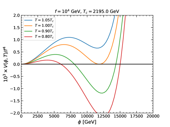
Figure 1: Evolution of the effective potential with temperature, taking $f=10^{4}$ GeV, $\kappa_{m}=0.15$, $\kappa_{l}=0.10$, and $\varepsilon=0.51$.

The phase transition would be first-order if there exists a sufficiently high and wide potential barrier separating the two degenerate vacua of the thermal effective potential at the critical temperature. As shown in section 3.2, adding a dimension-6 operator could make the self-coupling $\lambda$ negative. The tree-level barrier could then arise if the parameter $m^{2}$ is negative (or $d^{2}V(0,T)/d\phi^{2}>0$) at the same time. The gear fields can make contributions to the barrier of the effective potential at loop level. This is given by the third term on the right hand side of the improved high temperature expansion (3.24). In Fig. 1, we show the evolution of the potential with temperature, using the parameters $f=10^{4}$ GeV, $\kappa_{m}=0.15$, $\kappa_{l}=0.10$, and $\varepsilon=0.51$. As shown in the figure, the two vacua become degenerate at the critical temperature $T_{c}=2.195$ TeV and there is a potential barrier between the two vacua.

In search of parameter space that permits a first-order phase transition, we take $f=10^{4}$ GeV and make a random scan of the parameters in the following ranges:

$$10^{-3}\leq\kappa_{m}\leq 1~{},~{}~{}10^{-3}\leq\kappa_{l}\leq 1~{},~{}{\rm and}~{}~{}10^{-3}\leq\varepsilon\leq 1~{}.$$ (3.25)

The upper value of $\kappa_{l}$ is required by $f\leq\Lambda$ and the upper limit on $\varepsilon$ is to ensure the perturbativity of theory. Given a set of parameters, we first check various constraints discussed above. We start from an initial temperature given by eq. (3.19) and find the local VEV minimum around the value given by eq. (3.20). If the local minimum at the symmetric phase $\phi(T)=0$ is found to be larger (smaller) than the one at the broken phase $\phi(T)\neq 0$, the temperature is increased (decreased) in the next trial. The critical temperature is then determined by the degenerate condition i.e., $V(0,T_{c})=V(\phi_{c},T_{c})$. We find that for most of the sample points, the VEV at critical temperature is larger than that given by eq. (3.20). We generate one million random floats uniformly for each of the input parameters, among which about 4.8% are found to be able to trigger afirst-order phase transition.

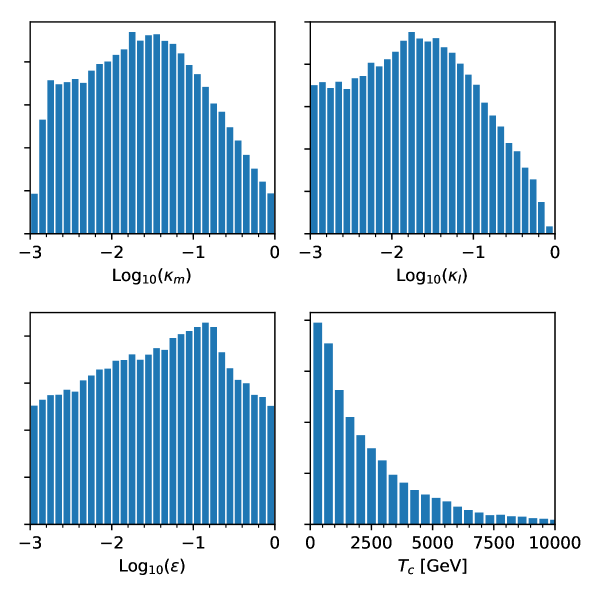
Figure 2: Distributions of the parameters that can trigger a first-order phase transition and the critical temperature distribution. The symmetry breaking scale is fixed at $f=10^{4}$ GeV.

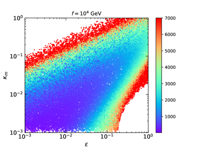
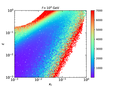
Figure 3: Scatter plots of parameter distributions in the $\varepsilon-\kappa_{m}$ and $\kappa_{l}-\varepsilon$ planes. The color represents the critical temperature in units of GeV.

Fig. 2 shows the distributions of the parameters and the critical temperature. We have fixed the parameter $f=10^{4}$ GeV. For other choices of $f$, the distributions are found to be nearly the same. We observe that the distribution profile of $\kappa_{m}$ is similar to that of $\kappa_{l}$. This is because of the requirement $\kappa_{l}\lesssim\kappa_{m}$ from the above discussions. The parameter $\varepsilon$ mainly peaks around 0.1. The distribution of the critical temperature concentrates in $\lesssim 2.5$ TeV and decreases quickly with the temperature. Finally, we plot the scatter distributions on the $\varepsilon-\kappa_{m}$ and $\kappa_{l}-\varepsilon$ plane in Fig. 3, from which we can directly observe the variation of the critical temperature with respect to the parameters.

We note that the existence of two degenerate vacua at the critical temperature does not guarantee that a first-order phase transition could successfully happen. To achieve a successful first-order phase transition, the bubble nucleation of the true vacuum should be triggered successfully as the temperature of the Universe drops from $T_{c}$ to a certain value. This will further constrain the parameter space for the phase transition, as will be discussed in the next section.

4 Bubble nucleation

At high temperatures the Universe is in the symmetric phase, where the vacuum is located at the origin of the scalar field. As the temperature decreases with the expansion of the Universe, the other minimum of the effective potential appears and becomes the global minimum when the temperature goes lower than critical temperature. For a first-order phase transition, the symmetric and broken vacua are separated by a potential barrier. The tunneling from the metastable minimum to the stable one can proceed through the help of thermal fluctuations. The tunneling process leads to the decay of the false vacuum and the nucleation of the true vacuum. The tunneling rate per unit volume and time element is approximately given by [84, 4]

$$\Gamma(T)=A(T)e^{-S_{3}/T}~{},$$ (4.1)

where $A(T)\simeq[S_{3}/(2\pi T)]^{3/2}T^{4}$ and $S_{3}$ denotes the three-dimensional on-shell Euclidean action of instanton. The probability of bubble nucleations per Hubble volume is defined as

$$p(T)=\int_{T}^{T_{\rm c}}\frac{\Gamma(x)}{H^{4}(x)}\frac{dx}{x}\approx\left(\frac{T}{H}\right)^{4}e^{-S_{3}/T}~{}.$$ (4.2)

In a radiation dominated Universe, the Hubble parameter is given by

$$H=1.66g_{*}^{1/2}T^{2}/M_{\mathrm{pl}}~{},$$ (4.3)

where $g_{\ast}\simeq 110$ and $M_{\rm pl}=1.22\times 10^{19}$ GeV is the Planck mass. The potential barrier decreases with the decrease of the temperature, which improves the probability of the vacuum tunneling. The nucleation temperature $T_{\rm n}$ is defined to be one at which the probability of nucleating one bubble per horizon volume is of order one, i.e., $p(T)\sim 1$, which can be translated into the following criterion for determining the nucleation temperature [4]

$$\frac{S_{3}(T_{\rm n})}{T_{\rm n}}\simeq 4\ln\left(\frac{T_{\rm n}}{H}\right)~{}.$$ (4.4)

For a successful bubble nucleation, the tunneling rate from the flase vacuum to the true vacuum should be large enough to overcome the expansion rate of the Universe. It is this criterion that determines whether the first-order cosmological phase transition has successfully proceeded or not. We see that, for one thing, a first-order phase transition needs a barrier to separate the two vacua. This has been fully explored in section 3. For another thing, the proceeding of the bubble nucleation may be hindered if the barrier is too high or the decrease of the barrier with temperature is too slow. In the following, we will determine the parameter space that satisfies the bubble nucleation criterion.

To determine the bubble nucleation, we have to first obtain the Euclidean action of the $O(3)$ symmetric field configuration $S_{3}(T)$, which can be written as

$$S_{3}(T)=4\pi\int dr~{}r^{2}\left[\frac{1}{2}\left(\frac{d\phi}{dr}\right)^{2}+V_{\rm eff}(\phi,T)\right]~{}.$$ (4.5)

By extremizing the Euclidean action, we obtain the following differential equation

$$\frac{d^{2}\phi}{dr^{2}}+\frac{2}{r}\frac{d\phi}{dr}-\frac{dV}{d\phi}=0~{},$$ (4.6)

with the boundary conditions

$$\left.\frac{d\phi}{dr}\right|_{r=0}=0,\quad\lim_{r\rightarrow\infty}\phi(r)=\phi_{\mathrm{false}}\equiv 0~{}.$$ (4.7)

The equation of motion, eq. (4.6), can be solved by the traditional overshooting/undershooting method [84]. In this work, we employ the CosmoTransitions 2.0.2 package [85] to perform the numerical calculations of the bubble profile and Euclidean action. Afterwards, we use eq. (4.4) to determine the nucleation temperature $T_{n}$. The first-order phase transition is usually completed after percolation of the true vacuum bubbles. The production of GWs is significant at the percolation time (temperature), at which 34% of the false vacuum has been converted to the true vacuum [35, 65, 86]. In this work, we assume that the percolation takes place soon after the nucleation of the true vacua, which leads to the commonly used condition $T_{*}\simeq T_{n}$, where $T_{*}$ is the GW generation temperature [4, 87].

The stochastic GWs generated by the first-order phase transition can be fully characterized by the knowledge of two primary parameters [88]. One of them is the latent heat normalized by the radiation energy density in the plasma

$$\alpha=\frac{\epsilon(T_{n})}{\rho_{\rm rad}(T_{n})}~{},$$ (4.8)

where $\rho_{\rm rad}=\pi^{2}g_{\ast}T^{4}/30$ is the radiation energy density in the plasma, and the latent heat associated with the phase transition is given by

$$\epsilon(T)=T\frac{\partial\Delta V_{bs}(T)}{\partial T}-\Delta V_{bs}(T)~{},$$ (4.9)

where $\Delta V_{bs}(T)\equiv V_{\rm eff}(f(T),T)-V_{\rm eff}(0,T)$ is the potential difference between the broken phase and the symmetric phase at temperature $T$. The parameter $\alpha$ is related to the maximum available energy budget for gravitational wave emissions. The other parameter relevant to the GW production is defined as

$$\frac{\beta}{H_{n}}=\left.T_{n}\frac{d}{dT}\left(\frac{S_{3}(T)}{T}\right)\right|_{T=T_{n}}~{}.$$ (4.10)

The parameter $\beta$ represents the rate of time variation of the nucleation rate, whose inverse gives the duration of the bubble nucleation. Consequently, $\beta/H_{n}$ defines the characteristic frequency of the GW spectrum produced from the phase transition.

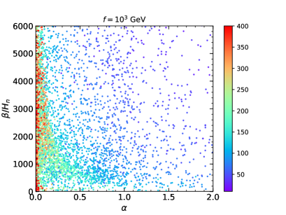
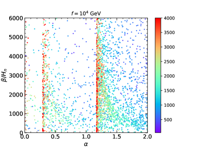
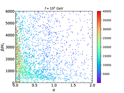
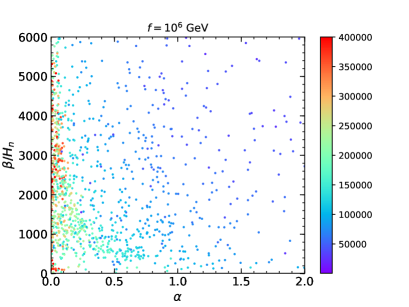
Figure 4: Distributions of the GW parameters $\alpha$ and $\beta/H_{n}$. The color bars indicate the nucleation temperature. For the upper left, upper right, lower left and lower right plots, the symmetry breaking scales are taken as $f=10^{3}$ GeV, $10^{4}$ GeV, $10^{5}$ GeV, and $10^{6}$ GeV, respectively.

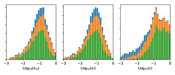
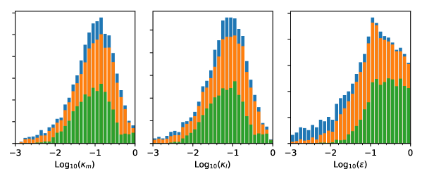
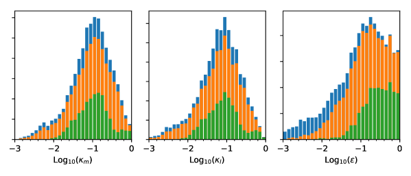
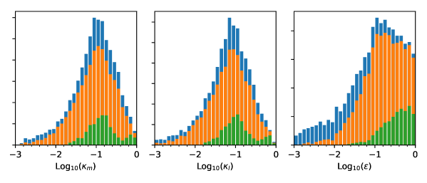
Figure 5: Histograms of the parameters that satisfy the nucleation condition. The blue histograms represent the total samples, and the orange and green histograms denote those samples that are detectable by the BBO and LISA interferometers, respectively. From top to bottom, the symmetry breaking scales are fixed at $f=10^{3}$ GeV, $10^{4}$ GeV, $10^{5}$ GeV, and $10^{6}$ GeV.

In the scatter plots of Fig. 4, we show the calculated results of $\alpha$ and $\beta/H_{n}$, with the the corresponding nucleation temperature $T_{n}$ indicated by the colored dots. We find about 15% of the sample points that trigger a first-order phase transition (see Fig. 2) can also satisfy the bubble nucleation condition. The plot shows that the nucleation temperature tends to be lower for larger $\alpha$, in agreement with the observation that the GWs can be stronger when they are produced at a lower nucleation temperature [65, 87, 89]. The distributions of parameters $\kappa_{m}$, $\kappa_{l}$, and $\varepsilon$ are shown by the blue histograms in Fig. 5. From the upper plots to the lower plots, the $U(1)$ symmetry breaking scale $f$ is taken as $10^{3}$ GeV, $10^{4}$ GeV, $10^{5}$ GeV, and $10^{6}$ GeV, respectively. Compared with the parameter distributions for generating a first-order phase transition, as shown in Fig. 2, $\kappa_{m}$, $\kappa_{l}$, and $\varepsilon$ have been restricted to be $\gtrsim 10^{-2}$ by the criterion of the successful bubble nucleation.

5 Gravitational waves from phase transition

5.1 Gravitational wave sources

We first briefly review the numerical simulation results of the GW spectra produced from a first-order phase transition. During the percolation of the bubbles, there exist three processes that can produce the GWs [90, 91, 92]:

• Bubble Collisions. GWs produced from this process depends only on the dynamics of the scalar field. The GW spectrum from the collisions of bubble walls estimated by the numerical simulations [93] is given by

  $$h^{2}\Omega_{\mathrm{\rm col}}(f)=1.67\times 10^{-5}\left(\frac{H_{n}}{\beta}\right)^{2}\left(\frac{\kappa_{\rm col}\alpha}{1+\alpha}\right)^{2}\left(\frac{100}{g_{*}}\right)^{\frac{1}{3}}\left(\frac{0.11v_{w}^{3}}{0.42+v_{w}^{2}}\right)\frac{3.8\left(f/f_{\mathrm{col}}\right)^{2.8}}{1+2.8\left(f/f_{\mathrm{col}}\right)^{3.8}}~{},$$ (5.1)

  where the red-shifted peak frequency of the GW spectrum from bubble collision is

  $$f_{\mathrm{col}}=16.5\times 10^{-3}\mathrm{mHz}\left(\frac{0.62}{1.8-0.1v_{w}+v_{w}^{2}}\right)\left(\frac{\beta}{H_{n}}\right)\left(\frac{T_{n}}{100\mathrm{GeV}}\right)\left(\frac{g_{*}}{100}\right)^{\frac{1}{6}}~{}.$$ (5.2)

  The efficiency factors $\kappa_{\rm col}$ indicates the fraction of latent heat that is transformed into the kinetic energy of bubbles. In the case of non-runaway bubbles, the bubble walls will reach a terminal velocity and the latent energy transferred into the scalar field is negligible. For the runaway bubbles, however, most of the bubble energy is dissipated into the surrounding plasma and very little energy is deposited in the bubble walls [94]. Both cases lead to a negligible GW spectrum from the bubble collisions, and thus, in this work we do not take into account the bubble collision’s contributions. In the following, we will restrict ourselfs to the case of non-runaway bubbles, in which the GWs can be effectively produced by the sound waves and turbulence.

• Sound waves. They are generated subsequently after the bubble collisions. Numerical simulations indicate that the durations of sound waves and turbulence as active sources of GWs are typically much longer than the collisions of the bubble walls. The GW spectrum generated by sound waves propagating in the plasma is approximated by [95]

  $$h^{2}\Omega_{\mathrm{sw}}(f)=2.65\times 10^{-6}\left(\frac{H_{*}}{\beta}\right)\left(\frac{\kappa_{\rm sw}\alpha}{1+\alpha}\right)^{2}\left(\frac{100}{g_{*}}\right)^{\frac{1}{3}}v_{w}\left(\frac{f}{f_{\rm{sw}}}\right)^{3}\left(\frac{7}{4+3\left(f/f_{\mathrm{sw}}\right)^{2}}\right)^{7/2},$$ (5.3)

  where the red-shifted peak frequency of the GW spectrum from sound waves is

  $$f_{\mathrm{sw}}=1.9\times 10^{-2}\mathrm{mHz}\frac{1}{v_{w}}\left(\frac{\beta}{H_{n}}\right)\left(\frac{T_{n}}{100\mathrm{GeV}}\right)\left(\frac{g_{*}}{100}\right)^{\frac{1}{6}}.$$ (5.4)

  The efficiency factors $\kappa_{\rm sw}$ indicates the fraction of latent heat that is transformed into the bulk motion of the plasma. For the non-runaway bubbles, the efficiency factor for the sound wave contribution is then given by

  $$\kappa_{\mathrm{sw}}\simeq\frac{\alpha}{0.73+0.083\sqrt{\alpha}+\alpha}~{},~{}~{}{\rm for}~{}~{}v_{w}\sim 1.0~{}.$$ (5.5)

• Turbulence. As the sound waves, turbulence in the plasma forms after the bubble collisions. Simulations show that only a small fraction $\delta\sim 5-10\%$ of the bulk motion from the bubble walls is converted into turbulence. Since the GWs from sound waves decay much faster, the GWs from turbulence could play a dominant role at high frequencies. The modeling of turbulence is far from settled. In this work, we adopt GW spectrum from turbulence as follows [96]

  $$h^{2}\Omega_{\mathrm{turb}}(f)=3.35\times 10^{-4}\left(\frac{H_{*}}{\beta}\right)\left(\frac{\kappa_{\mathrm{turb}}\alpha}{1+\alpha}\right)^{\frac{3}{2}}\left(\frac{100}{g_{*}}\right)^{1/3}v_{w}\frac{\left(\frac{f}{f_{\mathrm{turb}}}\right)^{3}}{\left[1+\frac{f}{f_{\mathrm{turb}}}\right]^{\frac{11}{3}}\left(1+\frac{8\pi f}{H_{0}}\right)}~{},$$ (5.6)

  where the red-shifted Hubble constant observed today is given by

  $$H_{0}=16.5\times 10^{-3}\mathrm{mHz}\left(\frac{T_{n}}{100\mathrm{GeV}}\right)\left(\frac{g_{*}}{100}\right)^{\frac{1}{6}}.$$ (5.7)

  The red-shifted peak frequency of the GW spectrum from turbulence is

  $$f_{\text{turb }}=2.7\times 10^{-2}\mathrm{mHz}\frac{1}{v_{w}}\left(\frac{\beta}{H_{n}}\right)\left(\frac{T_{n}}{100\mathrm{GeV}}\right)\left(\frac{g_{*}}{100}\right)^{\frac{1}{6}}.$$ (5.8)

  The efficiency factor for turbulence $\kappa_{\rm turb}$ is related to $\kappa_{\rm sw}$ by $\kappa_{\rm turb}=\delta\kappa_{\rm sw}$, where we take $\delta=0.1$ in this work.

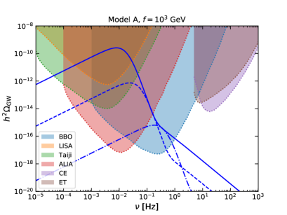
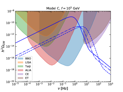
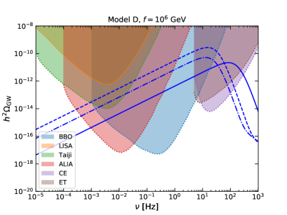
Figure 6: GW spectra from phase transition (curves) and various experimental sensitivities (colored patches) as a function of frequency. The solid, dashed, and dash-dotted curves represent the results in model $\rm M_{1}$, $\rm M_{2}$, and $\rm M_{3}$ (where M=A, B, C, and D). For the upper left, upper right, lower left and lower right plots, the symmetry breaking scales are taken as $f=10^{3}$ GeV, $10^{4}$ GeV, $10^{5}$ GeV, and $10^{6}$ GeV, respectively. The parameters used in this plots are summarized in Table. 1.

The amplitude and peak frequency of the GW spectrum also depend on the bubble wall velocity $v_{w}$, which is the expanding speed of the true vacuum. In this work, we take $v_{w}\simeq 1.0$ for the calculations of GW spectra. The total stochastic GW spectrum is approximately given by adding up these three contributions:

$$h^{2}\Omega_{\mathrm{GW}}\simeq h^{2}\Omega_{\rm col}+h^{2}\Omega_{\mathrm{sw}}+h^{2}\Omega_{\mathrm{turb}}.$$ (5.9)

Note that as explained above, the bubble collision’s contribution has been neglected in our calculation.

5.2 Gravitational wave detections

For the experimental investigation of the stochastic GW signals, one often adopts the frequentist approach where the detectability of the signals is measured by the corresponding signal-to-noise ratio (SNR) [92]

$$\rho=\sqrt{\mathcal{N}\mathcal{T}_{\rm obs}\int_{f_{\mathrm{min}}}^{f_{\mathrm{max}}}df\left[\frac{h^{2}\Omega_{\mathrm{GW}}(f)}{h^{2}\Omega_{\mathrm{exp}}(f)}\right]^{2}}~{},$$ (5.10)

where $\mathcal{N}$ is the number of independent observatories of the experiment, $\mathcal{T}_{\rm obs}$ is the duration of the mission, and $h^{2}\Omega_{\mathrm{exp}}$ denotes the sensitivity of a GW experiment. Following ref. [92], we take the SNR threshold value $\rho_{\rm thr}=10$, above which the GW signal is detectable for the experiment.

The future space-based GW interferometers, including LISA [66, 67], Taiji [68, 69], ALIA [70], DECIGO [71], and BBO [72] are able to explore the GW signals with the frequencies in the range of $\sim 10^{-5}-10^{2}$ Hz. Higher frequencies ($\sim 10-10^{3}$ Hz) GW signals are expected to be probed by the ground-based GW observatories such as aLIGO [75], ET [73], and CE [74].

We show the distributions of parameters with detectibility for BBO and LISA interferometers in Fig. 5. We use $\mathcal{N}=1$ for the auto-correlated experiment, LISA, while for the cross-correlated experiments, BBO, we take $\mathcal{N}=2$. Following ref. [32], we assume a mission duration of $\mathcal{T}_{\rm obs}=4$ years for both interferometers. The observation frequency ranges are set in the range of $10^{-3}-10^{2}$ and $10^{-5}-1$ Hz for BBO and LISA, respectively. The experimental sensitivities of BBO and LISA are summarized in appendix E of ref. [32]. The orange and green histograms represent the detectable regions for BBO and LISA, respectively. As indicated in the figure, the BBO experiment can probe almost all of the parameter space that can successfully generate a first-order phase transition. The GW signals produced at the scale $f=10^{3}$ GeV in the clockwork model can be effectively detected by the LISA experiment. The nucleation temperature increases with $f$, leading to higher peak frequencies of the GW signals. As a result, it is difficult to probe the GW signals induced by the $U(1)$ symmetry breaking at a scale of $f=10^{6}$ GeV at the LISA interferometer. We will show in section 6 that the domain walls produced after the phase transition at the symmetry breaking scale $f\gtrsim 10^{6}$ GeV could dominate the energy density of the Universe, which is not compatible with cosmological observations. Thus, here we do not further consider those GW signals produced from the phase transition above the scale of $f=10^{6}$ GeV.

Table 1: A summary of models and parameters

	Models	$\kappa_{m}$	$\kappa_{l}$	$\varepsilon$	$T_{c}$ [GeV]	$T_{n}$ [GeV]	$\alpha$	$\beta/H_{n}$
Model A $f=10^{3}$ GeV	$\rm A_{1}$	0.176	0.128	0.548	231.4	115.4	0.715	751.4
	$\rm A_{2}$	0.120	0.092	0.094	207.1	126.6	0.133	2046.6
	$\rm A_{3}$	0.449	0.332	0.309	417.9	383.3	0.025	5188.6
Model B $f=10^{4}$ GeV	$\rm B_{1}$	0.228	0.181	0.440	2287.3	969.2	1.220	348.2
	$\rm B_{2}$	0.080	0.053	0.511	2524.1	645.5	0.261	1163.0
	$\rm B_{3}$	0.101	0.071	0.086	1979.4	1597.2	0.054	4877.7
Model C $f=10^{5}$ GeV	$\rm C_{1}$	0.151	0.115	0.538	21686.2	8087.8	1.472	660.1
	$\rm C_{2}$	0.029	0.019	0.092	9494.1	4607.1	0.763	9355.4
	$\rm C_{3}$	0.317	0.227	0.807	29054.8	20595.1	0.307	907.8
Model D $f=10^{6}$ GeV	$\rm D_{1}$	0.018	0.015	0.018	70698.9	23487.0	1.658	39613.7
	$\rm D_{2}$	0.071	0.055	0.173	136258.8	50724.8	1.698	3261.5
	$\rm D_{3}$	0.262	0.187	0.714	270259.0	176070.9	0.380	791.0

In Fig. 6 we plot the GW spectrum as a function of frequency, with various choices of parameters shown in Table 1. The solid, dashed, and dash-dotted curves depict the spectra expected for model $\rm M_{1}$, $\rm M_{2}$, and $\rm M_{3}$, where M=A, B, C, and D. The upper left, upper right, lower left and lower right plots assume the symmetry breaking scales of $f=10^{3}$ GeV, $10^{4}$ GeV, $10^{5}$ GeV, and $10^{6}$ GeV, respectively. As shown in the plots, the peak frequency increases with the symmetry breaking scale. We observe that the $U(1)$ symmetry breaking scales in the range of $10^{3}-10^{6}$ GeV are all within the probe of the BBO and ALIA interferometers. The LISA and Taiji interferometers can probe lower frequencies of GW signals, corresponding to the symmetry breaking scale $f\lesssim 10^{4}$ GeV. On the other hand, the GW signals from scale of $f=10^{6}$ GeV could be detected by the ground-based GW observatories ET and CE.

5.3 LIGO searches on stochastic gravitational waves

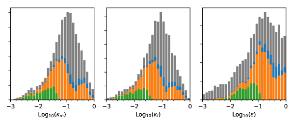
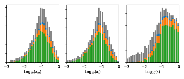
Figure 7: Histograms of the parameters that satisfy the nucleation condition. The grey histograms represent the total samples, and the blue, orange, and green histograms denote those samples that can be probed for LIGO design, O3, and O2 run, respectively. The top (bottom) row assumes the symmetry breaking scale to be $10^{5}$ GeV (and $10^{6}$ GeV).

We have shown that for the symmetry breaking scale at $f\sim 10^{6}$ GeV, the peak frequencies of the GW signals are right in the range that is covered by the ground-based GW observatories. Searches for the isotropic stochastic GWs background have been undertaken by the LIGO and Virgo Collaborations. The results from a cross-correlation analysis of data from the two observing run phases (O1 and O2) of Advanced LIGO are shown in refs. [76, 77]. The upper limits on the normalized energy density in GWs at the 95% confidence level of $\Omega_{\rm GW}<6.0\times 10^{-8}$ at 25 Hz for a flat background have been obtained due to no evidence for the existence of a stochastic background.

Here we take advantage of the results from the Advanced LIGO O2 running to put constraints on the clockwork axion model. We will also estimate the detection prospects for the on-going Advanced LIGO observing run, including the third phase (O3) and design phase. The second observing run, O2, has ben completed in 2017 and ran for approximately 9 months. Following ref. [76], we use a duration of 12 months for O3 run and assume 24 months for the design phase (2022+). The GW background may be detectable with a $\rm SNR=3$ [76].

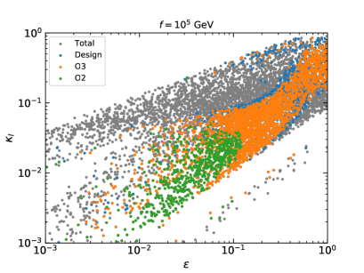
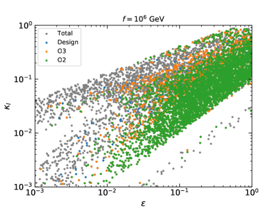
Figure 8: Scatter plots of the parameter distributions on the $\varepsilon-\kappa_{l}$ plane. The grey scatter dots represent the total samples that satisfy the nucleation condition, while the blue, orange, and green scatter dots denote those samples that can be probed by the LIGO design, O3, and O2 run, respectively. We fix $f=10^{5}$ GeV and $10^{6}$ GeV in the left and right plots, respectively.

We calculate the GW signals from the vacuum phase transitions at all sites, assuming $N=10$, and compare them with the LIGO sensitivities. The main results are shown in Fig. 7 and Fig. 8. The green, orange and blue histograms in Fig. 7 represent detection ranges in the O2, O3 and design phases, respectively. The grey histograms are the total samples that can generate a successful phase transition. We fix the symmetry breaking scale to $f=10^{5}$ GeV and $10^{6}$ GeV in the upper and lower plots of Fig. 7, respectively. We further show the detectable regions for the LIGO run phases on the $\varepsilon-\kappa_{l}$ plane in Fig. 8. Since no evidence for a stochastic GW background is found in the O2 run of LIGO, we interpret the green histograms in Fig. 7 (and scatter points in Fig. 8) as those parameter regions that have been constrained by the LIGO O2 observations. Combine with Fig. 7 and Fig. 8, we observe that for the symmetry breaking scale of $f=10^{5}$ GeV, the parameter space with $\kappa_{m}\sim 0.06-0.001$, $\kappa_{l}\sim 0.04-0.001$, and $\varepsilon\sim 0.1-0.01$ has been excluded by LIGO O2 run. Nearly half of the parameter space for $f=10^{5}$ GeV can be further tested by LIGO O3 and design phases.

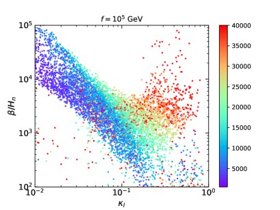
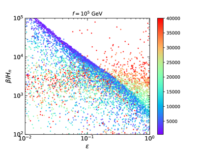
Figure 9: The distribution of $\beta/H_{n}$ as a function of $\kappa_{l}$ (left) and $\varepsilon$ (right). The colored bars represent the nucleation temperature. We fix $f=10^{5}$ GeV, and $10^{6}$ GeV in the left and right plot, respectively.

To see why lower values of $\kappa_{m}$, $\kappa_{l}$, and $\varepsilon$ for $f=10^{5}$ GeV can be effectively probed by the LIGO O2 run, we plot in Fig. 9 the parameter $\beta/H_{n}$ as a function of the parameters $\kappa_{l}$ (left) and $\varepsilon$ (right), with the color indicating the nucleation temperature. We observe that $T_{n}$ tends to increase with both $\kappa_{l}$ and $\varepsilon$, while $\beta/H_{n}$ tends to decrease as $\kappa_{l}$ and $\varepsilon$ increase. For the parameters in the available range of O2 run, we find $T_{n}\lesssim 10^{4}$ GeV and $\beta/H_{n}\gtrsim 5\times 10^{3}$. With eq. (5.8), the peak frequencies for these parameters fall in the range of $10-100$ Hz, which are the most sensitive frequency band for LIGO. However the amplitude of GW signal is suppressed by a large value of $\beta/H_{n}$ since $h^{2}\Omega_{\rm GW}$ is inversely proportional to $\beta/H_{n}$ (with bubble collisions being neglected). For the case of $f=10^{6}$ GeV, we can achieve the LIGO sensitive frequency band with a higher nucleation temperature $T_{n}\gtrsim 10^{5}$ GeV and a lower $\beta/H_{n}\lesssim 5\times 10^{2}$. Thus, the GW signals from symmetry breaking at the scale $f=10^{6}$ GeV can be sufficiently loud for LIGO O2 run, as indicated the Fig. 7 and Fig. 8. We observe that for $f=10^{6}$ GeV, most of the parameter space has been excluded by while the LIGO O2 run, the remaining regions can be further tested by LIGO O3 and design phases.

6 Gravitational waves from domain wall annihilation

6.1 Gravitational wave spectrum

The network of cosmic strings and domain walls form after the phase transition of the clockwork axion model. Numerical simulations [55] show that for large number of $N$ ($\gtrsim 3$), this string-wall network can survive until the QCD phase transition. The QCD instanton effects at $T\lesssim 1$ GeV give rise to the QCD axion potential, $V_{\rm bias}\sim\Lambda_{\rm QCD}^{4}$ (where $\Lambda_{\rm QCD}=(332\pm 17)$ MeV [97] is the the QCD confinement scale), which serves as an energy bias to break the degeneracy of discrete vacua, and thus, leads to the annihilation of the domian walls.

In the scaling regime for long-lived domain walls, the evolution of the energy density of domain walls can be parameterized as

$$\rho_{\rm wall}(t)=\mathcal{A}\frac{\sigma}{t}~{},$$ (6.1)

where $\sigma\simeq 8m_{A}^{2}f^{2}$ is the tension of the domain wall [55, 58], $t=1/(2H)$, and $\mathcal{A}\sim 1.0$ from the analysis of numerical simulations [98]. The annihilation of domain walls becomes significant when the tension of domain walls is comparable with the volume pressure $p_{\rm V}\sim V_{\rm bias}$, and the annihilation temperature of domain walls is given by [99]

$$T_{\rm ann}\simeq 7.15\times 10^{-2}~{}{\rm GeV}~{}\varepsilon^{-1/4}\left(\frac{g_{*}\left(T_{\mathrm{ann}}\right)}{10}\right)^{-1/4}\left(\frac{f}{100~{}\rm{TeV}}\right)^{-3/2}\left(\frac{\Lambda_{\rm QCD}}{100~{}\rm{MeV}}\right)^{2}.$$ (6.2)

Eq. (6.1) shows that the energy density of domain walls in the scaling regime decreases as $\propto t^{-1}$. This decay rate is slower than those of dusts $\propto t^{-3/2}$ and radiation $\propto t^{-2}$. From the condition $\rho_{c}=\rho_{\rm wall}$, where $\rho_{c}$ is the critical density of the Universe, the energy density of the Universe would eventually be dominated by the domain walls at the temperature

$$T_{\rm dom}=5.44\times 10^{-2}~{}{\rm GeV}~{}\varepsilon^{1/4}\left(\frac{g_{*}\left(T_{\mathrm{ann}}\right)}{10}\right)^{-1/4}\left(\frac{f}{100~{}\rm{TeV}}\right)^{3/2}.$$ (6.3)

Requiring the domain walls annihilate before they dominate the Universe, i.e., $T_{\rm ann}\gtrsim T_{\rm dom}$, we have

$$f\lesssim 100~{}{\rm TeV}~{}\varepsilon^{-1/6}\left(\frac{\Lambda_{\rm QCD}}{100~{}\rm{MeV}}\right)^{2/3}.$$ (6.4)

We thus find an upper bound on the symmetry breaking scale, $f\lesssim 400$ TeV.

The production of GWs from the annihilation of domain walls has been studied in the literature. The peak amplitude of the GW spectrum is produced at the annihilation time of domain walls,

$$\Omega_{\mathrm{GW}}\left(\nu_{\mathrm{peak}}\left(t_{\mathrm{ann}}\right)\right)\simeq\frac{8\pi\tilde{\epsilon}_{\mathrm{gw}}G^{2}A^{2}\sigma^{2}}{3H_{\mathrm{ann}}^{2}}~{},$$ (6.5)

where the efficiency of the gravitational wave emission $\tilde{\epsilon}_{\rm{gw}}\simeq 0.7\pm 0.4$ [100] and $A\simeq N$ from the numerical simulations [55]. With the expansion of the Universe, the amplitude is diluted as $\propto R(t)^{-4}$, where $R(t)$ is the scale of the Universe. The peak amplitude of the GW spectrum today is given by

$$h^{2}\Omega_{\rm{GW}}^{\rm peak}\left(t_{0}\right)=6.45\times 10^{-6}\varepsilon\left(\frac{\tilde{\epsilon}_{\rm{gw}}}{0.7}\right)\left(\frac{A}{10}\right)^{2}\left(\frac{g_{*s}\left(T_{\rm{ann}}\right)}{10}\right)^{-4/3}\left(\frac{f}{100~{}\rm{TeV}}\right)^{6}\left(\frac{T_{\rm{ann}}}{0.1~{}\rm{GeV}}\right)^{-4},$$ (6.6)

with the red-shifted peak frequency from $\nu_{\rm{peak}}\left(t_{\rm{ann}}\right)\simeq H_{\rm{ann}}$ given by

$$\nu_{\rm peak}(t_{0})\simeq 1.1\times 10^{-8}\mathrm{~{}Hz}\left(\frac{g_{*}\left(T_{\mathrm{ann}}\right)}{10}\right)^{1/2}\left(\frac{g_{*s}\left(T_{\mathrm{ann}}\right)}{10}\right)^{-1/3}\left(\frac{T_{\mathrm{ann}}}{0.1~{}\rm{GeV}}\right).$$ (6.7)

The analysis of numerical simulations in ref. [100] shows that the frequency dependence of the GW spectrum can be approximately parameterized as

$$h^{2}\Omega_{\rm GW}=\begin{cases}\displaystyle h^{2}\Omega_{\rm GW}^{\rm peak}\left(\nu\over\nu_{\rm peak}\right)^{3}~{}{\rm for~{}\nu<\nu_{\rm peak}}\\ \displaystyle h^{2}\Omega_{\rm GW}^{\rm peak}\left(\nu_{\rm peak}\over\nu\right)~{}~{}{\rm for~{}\nu>\nu_{\rm peak}}.\end{cases}$$ (6.8)

6.2 NANOGrav pulsar timing observations

The byproducts of the clockwork axion phase transition, the domain walls, dominantly annihilate at a temperature around $T_{\rm ann}\sim 0.1-1$ GeV, right after the QCD confinement. From eq. (6.7), we see that the peak frequency of GWs from domain wall annihilation is around $\sim 10^{-8}$ Hz, falling in the frequency band probed by pulsar timing observations. The searches for nHz isotropic stochastic GW background via the observation of pulsars are performing by, for example, the European Pulsar Timing Array (EPTA) [101] and the NANOGrav [102], over a long time span. The constraints from the observations of 18 years by EPTA and over 11 years by NANOGrav have restricted the GW background amplitude in the frequency band of $2-10$ nHz to be $h^{2}\Omega_{\rm GW}\lesssim 5\times 10^{-9}$ and $10^{-9}$, respectively. These results constrain the symmetry breaking scale to be $f\lesssim 300$ TeV, slightly tighter than the constraints from requiring domain walls to annihilate before they dominate the energy density of the Universe.

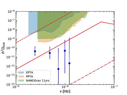
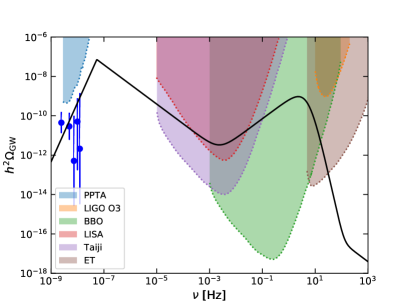
Figure 10: The GW spectra and various experimental sensitivities as a function of frequency. In both plots, the blue data points represent the analysis of NANOGrav 12.5-year data, the parameter is fixed at $\kappa_{m}=0.030$, $\kappa_{l}=0.024$, and $\varepsilon=0.1$, respectively. In the left plot, the red dashed, solid, and dashed-dot lines represent the GW spectrum from domain wall annihilation with a symmetry breaking scale $f=300$ TeV, $f=200$ TeV, and $f=100$ TeV, respectively. The black line in the right plot shows the total GW signal from domain wall annihilation and first-order phase transition.

The NANOGrav Collaboration has recently released their analysis on the 12.5-year data [78] and one signal of a stochastic spectrum was found within the frequency band $\sim 1-10$ nHz. Various possible sources of the signal have been proposed, including cosmic strings [103, 104, 105, 106], first-order cosmological phase transitions [107, 108, 109, 110, 111, 112], coherent oscillation of axionic fields [113, 114], and primordial black holes [115, 115, 117]. As indicated by eq. (6.7), the nHz stochastic GWs can naturally be produced by the annihilation of domain walls in the clockwork axion model [55]. In the left plot of Fig. 10, we show the GW relic energy density from the domain wall annihilation, taking $\varepsilon=0.1$. The red dashed, solid, and dash-dotted lines represent the results with a symmetry breaking scale of $f=300$ TeV, $f=200$ TeV, and $f=100$ TeV, respectively. We find that GWs from the model with a scale $f=200$ TeV can explain the NANOGrav 12.5-year data in blue points. In addition to the nHz GW signals, the first-order phase transition of the clockwork work axion model at the scale of $f=200$ TeV can also produce a GW signal peaked around $\sim 10$ Hz. We show the result in this scenario with the black line in the right plot of Fig. 10. As we have shown in the previous section, most of the parameter space for the first-order phase transition at the scale $f=10^{3}$ TeV has been excluded by the LIGO O2 run. The O3 and the design phases of LIGO could probe half of the parameter space of the phase transition at the scale around $10^{2}$ TeV. We thus expected another signal in the LIGO O3 run if the NANOGrav 12.5-year data are indeed induced by the annihilation of domain walls from the phase transition of the clockwork work axion at the scale of $f=200$ TeV.

7 Conclusions

We have shown in this work the opportunity to explore the clockwork axion with the information from gravitational wave (GW) detection. It is well known that GWs can be produced from violent first-order cosmological phase transitions. However, in the conventional QCD axion models the PQ phase transition is second-order. We show that the PQ phase transition can be first-order when the dimension-6 operator is included in the scalar potential. Based on a comprehensive scan in the parameter space, we find that the parameters $\kappa_{m}$, $\kappa_{l}$, and $\varepsilon$ have been restricted within the range of $10^{-2}-1.0$ in order to trigger a first-order phase transition while having successful nucleation of the true vacuum bubble. We show that the GWs from the PQ phase transition at scales in the range of $10^{3}-10^{6}$ GeV can be probed by the BBO and ALIA interferometers. The LISA and Taiji interferometers could probe GW signals of lower frequencies, corresponding to the symmetry breaking scale of $f\lesssim 10^{4}$ GeV. On the other hand, the GW signals from the scale $f\gtrsim 10^{5}$ GeV could be detected by the ground-based GW observatories ET and CE. In fact, we find that for the symmetry breaking scale of $f=10^{5}$ GeV, the parameter space of $\kappa_{m}\sim 0.06-0.001$, $\kappa_{l}\sim 0.04-0.001$, and $\varepsilon\sim 0.1-0.01$ has been excluded by LIGO O2 run. Nearly half of the parameter space for $f=10^{5}$ GeV can be further tested by the LIGO O3 and design phases. For the scale of $f=10^{6}$ GeV, we find that most of the parameter space has been excluded by the LIGO O2 run, with the remaining regions further testable by the LIGO O3 and design phases.

The QCD axion potential arises after the QCD confinement can serve as the bias potential to annihilate the domain walls produced from the PQ phase transition. We show that the PQ scale $f$ should $\lesssim 4\times 10^{5}$ GeV to ensure that the domain walls annihilate before they dominate the energy density of the Universe. We find that the GWs from the annihilation of domain walls with the scale $f=2\times 10^{5}$ GeV can induce the stochastic GW background signals indicated by the NANOGrav 12.5-year observation. The running of the LIGO O3 phase has a chance to observe the GW signals from the first-order PQ phase transition at this scale in the clockwork axion model. The future space-based GW interferometers, including LISA, Taiji, ALIA, DECIGO, and BBO, the ground-based GW experiments, ET and CE, as well as the pulsar timing arrays, such as PPTA [118], IPTA [118], and SKA [120] will be able to further provide more opportunities to test the clockwork axion model.

References

- [1] P. Schwaller, Gravitational Waves from a Dark Phase Transition, Phys. Rev. Lett. 115 (2015) 181101 [arXiv:1504.07263].
- [2] M. D’Onofrio, K. Rummukainen, and A. Tranberg, Sphaleron Rate in the Minimal Standard Model, Phys. Rev. Lett. 113, (2014) 141602. [arXiv:1404.3565].
- [3] Y. Aoki, G. Endrodi, Z. Fodor, S. D. Katz, and K. K. Szabo, Calculation of the axion mass based on high-temperature lattice quantum chromodynamics, Nature (London) 443, 675 (2006).
- [4] J. R. Espinosa, T. Konstandin, J. M. No, and M. Quirs, Some cosmological implications of hidden sectors, Phys. Rev. D 78 (2008) 123528 [arXiv:0809.3215].
- [5] V. Barger, P. Langacker, M. McCaskey, M.J. Ramsey-Musolf, and G. Shaughnessy, LHC Phenomenology of an Extended Standard Model with a Real Scalar Singlet, Phys. Rev. D 77 (2008) 035005 [arXiv:0706.4311].
- [6] V. Barger, P. Langacker, M. McCaskey, M. Ramsey-Musolf, and G. Shaughnessy, Complex Singlet Extension of the Standard Model, Phys. Rev. D 79 (2009) 015018 [arXiv:0811.0393].
- [7] J.R. Espinosa, T. Konstandin, and F. Riva, Strong Electroweak Phase Transitions in the Standard Model with a Singlet, Nucl. Phys. B 854 (2012) 592 [arXiv:1107.5441].
- [8] T. Li and Y. F. Zhou, Strongly first order phase transition in the singlet fermionic dark matter model after LUX, JHEP 07 (2014) 006 [arXiv:1402.3087].
- [9] C.-W. Chiang, T. Yamada, Electroweak Phase Transition in Georgi-Machacek Model, Phys. Lett. B 735 (2014) 295-300 [arXiv:1404.5182].
- [10] S. Profumo, M.J. Ramsey-Musolf, C.L. Wainwright, and P. Winslow, Singlet-catalyzed electroweak phase transitions and precision Higgs boson studies, Phys. Rev. D 91 (2015) 035018 [arXiv:1407.5342].
- [11] A.V. Kotwal, M.J. Ramsey-Musolf, J.M. No, and P. Winslow, Singlet-catalyzed electroweak phase transitions in the 100 TeV frontier, Phys. Rev. D 94 (2016) 035022 [arXiv:1605.06123].
- [12] A. Beniwal, M. Lewicki, J.D. Wells, M. White, and A.G. Williams, Gravitational wave, collider and dark matter signals from a scalar singlet electroweak baryogenesis, JHEP 08 (2017) 108 [arXiv:1702.06124].
- [13] J.M. Cline, K. Kainulainen, and D. Tucker-Smith, Electroweak baryogenesis from a dark sector, Phys. Rev. D 95 (2017) 115006 [arXiv:1702.08909].
- [14] A. Alves, T. Ghosh, H.-K. Guo, K. Sinha, and D. Vagie, Collider and Gravitational Wave Complementarity in Exploring the Singlet Extension of the Standard Model, JHEP 04 (2019) 052 [arXiv:1812.09333].
- [15] T. Ghosh, H.-K. Guo, T. Han, H. Liu, Electroweak Phase Transition with an SU(2) Dark Sector, [arXiv:2012.09758].
- [16] O. Gould, J. Kozaczuk, L. Niemi, M.J. Ramsey-Musolf, T.V.I. Tenkanen, and D.J. Weir, Nonperturbative analysis of the gravitational waves from a first-order electroweak phase transition, Phys. Rev. D 100 (2019) 115024 [arXiv:1903.11604].
- [17] J. Kozaczuk, M.J. Ramsey-Musolf, and J. Shelton, Exotic Higgs boson decays and the electroweak phase transition, Phys. Rev. D 101 (2020) 115035 [arXiv:1911.10210].
- [18] M. Jiang, L. Bian, W. Huang, and J. Shu, Impact of a complex singlet: Electroweak baryogenesis and dark matter, Phys. Rev. D 93 (2016) 065032 [arXiv:1502.07574].
- [19] C.-W. Chiang, M.J. Ramsey-Musolf, and E. Senaha, Standard Model with a Complex Scalar Singlet: Cosmological Implications and Theoretical Considerations, Phys. Rev. D 97 (2018) 015005 [arXiv:1707.09960].
- [20] L. Niemi, H.H. Patel, M.J. Ramsey-Musolf, T.V.I. Tenkanen, and D.J. Weir, Electroweak phase transition in the real triplet extension of the SM: Dimensional reduction, Phys. Rev. D 100 (2019) 035002 [arXiv:1802.10500].
- [21] W. Chao, G.-J. Ding, X.-G. He, and M. Ramsey-Musolf, Scalar Electroweak Multiplet Dark Matter, JHEP 08 (2019) 058 [arXiv:1812.07829].
- [22] P. Basler, M. Krause, M. Muhlleitner, J. Wittbrodt, and A. Wlotzka, Strong First Order Electroweak Phase Transition in the CP-Conserving 2HDM Revisited, JHEP 02 (2017) 121 [arXiv:1612.04086].
- [23] G.C. Dorsch, S.J. Huber, K. Mimasu, and J.M. No, The Higgs Vacuum Uplifted: Revisiting the Electroweak Phase Transition with a Second Higgs Doublet, JHEP 12 (2017) 086 [arXiv:1705.09186].
- [24] J. Bernon, L. Bian, and Y. Jiang, A new insight into the phase transition in the early Universe with two Higgs doublets, JHEP 05 (2018) 151 [arXiv:1712.08430].
- [25] J.O. Andersen et al., Nonperturbative Analysis of the Electroweak Phase Transition in the Two Higgs Doublet Model, Phys. Rev. Lett. 121 (2018) 191802 [arXiv:1711.09849].
- [26] F.P. Huang, Y. Wan, D.-G. Wang, Y.-F. Cai, and X. Zhang, Hearing the echoes of electroweak baryogenesis with gravitational wave detectors, Phys. Rev. D 94 (2016) 041702 [arXiv:1601.01640]
- [27] F.P. Huang and C.S. Li, Probing the baryogenesis and dark matter relaxed in phase transition by gravitational waves and colliders, Phys. Rev. D 96 (2017) 095028 [arXiv:1709.09691].
- [28] M. Chala, C. Krause, and G. Nardini, Signals of the electroweak phase transition at colliders and gravitational wave observatories, JHEP 07 (2018) 062 [arXiv:1802.02168].
- [29] B. Grzadkowski and D. Huang, Spontaneous CP-violating electroweak baryogenesis and dark matter from a complex singlet scalar, JHEP 08 (2018) 135. [arXiv:1807.06987].
- [30] M. Carena, Z. Liu, and Y. Wang, Electroweak phase transition with spontaneous Z2-breaking, JHEP 08 (2020) 107 [arXiv:1911.10206].
- [31] M. J. Ramsey-Musolf The electroweak phase transition: a collider target, JHEP 09 (2020) 179 [arXiv:1912.07189].
- [32] C.-W. Chiang and B.-Q. Lu, First-order electroweak phase transition in a complex singlet model with symmetry, JHEP 07 (2020) 082 [arXiv:1912.12634].
- [33] C.-W. Chiang, D. Huang, and B.-Q. Lu, Electroweak phase transition confronted with dark matter detection constraints, [arXiv:2009.08635].
- [34] C. Grojean, G. Servant, and J.D. Wells, First-order electroweak phase transition in the standard model with a low cutoff, Phys. Rev. D 71 (2005) 036001 [hep-ph/0407019].
- [35] R.-G Cai, M. Sasaki and S.-J. Wang The gravitational waves from the first-order phase transition with a dimension-six operator, JCAP 08 (2017) 004. [arXiv:1707.03001].
- [36] R.D. Peccei and H.R. Quinn, CP Conservation in the Presence of Instantons, Phys. Rev. Lett. 38 (1977) 1440.
- [37] R.D. Peccei and H.R. Quinn, Constraints Imposed by CP Conservation in the Presence of Instantons, Phys. Rev. D 16 (1977) 1791.
- [38] S. Weinberg, A New Light Boson?, Phys. Rev. Lett. 40 (1978) 22.
- [39] F. Wilczek, Problem of Strong p and t Invariance in the Presence of Instantons, Phys. Rev. Lett. 40 (1978) 279.
- [40] J.E. Kim, Weak Interaction Singlet and Strong CP Invariance, Phys. Rev. Lett. 43 (1979) 103.
- [41] M.A. Shifman, A.I. Vainshtein, and V.I. Zakharov, Can Confinement Ensure Natural CP Invariance of Strong Interactions?, Nucl. Phys. B 166 (1980) 493.
- [42] M. Dine, W. Fischler, and M. Srednicki, A Simple Solution to the Strong CP Problem with a Harmless Axion, Phys. Lett. B 104 (1981) 199.
- [43] A.R. Zhitnitsky, On Possible Suppression of the Axion Hadron Interactions (in Russian), Sov. J. Nucl. Phys. 31 (1980) 260.
- [44] D. J. E. Marsh, Axion Cosmology, Phys. Rept. 643 (2016) 1-79 [arXiv:1510.07633].
- [45] L. Di Luzio, M. Giannotti, E. Nardi, and L. Visinelli The landscape of QCD axion models, Phys. Rept. 870 (2020) 1-117 [arXiv:2003.01100].
- [46] R. Mayle, J.R. Wilson, J.R. Ellis, K.A. Olive, D.N. Schramm, and G. Steigman, Constraints on axions from SN 1987a, Phys. Lett. B203 (1988) 188.
- [47] G. Raffelt and D. Seckel, Bounds on exotic particle interactions from SN 1987a, Phys. Rev. Lett. 60 (1988) 1793.
- [48] M.S. Turner, Axions from SN 1987a, Phys. Rev. Lett. 60 (1988) 1797.
- [49] J. Preskill, M.B. Wise, and F. Wilczek, Cosmology of the invisible axion, Phys. Lett. B120 (1983) 127.
- [50] L.F. Abbott and P. Sikivie, A cosmological bound on the invisible axion, Phys. Lett. B120 (1983) 133.
- [51] M. Dine and W. Fischler, The not so harmless axion, Phys. Lett. B120 (1983) 137.
- [52] D. E. Kaplan and Riccardo Rattazzi, Large field excursions and approximate discrete symmetries from a clockwork axion, Phys. Rev. D 93 (2016) 085007 [arXiv:1511.01827].
- [53] K. Choi and S. H. Im, Realizing the relaxion from multiple axions and its UV completion with high scale supersymmetry, JHEP 01 (2016) 149 [arXiv:1511.00132].
- [54] T. Higaki, K. S. Jeong, N. Kitajima, and F. Takahashi, Quality of the Peccei-Quinn symmetry in the Aligned QCD Axion and Cosmological Implications, JHEP 06 (2016) 150 [arXiv:1603.02090].
- [55] T. Higaki, K. S. Jeong, N. Kitajima, T. Sekiguchi, and F. Takahashi, Topological defects and nano-Hz gravitational waves in aligned axion models, JHEP 08 (2016) 044 [arXiv:1606.05552].
- [56] G. F. Giudice and M. McCullough, A clockwork theory, JHEP 02 (2017) 036 [arXiv:1610.07962].
- [57] R. Coy, M. Frigerio, and M. Ibe, Dynamical clockwork axions, JHEP 10 (2017) 002 [arXiv:1706.04529].
- [58] A. J. Long, Cosmological aspects of the clockwork axion, JHEP 07 (2018) 066 [arXiv:1803.07086].
- [59] P. Agrawal, J.J. Fan, and M. Reece, Clockwork axions in cosmology. Is chromonatural inflation chrononatural?, JHEP 10 (2018) 193 [arXiv:1806.09621].
- [60] D. Croon, R. Houtz, V. Sanz, Dynamical Axions and Gravitational Waves, JHEP 07 (2019) 146 [arXiv:1904.10967].
- [61] P. S. Bhupal Dev, F. Ferrer, Y. Zhang and Y. Zhang, Gravitational waves from first-order phase transition in a simple axion-like particle model, JCAP 11 (2019) 006 [arXiv:1905.00891].
- [62] B. von Harling, A. Pomarol, O. Pujolas, and F. Rompineve, Peccei-Quinn phase transition at LIGO, JHEP 04 (2020) 195 [arXiv:1912.07587].
- [63] L. D. Rose, G. Panico, M. Redi, and A. Tesi, Gravitational waves from supercool axions, JHEP 04 (2020) 025 [arXiv:1912.06139].
- [64] A. Ghoshal and A. Salvio, Gravitational Waves from Fundamental Axion Dynamics, [arXiv:2007.00005].
- [65] J. Ellis, M. Lewicki and J. M. No, On the Maximal Strength of a First-Order Electroweak Phase Transition and its Gravitational Wave Signal, JCAP 04 (2019) 003 [arXiv:1809.08242].
- [66] LISA collaboration, Laser Interferometer Space Antenna, [arXiv:1702.00786].
- [67] T. Robson, N.J. Cornish and C. Liug, The construction and use of LISA sensitivity curves, Class. Quant. Grav. 36 (2019) 105011 [arXiv:1803.01944].
- [68] W. R. Hu and Y. L. Wu, The Taiji Program in Space for gravitational wave physics and the nature of gravity, Natl. Sci. Rev. 4 (2017) 685.
- [69] W. H. Ruan, C. Liu, Z. K. Guo, Y. L. Wu, and R. G. Cai, The LISA–Taiji network, Nature Astronomy 4 (2020) 108–109. [arXiv:2008.2002.03603].
- [70] X. Gong et al., Descope of the ALIA mission, J. Phys. Conf. Ser. 610 (2015) 012011 [arXiv:1410.7296].
- [71] M. Musha. Space gravitational wave detector DECIGO/pre-DECIGO, Proc. SPIE 10562 (2017) 105623T.
- [72] V. Corbin and N.J. Cornish, Detecting the cosmic gravitational wave background with the big bang observer, Class. Quant. Grav. 23 (2006) 2435 [gr-qc/0512039].
- [73] M. Punturo et al., The Einstein Telescope: A third-generation gravitational wave observatory, Class. Quant. Grav. 27 (2010) 194002.
- [74] LIGO Scientific collaboration, Exploring the Sensitivity of Next Generation Gravitational Wave Detectors, Class. Quant. Grav. 34 (2017) 044001 [arXiv:1607.08697].
- [75] LIGO Scientific collaboration, Gravitational wave astronomy with LIGO and similar detectors in the next decade, [arXiv:1904.03187].
- [76] LIGO Scientific and Virgo Collaborations, GW170817: Implications for the Stochastic Gravitational-Wave Background from Compact Binary Coalescences, Phys. Rev. Lett. 120 (2018) 091101 [arXiv:1710.05837].
- [77] LIGO Scientific and Virgo Collaborations, Search for the isotropic stochastic background using data from Advanced LIGO’s second observing run, Phys. Rev. D 100 (2019) 061101 [arXiv:1903.02886].
- [78] NANOGRAV Collaboration, The NANOGrav 12.5-year Data Set: Search For An Isotropic Stochastic Gravitational-Wave Background, [arXiv:2009.04496].
- [79] S. R. Coleman and E. J. Weinberg, Radiative Corrections as the Origin of Spontaneous Symmetry Breaking, Phys. Rev. D 7 (1973) 1888.
- [80] E.J. Weinberg and A.-q. Wu, Understanding complex perturbative effective potentials, Phys. Rev. D 36 (1987) 2474.
- [81] C. Delaunay, C. Grojean, and J.D. Wells, Dynamics of Non-renormalizable Electroweak Symmetry Breaking, JHEP 04 (2008) 029 [arXiv:0711.2511].
- [82] L. Dolan and R. Jackiw, Symmetry behavior at finite temperature, Phys. Rev. D 9 (1974) 3320.
- [83] D. Bodeker, L. Fromme, S.J. Huber, and M. Seniuch, The Baryon asymmetry in the Standard Model with a low cut-off, JHEP 02 (2005) 026 [arXiv:hep-ph/0412366].
- [84] R. Apreda, M. Maggiore, A. Nicolis, and A. Riotto, Gravitational waves from electroweak phase transitions, Nucl. Phys. B631 342 (2002).
- [85] C. L. Wainwright, CosmoTransitions: Computing cosmological phase transition temperatures and bubble profiles with multiple fields, Comput. Phys. Commun. 183, 2006 (2012).
- [86] X. Wang, F. P. Huang, and X. Zhang Phase transition dynamics and gravitational wave spectra of strong first-order phase transition in supercooled universe, JCAP 05 (2020) 045 [arXiv:2003.08892].
- [87] J. Ellis, M. Lewicki, and J. M. No, Gravitational waves from first-order cosmological phase transitions: lifetime of the sound wave source, JCAP 07 (2020) 050 [arXiv:2003.07360].
- [88] M. Kamionkowski, A. Kosowsky, and M. S. Turner, Gravitational radiation from first-order phase transitions, Phys. Rev. D 49 (1994) 2837.
- [89] J. Ellis, M. Lewicki, and V. Vaskonen, Updated predictions for gravitational waves produced in a strongly supercooled phase transition, [arXiv:2007.15586].
- [90] J. R. Espinosa, T. Konstandin, J. M. No, and G. Servant, Energy budget of cosmological first-order phase transitions, JCAP 06 (2010) 028 arXiv:1004.4187.
- [91] J. M. No, Large gravitational wave background signals in electroweak baryogenesis scenarios, Phys. Rev. D 84 (2011) 124025 [arXiv:1103.2159].
- [92] C. Caprini et al., Science with the space-based interferometer eLISA. II: Gravitational waves from cosmological phase transitions, JCAP 04 (2016) 001 [arXiv:1512.06239].
- [93] S. J. Huber and T. Konstandin, Gravitational wave production by collisions: more bubbles, JCAP 09 (2008) 022 [arXiv:0806.1828].
- [94] D. Bdeker and G. D. Moore, Electroweak bubble wall speed limit, JCAP 05 (2017) 025 [arXiv:1703.08215].
- [95] M. Hindmarsh, S. J. Huber, K. Rummukainen, and D. J. Weir, Numerical simulations of acoustically generated gravitational waves at a first order phase transition, Phys. Rev. D 92 (2015) 123009 [arXiv:1504.03291].
- [96] C. Caprini, R. Durrer, and G. Servant, The stochastic gravitational wave background from turbulence and magnetic fields generated by a first-order phase transition, JCAP 12 (2009) 024 [arXiv:0909.0622].
- [97] M. Tanabashi et al. (Particle Data Group), Review of Particle Physics Phys. Rev. D 98 (2018) 030001.
- [98] M. Kawasaki, K. Saikawa, and T. Sekiguchi, Axion dark matter from topological defects, Phys. Rev. D 91 (2015) 065014 [arXiv:1412.0789].
- [99] K. Saikawa, A review of gravitational waves from cosmic domain walls, Universe 3 (2017) 40 [arXiv:1703.02576].
- [100] T. Hiramatsu, M. Kawasaki, and K. Saikawa, On the estimation of gravitational wave spectrum from cosmic domain walls, JCAP 02 (2014) 031 [arXiv:1309.5001].
- [101] L. Lentati et al., European Pulsar Timing Array Limits On An Isotropic Stochastic Gravitational-Wave Background, Mon. Not. Roy. Astron. Soc. 453 (2014) 2576 [arXiv:1504.03692].
- [102] NANOGRAV Collaboration, The NANOGrav 11-year Data Set: Pulsar-timing Constraints On The Stochastic Gravitational-wave Background, Astrophys. J. 859 (2018) 47 [arXiv:1801.02617].
- [103] J. Ellis, and M. Lewicki Cosmic String Interpretation of NANOGrav Pulsar Timing Data [arXiv:2009.06555].
- [104] S. Blasi, V. Brdar, and K. Schmitz, Has NANOGrav found first evidence for cosmic strings?, [arXiv:2009.06607].
- [105] W. Buchmuller, V. Domcke, and K. Schmitz, From NANOGrav to LIGO with metastable cosmic strings, Phys. Lett. B 811 (2020) 135914 [arXiv:2009.10649].
- [106] R. Samanta and S. Datta, Gravitational wave complementarity and impact of NANOGrav data on gravitational leptogenesis: cosmic strings, [arXiv:2009.13452].
- [107] Y. Nakai, M. Suzuki, F. Takahashi, and M. Yamada, Gravitational Waves and Dark Radiation from Dark Phase Transition: Connecting NANOGrav Pulsar Timing Data and Hubble Tension, [arXiv:2009.09754].
- [108] A. Addazi, Y.-F. Cai, Q. Gan, A. Marciano, and K. Zeng, NANOGrav results and Dark First Order Phase Transitions, [arXiv:2009.10327].
- [109] A. Neronov, A. Roper Pol, C. Caprini, and D. Semikoz, NANOGrav signal from MHD turbulence at QCD phase transition in the early universe, [arXiv:2009.14174].
- [110] L. Bian, J. Liu, and R. Zhou, NanoGrav 12.5-yr data and different stochastic Gravitational wave background sources, [arXiv:2009.13893].
- [111] H.-H. Li, G. Ye, and Y.-S. Piao, Is the NANOGrav signal a hint of dS decay during inflation?, [arXiv:2009.14663].
- [112] A. Paul, U. Mukhopadhyay, and D. Majumdar, Gravitational Wave Signatures from Domain Wall and Strong First-Order Phase Transitions in a Two Complex Scalar extension of the Standard Model, [arXiv:2010.03439].
- [113] W. Ratzinger and P. Schwaller, Whispers from the dark side: Confronting light new physics with NANOGrav data, [arXiv:2009.11875].
- [114] R. Namba and M. Suzuki, Implications of Gravitational-wave Production from Dark Photon Resonance to Pulsar-timing Observations and Effective Number of Relativistic Species, [arXiv:2009.13909].
- [115] V. Vaskonen and H. Veermae, Did NANOGrav see a signal from primordial black hole formation?, [arXiv:2009.07832].
- [116] V. De Luca, G. Franciolini, and A. Riotto, NANOGrav Hints to Primordial Black Holes as Dark Matter, [arXiv:2009.08268].
- [117] G. Domenech and S. Pi, NANOGrav Hints on Planet-Mass Primordial Black Holes, [arXiv:2010.03976].
- [118] G. Hobbs, The parkes pulsar timing array, Class. Quant. Grav. 30 (2013) 224007 [arXiv:1307.2629].
- [119] J.P.W. Verbiest et al., The international pulsar timing array: first data release, Mon. Not. Roy. Astron. Soc. 458 (2016) 1267 [arXiv:1602.03640].
- [120] G. Janssen et al., Gravitational wave astronomy with the SKA, PoS(AASKA14)037 [arXiv:1501.00127].