On the Performance of One-Bit DoA Estimation via Sparse Linear Arrays

Abstract

Direction of Arrival (DoA) estimation using Sparse Linear Arrays (SLAs) has recently gained considerable attention in array processing thanks to their capability to provide enhanced degrees of freedom in resolving uncorrelated source signals. Additionally, deployment of one-bit Analog-to-Digital Converters (ADCs) has emerged as an important topic in array processing, as it offers both a low-cost and a low-complexity implementation. In this paper, we study the problem of DoA estimation from one-bit measurements received by an SLA. Specifically, we first investigate the identifiability conditions for the DoA estimation problem from one-bit SLA data and establish an equivalency with the case when DoAs are estimated from infinite-bit unquantized measurements. Towards determining the performance limits of DoA estimation from one-bit quantized data, we derive a pessimistic approximation of the corresponding Cramér-Rao Bound (CRB). This pessimistic CRB is then used as a benchmark for assessing the performance of one-bit DoA estimators. We also propose a new algorithm for estimating DoAs from one-bit quantized data. We investigate the analytical performance of the proposed method through deriving a closed-form expression for the covariance matrix of the asymptotic distribution of the DoA estimation errors and show that it outperforms the existing algorithms in the literature. Numerical simulations are provided to validate the analytical derivations and corroborate the resulting performance improvement.

I Introduction

The problem of Direction of Arrival (DoA) estimation is of central importance in the field of array processing with many applications in radar, sonar, and wireless communications [1, 2, 3]. Estimating DoAs using Uniform Linear Arrays (ULAs) is well-investigated in the literature; a number of algorithms such as the Maximum Likelihood (ML) estimator, MUSIC, ESPRIT and subspace fitting were presented and their performance thoroughly analyzed [4, 5, 6, 7, 8, 9]. However, it is widely known that ULAs are not capable of identifying more sources than the number of physical elements in the array [2, 7].

To transcend this limitation, exploitation of Sparse Linear Arrays (SLAs) with particular geometries, such as Minimum Redundancy Arrays (MRAs) [10], co-prime arrays [11] and nested arrays [12] has been proposed. These architectures can dramatically boost the degrees of freedom of the array for uncorrelated source signals such that a significantly larger number of sources than the number of physical elements in the array can be identified. In addition, the enhanced degrees of freedom provided by these SLAs can improve the resolution performance appreciably compared to ULAs [12]. These features have spurred further research on DoA estimation using SLAs in recent years. A detailed study on DoA estimation via SLAs through an analysis of the Cramér-Rao Bound (CRB) was conducted in [13]. Further, a number of approaches to estimating DoAs from SLA measurements were proposed in the literature. In general, the proposed approaches can be classified under two main groups: 1. Sparsity-Based Methods (SBMs); 2. Augmented Covariance-Based Methods (ACBMs) . SBMs estimate DoAs by imposing sparsity constraints on source profiles and exploiting the compressive sensing recovery techniques [14, 15, 16, 17, 18, 19, 20]. However, in ACBMs, DoAs are estimated by applying conventional subspace methods such as MUSIC and ESPRIT on an Augmented Sample Covariance Matrix (ASCM) developed from the original sample covariance matrix by exploiting the difference co-array structure [12, 21, 22]. In addition, the authors of this paper recently proposed a Weighted Least Squares (WLS) estimator capable of asymptotically achieving the corresponding CRB for DoA estimation from SLA data [23, 24].

The aforementioned techniques for DoA estimation from SLA data rest on the assumption that the analog array measurements are digitally represented by a significantly large number of bits per sample such that the resulting quantization errors can be disregarded. However, the production costs and energy consumption of Analog-to-Digital Converters (ADCs) escalate dramatically as the number of quantization bits and sampling rate increase [25]. In consequence, deployment of high-resolution ADCs in many modern applications, e.g. cognitive radio [26], cognitive radars [27], automotive radars [28], radio astronomy[29] and massive multiple-input multiple-output (MIMO) systems[30], is not economically viable owing to their very high bandwidth. In order to reduce energy consumption and production cost in such applications, researchers and system designers have recently proposed using low-resolution ADCs. As an extreme case of low-resolution ADCs, one-bit ADCs, which convert an analog signal into digital data using a single bit per sample, has received significant attention in the literature. One-bit ADCs offer an extremely high sampling rate at a low cost and very low energy consumption [25]. Additionally, they enjoy the benefits of relatively easy implementation due to their simple architecture [31]. In the past few years, numerous studies were conducted to investigate the impact of using one-bit sampling on various applications such as massive MIMO systems [32, 33, 34, 35, 36], dictionary learning [37], radar [38, 39, 40, 41, 42], and array processing [43, 44].

I-A Relevant Works

The problem of DoA estimation from one-bit quantized data has been studied in the literature presuming both the deterministic signal model [6] and the stochastic signal model [7]. The studies in [45, 46, 47, 48, 49] presuppose the deterministic signal model. The authors in [45] developed an algorithm for reconstruction of the unquantized array measurements from one-bit samples followed by MUSIC to determine DOAs. The ML estimation was deployed in [46] for finding DoAs from one-bit data. In [49], the authors utilized a sparse Bayesian learning algorithm to solve the DoA estimation problem from one-bit samples. Two sparsity-based approaches were also proposed in [47, 48]. Further, DoA estimation from one-bit data assuming the stochastic signal model has been discussed in [43, 44, 50, 51]. In the special case of a two-sensor array, the exact CRB expression for the DoA estimation problem from one-bit quantized data was derived in [43]. Moreover, an approach for estimating DoAs from one-bit ULA samples was proposed in [43] which is based on reconstruction of the covariance matrix of unquantized data using the arcsine law [52]. In contrast to the approach employed in [53] which relies on the covaraince matrix reconstruction of unquantized data, the DoA estimation was performed in [51] by directly applying MUSIC on the sample covariance matrix of one-bit ULA data. The numerical simulations demonstrated that the approach proposed in [51] performs similar to the algorithm proposed in [43] in the low Signal-to-Noise Ratio (SNR) regime. An upper bound on the CRB of estimating a single source DoA from one-bit ULA measurements was derived in [44].

The aforementioned research works considered using ULAs for one-bit DoA estimation. Exploitation of SLAs for one-bit DoA estimation has been studied in [53, 54, 55, 56]. The authors in [53] deployed the arcsine law [52] to reconstruct the ASCM from one-bit SLA data. Then, they applied MUSIC on the reconstructed ASCM to estimate DoAs. It was shown in [53] that the performance degradation due to one-bit quantization can, to some extent, be compensated using SLAs. An array interpolation-based algorithm was employed in [56] to estimate DoAs from one-bit data received by co-prime arrays. Cross-dipoles sparse arrays were deployed in [55] to develop a method for one-bit DoA estimation which is robust against polarization states. In [54], the authors proposed an approach to jointly estimate DoAs and array calibration errors from one-bit data.

Nonetheless, the analytical performance of DoA estimation from one-bit SLA measurements has not yet been studied in the literature and performance analysis in the literature has been limited to simulations studies. Therefore, fundamental performance limitations of DoA estimation form one-bit SLA measurements have not well understood.

I-B Our Contributions

It is of great importance to analytically investigate the performance of DoA estimation from one-bit SLA measurements. Such a performance analysis not only provides us with valuable insights into the performance of DoA estimation from one-bit SLA data but also enables us to compare its performance with that of DoA estimation using infinite-bit (unquantized) SLA data. Hence, as one of the contributions of this paper, we conduct a rigorous study on the performance of estimating source DoAs from one-bit SLA samples. Furthermore, we propose a new algorithm for estimating source DoAs from one-bit SLA measurements and analyze its asymptotic performance. Specifically, the contributions of this paper are described as follows:

• Identifiability Analysis: We study the identifiability conditions for the DoA estimation from one-bit SLA data. We first show that the identifiability condition for estimating DoAs from one-bit SLA data is equivalent to the case when DoAs are estimated from infinite-bit (unquantized) SLA data. Then, we determine a sufficient condition for global identifiablity of DoAs from one-bit data based on the relationship between the number of source and array elements.

• CRB Derivation and Analysis: We derive a pessimistic approximation of the CRB of DoA estimation using one-bit data received by an SLA. This pessimistic CRB approximation provides a benchmark for the performance of DoA estimation algorithms from one-bit data. Additionally, it helps us to spell out the condition under which the Fisher Information Matrix (FIM) of one-bit data is invertible, and thus, the CRB is a valid bound for one-bit DoA estimators. Further, we derive the performance limits of one-bit DoA estimation using SLAs at different conditions.

• Novel One-bit DoA Estimator: We propose a new MUSIC-based algorithm for estimating DoAs from one-bit SLA measurements. In this regard, we first construct an enhanced estimate of the normalized covariance matrix of infinite-bit (unquantized) data by exploiting the structure of the normalized covariance matrix efficiently. Then, we apply MUSIC to an augmented version of the enhanced normalized covariance matrix estimate to determine the DoAs.

• Performance Analysis of the Proposed Estimator: We derive a closed-form expression for the second-order statistics of the asymptotic distribution (for the large number of snapshots) of the proposed algorithm. Our asymptotic performance analysis shows that the proposed estimator outperform its counterparts in the literature and that its performance is very close to the proposed pessimistic approximation of the CRB. Moreover, the asymptotic performance analysis of the proposed DoA estimator enables us to provide valuable insights on its performance. For examples, we observe that the Mean Square Error (MSE) depends on both the physical array geometry and the co-array geometry. In addition, we observe that the MSE does not drop to zero even if the SNR approaches infinity.

• Wider Applicability of the derived performance Analysis: We provide a closed-form expression for the large sample performance of the one-bit DoA estimator in [53] as a byproduct of the performance analysis of our proposed DoA estimator.

Organization: Section II describes the system model. In Section III, the identifiability condition for DoA estimation problem from one-bit quantized data is discussed. Section IV presents the pessimistic approximation of the CRB and related discussions. In Section V, the proposed algorithm for DoA estimation from one-bit measurements is given and its performance is analyzed. The simulation results and related discussions are included in Section VI. Finally, Section VII concludes the paper.

Notation: Vectors and matrices are referred to by lower- and upper-case bold-face, respectively. The superscripts $*$, $T$, $H$ denote the conjugate, transpose and Hermitian (conjugate transpose) operations, respectively. $[\mathbf{A}]_{i,j}$ and $[\mathbf{a}]_{i}$ indicate the $(i,j)^{\rm th}$ and $i^{\rm th}$ entry of $\mathbf{A}$ and $\mathbf{a}$, respectively. $\|\mathbf{a}\|_{2}$ stands for the $\ell_{2}$-norm of $\mathbf{a}$. $|\mathds{A}|$ represents the cardinality of the set $\mathds{A}$. $|a|$, $\lceil a\rceil$ and $\lfloor a\rfloor$ represent the absolute value of, the least integer greater than or equal to and greatest integer less than or equal to the scalar $a$, respectively. ${\mathrm{diag}}(\mathbf{a})$ and ${\mathrm{diag}}(\mathbf{A})$ are diagonal matrices whose diagonal entries are equal to the elements of $\mathbf{a}$ and to the diagonal elements of $\mathbf{A}$, respectively. The $M\times M$ identity matrix is denoted by $\mathbf{I}_{M}$. ${\mathrm{sgn}}(x)$ denotes the sign function with ${\mathrm{sgn}}(x)=1$ for $x\geq 0$ and ${\mathrm{sgn}}(x)=-1$ otherwise. The real and image part of $a$ are denoted by $\Re\{a\}$ and $\Im\{a\}$, respectively. ${\mathbb{E}}\{.\}$ stands for the statistical expectation. $\otimes$ and $\odot$ represent Kronecker and Khatri-Rao products, respectively. ${\mathrm{tr}}(\mathbf{A})$, $\det(\mathbf{A})$ and ${\mathrm{rank}}(\mathbf{A})$ denote the trace, determinant and rank, respectively. ${\mathrm{vec}}\left(\mathbf{A}\right)=\begin{bmatrix}\mathbf{a}_{1}^{T}&\mathbf{a}_{2}^{T}&\cdots&\mathbf{a}_{n}^{T}\\ \end{bmatrix}^{T}$ represents the vectorization operation and ${\mathrm{mat}}_{m,n}(.)$ is its inverse operation. $\mathbf{A}^{\dagger}$ and $\Pi^{\bot}_{\mathbf{A}}$ indicate the pseudoinverse and the projection matrix onto the null space of the full column rank matrix $\mathbf{A}^{H}$, respectively. ${\cal CN}(\mathbf{a},\mathbf{A})$ denote the circular complex Gaussian distribution with mean $\mathbf{a}$ and covariance matrix $\mathbf{A}$.

II System Model

We consider an SLA with $M$ elements located at positions $m_{1}\frac{\lambda}{2},m_{2}\frac{\lambda}{2},\cdots,m_{M}\frac{\lambda}{2}$ with $m_{i}\in\mathds{M}$. Here $\mathds{M}$ is a set of integers with cardinality $|\mathds{M}|\!=\!M$, and $\lambda$ denotes the wavelength of the incoming signals. It is assumed that $K$ narrowband signals with distinct DoAs $\bm{\theta}\!=\![\theta_{1},\theta_{2},\cdots,\theta_{K}]^{T}\in[-\pi/2,\pi/2]^{K\times 1}$ impinge on the SLA from far field. The signal received at the array at time instance $t$ can be modeled as

$$\mathbf{y}(t)=\mathbf{A}(\bm{\theta})\mathbf{s}(t)+\mathbf{n}(t)\in\mathds{C}^{M\times 1},\leavevmode\nobreak\ \leavevmode\nobreak\ \leavevmode\nobreak\ t=0,\cdots,N-1,$$ (1)

where $\mathbf{s}(t)\in\mathds{C}^{K\times 1}$ denotes the vector of source signals, $\mathbf{n}(t)\in\mathds{C}^{M\times 1}$ is additive noise, and $\mathbf{A}(\bm{\theta})=[\mathbf{a}\left(\theta_{1}\right),\mathbf{a}\left(\theta_{2}\right),\cdots,\mathbf{a}\left(\theta_{K}\right)]\in\mathds{C}^{M\times K}$ represents the SLA steering matrix with

$$\mathbf{a}(\theta_{k})\!=\![e^{j\pi\sin\theta_{k}m_{1}},\leavevmode\nobreak\ e^{j\pi\sin\theta_{k}m_{2}},\leavevmode\nobreak\ \cdots,\leavevmode\nobreak\ e^{j\pi\sin\theta_{k}m_{M}}]^{T},$$ (2)

being the SLA manifold vector for the $i^{\rm th}$ signal. Further, the following assumptions are made on source signals and noise:

• $\mathbf{n}(t)$ follows a zero-mean circular complex Gaussian distribution with the covariance matrix ${\mathbb{E}}\{\mathbf{n}(t)\mathbf{n}^{H}(t)\}\!=\!\sigma^{2}{\mathbf{I}}_{M}$.

• The source signals are modeled as zero-mean uncorrelated circular complex Gaussian random variables with covariance matrix ${\mathbb{E}}\{\mathbf{s}(t)\mathbf{s}^{H}(t)\}={\mathrm{diag}}(\mathbf{p})$ where $\mathbf{p}=[p_{1},p_{2},\cdots,p_{K}]^{T}\in\mathds{R}_{>0}^{{K\times 1}}$ (i.e., $p_{k}>0,\leavevmode\nobreak\ \forall k$).

• Source and noise vectors are mutually independent.

• There is no temporal correlation between the snapshots, i.e., ${\mathbb{E}}\{\mathbf{n}(t_{1})\mathbf{n}^{H}(t_{2})\}\!=\!{\mathbb{E}}\{\mathbf{s}(t_{1})\mathbf{s}^{H}(t_{2})\}\!=\!\mathbf{0}$ if $t_{1}\neq t_{2}$.

• An exact knowledge of the number of sources is available.

Given A1 - A4, the covariance matrix of $\mathbf{y}(t)$ is expressed as

$$\mathbf{R} =\mathbf{A}(\bm{\theta}){\mathrm{diag}}(\mathbf{p})\mathbf{A}^{H}(\bm{\theta})+\sigma^{2}{\mathbf{I}}_{M}\in\mathds{C}^{M\times M}.$$ (3)

Vectorizing $\overline{\mathbf{R}}$ leads to [13, 21, 23]

$$\mathbf{r} \doteq{\mathrm{vec}}(\mathbf{R})=\left(\mathbf{A}^{*}(\bm{\theta})\odot\mathbf{A}(\bm{\theta})\right)\mathbf{p}+\sigma^{2}{\mathrm{vec}}({\mathbf{I}}_{M}),$$

$$=\mathbf{J}\mathbf{A}_{d}(\bm{\theta})\mathbf{p}+\sigma^{2}\mathbf{J}\mathbf{e}\in\mathds{C}^{M^{2}\times 1},$$ (4)

where $\mathbf{A}_{d}(\bm{\theta})\in\mathds{C}^{(2D-1)\times K}$ corresponds to the steering matrix of the difference co-array of the SLA whose elements are located at $(-\ell_{D-1}\frac{\lambda}{2},\cdots,0,\cdots,\ell_{D-1}\frac{\lambda}{2})$ with $\ell_{i}\in\mathds{D}=\{\tiny|m_{p}-m_{q}\tiny|:m_{p},m_{q}\in\mathds{M}\}$ and $D=|\mathds{D}|$. Moreover, $\mathbf{e}\in\{0,1\}^{(2D-1)\times 1}$ is a column vector with $[\mathbf{e}]_{i}=\delta[i-D]$, and the selection matrix $\mathbf{J}\in\{0,1\}^{M^{2}\times(2D-1)}$ is represented as follows [13]:

$$\mathbf{J}\!=\!\begin{bmatrix}{\mathrm{vec}}(\mathbf{L}^{T}_{D-1}),\!&\!\cdots,\!&\!{\mathrm{vec}}(\mathbf{L}_{0}),\!&\!\cdots,\!&\!{\mathrm{vec}}(\mathbf{L}_{D-1})\end{bmatrix},$$ (5)

where $[\mathbf{L}_{n}]_{p,q}=\left\{\begin{array}[]{cc}1,&\text{if}\leavevmode\nobreak\ \leavevmode\nobreak\ m_{p}-m_{q}=\ell_{n},\\ 0,&\text{otherwise},\end{array}\right.$ with $1\leq p,q\leq M$ and $0\leq n\leq D-1$. The steering matrix of the difference co-array includes a contiguous ULA segment around the origin with the size of $2v-1$ where $v$ is the largest integer such that $\{0,1,\cdots,v-1\}\subseteq\mathds{D}$. The size of the contiguous ULA segment of the difference co-array plays a crucial role in the number of identifiable sources such that $K$ distinct sources are identifiable if $K\leq v-1$. Hence, in case the SLA is designed properly such that $v>M$, we are able to identify more sources than the number of physical elements in the SLA; exploiting the resulting structure of $\mathbf{R}$ efficiently[11, 12, 13, 23]. An illustrative example of an SLA, the corresponding difference co-array, and its contiguous ULA segment is presented in Fig. 1.

Figure 1: Array geometry of a co-prime array with $M=6$ elements: (a) physical array with $\mathds{M}=\{0,2,3,4,6,9\}$; (b) difference co-array with $\mathds{D}=\{0,1,2,3,4,5,6,7,9\}$ and $v=8$.

Here it is assumed that each array element is connected to a one-bit ADC which directly converts the received analog signal into binary data by comparing the real and imaginary parts of the received signal individually with zero. In such a case, the one-bit measurements at the $m^{\rm th}$ array element are given by

$$[\mathbf{x}(t)]_{m}\!=\!\frac{1}{\sqrt{2}}{\mathrm{sgn}}\left(\Re\{[\mathbf{y}(t)]_{m}\}\right)\!+\!\frac{j}{\sqrt{2}}\leavevmode\nobreak\ {\mathrm{sgn}}\left(\Im\{[\mathbf{y}(t)]_{m}\}\right).$$ (6)

The problem under consideration is the estimation of source DoAs, i.e., $\bm{\theta}$, from one-bit quantized measurements, i.e., $\mathbf{X}=\begin{bmatrix}\mathbf{x}(0),&\mathbf{x}(1),&\cdots,&\mathbf{x}(N-1)\end{bmatrix}$, collected by the SLA.

III Identifiability Conditions

Note that there is a significant information loss expected when going from infinite-bit (unquantized) data, i.e., $\mathbf{Y}=[\mathbf{y}(0),\mathbf{y}(1),\cdots,\mathbf{y}(M)]$, to one-bit data, i.e., $\mathbf{X}$. This information loss may affect the attractive capability of SLAs to identify a larger number of uncorrelated sources than the number of array elements. To address this concern, we will consider the identifiability conditions for DoA estimation from one-bit SLA measurements in this section. Before proceeding further, we first need to give a clear definition of identifiability for this problem.

Definition 1 (Identifiability).

Let $f(\mathbf{X}\!\mid\!\bm{\theta},\mathbf{p},\sigma^{2})$ denote the Probability Density Function (PDF) of $\mathbf{X}$ parameterized by $\bm{\theta}$, $\mathbf{p}$ and $\sigma^{2}$. Then, the source DoAs are said to be identifiable from $\mathbf{X}$ at point $\bm{\theta}_{0}\in[-\pi/2,\pi/2]^{K\times 1}$ if there exist no $\breve{\bm{\theta}}\neq\bm{\theta}_{0}\in[-\pi/2,\pi/2]^{K\times 1}$ such that $f(\mathbf{X}\mid\bm{\theta}_{0},\mathbf{p},\sigma^{2})=f(\mathbf{X}\mid\breve{\bm{\theta}},\breve{\mathbf{p}},\breve{\sigma}^{2})$ for any arbitrary values of $\mathbf{p}\in\mathds{R}_{>0}^{{K\times 1}}$, $\breve{\mathbf{p}}\in\mathds{R}_{>0}^{{K\times 1}}$, $\sigma^{2}$ and $\breve{\sigma}^{2}$ [57, Ch. 1, Definition 5.2] [58, pp. 62].

Remark 1.

The above definition can be used for identifiabilty of $\bm{\theta}_{0}$ from $\mathbf{Y}$ by replacing $f(\mathbf{X}\!\mid\!\bm{\theta},\mathbf{p},\sigma^{2})$ with $f(\mathbf{Y}\!\mid\!\bm{\theta},\mathbf{p},\sigma^{2})$.

Based on the above definition, the necessary and sufficient condition for a particular DoA point to be identifiable from one-bit SLA data is given in the following Theorem.

Theorem 1.

The source DoAs are identifiable from $\mathbf{X}$ at $\bm{\theta}_{0}\in[-\pi/2,\pi/2]^{K\times 1}$ if and only if they are identifiable from $\mathbf{Y}$ at $\bm{\theta}_{0}$.

Proof.

See Appendix A. ∎

The above Theorem shows that the identifiability condition for the DoA estimation problem from one-bit SLA measurements is equivalent to that for the DoA estimation problem from infinite-bit (unquantized) SLA measurements. Hence, the information loss arises from one-bit quantization does not influence the number of identifiable sources. However, Theorem 1 simply spells out the identifiability condition of a single DoA point. A sufficient condition for global identifiablity of source DoAs from one-bit data is given in the following theorem.

Definition 2 (Global identifiability).

The source DoAs are said to be globally identifiable from $\mathbf{X}$ if there exists no distinct $\bm{\theta}\in[-\pi/2,\pi/2]^{K\times 1}$ and $\breve{\bm{\theta}}\in[-\pi/2,\pi/2]^{K\times 1}$ such that $f(\mathbf{X}\mid\bm{\theta},\mathbf{p},\sigma^{2})=f(\mathbf{X}\mid\breve{\bm{\theta}},\breve{\mathbf{p}},\breve{\sigma}^{2})$ for any arbitrary values of $\mathbf{p}\in\mathds{R}_{>0}^{{K\times 1}}$, $\breve{\mathbf{p}}\in\mathds{R}_{>0}^{{K\times 1}}$, $\sigma^{2}$ and $\breve{\sigma^{2}}$.

Theorem 2.

The sufficient conditions for global indentifiability and global non-indentifiability of source DoAs from one-bit SLA data are given as follows:

1. The source DoAs are globally identifiable (with probability one) from $\mathbf{X}$ for any value of $\bm{\theta}\in[-\pi/2,\pi/2]^{K\times 1}$ if $K\leq v-1$.

2. The source DoAs are globally unidentifiable from $\mathbf{X}$ for any value of $\bm{\theta}\in[-\pi/2,\pi/2]^{K\times 1}$ if $K\geq D$.

Proof.

See Appendix B. ∎

Having revealed that one-bit quantization does not affect the indentifiability conditions of source DoAs, we will investigate the performance of DoA estimation from one-bit SLA data through a CRB analysis in the next section.

IV Cramér-Rao Bound Analysis

It is well-known that the CRB offers a lower bound on the covariance of any unbiased estimator [59]. Hence, it is considered as a standard metric for evaluating the performance of estimators. In particular, the CRB can provide valuable insights into the fundamental limits of estimation for specific problems as well as the dependence of the estimation performance on various system parameters. Deriving a closed-form expression for the CRB requires knowledge of the data distribution. However, the data distribution may not be known for some problems. In such cases, the Gaussian assumption is a natural choice which leads to the largest (most pessimistic) CRB in a general class of data distributions [60].

In the problem of DoA estimation from one-bit SLA measurements, the true PDF of one-bit data is obtained from the orthant probabilities [61] of Gaussian distribution, for which a closed-form expression is not available in general. Motivated by this fact, in what follows, we derive a pessimistic closed-form approximation for the CRB of the DoA estimation problem from one-bit SLA data through considering a Gaussian distribution for $\mathbf{x}(t)$. This pessimistic closed-form approximation is used for benchmarking the performance of one-bit DoA estimators as well as for investigating the performance limits of the DoA estimation problem from one-bit data. Making use of assumptions A1-A4, it is readily confirmed that ${\mathbb{E}}\{\mathbf{x}(t)\}={\mathbf{0}}.$ Further, the arcsine law [52] establishes the following relationship between $\mathbf{R}$ and $\mathbf{R}_{\mathbf{x}}$:

$$\mathbf{R}_{\mathbf{x}}={\mathbb{E}}\{\mathbf{x}(t)\mathbf{x}^{H}(t)\}=\frac{2}{\pi}{\mathrm{arcsine}}(\overline{\mathbf{R}}),$$ (7)

where $[{\mathrm{arcsine}}(\overline{\mathbf{R}})]_{m,n}\!=\!\arcsin(\Re\{[\overline{\mathbf{R}}]_{m,n}\})\!+\!j\arcsin(\Im\{[\overline{\mathbf{R}}]_{m,n}\})$ and

$$\overline{\mathbf{R}}\!=\!\frac{\mathbf{R}}{\sigma^{2}+\sum_{k=1}^{K}p_{k}}\!=\!\mathbf{A}(\bm{\theta}){\mathrm{diag}}(\overline{\mathbf{p}})\mathbf{A}^{H}(\bm{\theta})\!+\!(1\!-\!\sum_{k=1}^{K}\overline{p}_{k}){\mathbf{I}}_{M},$$ (8)

is the normalized covariance matrix of $\mathbf{y}(t)$ with $\overline{\mathbf{p}}=[\overline{p}_{1},\overline{p}_{2},\cdots,\overline{p}_{K}]^{T}$ and $\overline{p}_{k}=\frac{p_{k}}{\sigma^{2}+\sum_{k=1}^{K}p_{k}}$. It follows from (7) and (8) that $\mathbf{R}_{\mathbf{x}}$ is a function of the parameters $\bm{\theta}$ and $\overline{\mathbf{p}}$. Let $\bm{\varrho}=[\bm{\theta},\overline{\mathbf{p}}]^{T}$ denote the vector of unknown parameters. Then, considering the Gaussian assumption, the worst-case Fisher Information Matrix (FIM) ${\cal I}_{w}(\bm{\varrho})$ is given by [59]

$$[{\cal I}_{w}(\bm{\varrho})]_{m,n} =N{\mathrm{tr}}(\mathbf{R}_{\mathbf{x}}^{-1}\frac{\partial\mathbf{R}_{\mathbf{x}}}{\partial[\bm{\varrho}]_{m}}\mathbf{R}_{\mathbf{x}}^{-1}\frac{\partial\mathbf{R}_{\mathbf{x}}}{\partial[\bm{\varrho}]_{n}})$$

$$=N\frac{\partial\mathbf{r}_{\mathbf{x}}^{H}}{\partial[\bm{\varrho}]_{m}}(\mathbf{R}_{\mathbf{x}}^{-T}\otimes\mathbf{R}_{\mathbf{x}}^{-1})\frac{\partial\mathbf{r}_{\mathbf{x}}}{\partial[\bm{\varrho}]_{n}},$$ (9)

where $\mathbf{r}_{\mathbf{x}}={\mathrm{vec}}(\mathbf{R}_{\mathbf{x}})$ and the last equality is obtained by using the relation ${\mathrm{tr}}(\mathbf{C}_{1}\mathbf{C}_{2}\mathbf{C}_{3}\mathbf{C}_{4})={\mathrm{vec}}^{H}(\mathbf{C}_{2}^{H})(\mathbf{C}_{1}^{T}\otimes\mathbf{C}_{3}){\mathrm{vec}}(\mathbf{C}_{4})$. From (II), (7) and (IV), we obtain

$$\mathbf{r}_{\mathbf{x}}\!=\!\frac{2}{\pi}{\mathrm{arcsine}}({\mathrm{vec}}(\overline{\mathbf{R}}))\!=\!\frac{2}{\pi}\mathbf{J}{\mathrm{arcsine}}\left(\mathbf{A}_{d}(\bm{\theta})\overline{\mathbf{p}}\!+\!(1\!-\!\sum_{k=1}^{K}\overline{p}_{k})\mathbf{e}\right).$$ (10)

Computing the derivative of $\mathbf{r}_{\mathbf{x}}$ with respect to $\theta_{k}$ and $\overline{p}_{k}$ yields

$$\frac{\partial\mathbf{r}_{\mathbf{x}}}{\partial\theta_{k}}= j\pi\cos(\theta_{k})\overline{p}_{k}\mathbf{J}{\mathrm{diag}}(\mathbf{d})$$ (11)

$$\times\left[{\mathrm{diag}}(\overline{\mathbf{h}})\Re\{\mathbf{a}_{d}(\theta_{k})\}+j{\mathrm{diag}}(\mathbf{h})\Im\{\mathbf{a}_{d}(\theta_{k})\}\right],$$

$$\frac{\partial\mathbf{r}_{\mathbf{x}}}{\partial\overline{p}_{k}}= \mathbf{J}\left[{\mathrm{diag}}(\mathbf{h})\Re\{\mathbf{a}_{d}(\theta_{k})\}+j{\mathrm{diag}}(\overline{\mathbf{h}})\Im\{\mathbf{a}_{d}(\theta_{k})\}\right],$$ (12)

where $\mathbf{h}$ and $\overline{\mathbf{h}}$ are given in (13) and (14) at the top of the next page, $\mathbf{a}_{d}(\theta_{k})$ denotes the $k^{\rm th}$ column of $\mathbf{A}_{d}(\bm{\theta})$ and $\mathbf{d}=[-\ell_{D-1},\cdots,\ell_{0},\cdots,\ell_{D-1}]^{T}$.

$$\mathbf{h} =\begin{bmatrix}\frac{1}{\sqrt{1-|\Re\{\sum_{k=1}^{K}\overline{p}_{k}e^{-j\pi\sin\theta_{k}\ell_{D-1}}\}|^{2}}}&\cdots&0&\cdots&\frac{1}{\sqrt{1-|\Re\{\sum_{k=1}^{K}\overline{p}_{k}e^{j\pi\sin\theta_{k}\ell_{D-1}}\}|^{2}}}\end{bmatrix}^{T},$$ (13)

$$\overline{\mathbf{h}} =\begin{bmatrix}\frac{1}{\sqrt{1-|\Im\{\sum_{k=1}^{K}\overline{p}_{k}e^{-j\pi\sin\theta_{k}\ell_{D-1}}\}|^{2}}}&\cdots&0&\cdots&\frac{1}{\sqrt{1-|\Im\{\sum_{k=1}^{K}\overline{p}_{k}e^{j\pi\sin\theta_{k}\ell_{D-1}}\}|^{2}}}\end{bmatrix}^{T},$$ (14)

It follows from (IV), (11) and (12) that

$${\cal I}_{w}(\bm{\varrho})=N\begin{bmatrix}\mathbf{G}^{H}\\ \mathbf{V}^{H}\end{bmatrix}\mathbf{J}^{H}(\mathbf{R}_{\mathbf{x}}^{-T}\otimes\mathbf{R}_{\mathbf{x}}^{-1})\mathbf{J}\begin{bmatrix}\mathbf{G}&\mathbf{V}\end{bmatrix},$$ (15)

where

$$\mathbf{G}= j\pi{\mathrm{diag}}(\mathbf{d})\big{[}{\mathrm{diag}}(\overline{\mathbf{h}})\Re\{\mathbf{A}_{d}(\bm{\theta})\}$$ (16)

$$+j{\mathrm{diag}}(\mathbf{h})\Im\{\mathbf{A}_{d}(\bm{\theta})\}\big{]}\bm{\Phi}(\bm{\theta}){\mathrm{diag}}(\overline{\mathbf{p}}),$$

$$\mathbf{V}= {\mathrm{diag}}(\mathbf{h})\Re\{\mathbf{A}_{d}(\bm{\theta})\}+j{\mathrm{diag}}(\overline{\mathbf{h}})\Im\{\mathbf{A}_{d}(\bm{\theta})\},$$ (17)

with $\bm{\Phi}(\bm{\theta})={\mathrm{diag}}([\cos\theta_{1},\cos\theta_{2},\cdots,\cos\theta_{K}]^{T})$. If ${\cal I}_{w}(\bm{\varrho})$ is non-singular, a pessimistic approximation for the CRB of estimating DoAs from one-bit SLA data can be obtained through inverting ${\cal I}_{w}(\bm{\varrho})$. Hence, we need to first establish the non-singularity of ${\cal I}_{w}(\bm{\varrho})$.

Lemma 1.

Define $\mathbf{\Upsilon}=\begin{bmatrix}\mathbf{\Delta}&\mathbf{\digamma}\end{bmatrix}\in\mathds{C}^{(2D-1)\times 2K}$, where

$$\mathbf{\Delta} ={\mathrm{diag}}(\mathbf{d})\big{[}{\mathrm{diag}}(\overline{\mathbf{h}})\Re\{\mathbf{A}_{d}(\bm{\theta})\}+j{\mathrm{diag}}(\mathbf{h})\Im\{\mathbf{A}_{d}(\bm{\theta})\}\big{]},$$ (18)

$$\mathbf{\digamma} ={\mathrm{diag}}(\mathbf{h})\Re\{\mathbf{A}_{d}(\bm{\theta})\}+j{\mathrm{diag}}(\overline{\mathbf{h}})\Im\{\mathbf{A}_{d}(\bm{\theta})\}.$$ (19)

Then, ${\cal I}_{w}(\bm{\varrho})$ is non-singular if and only if $\mathbf{\Upsilon}$ is full-column rank.

Proof.

See Appendix C ∎

Remark 2.

Assuming ${\cal I}(\varrho)$ to be the true FIM, it follows from ${\cal I}(\varrho)\succeq{\cal I}_{w}(\bm{\varrho})$ that $\mathbf{\Upsilon}$ being full-column rank is also a sufficient condition for the non-sigularity of ${\cal I}(\varrho)$.

Theorem 3.

Let $CRB(\bm{\theta})$ denote the CRB for source DoAs $\bm{\theta}$ from $\mathbf{X}$. If ${\cal I}_{w}(\bm{\varrho})$ is non-singular, then a pessimistic approximation of $CRB(\bm{\theta})$, denoted by $CRB_{w}(\bm{\theta})$, is given by

$$CRB(\bm{\theta})\preceq CRB_{w}(\bm{\theta})=\frac{1}{4N\pi^{2}}(\mathbf{Q}^{H}\Pi_{\mathbf{M}^{\frac{1}{2}}\mathbf{V}}^{\perp}\mathbf{Q})^{-1},$$ (20)

where $\mathbf{\Omega}=\frac{1}{\pi}\mathbf{G}$,

$$\mathbf{M} =\mathbf{J}^{H}\left({\mathrm{arcsine}}(\overline{\mathbf{R}}^{T})\otimes{\mathrm{arcsine}}(\overline{\mathbf{R}})\right)^{-1}\mathbf{J},$$ (21)

$$\mathbf{Q} =\mathbf{M}^{\frac{1}{2}}{\mathrm{diag}}(\mathbf{d})\mathbf{\Omega}\mathbf{\Phi}(\bm{\theta}){\mathrm{diag}}(\overline{\mathbf{p}}),$$ (22)

with $\mathbf{G}$ and $\mathbf{V}$ being given in (16) and (17), respectively.

Proof.

See Appendix D ∎

Remark 3.

We note that $CRB_{w}(\bm{\theta})$ bears a superficial resemblance to the CRB expression for DoA estimation from unquantized data, given by [13, Theorem 2]

$$CRB_{I}(\bm{\theta})=\frac{1}{4N\pi^{2}}(\widetilde{\mathbf{Q}}^{H}\Pi_{\widetilde{\mathbf{M}}^{\frac{1}{2}}\widetilde{\mathbf{V}}}^{\perp}\widetilde{\mathbf{Q}})^{-1},$$ (23)

where

$$\widetilde{\mathbf{M}} =\mathbf{J}^{H}\left(\overline{\mathbf{R}}^{T}\otimes\overline{\mathbf{R}}\right)^{-1}\mathbf{J},$$ (24)

$$\widetilde{\mathbf{Q}} =\widetilde{\mathbf{M}}^{\frac{1}{2}}{\mathrm{diag}}(\mathbf{d})\mathbf{A}_{d}(\bm{\theta})\mathbf{\Phi}(\bm{\theta}){\mathrm{diag}}(\overline{\mathbf{p}}),$$ (25)

$$\widetilde{\mathbf{V}} =\begin{bmatrix}\mathbf{A}_{d}(\bm{\theta})&\mathbf{e}\end{bmatrix}.$$ (26)

Theorem 4.

Assume all sources have equal power $p$ and $SNR=p/\sigma^{2}$. Then, we have

$$\lim_{SNR\to\infty}CRB_{w}(\bm{\theta})\succ{\mathbf{0}}.$$ (27)

Proof.

See Appendix E ∎

Remark 4.

Theorem 4 implies that the $CRB_{w}(\bm{\theta})$ does not go to zero as the SNR increases. As a consequence, in the one-bit DoA estimation problem, we may not be able to render estimation errors arbitrarily small by increasing the SNR.

V Proposed One-Bit DoA Estimator

In this section, we first derive an enhanced estimate of the normalized covariance matrix of $\mathbf{y}(t)$, i.e., $\overline{\mathbf{R}}$, from one-bit SLA measurements through exploiting the structure of $\overline{\mathbf{R}}$. Then, we obtain DoA estimates by applying Co-Array-Based MUSIC (CAB-MUSIC) [62, 21] to the enhanced estimate of $\overline{\mathbf{R}}$. Further, we investigate the analytical performance of the proposed method for estimating DoAs from one-bit measurements.

V-A Enhanced One-Bit Co-Array-Based MUSIC

It is deduced from the strong law of large numbers [63, ch. 8] that the sample covariance matrix of one-bit data provides a consistent estimate of $\mathbf{R}_{\mathbf{x}}$ with probability $1$, i.e., ${\rm Pr}\left(\lim_{N\to\infty}\widehat{\mathbf{R}}_{\mathbf{x}}=\mathbf{R}_{\mathbf{x}}\right)=1$, where $\widehat{\mathbf{R}}_{\mathbf{x}}=\frac{1}{N}\mathbf{X}\mathbf{X}^{H}$. In addition, reformulating (7) gives $\overline{\mathbf{R}}$ based on the covariance matrix of one-bit data as follows:

$$\overline{\mathbf{R}}={\mathrm{sine}}(\frac{\pi}{2}\mathbf{R}_{\mathbf{x}}),$$ (28)

where $[{\mathrm{sine}}(\frac{\pi}{2}\mathbf{R}_{\mathbf{x}})]_{m,n}=\sin(\frac{\pi}{2}\Re\{[\overline{\mathbf{R}}]_{m,n}\})+j\sin(\frac{\pi}{2}\Im\{[\overline{\mathbf{R}}]_{m,n}\})$. Accordingly, a consistent estimate of $\overline{\mathbf{R}}$ is obtained as

$$\widetilde{\overline{\mathbf{R}}}={\mathrm{sine}}(\frac{\pi}{2}\widehat{\mathbf{R}}_{\mathbf{x}}).$$ (29)

Most of the algorithms in the literature employ $\widetilde{\overline{\mathbf{R}}}$ for estimating DoAs from one-bit measurements [43, 53]. However, an enhanced estimate of $\overline{\mathbf{R}}$ compared to $\widetilde{\overline{\mathbf{R}}}$ can be found if the structure of $\overline{\mathbf{R}}$ is taken into account. This enhanced estimate could in turn yield a better DoA estimation performance. In what follows, we introduce such an enhanced estimate of $\overline{\mathbf{R}}$ by exploiting its structure. Then, we use this enhanced estimate to improve the DoA estimation performance from one-bit data.

It is readily known from (8) that $\overline{\mathbf{R}}$ has the following structure

$$\overline{\mathbf{R}}={\mathbf{I}}_{M}+\sum_{n=1}^{D-1}u_{n}\mathbf{L}_{n}+\sum_{n=1}^{D-1}u_{n}^{*}\mathbf{L}_{n}^{T},$$ (30)

where $u_{n}=\sum_{k=1}^{K}\overline{p}_{k}e^{j\pi\sin\theta_{k}\ell_{n}}$ and $\mathbf{L}_{n}$ is given after eq. (5) for $1\leq n\leq D-1$. It can be observed from (30) that the diagonal elements of $\overline{\mathbf{R}}$ are all one while the off-diagonal elements are parameterized by the vector $\mathbf{u}=[u_{1},\cdots,u_{D-1}]^{T}\in\mathds{C}^{(D-1)\times 1}$. This means that there exist only $2D-2$ free real parameters in $\overline{\mathbf{R}}$. Let $\ddot{\mathbf{r}}\in\mathds{C}^{(M^{2}-M)\times 1}$ be the vector containing the off-diagonal elements of $\overline{\mathbf{R}}$, obtained by removing the diagonal elements of $\overline{\mathbf{R}}$ from ${\mathrm{vec}}(\overline{\mathbf{R}})$. Evidently, $\ddot{\mathbf{r}}$ is given by

$$\ddot{\mathbf{r}} =\overline{\mathbf{J}}\begin{bmatrix}\mathbf{u}^{*}&\mathbf{u}\end{bmatrix}^{T}=\overline{\mathbf{J}}\mathbf{\Psi}\bm{\phi},$$ (31)

where $\bm{\phi}=[\Re\{\mathbf{u}\}^{T},\Im\{\mathbf{u}\}^{T}]^{T}\in\mathds{R}^{(2D-1\times 1)}$,

$$\mathbf{\Psi}=\begin{bmatrix}{\mathbf{I}}_{D-1}&-j{\mathbf{I}}_{D-1}\\ {\mathbf{I}}_{D-1}&j{\mathbf{I}}_{D-1}\end{bmatrix}.$$ (32)

and $\overline{\mathbf{J}}\in\{0,1\}^{(M^{2}-M)\times(2D-2)}$ is obtained by removing the $D$-th column as well as the rows with indices $(i-1)M+1$ for all $1\leq i\leq M$ from $\mathbf{J}$. It follows from (31) that $\overline{\mathbf{R}}$ is parameterized by the real-valued vector $\bm{\phi}$. We wish to find $\bm{\phi}\in\mathds{E}_{\bm{\phi}}=\{\bm{\phi}\mid\overline{\mathbf{R}}(\bm{\phi})\succeq{\mathbf{0}}\}$ from $\widehat{\mathbf{R}}_{\mathbf{x}}$. To this end, let $\widehat{\ddot{\mathbf{r}}}_{\mathbf{x}}\in\mathds{R}^{(M^{2}-M)\times 1}$ denote the vector containing the off-diagonal elements of $\widehat{\mathbf{R}}_{\mathbf{x}}$, obtained by removing the diagonal entries of $\widehat{\mathbf{R}}_{\mathbf{x}}$ from ${\mathrm{vec}}(\widehat{\mathbf{R}}_{\mathbf{x}})$. For large $N$, it follows from the Central Limit Theorem (CLT) [63, ch. 8] that the distribution of $\widehat{\ddot{\mathbf{r}}}_{\mathbf{x}}$ asymptotically approaches a complex proper Gaussian distribution, i.e., $\widehat{\ddot{\mathbf{r}}}_{\mathbf{x}}\stackrel{{\scriptstyle D}}{{\rightarrow}}{\cal CN}(\ddot{\mathbf{r}}_{\mathbf{x}},\frac{4}{\pi^{2}N}\mathbf{\Sigma})$, where $\ddot{\mathbf{r}}_{\mathbf{x}}$ is the vector obtained from stacking the off-diagonal elements of $\mathbf{R}_{\mathbf{x}}$ and $\mathbf{\Sigma}=\frac{\pi^{2}N}{4}{\mathbb{E}}\{(\widehat{\ddot{\mathbf{r}}}_{\mathbf{x}}-\ddot{\mathbf{r}}_{\mathbf{x}})(\widehat{\ddot{\mathbf{r}}}_{\mathbf{x}}-\ddot{\mathbf{r}}_{\mathbf{x}})^{H}\}\in\mathds{C}^{(M^{2}-M)\times(M^{2}-M)}$. The closed-form expressions for the elements of $\mathbf{\Sigma}$ are provided in Appendix K (kindly refer to the supplementary document). It is observed that the elements of $\mathbf{\Sigma}$ are functions of $\ddot{\mathbf{r}}$, thereby parameterized by $\bm{\phi}$ as well. Considering the transformation (29), the asymptotic distribution of the off-diagonal elements of $\widetilde{\overline{\mathbf{R}}}$, denoted by $\widetilde{\ddot{\mathbf{r}}}\in\mathds{C}^{(M^{2}-M)\times 1}$, is given by (33) at top of this page.

$$f(\widetilde{\ddot{\mathbf{r}}}\mid\bm{\phi})=\left(\frac{N^{M^{2}-M}}{(2\pi)^{M^{2}-M}\det(\mathbf{\Sigma}(\bm{\phi}))}\right)\frac{\exp\{-N[{\mathrm{arcsine}}(\widetilde{\ddot{\mathbf{r}}})-\overline{\mathbf{J}}\mathbf{\Psi}\arcsin(\bm{\phi})]^{H}\mathbf{\Sigma}^{-1}(\bm{\phi})[{\mathrm{arcsine}}(\widetilde{\ddot{\mathbf{r}}})-\overline{\mathbf{J}}\mathbf{\Psi}\arcsin(\bm{\phi})]\}}{\Pi_{n=1}^{D-1}(1-[\bm{\phi}]_{n}^{2})^{\nu_{n}}(1-[\bm{\phi}]_{n+D-1}^{2})^{\nu_{n}}}.$$ (33)

Hence, the asymptotic ML estimation of $\bm{\phi}$ from $\widetilde{\ddot{\mathbf{r}}}$ is derived as follows;

$$\widehat{\bm{\phi}}=\leavevmode\nobreak\ {\rm\underset{\bm{\phi}\in\mathds{E}_{\bm{\phi}}}{argmin}}\leavevmode\nobreak\ L(\bm{\phi}),$$ (34)

where the cost function $L(\bm{\phi})$ is given in (35) at the top of the next page in which $\nu_{n}=\|{\mathrm{vec}}(\mathbf{L}_{n})\|^{2}$.

$$L(\bm{\phi})=\ln\det(\mathbf{\Sigma}(\bm{\phi}))-\sum_{n=1}^{D-1}\nu_{n}\ln(1-[\bm{\phi}]_{n}^{2})(1-[\bm{\phi}]_{n+D-1}^{2})+N[{\mathrm{arcsine}}(\widetilde{\ddot{\mathbf{r}}})-\overline{\mathbf{J}}\mathbf{\Psi}\arcsin(\bm{\phi})]^{H}\mathbf{\Sigma}^{-1}(\bm{\phi})[{\mathrm{arcsine}}(\widetilde{\ddot{\mathbf{r}}})-\overline{\mathbf{J}}\mathbf{\Psi}\arcsin(\bm{\phi})].$$ (35)

However, the minimization of (35) with respect to $\bm{\phi}$ is very complicated owing to the nonlinearity of the cost function as well as the constraint $\bm{\phi}\in\mathds{E}_{\bm{\phi}}$. To make the problem computationally tractable, we first find an asymptotic equivalent approximation of $L(\bm{\phi})$ which is much simpler to minimize. Let $\bm{\gamma}\in\mathds{E}_{\bm{\gamma}}\subset\mathds{R}^{(M^{2}-M)\times 1}$ be the $(M^{2}-M)\times 1$ vector containing the real and imaginary parts of the elements of $\overline{\mathbf{R}}$ above its main diagonal elements. Obviously, there is the following relationship between $\bm{\phi}$ and $\bm{\gamma}$:

$$\bm{\gamma}=\mathbf{F}\overline{\mathbf{J}}\mathbf{\Psi}\bm{\phi},\forall\bm{\phi}\in\mathds{E}_{\bm{\phi}},$$ (36)

where $\mathbf{F}=\frac{1}{2}\begin{bmatrix}\ddot{\mathbf{F}}^{T}&j\widetilde{\mathbf{F}}^{T}\end{bmatrix}^{T}\in\{0,1\}^{(M^{2}-M)\times(M^{2}-M)}$ such that for all $1\leq p<q\leq M$:

1. the $\left((p-1)M+q-\frac{p(p+1)}{2}\right)$-th rows of $\ddot{\mathbf{F}}\in\{0,1\}^{\frac{(M^{2}-M)}{2}\times(M^{2}-M)}$ is obtained by removing the elements with indices $(i-1)M+1$ for all $1\leq i\leq M$ from $\overline{\mathbf{e}}_{p}^{T}\otimes\overline{\mathbf{e}}_{q}^{T}+\overline{\mathbf{e}}_{q}^{T}\otimes\overline{\mathbf{e}}_{p}^{T}$ with $[\overline{\mathbf{e}}_{p}]_{n}=\delta[p-n]$ for $1\leq n\leq M$.

2. the $\left((p-1)M+q-\frac{p(p+1)}{2}\right)$-th rows of $\widetilde{\mathbf{F}}\in\{0,1\}^{\frac{(M^{2}-M)}{2}\times(M^{2}-M)}$ is obtained by removing the elements with indices $(i-1)M+1$ for all $1\leq i\leq M$ from $\overline{\mathbf{e}}_{p}^{T}\otimes\overline{\mathbf{e}}_{q}^{T}-\overline{\mathbf{e}}_{q}^{T}\otimes\overline{\mathbf{e}}_{p}^{T}$ with $[\overline{\mathbf{e}}_{p}]_{n}=\delta[p-n]$ for $1\leq n\leq M$.

Lemma 2.

The matrices $\mathbf{F}$, $\mathbf{\Psi}$ and $\overline{\mathbf{J}}$ are full rank.

Proof.

See Appendix F. ∎

The mapping from $\bm{\phi}\in\mathds{E}_{\bm{\phi}}$ to $\bm{\gamma}\in\mathds{E}_{\bm{\gamma}}$ is one-to-one due to the full rankness of $\mathbf{F}$, $\mathbf{\Psi}$ and $\overline{\mathbf{J}}$. Hence, it is possible to equivalently reparameterize (35) in terms of $\bm{\gamma}$ instead of $\bm{\phi}$. This can be done by simply replacing $\bm{\phi}$ with $\mathbf{\Psi}^{-1}\overline{\mathbf{J}}^{\dagger}\mathbf{F}^{-1}\bm{\gamma}$. To achieve computational simplification, we make use of the fact that a consistent estimate of $\bm{\gamma}$ can be obtained as $\widetilde{\bm{\gamma}}=\mathbf{F}\widetilde{\ddot{\mathbf{r}}}$. We see that $\widetilde{\bm{\gamma}}\in\mathds{R}^{(M^{2}-M)\times 1}\notin\mathds{E}_{\bm{\gamma}}$ with probability one, since the $\mathds{E}_{\bm{\gamma}}$ is a zero-measure subset of $\mathds{R}^{(M^{2}-M)\times 1}$. Now, considering the Taylor series expansion of $L(\bm{\gamma})$ around $\widetilde{\bm{\gamma}}$, we obtain

$$L(\bm{\gamma})= L(\widetilde{\bm{\gamma}})+(\bm{\gamma}-\widetilde{\bm{\gamma}})^{H}\nabla_{\bm{\gamma}}L(\widetilde{\bm{\gamma}})$$

$$+\frac{1}{2}(\widetilde{\bm{\gamma}}\!-\!\bm{\gamma})^{H}\nabla_{\bm{\gamma}}^{2}L(\widetilde{\bm{\gamma}})(\widetilde{\bm{\gamma}}\!-\!\bm{\gamma})\!+\!\cdots\!,$$ (37)

where $\nabla_{\bm{\gamma}}L(\widetilde{\bm{\gamma}})$ and $\nabla_{\bm{\gamma}}^{2}L(\widetilde{\bm{\gamma}})$ denote the gradient vector and the Hessian matrix of $L(\bm{\gamma})$ with respect to $\bm{\gamma}$, computed at $\widetilde{\bm{\gamma}}$, respectively. The first term in (V-A) is constant and, moreover, the higher other term can be neglected for large $N$ considering the fact that $\widetilde{\bm{\gamma}}$ is a consistent estimate of $\bm{\gamma}$. Consequently, making use of (36) and the fact that $\widetilde{\bm{\gamma}}=\mathbf{F}\widetilde{\ddot{\mathbf{r}}}$, we have

$$\widehat{\bm{\phi}}\simeq\leavevmode\nobreak\ {\rm\underset{\bm{\phi}\in\mathds{E}_{\bm{\phi}}}{argmin}}\leavevmode\nobreak\ (\overline{\mathbf{J}}\mathbf{\Psi}\bm{\phi}-\widetilde{\ddot{\mathbf{r}}})^{H}\mathbf{F}^{H}\nabla_{\bm{\gamma}}L(\widetilde{\bm{\gamma}})$$

$$+(\widetilde{\ddot{\mathbf{r}}}-\overline{\mathbf{J}}\mathbf{\Psi}\bm{\phi})^{H}\mathbf{F}^{H}\nabla_{\bm{\gamma}}^{2}L(\widetilde{\bm{\gamma}})\mathbf{F}(\widetilde{\ddot{\mathbf{r}}}-\overline{\mathbf{J}}\mathbf{\Psi}\bm{\phi}).$$ (38)

The above quadratic optimization problem is asymptotically equivalent to (34) but is much more convenient to work with. Relaxing the constraint $\bm{\phi}\in\mathds{E}_{\bm{\phi}}$ with $\bm{\phi}\in\mathds{R}^{2D-2}$ yields the following closed-form solution for $\widehat{\bm{\phi}}$

$$\widehat{\bm{\phi}}\simeq \mathbf{\Psi}^{-1}\left(\overline{\mathbf{J}}^{H}\mathbf{F}^{H}\nabla_{\bm{\gamma}}^{2}L(\widetilde{\bm{\gamma}})\mathbf{F}\overline{\mathbf{J}}\right)^{-1}\overline{\mathbf{J}}^{H}$$

$$\times\left[\mathbf{F}^{H}\nabla_{\bm{\gamma}}^{2}L(\widetilde{\bm{\gamma}})\mathbf{F}\widetilde{\ddot{\mathbf{r}}}-\mathbf{F}^{H}\nabla_{\bm{\gamma}}L(\widetilde{\bm{\gamma}})\right].$$ (39)

To derive the final expression for $\widehat{\bm{\phi}}$, we need to calculate $\nabla_{\bm{\gamma}}L(\widetilde{\bm{\gamma}})$ and $\nabla_{\bm{\gamma}}^{2}L(\widetilde{\bm{\gamma}})$. It is straightforward to derive $L(\bm{\gamma})$ by making use of (36). It follows that

$$\nabla_{\bm{\gamma}}L(\widetilde{\bm{\gamma}})=\mathbf{g}(\widetilde{\bm{\gamma}}),$$ (40)

where $[\mathbf{g}(\bm{\gamma})]_{n}=\frac{4[\bm{\gamma}]_{n}}{1-|[\bm{\gamma}]_{n}|^{2}}+\frac{\partial\ln\det(\mathbf{\Sigma}(\bm{\gamma}))}{\partial[\bm{\gamma}]_{n}}$, for $1\leq n\leq M^{2}-M$. Additionally, the Hessian matrix at $\widetilde{\bm{\gamma}}$ is obtained as

$$\nabla_{\bm{\gamma}}^{2}L(\widetilde{\bm{\gamma}})= N{\mathrm{diag}}(\widehat{\mathbf{b}})\mathbf{F}^{-H}\widehat{\mathbf{\Sigma}}^{-1}\mathbf{F}^{-1}{\mathrm{diag}}(\widehat{\mathbf{b}})+\mathbf{E}(\widetilde{\bm{\gamma}}),$$ (41)

where $\widehat{\mathbf{\Sigma}}=\mathbf{\Sigma}(\widetilde{\bm{\gamma}})$, $[\widehat{\mathbf{b}}]_{n}=\frac{1}{\sqrt{1-|[\widetilde{\bm{\gamma}}]_{n}|^{2}}}$, for $1\leq n\leq M^{2}-M$ and $[\mathbf{E}(\bm{\phi})]_{n,l}=\frac{2\nu_{n}(1+|[\bm{\phi}]_{n}|^{2})}{(1-|[\bm{\phi}]_{n}|^{2})^{2}}+\frac{\partial^{2}\ln\det(\mathbf{\Sigma}(\bm{\gamma}))}{\partial[\bm{\gamma}]_{n}\partial[\bm{\gamma}]_{m}}$. Inserting (40) and (41) into (V-A) leads to

$$\widehat{\bm{\phi}}\!\simeq\!\mathbf{\Psi}^{-1}\left(\overline{\mathbf{J}}^{H}\mathbf{F}^{H}{\mathrm{diag}}(\widehat{\mathbf{b}})\mathbf{F}^{-H}\widehat{\mathbf{\Sigma}}^{-1}\mathbf{F}^{-1}{\mathrm{diag}}(\widehat{\mathbf{b}})\mathbf{F}\overline{\mathbf{J}}\!+\!\overbrace{\frac{\mathbf{E}(\widetilde{\bm{\gamma}})}{N}}^{\hbar}\right)^{-1}\times$$ (42)

$$\overline{\mathbf{J}}^{H}\bigg{(}\mathbf{F}^{H}{\mathrm{diag}}(\widehat{\mathbf{b}})\mathbf{F}^{-H}\widehat{\mathbf{\Sigma}}^{-1}\mathbf{F}^{-1}{\mathrm{diag}}(\widehat{\mathbf{b}})\mathbf{F}\widetilde{\ddot{\mathbf{r}}}\!+\!\underbrace{\frac{\mathbf{F}^{H}\mathbf{E}(\widetilde{\bm{\gamma}})\mathbf{F}\widetilde{\ddot{\mathbf{r}}}-\mathbf{F}^{H}\mathbf{g}(\widetilde{\bm{\gamma}})}{N}}_{\aleph}\bigg{)}.$$

In the above equation, the terms $\hbar$ and $\aleph$ can be neglected for large $N$, thus (42) may be simplified as

$$\widehat{\bm{\phi}}\simeq\mathbf{\Psi}^{-1}\left(\overline{\mathbf{J}}^{H}\mathbf{F}^{H}{\mathrm{diag}}(\widehat{\mathbf{b}})\mathbf{F}^{-H}\widehat{\mathbf{\Sigma}}^{-1}\mathbf{F}^{-1}{\mathrm{diag}}(\widehat{\mathbf{b}})\mathbf{F}\overline{\mathbf{J}}\right)^{-1}$$

$$\times\overline{\mathbf{J}}^{H}\mathbf{F}^{H}{\mathrm{diag}}(\widehat{\mathbf{b}})\mathbf{F}^{-H}\widehat{\mathbf{\Sigma}}^{-1}\mathbf{F}^{-1}{\mathrm{diag}}(\widehat{\mathbf{b}})\mathbf{F}\widetilde{\ddot{\mathbf{r}}}.$$ (43)

Hence, from (31), an enhanced consistent estimate of $\overline{\mathbf{r}}={\mathrm{vec}}(\overline{\mathbf{R}})$ is derived as follows

$$\widehat{\overline{\mathbf{r}}}=\mathbf{J}\begin{bmatrix}{\mathbf{0}}&{\mathbf{I}}_{D-1}&-j{\mathbf{I}}_{D-1}\\ 1&{\mathbf{0}}&{\mathbf{0}}\\ {\mathbf{0}}&{\mathbf{I}}_{D-1}&j{\mathbf{I}}_{D-1}\end{bmatrix}\begin{bmatrix}1\\ \widehat{\bm{\phi}}\end{bmatrix}.$$ (44)

Remark 5.

Considering $\lim_{N\to\infty}\widetilde{\ddot{\mathbf{r}}}=\ddot{\mathbf{r}}$, it is readily observed from (31) and (V-A) that $\widehat{\bm{\phi}}$ is a consistent estimate of $\bm{\phi}$. This in turn implies that $\widehat{\overline{\mathbf{r}}}$ is also a consistent estimate of $\overline{\mathbf{r}}$.

To estimate DoAs using $\widehat{\overline{\mathbf{r}}}$, we resort to CAB-MUSIC [53]. Specifically, we first construct the normalized augmented covariance matrix as

$$\widehat{\overline{\mathbf{R}}}_{v}=\begin{bmatrix}\mathbf{T}_{v}\mathbf{J}^{\dagger}\widehat{\overline{\mathbf{r}}}&\mathbf{T}_{v-1}\mathbf{J}^{\dagger}\widehat{\overline{\mathbf{r}}}&\cdots&\mathbf{T}_{1}\mathbf{J}^{\dagger}\widehat{\overline{\mathbf{r}}}\end{bmatrix}\in\mathds{C}^{v\times v},$$ (45)

where $\mathbf{T}_{i}$ is a selection matrix, defined as

$$\mathbf{T}_{i}=\begin{bmatrix}\mathbf{0}_{v\times(i+D-v-1)}&{\mathbf{I}}_{v}&\mathbf{0}_{v\times(D-i)}\end{bmatrix}\in\{0,1\}^{v\times(2D-1)}.$$ (46)

It follows from the consistency of $\widehat{\overline{\mathbf{r}}}$ that

$$\lim_{N\to\infty}\widehat{\overline{\mathbf{R}}}_{v} =\begin{bmatrix}\mathbf{T}_{v}\mathbf{J}^{\dagger}\overline{\mathbf{r}}&\mathbf{T}_{v-1}\mathbf{J}^{\dagger}\overline{\mathbf{r}}&\cdots&\mathbf{T}_{1}\mathbf{J}^{\dagger}\overline{\mathbf{r}}\end{bmatrix}\in\mathds{C}^{v\times v}$$

$$=\mathbf{A}_{v}(\bm{\theta}){\mathrm{diag}}(\overline{\mathbf{p}})\mathbf{A}_{v}^{H}(\bm{\theta})+\overline{\sigma}^{2}{\mathbf{I}}_{v},$$ (47)

where $\mathbf{A}_{v}(\bm{\theta})=[\mathbf{a}_{v}\left(\theta_{1}\right),\mathbf{a}_{v}\left(\theta_{2}\right),\cdots,\mathbf{a}_{v}\left(\theta_{K}\right)]\in\mathds{C}^{v\times K}$ denotes the steering matrix of a contiguous ULA with $v$ elements located at $(0,\frac{\lambda}{2},\cdots,(v-1)\frac{\lambda}{2})$. Hence, we can apply MUSIC to $\widehat{\overline{\mathbf{R}}}_{v}$ to estimate the DoAs. We call the proposed method Enhanced One-bit CAB-MUSIC (EOCAB-MUSIC). Algorithm 1 summarizes the steps of EOCAB-MUSIC.

Algorithm 1 EOCAB-MUSIC

1:SLA one-bit observations, i.e., $\mathbf{X}$.

2:The estimates of source DoAs.

3:Compute the sample covariance matrix of one-bit data as $\widehat{\mathbf{R}}_{\mathbf{x}}=\frac{1}{N}\mathbf{X}\mathbf{X}^{H}$.

4:Compute $\widetilde{\overline{\mathbf{R}}}$ from (29).

5:Form $\widetilde{\ddot{\mathbf{r}}}$ by removing the diagonal elements of $\widetilde{\overline{\mathbf{R}}}$ from ${\mathrm{vec}}(\widetilde{\overline{\mathbf{R}}})$.

6:Compute $\widetilde{\bm{\gamma}}$ from $\widetilde{\bm{\gamma}}=\mathbf{F}\widetilde{\ddot{\mathbf{r}}}$.

7:Compute $\widehat{\mathbf{b}}$ using $[\widehat{\mathbf{b}}]_{n}=\frac{1}{\sqrt{1-|[\widetilde{\bm{\gamma}}]_{n}|^{2}}}$, for $1\leq n\leq M^{2}-M$.

8:Compute $\widehat{\mathbf{\Sigma}}$ by using (125) and replacing $\overline{\mathbf{R}}$ with $\widetilde{\overline{\mathbf{R}}}$ in (129), (130), (133) - (137), (139)-(148), (150) and (152)-(161) given in Appendix K.

9:Compute $\widehat{\bm{\phi}}$ from (V-A).

10:Compute $\widehat{\overline{\mathbf{r}}}$ from (44).

11:Compute $\widehat{\overline{\mathbf{R}}}_{v}$ from (45).

12:Apply MUSIC to $\widehat{\overline{\mathbf{R}}}_{v}$ to estimate DoAs.

Remark 6.

The computational complexity of each step of Algorithm 1 is separately specified in Table I where ${\cal G}(n)$, ${\cal K}(n)$ and ${\cal Z}$ denote the complexity of the chosen algorithm for multiplication of two $n$-digit numbers, the complexity of integration in (108) and the number of grid point of the MUSIC algorithm, respectively. Considering that $D$ and $v$ are typically in the order of $M^{2}$ and, moreover, $n$ and $M$ are normally very smaller than ${\cal Z}$, it follows from Table I that the complexity of EOCAB-MUSIC is in the order of ${\cal O}(MN+M^{2}({\cal G}(n)({\cal Z}+M^{4})+{\cal K}(n)M^{2}))$. On the other hand implementation of OCAB-MUSIC needs only steps 1, 2, 9 and 10 in algorithm 1. Hence, its complexity is given by ${\cal O}(MN+M^{2}{\cal G}(n)({\cal Z}+M^{4}))$. Typically, we have ${\cal G}(n)({\cal Z}+M^{4})\gg{\cal K}(n)M^{2}$, implying that the complexity of EOCAB-MUSIC is almost in the same order as that of OCAB-MUSIC.

Table I: Complexity of the steps of Algorithm 1

Step order	Complexity
1	${\cal O}(MN)$
2	${\cal O}({\cal G}(n)\sqrt{n}M^{2})$
3	${\cal O}(M^{2})$
4	${\cal O}({\cal G}(n)M^{4})$
5	${\cal O}({\cal G}(n)M^{2})$
6	${\cal O}({\cal K}(n)M^{4})$
7	${\cal O}({\cal G}(n)(DM^{4}+M^{6}+D^{3}))$
8	${\cal O}({\cal G}(n)(D^{2}M^{2})$
9	${\cal O}({\cal G}(n)(M^{2}v(2D-1+v))$
10	${\cal O}({\cal G}(n)({\cal Z}M^{2}+M^{3}))$

V-B Asymptotic Performance Analysis

In this section, we investigate the asymptotic performance of the proposed estimator through the derivation of a closed-form expression for the second-order statistics of the asymptotic distribution (as $N\to\infty$) of the DoA estimation errors. Our main results are summarized in Theorem 5, Corollary 1 and Theorem 6.

Lemma 3.

$\widehat{\bm{\theta}}$ obtained by EOCAB-MUSIC is a consistent estimate of $\bm{\theta}$ if $K\leq v-1$.

Proof.

See Appendix G ∎

Theorem 5.

The closed-form expression for the covariance of the asymptotic distribution (as $N\to\infty$) of the DoA estimation errors obtained by EOCAB-MUSIC is given by

$${\cal E}_{\theta_{k_{1}},\theta_{k_{2}}}={\mathbb{E}}\{(\theta_{k_{1}}-\widehat{\theta}_{k_{1}})(\theta_{k_{2}}-\widehat{\theta}_{k_{2}})^{*}\}$$ (48)

$$=\frac{(\sigma^{2}+\sum_{k=1}^{K}p_{k})^{2}}{N\pi^{2}p_{k_{1}}p_{k_{2}}q_{k_{1}}q_{k_{2}}\cos\theta_{k_{1}}\cos\theta_{k_{2}}}$$

$$\times\Re\{\mathbf{z}^{T}_{k_{1}}\overline{\mathbf{T}}(\overline{\mathbf{J}}^{H}\mathbf{W}\overline{\mathbf{J}})^{-1}\overline{\mathbf{J}}^{H}\mathbf{W}\mathbf{\Gamma}\mathbf{W}\overline{\mathbf{J}}(\overline{\mathbf{J}}^{H}\mathbf{W}\overline{\mathbf{J}})^{-1}\overline{\mathbf{T}}^{H}\mathbf{z}_{k_{2}}^{*}\},$$

where

$$\mathbf{z}_{k}= \bm{\beta}_{k}\otimes\bm{\alpha}_{k},$$ (49)

$$\bm{\beta}_{k}= \Pi^{\perp}_{\scaleto{\mathbf{A}_{v}(\bm{\theta})\mathstrut}{5pt}}{\mathrm{diag}}(\mathbf{v})\mathbf{a}_{v}(\theta_{k})$$

$$\bm{\alpha}_{k}= \mathbf{A}_{v}^{\dagger T}(\bm{\theta})\bm{\imath}_{k},$$ (50)

$$q_{k}= \mathbf{a}_{v}^{H}(\theta_{k}){\mathrm{diag}}(\mathbf{v})\Pi^{\perp}_{\mathbf{A}_{v}}{\mathrm{diag}}(\mathbf{v})\mathbf{a}_{v}(\theta_{k}),$$ (51)

$$\mathbf{W}= \mathbf{F}^{H}{\mathrm{diag}}(\mathbf{b})\mathbf{F}^{-H}\mathbf{\Sigma}^{-1}\mathbf{F}^{-1}{\mathrm{diag}}(\mathbf{b})\mathbf{F},$$ (52)

$$[\mathbf{\Gamma}]_{p,q}= \frac{1}{2}\bigg{(}\sqrt{1-[\Re\{[\ddot{\mathbf{r}}]_{p}\}]^{2}}\times\sqrt{1-[\Re\{[\ddot{\mathbf{r}}]_{q}\}]^{2}}$$ (53)

$$+\sqrt{1-[\Im\{[\ddot{\mathbf{r}}]_{p}\}]^{2}}\times\sqrt{1-[\Im\{[\ddot{\mathbf{r}}]_{q}\}]^{2}}\bigg{)}\Re\{[\mathbf{\Sigma}]_{p,q}\}$$

$$+\frac{j}{2}\bigg{(}\sqrt{1-[\Im\{[\ddot{\mathbf{r}}]_{p}\}]^{2}}\times\sqrt{1-[\Re\{[\ddot{\mathbf{r}}]_{q}\}]^{2}}$$

$$+\sqrt{1-[\Re\{[\ddot{\mathbf{r}}]_{p}\}]^{2}}\times\sqrt{1-[\Im\{[\ddot{\mathbf{r}}]_{q}\}]^{2}}\bigg{)}\Im\{[\mathbf{\Sigma}]_{p,q}\},$$

with $\mathbf{v}=[0,1,2,\cdots,v-1]^{T}$, $[\mathbf{b}]_{n}=\frac{1}{\sqrt{1-|[\bm{\gamma}]_{n}|^{2}}}$ for $1\leq n\leq M^{2}-M$, $\mathbf{\Sigma}\in\mathds{C}^{(M^{2}-M)\times(M^{2}-M)}$ as given in Appendix K (kindly refer to the supplementary document), $\overline{\mathbf{T}}\in\mathds{C}^{v^{2}\times(2D-2)}$ as defined in (106) in Appendix H, and $\bm{\imath}_{k}$ being the $k^{\rm th}$ column of ${\mathbf{I}}_{K}$.

Proof.

See Appendix H ∎

Corollary 1.

The asymptotic MSE expression (as $N\to\infty$) for the DoA estimates obtained by EOCAB-MUSIC is given by

$${\cal E}_{\theta_{k}} ={\mathbb{E}}\{(\theta_{k_{1}}-\widehat{\theta}_{k})^{2}\}=\frac{(\sigma^{2}+\sum_{k^{\prime}=1}^{K}p_{k^{\prime}})^{2}}{N\pi^{2}p_{k}^{2}q_{k}^{2}\cos^{2}\theta_{k}}$$ (54)

$$\times\Re\{\mathbf{z}^{T}_{k}\overline{\mathbf{T}}(\overline{\mathbf{J}}^{H}\mathbf{W}\overline{\mathbf{J}})^{-1}\overline{\mathbf{J}}^{H}\mathbf{W}\mathbf{\Gamma}\mathbf{W}\overline{\mathbf{J}}(\overline{\mathbf{J}}^{H}\mathbf{W}\overline{\mathbf{J}})^{-1}\overline{\mathbf{T}}^{H}\mathbf{z}_{k}^{*}\}.$$

Corollary 2.

The covariance of the asymptotic distribution (as $N\to\infty$) of the DoA estimation errors and the asymptotic MSE expression (as $N\to\infty$) for the one-bit DoA estimator given in [53], named as One-bit CAB-MUSIC (OCAB-MUSIC), is easily obtained by replacing $\mathbf{W}$ with ${\mathbf{I}}_{M^{2}-M}$ in (48) and (54), respectively.

Proof.

See Appendix I ∎

Remark 7.

It is concluded from Corollary 1 and Corollary 2 that, similar to Infinite-bit Co-Array-Based MUSIC (ICAB-MUSIC) [21], the MSEs of EOCAB-MUSIC and OCAB-MUSIC depend on both the physical and the virtual array geometries through $\mathbf{A}_{v}(\theta)$ and $\overline{\mathbf{R}}$, respectively.

Remark 8.

Another interesting implication of Corollary 1 is that the MSEs of EOCAB-MUSIC and OCAB-MUSIC reduce at the same rate as that of ICAB-MUSIC [21] with respect to $N$; i.e. ${\cal E}_{\theta_{k}}\propto\frac{1}{N}$ for both.

Remark 9.

It is readily clear from the definition that $\overline{\mathbf{r}}$ is a function of the SNR, and not $\mathbf{p}$ and $\sigma^{2}$. This indicates that $\mathbf{W}$ and $\mathbf{\Gamma}$ are also functions of the SNR instead of $\mathbf{p}$ and $\sigma^{2}$. Further, multiplying the numerator and denominator of $(\sigma^{2}\!+\!\sum_{k^{\prime}=1}^{K}p_{k^{\prime}})^{2}/p_{k}^{2}$ by $1/\sigma^{4}$ reformulates it as a function of the SNR. These observations imply that the MSEs of EOCAB-MUSIC and OCAB-MUSIC are functions of the SNR instead of $\mathbf{p}$ and $\sigma^{2}$. This fact can also be deduced directly from system model where we have

$$[\mathbf{x}(t)]_{m}\!=\!\frac{1}{\sqrt{2}}{\mathrm{sgn}}\left(\Re\{[\mathbf{y}(t)]_{m}\}\right)\!+\!\frac{j}{\sqrt{2}}\leavevmode\nobreak\ {\mathrm{sgn}}\left(\Im\{[\mathbf{y}(t)]_{m}\}\right)$$

$$=\frac{1}{\sqrt{2}}{\mathrm{sgn}}\left(\Re\{\frac{[\mathbf{y}(t)]_{m}}{\sigma}\}\right)\!+\!\frac{j}{\sqrt{2}}\leavevmode\nobreak\ {\mathrm{sgn}}\left(\Im\{\frac{[\mathbf{y}(t)]_{m}}{\sigma}\}\right).$$ (55)

for $\sigma>0$. This implies that, without loss of generality, we can consider the power of each source equal to the SNR for that source and the noise variance equal to $1$.

Theorem 6.

Assume all sources have equal power $p$ and $SNR=p/\sigma^{2}$. Then, for a sufficiently large SNR, the MSE of EOCAB-MUSIC converges to the following constant value:

$$\lim_{SNR\to\infty}{\cal E}_{\theta_{k}}=\frac{K^{2}}{N\pi^{2}q_{k}^{2}\cos^{2}\theta_{k}}\times$$ (56)

$$\Re\{\mathbf{z}^{T}_{k}\overline{\mathbf{T}}(\overline{\mathbf{J}}^{H}\mathbf{W}_{\infty}\overline{\mathbf{J}})^{-1}\overline{\mathbf{J}}^{H}\mathbf{W}_{\infty}\mathbf{\Gamma}_{\infty}\mathbf{W}_{\infty}\overline{\mathbf{J}}(\overline{\mathbf{J}}^{H}\mathbf{W}_{\infty}\overline{\mathbf{J}})^{-1}\overline{\mathbf{T}}^{H}\mathbf{z}_{k}^{*}\}\!>\!0,$$

where $\mathbf{W}_{\infty}$ and $\mathbf{\Gamma}_{\infty}$ are obtained by replacing $\overline{\mathbf{R}}$, $\ddot{\mathbf{r}}$ and $\bm{\gamma}$ in the definitions of $\mathbf{W}$ and $\mathbf{\Gamma}$ (kindly refer to Theorem 5) with $\overline{\mathbf{R}}_{\infty}$, $\bm{\gamma}_{\infty}$ and $\ddot{\mathbf{r}}_{\infty}$, respectively, where

$$\overline{\mathbf{R}}_{\infty}=\frac{1}{K}\mathbf{A}(\bm{\theta})\mathbf{A}^{H}(\bm{\theta})+(1-\frac{1}{K}){\mathbf{I}}_{M},$$ (57)

$\bm{\gamma}_{\infty}$ is the $(M^{2}-M)\times 1$ vector containing the real and imaginary parts of the elements of $\overline{\mathbf{R}}_{\infty}$ above its main diagonal elements and $\ddot{\mathbf{r}}_{\infty}=\mathbf{\Psi}^{-1}\overline{\mathbf{J}}^{\dagger}\mathbf{F}^{-1}\bm{\gamma}_{\infty}$.

Proof.

See Appendix J. ∎

Remark 10.

It follows from Theorem 6 that it is not possible to make the MSEs of EOCAB-MUSIC and OCAB-MUSIC arbitrarily small by increasing the SNR.

VI Simulation Results

In this section, we provide some numerical results to validate the analytical results obtained in previous sections as well as to assess the performance of the proposed DoA estimator. Specifically, we will show that the proposed estimator yields better performance in terms of estimation accuracy and resolution compared to the approach given in [53]. In the rest of this section, we will refer to: 1. the CRB for DoA estimation from infinite-bit measurements as Infinite-bit CRB (I-CRB), whose expression is given in Remark 3; 2. the pessimistic approximation of the CRB for DoA estimation from one-bit measurements as One-bit CRB (O-CRB); 3. CAB-MUSIC using infinite-bit measurements as Infinite-bit CAB-MUSIC (ICAB-MUSIC); 4. the DoA estimator given in [53] as one-bit CAB-MUSIC (OCAB-MUSIC); 5. the proposed estimator in this paper as Enhanced One-bit CAB-MUSIC (EOCAB-MUSIC) .

VI-A General Set-up

In all experiments, each simulated point has been computed by $5000$ Monte Carlo repetitions. Unless the source locations are specified for a particular result, it is assumed that the $K$ independent sources are equally spaced in the angular domain $[-$$,$$]$ such that $\theta=-$$$ when $K=1$. Further, all sources are assumed to have equal powers, i.e., $p_{k}=p$ for all $k$, and the SNR is defined as $10\log\frac{p}{\sigma^{2}}$. For our numerical investigation, we use four different types of arrays with $M=10$ physical elements and the following geometries:

$$\mathds{M}_{\text{nested}}:\left\{1,2,3,4,5,6,12,18,24,30\right\},$$ (58)

$$\mathds{M}_{\text{co-prime}}:\left\{0,3,5,6,9,10,12,15,20,25\right\},$$ (59)

$$\mathds{M}_{\text{MRA}}:\left\{0,1,3,6,13,20,27,31,35,36\right\},$$ (60)

$$\mathds{M}_{\text{ULA}}:\left\{0,1,2,\cdots,9\right\}.$$ (61)

These arrays generate the difference co-arrays:

$$\mathds{D}_{\text{nested}}:\left\{0,1,2,\cdots,29\right\},$$ (62)

$$\mathds{D}_{\text{co-prime}}:\left\{0,1,2,\cdots,22,25\right\},$$ (63)

$$\mathds{D}_{\text{MRA}}:\left\{0,1,2,\cdots,36\right\},$$ (64)

$$\mathds{D}_{\text{ULA}}:\left\{0,1,2,\cdots,9\right\}.$$ (65)

Further, we generate the grid from $-$$$ to $90\mathrm{°}$ with step size $0.001\mathrm{°}$ to implement MUSIC. To avoid griding, alternatively, it is also possible to use root-MUSIC.

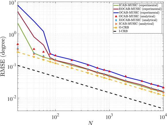
(a)

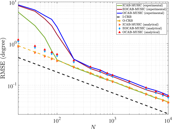
(b)

Figure 2: RMSE in degrees for $\theta_{2}$ versus $N$ for a nested array with $M=10$ elements and configuration given in (58), ${\rm SNR}=3$ dB, and: (a) $K=5<M$; (b) $K=12>M$.

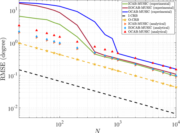
Figure 3: RMSE in degrees for $\theta_{2}$ versus $N$ for a nested array with $M=10$ elements and configuration given in (58) when $K=3$, $\theta_{1}=$$$, $\theta_{2}=$$$, $\theta_{3}=$$$, ${\rm SNR}_{1}=20$ dB, ${\rm SNR}_{2}=8$ dB and ${\rm SNR}_{3}=22$ dB.

VI-B MSE vs. the Number of Snapshots

Fig. 2 depicts the Root-Mean-Squares-Error (RMSE) for $\theta_{2}$ in degree versus the number of snapshots when the nested array in (58) is used. The SNR is assumed to be $3$ dB. In addition, noting $M=10$, two different scenarios are considered: (a) $K=5<M$, and (b) $K=12>M$. Fig. 2 illustrates a close agreement between the numerical simulations and analytical expression derived for RMSEs of OCAB-MUSIC and EOCAB-MUSIC when about $200$ or more snapshots are available. Further, a considerable gap is observed between the performance of OCAB-MUSIC and that of the EOCAB-MUSIC. For instance, at $N=400$, Figs. 2a and 2b show a performance gain of roughly $3$ dB and $1$ dB, respectively, in terms of the RMSE when the EOCAB-MUSIC is used. It is also observed that EOCAB-MUSIC performs as well as ICAB-MUSIC when $K=5<M$. Further, it is observed that the RMSE of EOCAB-MUSIC is very close to O-CRB when $K=5<M$ but we see a gap between them when $K=12>M$.

Fig. 2 also shows that when a small number of snapshots is available, e.g. less than $1000$, all estimators are confronted with substantial performance degradation. This performance loss is justified by the subspace swap arising from the inaccurate estimate of the normalized covariance matrix of $\mathbf{y}(t)$, i.e. $\overline{\mathbf{R}}$, in this case. However, it is seen that the proposed estimator still has superior performance compared to OCAB-MUSIC, even in the low snapshot paradigm.

Fig. 3 depicts the RMSE $\theta_{2}$ in degree versus the number of snapshots when $K=3$ and the sources powers are unequal. Specifically, It is assumed that $\theta_{1}=$$$, $\theta_{2}=$$$, $\theta_{3}=$$$, ${\rm SNR}_{1}=20$ dB, ${\rm SNR}_{2}=8$ dB and ${\rm SNR}_{3}=22$ dB. Comparing Fig. 2 with Fig. 3 reveals that a high difference between the SNRs of the closely-spaced source signals do not have a meaningful impact on the relative asymptotic performance of ICAB-MUSIC, OCAB-MUSIC and EOCAB-MUSIC, however, by increasing the difference between SNRs, OCAB-MUSIC needs more number of snapshots to achieve its asymptotic performance compared to EOCAB-MUSIC and ICAB-MUSIC.

VI-C MSE vs. SNR

Fig. 4 shows the RMSE for $\theta_{2}$ in degrees versus SNR for the same setup used for Fig. 2. The number of snapshots is considered to be $N=500$. It is seen in Figs. 4a and Fig. 4b that the RMSEs of OCAB-MUSIC and EOCAB-MUSIC perfectly match with their asymptotic analytical RMSEs given in Corollary 1 and Corollary 2.

Fig. 4 demonstrates that the I-CRB tends to decay to zero as the SNR increases when $K=5<M$ while it gets saturated as the SNR increases when $K=12>M$. However, as opposed to the I-CRB, O-CRB tends to converge to a constant non-zero value at the high SNR regime for both the cases $K=5<M$ and $K=12>M$. This behavior of O-CRB was already predicted by Theorem 4. In addition, as shown in Theorem 6, the RMSEs of OCAB-MUSIC and EOCAB-MUSIC also converge to a constant non-zero value as the SNR increases for both $K=5<M$ and $K=12>M$.

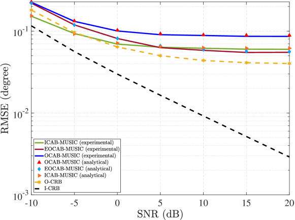
(a)

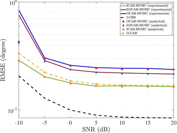
(b)

Figure 4: RMSE in degrees for $\theta_{2}$ versus SNR wen the source powers are equal for a nested array with $M=10$ elements and configuration given in (58), $N=500$, and: (a) $K=5<M$; (b) $K=12>M$.

We observe from Fig. 4 that EOCAB-MUSIC preforms better than OCAB-MUSIC in both scenarios $K=5<M$ and $K=12>M$. For example, at ${\rm SNR}=5$, EOCAB-MUSIC leads to performance gains of about $3.7$ dB and $1.15$ dB in terms of RMSE compared to OCAB-MUSIC. Further, it is seen that EOCAB-MUSIC even outperforms ICAB-MUSIC at high SNR regime when $K=5<M$. Another interesting observation is that the RMSE of O-CRB is either better or equal to that of ICAB-MUSIC.

Fig. 5 shows the RMSE for $\theta_{2}$ in degrees versus SNR when the sources powers are unequal and DoAs are not exactly on the grid as opposed to Fig. 4. The number of snapshots is considered to be $N=500$. In case of $K=5<M$, the sources are located at $\theta_{1}=$$,\theta_{2}=$$,\theta_{3}=$$,\theta_{4}=$$$ and $\theta_{5}=$$$. Further, the source SNRs are assumed to be ${\rm SNR}_{1}=0.75\times{\rm SNR}_{2},{\rm SNR}_{3}=1.22\times{\rm SNR}_{2},{\rm SNR}_{4}=0.92\times{\rm SNR}_{2}$ and ${\rm SNR}_{5}=0.66\times{\rm SNR}_{2}$ while ${\rm SNR}_{2}$ varies from $10$ dB to $20$ dB as shown in Fig. 5a. Further, in case of $K=12>M$, the sources are located at $\theta_{1}=$$,\theta_{2}=$$,\theta_{3}=$$,\theta_{4}=$$,\theta_{5}=$$,\theta_{6}=$$,\theta_{7}=$$,\theta_{8}=$$,\theta_{9}=$$,\theta_{1}0=$$,\theta_{1}1=$$$ and $\theta_{1}2=$$$. The source SNRs are assumed to be ${\rm SNR}_{1}=1.34\times{\rm SNR}_{2},{\rm SNR}_{3}=0.84\times{\rm SNR}_{2},{\rm SNR}_{4}=0.83\times{\rm SNR}_{2},{\rm SNR}_{5}=0.67\times{\rm SNR}_{2},{\rm SNR}_{6}=0.69\times{\rm SNR}_{2},{\rm SNR}_{7}=0.95\times{\rm SNR}_{2},{\rm SNR}_{8}=0.61\times{\rm SNR}_{2},{\rm SNR}_{9}=0.79\times{\rm SNR}_{2},{\rm SNR}_{1}0=0.56\times{\rm SNR}_{2},{\rm SNR}_{1}0=0.82\times{\rm SNR}_{2}$ and ${\rm SNR}_{1}2=0.88\times{\rm SNR}_{2}$ while ${\rm SNR}_{2}$ varies from $10$ dB to $20$ dB as shown in Fig. 5b. Comparing Fig. 5 with Fig. 4 reveals that unequal source powers do not have remarkable impact on the estimation accuracy particularly in high-SNR regime.

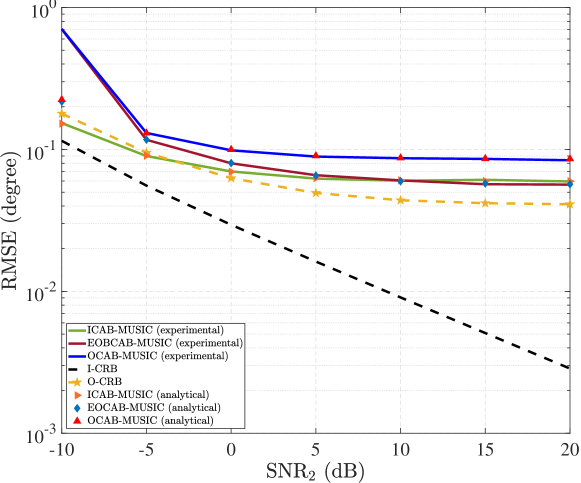
(a)

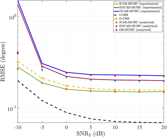
(b)

Figure 5: RMSE in degrees for $\theta_{2}$ versus SNR when the source powers are unequal for a nested array with $M=10$ elements and configuration given in (58), $N=500$, and: (a) $K=5<M$; (b) $K=12>M$.

VI-D CRB vs. the Number of Source Signals

Fig. 6 plots the I-CRB and the O-CRB for $\theta_{2}$ in degree versus the number of source signals for ${\rm SNR}=3\leavevmode\nobreak\ {\rm dB}$ and $N=500$ and different types of arrays given in (58), (59), (60) and (61). The values of $D$ and $v$ for the different types of arrays are as: 1. MRA: $D=37$ and $v=37$; 2. nested array: $D=30$ and $v=30$; 3. co-prime array: $D=26$ and $v=23$; ULA: $D=10$ and $v=10$ . Fig. 6 indicates that both the I-CRB and the O-CRB increase as the number of source signals increases. Moreover, it is observed that the I-CRB and the O-CRB are quite small for all the SLAs as long as $1\leq K\leq v-1$, but they escalate dramatically when $K$ approaches values that are equal to or larger than $D$. This observation is in compliance with Theorem 2 which indicates that the DoA estimation problem is globally identifiable when $1\leq K\leq v-1$ and is globally non-identifiable when $K\geq D$.

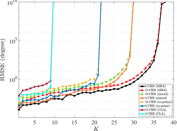
Figure 6: The CRB versus $K$ for various array configurations given from (58) to (60), $N=500$ and ${\rm SNR}=3$ dB.

VI-E Resolution Probability

Fig. 7 depicts the probability of resolution versus the source separation for ICAB-MUSIC, EOCAB-MUSIC and OCAB-MUSIC when the nested array given in (58) is employed. The number of snapshots and the SNR are considered to be $N=500$ and $0$ dB, respectively. In addition, we consider two sources with equal powers, located at $\theta_{1}=$$-\frac{\Delta\theta}{2}$ and $\theta_{2}=$$+\frac{\Delta\theta}{2}$. We define the two sources as being resolvable if ${\rm\underset{\scalebox{0.5}{$i\in\{1,2\}$}}{max}}|\hat{\theta}_{i}-\theta_{i}|<\frac{\Delta\theta}{2}$ [64]. According to this definition and making use of two-dimensional Chebychev’s bound [65], the probability of resolution can be lower bounded as

$$\mathbb{P}({\rm\underset{\scalebox{0.5}{$i\in\{1,2\}$}}{max}}|\hat{\theta}_{i}-\theta_{i}|<\frac{\Delta\theta}{2})$$ (66)

$$=\mathbb{P}(|\hat{\theta}_{1}-\theta_{1}|<\frac{\Delta\theta}{2},|\hat{\theta}_{2}-\theta_{2}|<\frac{\Delta\theta}{2})\geq 1-\frac{2[{\cal E}(\theta_{1})+{\cal E}(\theta_{2})]}{\Delta\theta^{2}}$$

$$+\frac{2\sqrt{{\cal E}^{2}_{\theta_{1}}+{\cal E}^{2}_{\theta_{2}}+2{\cal E}_{\theta_{1}}{\cal E}_{\theta_{2}}-4{\cal E}^{2}_{\theta_{1},\theta_{2}}}}{\Delta\theta^{2}},$$

where ${\cal E}(\theta_{1})$, ${\cal E}(\theta_{2})$ and ${\cal E}(\theta_{1},\theta_{2})$ are given in (54) and (48). The analytical expression on the right-hand side of (66) enables us to predict the minimum source separation required for achieving a particular probability of resolution. For example, Fig. 6 shows the predicted values for the minimum source separation to achieve a probability of resolution greater than $0.9$, obtained from (66), for ICAB-MUSIC, OCAB-MUSIC and EOCAB-MUSIC. It is observed that the predicted values of the minimum source separation for ICAB-MUSIC, EOCAB-MUSIC and OCAB-MUSIC, which are respectively $\Delta\theta=$$$, $\Delta\theta=$$$ and $\Delta\theta=$$$, are in a good agreement with the values obtained from the numerical simulations, which are respectively $\Delta\theta=$$$, $\Delta\theta=$$$ and $\Delta\theta=$$$. Additionally, Fig. 7 demonstrates the resolution performance of EOCAB-MUSIC is superior to that of OCAB-MUSIC while ICAB-MUSIC outperforms both of them.

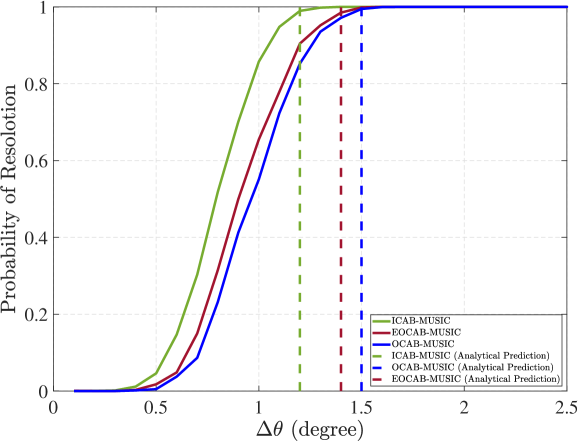
Figure 7: Probability of resolution versus source separation in degree for a nested array with $M=10$ elements and configuration given in (58), $N=500$ and ${\rm SNR}=0$ dB.

VII Conclusion

In this paper, we considered the problem of DoA estimation from one-bit measurements received by an SLA. We showed that the idetifiability condition for the DoA estimation problem from one-bit SLA data is equivalent to that for the case when DoAs are estimated from infinite-bit unquantized measurements. Then, we derived a pessimistic approximation of the corresponding CRB. This pessimistic CRB was used as a benchmark for assessing the performance of one-bit DoA estimators. Further, it provides us with valuable insights on the performance limits of DoA estimation from one-bit quantized data. For example, it was shown that the DoA estimation errors in one-bit scenario reduces at the same rate as that of infinite-bit case with respect to the number of samples and, moreover, that the DoA estimation errors in one-bit scenario converges to a constant value by increasing the SNR. We also proposed a new algorithm for estimating DoAs from one-bit quantized data. We investigated the analytical performance of the proposed method through deriving a closed-form expression for the second-order statistics of its asymptotic distribution (for the large number of snapshots) and show that it outperforms the existing algorithms in the literature. Numerical simulations were provided to validate the analytical derivations and corroborate the improvement in estimation performance.

Appendix A Proof of Theorem 1

We first prove the sufficiency. Assume that $\bm{\theta}_{0}\in[-\pi/2,\pi/2]^{K\times 1}$ is identifiable from $\mathbf{Y}$. This implies that $f(\mathbf{Y}\mid\bm{\theta}_{0},\mathbf{p},\sigma^{2})\neq f(\mathbf{Y}\mid\breve{\bm{\theta}},\breve{\mathbf{p}},\breve{\sigma}^{2})$ for any arbitrary values of $\breve{\bm{\theta}}\neq\bm{\theta}_{0}\in[-\pi/2,\pi/2]^{K\times 1}$, $\mathbf{p}\in\mathds{R}_{>0}^{{K\times 1}}$, $\breve{\mathbf{p}}\in\mathds{R}_{>0}^{{K\times 1}}$, $\sigma^{2}$ and $\breve{\sigma}^{2}$. Hence, considering $\mathbf{y}(0),\mathbf{y}(1),\cdots,\mathbf{y}(N-1)$ are independent and identically distributed with $\mathbf{y}(t)\sim{\cal CN}({\mathbf{0}},\mathbf{R})$, we have

$$\mathbf{A}\!(\bm{\theta}_{0}){\mathrm{diag}}(\mathbf{p})\mathbf{A}\!^{H}\!(\bm{\theta}_{0})\!+\!\sigma^{2}{\mathbf{I}}_{M}\!\neq\!\mathbf{A}\!(\breve{\bm{\theta}}){\mathrm{diag}}(\breve{\mathbf{p}})\mathbf{A}\!^{H}\!(\breve{\bm{\theta}})\!+\!\breve{\sigma}^{2}{\mathbf{I}}_{M},$$ (67)

for all $\breve{\bm{\theta}}\neq\bm{\theta}_{0}\in[-\pi/2,\pi/2]^{K\times 1}$, $\mathbf{p}\in\mathds{R}_{>0}^{{K\times 1}}$, $\breve{\mathbf{p}}\in\mathds{R}_{>0}^{{K\times 1}}$, $\sigma^{2}$ and $\breve{\sigma}^{2}$.

In what follows, we employ the method of proof by contradiction to prove the sufficiency. In particular, we assume that $\bm{\theta}_{0}\in[-\pi/2,\pi/2]^{K\times 1}$ is non-identifiable from $\mathbf{X}$. Hence, there exists a $\breve{\bm{\theta}}\neq\bm{\theta}_{0}\in[-\pi/2,\pi/2]^{K\times 1}$ at which $f(\mathbf{X}\mid\bm{\theta}_{0},\widetilde{\mathbf{p}},\widetilde{\sigma}^{2})=f(\mathbf{X}\mid\breve{\bm{\theta}},\dot{\mathbf{p}},\dot{\sigma}^{2})$ for some values of $\widetilde{\mathbf{p}}\in\mathds{R}_{>0}^{{K\times 1}}$, $\dot{\mathbf{p}}\in\mathds{R}_{>0}^{{K\times 1}}$, $\widetilde{\sigma}^{2}$ and $\dot{\sigma}^{2}$. It is readily clear from assumption A4 and (6) that ${\mathbb{E}}\{\mathbf{x}(t_{1})\mathbf{x}^{H}(t_{2})\}={\mathbf{0}}$ when $t_{1}\neq t_{2}$. Accordingly, we have

$${\mathbb{E}}\left\{\mathbf{X}\mathbf{X}^{H}\!\mid\!\bm{\theta}_{0},\widetilde{\mathbf{p}},\widetilde{\sigma}^{2}\right\}={\mathbb{E}}\left\{\mathbf{X}\mathbf{X}^{H}\!\mid\!\breve{\bm{\theta}},\dot{\mathbf{p}},\dot{\sigma}^{2}\right\},$$ (68)

$$\Rightarrow \!\sum_{t=0}^{N-1}{\mathbb{E}}\{\mathbf{x}(t)\mathbf{x}^{H}(t)\!\mid\!\bm{\theta}_{0},\widetilde{\mathbf{p}},\widetilde{\sigma}^{2}\}\!=\!\sum_{t=0}^{N-1}{\mathbb{E}}\{\mathbf{x}(t)\mathbf{x}^{H}(t)\!\mid\!\breve{\bm{\theta}},\dot{\mathbf{p}},\dot{\sigma}^{2}\}.$$

From (68), (7), (3) and the fact that the arcsine function is one-to-one when its argument is between $-1$ and $1$, it follows that

$$\frac{1}{\widetilde{\sigma}^{2}+\sum_{k=1}^{K}\tilde{p}_{k}}\left[\mathbf{A}(\bm{\theta}_{0}){\mathrm{diag}}(\widetilde{\mathbf{p}})\mathbf{A}^{H}(\bm{\theta}_{0})\!+\!\widetilde{\sigma}^{2}{\mathbf{I}}_{M}\right]=$$

$$\frac{1}{\dot{\sigma}^{2}+\sum_{k=1}^{K}\dot{p}_{k}}\left[\mathbf{A}(\breve{\bm{\theta}}){\mathrm{diag}}(\dot{\mathbf{p}})\mathbf{A}^{H}(\breve{\bm{\theta}})\!+\!\dot{\sigma}^{2}{\mathbf{I}}_{M}\right].$$ (69)

Considering $\mathbf{p}=\frac{\widetilde{\mathbf{p}}}{\widetilde{\sigma}^{2}+\sum_{k=1}^{K}\tilde{p}_{k}}$, $\sigma^{2}=\frac{\widetilde{\sigma}^{2}}{\widetilde{\sigma}^{2}+\sum_{k=1}^{K}\tilde{p}_{k}}$, $\breve{\mathbf{p}}=\frac{\dot{\mathbf{p}}}{\dot{\sigma}^{2}+\sum_{k=1}^{K}\dot{p}_{k}}$ and $\breve{\sigma}^{2}=\frac{\dot{\sigma}^{2}}{\dot{\sigma}^{2}+\sum_{k=1}^{K}\dot{p}_{k}}$, we obtain

$$\mathbf{A}(\bm{\theta}_{0}){\mathrm{diag}}(\mathbf{p})\mathbf{A}^{H}(\bm{\theta}_{0})+\sigma^{2}{\mathbf{I}}_{M}=\mathbf{A}\!(\breve{\bm{\theta}}){\mathrm{diag}}(\breve{\mathbf{p}})\mathbf{A}^{H}(\breve{\bm{\theta}})+\breve{\sigma}^{2}{\mathbf{I}}_{M},$$ (70)

which is in contradiction with (67). Hence, the initial assumption that $\bm{\theta}_{0}\in[-\pi/2,\pi/2]^{K\times 1}$ is non-identifiable from $\mathbf{X}$ cannot be true. This proves the sufficiency.

To show the necessity, let assume that $\bm{\theta}_{0}\in[-\pi/2,\pi/2]^{K\times 1}$ is non-identifiable from $\mathbf{Y}$. This implies that there exist some $\breve{\bm{\theta}}\in[-\pi,\pi]^{q\times 1}\neq\bm{\theta}_{0}$, $\mathbf{p}$, $\breve{\mathbf{p}}$, $\sigma^{2}$ and $\breve{\sigma}^{2}$ for which $f(\mathbf{Y}\mid\bm{\theta}_{0},\mathbf{p},\sigma^{2})=f(\mathbf{Y}\mid\breve{\bm{\theta}},\breve{\mathbf{p}},\breve{\sigma}^{2})$. Since the true PDF of $\mathbf{X}$ is obtained from the orthant probabilities of $\mathbf{Y}$, it is readily deduced that $f(\mathbf{X}\mid\bm{\theta}_{0},\mathbf{p},\sigma^{2})=f(\mathbf{X}\mid\breve{\bm{\theta}},\breve{\mathbf{p}},\breve{\sigma}^{2})$ as well. This proves that identifiability of $\bm{\theta}_{0}\in[-\pi/2,\pi/2]^{K\times 1}$ from $\mathbf{Y}$ is a necessary condition for identifiability of $\bm{\theta}_{0}\in[-\pi/2,\pi/2]^{K\times 1}$ from $\mathbf{X}$.

Appendix B Proof of Theorem 2

We first prove S1. Consider arbitrary $\bm{\theta}\neq\in[-\pi/2,\pi/2]^{K\times 1}$ and $\breve{\bm{\theta}}\in[-\pi/2,\pi/2]^{K\times 1}$ such that $\bm{\theta}_{k}\neq\breve{\bm{\theta}}$. Moreover, let $\mathbf{A}_{v}(\bm{\theta})$ be the steering matrix of a contiguous ULA with $v$ elements located at $(0,\frac{\lambda}{2},\cdots,(v-1)\frac{\lambda}{2})$. Considering the fact that $\mathbf{A}_{v}(\bm{\theta})$ is a Vandermonde matrix, if $K\leq v-1$, it follows from Caratheodory-Fejer-Pisarenko decomposition [66] that

$$\mathbf{A}_{v}(\bm{\theta}){\mathrm{diag}}(\mathbf{p})\mathbf{A}_{v}^{H}\!(\bm{\theta})\!+\!\sigma^{2}{\mathbf{I}}_{v}\!\neq\!\mathbf{A}_{v}\!(\breve{\bm{\theta}}){\mathrm{diag}}(\breve{\mathbf{p}})\mathbf{A}_{v}^{H}\!(\breve{\bm{\theta}})\!+\!\breve{\sigma}^{2}{\mathbf{I}}_{v},$$ (71)

for any arbitrary values of $\mathbf{p}\in\mathds{R}_{>0}^{{K\times 1}}$, $\breve{\mathbf{p}}\in\mathds{R}_{>0}^{{K\times 1}}$, $\sigma^{2}$ and $\breve{\sigma}^{2}$. From [23, Eq. (113)], vectorizing both sides of (71) leads to

$$\mathbf{T}{{}^{\prime}}\mathbf{A}_{\vartheta}(\bm{\theta})\mathbf{p}+\sigma^{2}\mathbf{T}{{}^{\prime}}\mathbf{e}{{}^{\prime}}\neq\mathbf{T}{{}^{\prime}}\mathbf{A}_{\vartheta}(\breve{\bm{\theta}})\breve{\mathbf{p}}+\breve{\sigma}^{2}\mathbf{T}{{}^{\prime}}\mathbf{e}{{}^{\prime}},$$ (72)

where $\mathbf{A}_{\vartheta}(\bm{\theta})\in\mathds{C}^{(2v-1)\times K}$ denotes the steering matrix corresponding to the contiguous ULA segment of the difference co-array, $\mathbf{T}^{\prime}\in\{0,1\}^{v^{2}\times(2v-1)}$ is a selection matrix defined in [23, Eq. (114)] and $\mathbf{e}{{}^{\prime}}\in\{0,1\}^{(2v-1)\times 1}$ is a column vector with $[\mathbf{e}{{}^{\prime}}]_{i}=\delta[i-v]$. Considering $\mathbf{T}^{\prime}$ is full-column rank [23], multiplying both sides of (72) by $\mathbf{T}^{\prime\dagger}$ and then moving all the terms to one side of the equation yields

$$\mathbf{A}_{\vartheta}(\bm{\theta})\mathbf{p}-\mathbf{A}_{\vartheta}(\breve{\bm{\theta}})\breve{\mathbf{p}}+(\sigma^{2}-\breve{\sigma}^{2})\mathbf{e}{{}^{\prime}}\neq{\mathbf{0}}.$$ (73)

It follows from $\breve{\bm{\theta}}\!\neq\!\bm{\theta}_{0}$ that $\breve{\bm{\theta}}$ could differs from $\bm{\theta}_{0}$ at $q$ DoAs for some integer $q\!\in\![1,K]$. Noting this fact, (73) is simplified to

$$\begin{bmatrix}\mathbf{A}_{\vartheta}(\bm{\theta})&\mathbf{A}_{\vartheta}(\ddot{\bm{\theta}})&\mathbf{e}{{}^{\prime}}\end{bmatrix}\begin{bmatrix}\mathbf{p}-\breve{\mathbf{p}}\odot\bm{\varepsilon}\\ -\ddot{\mathbf{p}}\\ \sigma^{2}-\breve{\sigma}^{2}\end{bmatrix}\neq{\mathbf{0}},$$ (74)

where $\ddot{\bm{\theta}}\in[-\pi,\pi]^{q\times 1}$ consists of those elements of $\breve{\bm{\theta}}$ which do not intersect with those in $\bm{\theta}$, $\ddot{\mathbf{p}}\in\mathds{R}_{>0}^{q\times 1}$ contains those elements of $\breve{\mathbf{p}}$ corresponding to $\ddot{\bm{\theta}}$ and

$$[\bm{\varepsilon}]_{i}=\left\{\begin{array}[]{cc}1,&[\bm{\theta}]_{i}=[\breve{\bm{\theta}}]_{i},\\ 0,&\text{otherwise}.\end{array}\right.$$ (77)

Considering that $\begin{bmatrix}\mathbf{A}_{\vartheta}(\bm{\theta})\!&\!\mathbf{A}_{\vartheta}(\breve{\bm{\theta}})\!&\!\mathbf{e}^{{}^{\prime}}\end{bmatrix}\in\mathds{C}^{(2v-1)\times(2K+1)}$  is a sub-matrix of $\begin{bmatrix}\mathbf{A}_{d}(\bm{\theta})\!&\!\mathbf{A}_{d}(\ddot{\bm{\theta}})\!&\!\mathbf{e}\end{bmatrix}\in\mathds{C}^{(2D-1)\times(2K+1)}$, obtained from $2v-1$ rows of $\begin{bmatrix}\mathbf{A}_{d}(\bm{\theta})\!&\!\mathbf{A}_{d}(\ddot{\bm{\theta}})\!&\!\mathbf{e}\end{bmatrix}$, it follows from (74) that

$$\begin{bmatrix}\mathbf{A}_{d}(\bm{\theta})&\mathbf{A}_{d}(\ddot{\bm{\theta}})&\mathbf{e}\end{bmatrix}\begin{bmatrix}\mathbf{p}-\breve{\mathbf{p}}\odot\bm{\varepsilon}\\ -\ddot{\mathbf{p}}\\ \sigma^{2}-\breve{\sigma}^{2}\end{bmatrix}\neq{\mathbf{0}},$$ (78)

$$\Rightarrow \mathbf{A}_{d}(\bm{\theta})\mathbf{p}-\mathbf{A}_{d}(\breve{\bm{\theta}})\breve{\mathbf{p}}+(\sigma^{2}-\breve{\sigma}^{2})\mathbf{e}\neq{\mathbf{0}}.$$ (79)

Multiplying (79) by $\mathbf{J}$ and exploiting (3) and (II), after some algebraic manipulations, we obtain

$${\mathrm{vec}}(\mathbf{A}(\bm{\theta}){\mathrm{diag}}(\mathbf{p})\mathbf{A}^{H}(\bm{\theta})+\sigma^{2}{\mathbf{I}}_{M})$$

$$\neq{\mathrm{vec}}(\mathbf{A}(\breve{\bm{\theta}}){\mathrm{diag}}(\breve{\mathbf{p}})\mathbf{A}^{H}(\breve{\bm{\theta}})+\breve{\sigma}^{2}{\mathbf{I}}_{M}),$$ (80)

which in turn implies that

$$\mathbf{A}\!(\bm{\theta}){\mathrm{diag}}(\mathbf{p})\mathbf{A}^{H}\!(\bm{\theta})\!+\!\sigma^{2}{\mathbf{I}}_{M}\!\neq\!\mathbf{A}\!(\breve{\bm{\theta}}){\mathrm{diag}}(\breve{\mathbf{p}})\mathbf{A}^{H}\!(\breve{\bm{\theta}})\!+\!\breve{\sigma}^{2}{\mathbf{I}}_{M},$$ (81)

for all $\bm{\theta}\neq\breve{\bm{\theta}}\in[-\pi/2,\pi/2]^{K\times 1}$, $\mathbf{p}\in\mathds{R}_{>0}^{{K\times 1}}$, $\breve{\mathbf{p}}\in\mathds{R}_{>0}^{{K\times 1}}$, $\sigma^{2}$ and $\breve{\sigma}^{2}$. Considering $\mathbf{y}(0),\mathbf{y}(1),\cdots,\mathbf{y}(N-1)$ are independent and identically distributed with $\mathbf{y}(t)\sim{\cal CN}({\mathbf{0}},\mathbf{R})$, it follows from (81) that $f(\mathbf{Y}\mid\bm{\theta}_{0},\mathbf{p},\sigma^{2})\neq f(\mathbf{Y}\mid\breve{\bm{\theta}},\breve{\mathbf{p}},\breve{\sigma}^{2})$ for any arbitrary values of $\bm{\theta}\neq\breve{\bm{\theta}}\in[-\pi/2,\pi/2]^{K\times 1}$, $\mathbf{p}\in\mathds{R}_{>0}^{{K\times 1}}$, $\breve{\mathbf{p}}\in\mathds{R}_{>0}^{{K\times 1}}$, $\sigma^{2}$ and $\breve{\sigma}^{2}$ if $K\leq v-1$. Now, from Theorem 1, we conclude that $f(\mathbf{X}\mid\bm{\theta}_{0},\mathbf{p},\sigma^{2})\neq f(\mathbf{X}\mid\breve{\bm{\theta}},\breve{\mathbf{p}},\breve{\sigma}^{2})$. This completes the proof of S1.

We now prove S2. We know from Lemma 1 that the FIM is singular for any value of $\bm{\theta}\in[-\pi/2,\pi/2]^{K\times 1}$ if $K\geq D$. This means that the problem is not even locally indentifiable at any $\bm{\theta}$ [67]. Since the local identifiablity is a necessary condition for the identifiablity any particular point, the problem is not identifiable for any $\bm{\theta}$.

Appendix C Proof of Lemma 1

Let $\mathbf{R}_{\mathbf{x}}^{r}$ and $\overline{\mathbf{R}}^{r}$ denote the equivalent real representation for $\mathbf{R}_{\mathbf{x}}$ and $\overline{\mathbf{R}}$, respectively, given as

$$\mathbf{R}_{\mathbf{x}}^{r}=\begin{bmatrix}\Re\{\mathbf{R}_{\mathbf{x}}\}&-\Im\{\mathbf{R}_{\mathbf{x}}\}\\ \Im\{\mathbf{R}_{\mathbf{x}}\}&\Re\{\mathbf{R}_{\mathbf{x}}\}\end{bmatrix},\leavevmode\nobreak\ \leavevmode\nobreak\ \overline{\mathbf{R}}^{r}=\begin{bmatrix}\Re\{\overline{\mathbf{R}}\}&-\Im\{\overline{\mathbf{R}}\}\\ \Im\{\overline{\mathbf{R}}\}&\Re\{\overline{\mathbf{R}}\}.\end{bmatrix}$$ (82)

Making use of (7) and Taylor expansion of arcsine function, we have

$$\mathbf{R}_{\mathbf{x}}^{r}= \frac{2}{\pi}\arcsin(\overline{\mathbf{R}}^{r})=\overline{\mathbf{R}}^{r}+\frac{1}{6}\overline{\mathbf{R}}^{r}\odot\overline{\mathbf{R}}^{r}\odot\overline{\mathbf{R}}^{r}$$

$$+\frac{3}{40}\overline{\mathbf{R}}^{r}\odot\overline{\mathbf{R}}^{r}\odot\overline{\mathbf{R}}^{r}\odot\overline{\mathbf{R}}^{r}\odot\overline{\mathbf{R}}^{r}+\cdots$$

$$= \sum_{n=0}^{\infty}\frac{(2n)!}{(2^{n}n!)^{2}(2n+1)}\underbrace{\overline{\mathbf{R}}^{r}\odot\overline{\mathbf{R}}^{r}\odot\cdots\odot\overline{\mathbf{R}}^{r}}_{2n+1\leavevmode\nobreak\ {\rm times}}.$$ (83)

It is clear from (8) that $\overline{\mathbf{R}}$ is positive definite, and so is $\overline{\mathbf{R}}^{r}$. Further, it follows from the Schur product theorem [68, Theorem 3.1], which establishes that the Hadamard product of two positive-definite matrices is also a positive-definite matrix, that the $2n+1$ times Hadamard products of $\overline{\mathbf{R}}^{r}$ by itself is also positive definite for any integer $n\in[0,\infty)$. Hence, it follows from (C) that $\mathbf{R}_{\mathbf{x}}^{r}$ is obtained from a weighted sum of positive definite matrices, and thus it is positive definite. Evidently, $\mathbf{R}_{\mathbf{x}}$ is also positive definite. This in turn indicates non-singularity of $(\mathbf{R}_{\mathbf{x}}^{-T}\otimes\mathbf{R}_{\mathbf{x}}^{-1})$. Hence, since $\mathbf{J}$ is also full-column rank [13], we easily conclude that $\mathbf{J}^{H}(\mathbf{R}_{\mathbf{x}}^{-T}\otimes\mathbf{R}_{\mathbf{x}}^{-1})\mathbf{J}$ is full rank. This implies that ${\cal I}_{w}(\bm{\varrho})$ is non-singular if and only if $\begin{bmatrix}\mathbf{G}&\mathbf{V}\end{bmatrix}\in\mathds{R}^{(2D-1)\times 2K}$is full-column rank. In other words, ${\cal I}_{w}(\bm{\varrho})$ is non-singular if and only if

$$\begin{bmatrix}\mathbf{G}&\mathbf{V}\end{bmatrix}\begin{bmatrix}\mathbf{c}_{1}\\ \mathbf{c}_{2}\end{bmatrix}\neq{\mathbf{0}},$$ (84)

for any arbitrary non-zero $\mathbf{c}=[\mathbf{c}_{1}^{T},\mathbf{c}_{2}^{T}]^{T}\in\mathds{C}^{2K\times 1}$. Inserting (16) and (17) into (84) leads to

$$\begin{bmatrix}\mathbf{\Delta}&\mathbf{\digamma}\end{bmatrix}\begin{bmatrix}\widetilde{\mathbf{c}}_{1}\\ \mathbf{c}_{2}\end{bmatrix}\neq{\mathbf{0}},$$ (85)

where $\widetilde{\mathbf{c}}_{1}\!=\!j\pi\bm{\Phi}(\bm{\theta}){\mathrm{diag}}(\overline{\mathbf{p}})\mathbf{c}_{1}$. This completes the proof.

Appendix D Proof of Theorem 3

We know from Appendix C that $\mathbf{M}=\mathbf{J}^{H}(\mathbf{R}_{\mathbf{x}}^{-T}\otimes\mathbf{R}_{\mathbf{x}}^{-1})\mathbf{J}$ is positive-definite. Hence, (15) can be rewritten as

$${\cal I}_{w}(\bm{\varrho}) =N\begin{bmatrix}\mathbf{G}^{H}\mathbf{M}^{\frac{1}{2}}\\ \mathbf{V}^{H}\mathbf{M}^{\frac{1}{2}}\end{bmatrix}\begin{bmatrix}\mathbf{M}^{\frac{1}{2}}\mathbf{G}&\mathbf{M}^{\frac{1}{2}}\mathbf{V}\end{bmatrix}$$

$$=N\begin{bmatrix}\mathbf{G}^{H}\mathbf{M}\mathbf{G}&\mathbf{G}^{H}\mathbf{M}\mathbf{V}\\ \mathbf{V}^{H}\mathbf{M}\mathbf{G}&\mathbf{V}^{H}\mathbf{M}\mathbf{V}\end{bmatrix}.$$ (86)

The $CRB_{w}(\bm{\theta})$ is then obtained by block-wise inversion as follows:

$$CRB_{w}(\bm{\theta}) \!=\!\frac{1}{N}\left(\mathbf{G}^{H}\mathbf{M}\mathbf{G}\!-\!\mathbf{G}^{H}\mathbf{M}\mathbf{V}\left(\mathbf{V}^{H}\mathbf{M}\mathbf{V}\right)^{-1}\mathbf{V}^{H}\mathbf{M}\mathbf{G}\right)^{-1}$$

$$\!=\!\frac{1}{N}\left(\mathbf{G}^{H}\mathbf{M}^{\frac{1}{2}}\Pi^{\perp}_{\mathbf{M}^{\frac{1}{2}}\mathbf{V}}\mathbf{M}^{\frac{1}{2}}\mathbf{G}\right)^{-1}.$$ (87)

The facts that $\mathbf{G}=j\pi{\mathrm{diag}}(\mathbf{d})\mathbf{\Omega}\mathbf{\Phi}(\bm{\theta}){\mathrm{diag}}(\overline{\mathbf{p}})$ and $\mathbf{R}_{\mathbf{x}}=\frac{2}{\pi}{\mathrm{arcsine}}(\overline{\mathbf{R}})$ will lead to (20). In addition, It follows from ${\cal I}(\varrho)\succeq{\cal I}_{w}(\bm{\varrho})$ that $CRB(\bm{\theta})\preceq CRB_{w}(\bm{\theta})$.

Appendix E Proof of Theorem 4

Recalling $\overline{p}_{k}=\frac{p_{k}}{\sigma^{2}+\sum_{k=1}^{K}p_{k}}$ and assuming that all sources have equal power $p$, we have

$$\lim_{SNR\to\infty}\overline{p}_{k}=\lim_{SNR\to\infty}\frac{SNR}{K\times SNR+1}=\frac{1}{K}.$$ (88)

Making use of (88), it can be readily shown that

$$\lim_{SNR\to\infty}\overline{\mathbf{R}} =\frac{1}{K}\mathbf{A}(\bm{\theta})\mathbf{A}^{H}(\bm{\theta})+(1-\frac{1}{K}){\mathbf{I}}_{M}.$$ (89)

The above equation implies that $\lim_{SNR\to\infty}\overline{\mathbf{R}}$ is a positive-definite matrix independent of the SNR. Further, it follows from (88) that

$$\lim_{SNR\to\infty}{\mathrm{diag}}(\overline{\mathbf{p}})=\frac{1}{K}{\mathbf{I}}_{K},$$ (90)

$$\lim_{SNR\to\infty}\mathbf{h}=\bigg{[}\frac{1}{\sqrt{1-\frac{|\Re\{\sum_{k=1}^{K}e^{-j\pi\sin\theta_{k}\ell_{D-1}}\}|^{2}}{K^{2}}}},\cdots,0,$$

$$\leavevmode\nobreak\ \leavevmode\nobreak\ \leavevmode\nobreak\ \leavevmode\nobreak\ \leavevmode\nobreak\ \cdots,\frac{1}{\sqrt{1-\frac{|\Re\{\sum_{k=1}^{K}e^{j\pi\sin\theta_{k}\ell_{D-1}}\}|^{2}}{K^{2}}}}\bigg{]}^{T},$$ (91)

$$\lim_{SNR\to\infty}\overline{\mathbf{h}}=\bigg{[}\frac{1}{\sqrt{1-\frac{|\Im\{\sum_{k=1}^{K}e^{-j\pi\sin\theta_{k}\ell_{D-1}}\}|^{2}}{K^{2}}}},\cdots,0,$$

$$\leavevmode\nobreak\ \leavevmode\nobreak\ \leavevmode\nobreak\ \leavevmode\nobreak\ \leavevmode\nobreak\ \cdots,\frac{1}{\sqrt{1-\frac{|\Im\{\sum_{k=1}^{K}e^{j\pi\sin\theta_{k}\ell_{D-1}}\}|^{2}}{K^{2}}}}\bigg{]}^{T}.$$ (92)

Substituting (90), (E) and (E) back into (16) and (17) indicates that $\lim_{SNR\to\infty}\begin{bmatrix}\mathbf{G}&\mathbf{V}\end{bmatrix}$ is a full-column rank matrix independent of the SNR. Hence, recalling (15), we can conclude that $\lim_{SNR\to\infty}{\cal I}_{w}(\varrho)$ is positive-definite and independent of the SNR. This in turn implies that $\lim_{SNR\to\infty}CRB_{w}(\bm{\theta})$, which is Schur complement of $\lim_{SNR\to\infty}{\cal I}_{w}(\varrho)$, is also positive-definite and independent of the SNR. This completes the proof.

Appendix F Proof of Lemma 2

We start with showing that $\mathbf{\Psi}$ is full rank. Making use of relations $\det(\begin{bmatrix}\mathbf{C}_{1}&\mathbf{C}_{2}\\ \mathbf{C}_{3}&\mathbf{C}_{4}\end{bmatrix})=\det(\mathbf{C}_{1})\det(\mathbf{C}_{4}-\mathbf{C}_{3}\mathbf{C}_{1}^{-1}\mathbf{C}_{2})$, we obtain

$$\det(\mathbf{\Psi})=\det({\mathbf{I}}_{D-1})\det(2j{\mathbf{I}}_{D-1})=(2j)^{D-1}\neq 0,$$ (93)

which implies full rankness of $\mathbf{\Psi}$.

Next, we proceed with proving that $\overline{\mathbf{J}}$ is full rank. Let $\ddot{\mathbf{J}}$ denote the matrix obtained after removing the $D$-th column from $\mathbf{J}$. $\ddot{\mathbf{J}}$ is full column rank since its columns are a sub-set of the columns of the full-column-rank matrix $\mathbf{J}$ [13]. Further, for $1\leq i\leq M$, it is readily confirmed that the $((i-1)M+1)$-th row of ${\mathrm{vec}}(\mathbf{L}_{n})$ as well as ${\mathrm{vec}}(\mathbf{L}_{n}^{T})$ equals the $i$-th diagonal element of $\mathbf{L}_{n}$, which is obviously zero for $n\neq 0$ according to the definition given after (5). Given (5), this in turn implies that the rows of $\ddot{\mathbf{J}}$ with indices $(i-1)M+1$, for all $1\leq i\leq M$, are zero vectors. As a result, the matrix obtained by removing these rows from $\ddot{\mathbf{J}}$, i.e., $\overline{\mathbf{J}}$, has the same column rank as $\ddot{\mathbf{J}}$. This completes the proof.

Finally, we show that $\mathbf{F}$ is full rank. It follows from the fact that $\overline{\mathbf{e}}_{p}^{T}\overline{\mathbf{e}}_{q}=0$ for $p\neq q$ that

$$(\overline{\mathbf{e}}_{i}^{T}\otimes\overline{\mathbf{e}}_{j}^{T}\pm\overline{\mathbf{e}}_{j}^{T}\otimes\overline{\mathbf{e}}_{i}^{T})(\overline{\mathbf{e}}_{p}\otimes\overline{\mathbf{e}}_{q}\pm\overline{\mathbf{e}}_{q}\otimes\overline{\mathbf{e}}_{p})=\overline{\mathbf{e}}_{i}^{T}\overline{\mathbf{e}}_{p}\otimes\overline{\mathbf{e}}_{j}^{T}\overline{\mathbf{e}}_{q}$$

$$\pm\overline{\mathbf{e}}_{i}^{T}\overline{\mathbf{e}}_{q}\otimes\overline{\mathbf{e}}_{j}^{T}\overline{\mathbf{e}}_{p}\pm\overline{\mathbf{e}}_{j}^{T}\overline{\mathbf{e}}_{p}\otimes\overline{\mathbf{e}}_{i}^{T}\overline{\mathbf{e}}_{q}\pm\overline{\mathbf{e}}_{j}^{T}\overline{\mathbf{e}}_{q}\otimes\overline{\mathbf{e}}_{i}^{T}\overline{\mathbf{e}}_{p}=0.$$ (94)

for $1\leq i<j\leq M$ and $1\leq p<q\leq M$ when either $p$ or $q$ differs from $i$ and $j$. In addition, in case $i=p$ and $j=q$, we have

$$(\overline{\mathbf{e}}_{i}^{T}\otimes\overline{\mathbf{e}}_{j}^{T}+\overline{\mathbf{e}}_{j}^{T}\otimes\overline{\mathbf{e}}_{i}^{T})(\overline{\mathbf{e}}_{i}\otimes\overline{\mathbf{e}}_{j}-\overline{\mathbf{e}}_{j}\otimes\overline{\mathbf{e}}_{i})=\overline{\mathbf{e}}_{i}^{T}\overline{\mathbf{e}}_{i}\otimes\overline{\mathbf{e}}_{j}^{T}\overline{\mathbf{e}}_{j}$$

$$-\overline{\mathbf{e}}_{i}^{T}\overline{\mathbf{e}}_{j}\otimes\overline{\mathbf{e}}_{j}^{T}\overline{\mathbf{e}}_{i}+\overline{\mathbf{e}}_{j}^{T}\overline{\mathbf{e}}_{i}\otimes\overline{\mathbf{e}}_{i}^{T}\overline{\mathbf{e}}_{j}-\overline{\mathbf{e}}_{j}^{T}\overline{\mathbf{e}}_{j}\otimes\overline{\mathbf{e}}_{i}^{T}\overline{\mathbf{e}}_{i}=0.$$ (95)

It is also observed that, for $1\leq i\leq M$ and $1\leq p<q\leq M$, the $((i-1)M+1)$-th element of $\overline{\mathbf{e}}_{p}^{T}\otimes\overline{\mathbf{e}}_{q}^{T}\pm\overline{\mathbf{e}}_{p}^{T}\otimes\overline{\mathbf{e}}_{q}^{T}$ is equal to the $i$-th diagonal element of $\overline{\mathbf{e}}_{p}\overline{\mathbf{e}}_{q}^{T}\pm\overline{\mathbf{e}}_{p}\overline{\mathbf{e}}_{q}^{T}$, which is obviously zero for $p\neq q$. Consequently, the row vectors obtained by removing the elements with indices $(i-1)M+1$ for all $1\leq i\leq M$ from $\overline{\mathbf{e}}_{p}^{T}\otimes\overline{\mathbf{e}}_{q}^{T}+\overline{\mathbf{e}}_{q}^{T}\otimes\overline{\mathbf{e}}_{p}^{T}$ and $\overline{\mathbf{e}}_{p}^{T}\otimes\overline{\mathbf{e}}_{q}^{T}-\overline{\mathbf{e}}_{q}^{T}\otimes\overline{\mathbf{e}}_{p}^{T}$ will be still orthogonal with each other. Hence, it is deduced that the square matrix $\mathbf{F}$ has orthogonal rows, thereby being full rank.

Appendix G Proof of Lemma 3

Let define $E(\theta)=\mathbf{a}_{v}^{H}(\theta)\widehat{\mathbf{U}}_{n}\widehat{\mathbf{U}}^{H}_{n}\mathbf{a}_{v}(\theta)$ and $\breve{E}(\theta)=\mathbf{a}_{v}^{H}(\bm{\theta})\mathbf{U}_{n}\mathbf{U}^{H}_{n}\mathbf{a}_{v}(\bm{\theta})$ where $\widehat{\mathbf{U}}_{n}$ and $\mathbf{U}_{n}$ consist of, respectively, the eigenvectors of $\widehat{\overline{\mathbf{R}}}_{v}$ and $\mathbf{A}_{v}(\bm{\theta}){\mathrm{diag}}(\overline{\mathbf{p}})\mathbf{A}_{v}^{H}(\bm{\theta})+\overline{\sigma}^{2}{\mathbf{I}}_{v}$ corresponding to their $v-K$ smallest eigenvalues with $K\leq v-1$. We know that the elements of $\widehat{\bm{\theta}}$ are equal to the minimizers of $E(\theta)$. Defining $E_{n}={\underset{\theta}{\rm sup}}|E(\theta)-\breve{E}(\theta)|$, we have

$$E_{n} ={\underset{\theta}{\rm sup}}\left|\mathbf{a}_{v}^{H}(\bm{\theta})(\widehat{\mathbf{U}}_{n}\widehat{\mathbf{U}}^{H}_{n}-\mathbf{U}_{n}\mathbf{U}^{H}_{n})\mathbf{a}_{v}(\bm{\theta})\right|$$

$$={\underset{\theta}{\rm sup}}\left|\left(\mathbf{a}_{v}^{T}(\bm{\theta})\otimes\mathbf{a}_{v}^{H}(\bm{\theta})\right){\mathrm{vec}}(\widehat{\mathbf{U}}_{n}\widehat{\mathbf{U}}^{H}_{n}-\mathbf{U}_{n}\mathbf{U}^{H}_{n})\right|$$

$$\leq\|\mathbf{a}_{v}^{T}(\bm{\theta})\otimes\mathbf{a}_{v}^{H}(\bm{\theta})\|_{2}\|{\mathrm{vec}}(\widehat{\mathbf{U}}_{n}\widehat{\mathbf{U}}^{H}_{n}-\mathbf{U}_{n}\mathbf{U}^{H}_{n})\|_{2}$$

$$=v^{2}\|{\mathrm{vec}}(\widehat{\mathbf{U}}_{n}\widehat{\mathbf{U}}^{H}_{n}-\mathbf{U}_{n}\mathbf{U}^{H}_{n})\|_{2}.$$ (96)

It follows from (V-A) that $\lim_{N\to\infty}\widehat{\mathbf{U}}_{n}\widehat{\mathbf{U}}^{H}_{n}=\mathbf{U}_{n}\mathbf{U}^{H}_{n}$. Hence, $E_{n}\to 0$ as $N\to\infty$. This implies that $E(\theta)$ converges uniformly to $\breve{E}(\theta)$ as $N\to\infty$. Thus, the minimizers of $E(\theta)$, i.e., the elements of $\widehat{\bm{\theta}}$, converge to the minimizers of $\breve{E}(\theta)$, i.e., $\theta_{1},\theta_{2},\cdots,\theta_{K}$, as $N\to\infty$. This completes the proof.

Appendix H Proof of Theorem 5

Considering the consistency of $\widehat{\bm{\theta}}$ and following the same arguments as in [21, App. B], for sufficiently large $N$, the asymptotic estimation error expression for EOCAB-MUSIC is given by

$$\hat{\theta}_{k}-\theta_{k}=-\frac{\Re\{\mathbf{z}^{T}_{k}\mathbf{T}\mathbf{J}^{\dagger}\Delta\overline{\mathbf{r}}\}}{\pi\overline{p}_{k}q_{k}\cos(\theta_{k})},$$ (97)

where $\Delta\overline{\mathbf{r}}=\widehat{\overline{\mathbf{r}}}-\overline{\mathbf{r}}$ and $\mathbf{T}=\begin{bmatrix}\mathbf{T}_{v}^{T}&\mathbf{T}_{v-1}^{T}&\cdots&\mathbf{T}_{1}^{T}\end{bmatrix}^{T}\in\mathds{C}^{v^{2}\times(2D-1)}$. From (97), the covariance of the asymptotic distribution (as $N\to\infty$) of the DoA estimation errors is given by

$${\cal E}_{\theta_{k_{1}},\theta_{k_{2}}} ={\mathbb{E}}\{(\hat{\theta}_{k_{1}}-\theta_{k_{1}})(\hat{\theta}_{k_{2}}-\theta_{k_{2}})\}$$

$$=\frac{{\mathbb{E}}\left\{\Re\{\mathbf{z}^{T}_{k_{1}}\mathbf{T}\mathbf{J}^{\dagger}\Delta\overline{\mathbf{r}}\}\Re\{\mathbf{z}^{T}_{k_{2}}\mathbf{T}\mathbf{J}^{\dagger}\Delta\overline{\mathbf{r}}\}\right\}}{\pi^{2}\overline{p}_{k_{1}}\overline{p}_{k_{2}}q_{k_{1}}q_{k_{2}}\cos(\theta_{k_{1}})\cos(\theta_{k_{2}})}.$$ (98)

Making use of the identity $\Re\{\mathbf{c}_{1}^{H}\mathbf{c}_{2}\}\Re\{\mathbf{c}_{3}^{H}\mathbf{c}_{2}\}=\frac{1}{2}\Re\{\mathbf{c}_{1}^{H}\mathbf{c}_{2}\mathbf{c}_{2}^{H}\mathbf{c}_{3}+\mathbf{c}_{1}^{H}\mathbf{c}_{2}\mathbf{c}_{2}^{T}\mathbf{c}_{3}^{*}\}$, we obtain

$${\mathbb{E}}\left\{\Re\{\mathbf{z}^{T}_{k_{1}}\mathbf{T}\mathbf{J}^{\dagger}\Delta\overline{\mathbf{r}}\}\Re\{\mathbf{z}^{T}_{k_{2}}\mathbf{T}\mathbf{J}^{\dagger}\Delta\overline{\mathbf{r}}\}\right\}=$$

$$\frac{1}{2}{\mathbb{E}}\big{\{}\Re\{\mathbf{z}^{T}_{k_{1}}\mathbf{T}\mathbf{J}^{\dagger}\Delta\overline{\mathbf{r}}\Delta\overline{\mathbf{r}}^{H}\mathbf{J}^{\dagger H}\mathbf{T}^{H}\mathbf{z}_{k_{2}}^{*}\}$$

$$+\Re\{\mathbf{z}^{T}_{k_{1}}\mathbf{T}\mathbf{J}^{\dagger}\Delta\overline{\mathbf{r}}\Delta\overline{\mathbf{r}}^{T}\mathbf{J}^{\dagger H}\mathbf{T}^{H}\mathbf{z}_{k_{2}}\}\big{\}}.$$ (99)

The matrix ${\mathrm{mat}}_{M,M}(\mathbf{J}^{\dagger H}\mathbf{T}^{H}\mathbf{z}_{k})$ is Hermitian [21, Lemma 6], thereby

$$\mathbf{J}^{\dagger H}\mathbf{T}^{H}\mathbf{z}_{k}^{*}=\mathbf{K}_{M}\mathbf{J}^{\dagger H}\mathbf{T}^{H}\mathbf{z}_{k}.$$ (100)

where $\mathbf{K}_{M}\in\{0,1\}^{M^{2}\times M^{2}}$ is the commutation matrix defined as ${\mathrm{vec}}(\mathbf{C}^{T})=\mathbf{K}_{M}{\mathrm{vec}}(\mathbf{C})$ for any arbitrary matrix $\mathbf{C}$ [69]. In addition, since $\overline{\mathbf{R}}^{H}=\overline{\mathbf{R}}$, we have

$$\Delta\overline{\mathbf{r}}^{T}=\Delta\overline{\mathbf{r}}^{H}\mathbf{K}_{M}^{H}.$$ (101)

Inserting (100) and (101) into (H) and using the fact that $\mathbf{K}_{M}=\mathbf{K}_{M}^{H}=\mathbf{K}_{M}^{-1}$, we obtain

$${\mathbb{E}}\left\{\Re\{\mathbf{z}^{T}_{k_{1}}\mathbf{T}\mathbf{J}^{\dagger}\Delta\overline{\mathbf{r}}\}\Re\{\mathbf{z}^{T}_{k_{2}}\mathbf{T}\mathbf{J}^{\dagger}\Delta\overline{\mathbf{r}}\}\right\}$$

$$={\mathbb{E}}\{\Re\{\mathbf{z}^{T}_{k_{1}}\mathbf{T}\mathbf{J}^{\dagger}\Delta\overline{\mathbf{r}}\Delta\overline{\mathbf{r}}^{H}\mathbf{J}^{\dagger H}\mathbf{T}^{H}\mathbf{z}_{k_{2}}^{*}\}\}.$$ (102)

Recalling (44) and (30), we have

$$\mathbf{T}\mathbf{J}^{\dagger}\Delta\overline{\mathbf{r}} =\mathbf{T}\begin{bmatrix}{\mathbf{0}}&{\mathbf{I}}_{D-1}&-j{\mathbf{I}}_{D-1}\\ 0&{\mathbf{0}}&{\mathbf{0}}\\ {\mathbf{0}}&{\mathbf{I}}_{D-1}&j{\mathbf{I}}_{D-1}\end{bmatrix}\begin{bmatrix}0\\ \widehat{\bm{\phi}}-\bm{\phi}\end{bmatrix}.$$ (103)

Additionally, from [23, Eq. (114) and Eq. (116)], we know

$$\mathbf{T}=$$ (104)

$$\big{[}{\mathbf{0}}_{v^{2}\times(D-v)},{\mathrm{vec}}(\overline{\mathbf{L}}^{T}_{v-1}),\cdots,{\mathrm{vec}}(\overline{\mathbf{L}}_{0}),\cdots,{\mathrm{vec}}(\overline{\mathbf{L}}_{v-1}),{\mathbf{0}}_{v^{2}\times(D-v)}\big{]},$$

where $[\overline{\mathbf{L}}_{n}]_{p,q}=\left\{\begin{array}[]{cc}1,&\text{if}\leavevmode\nobreak\ \leavevmode\nobreak\ p-q=n,\\ 0,&\text{otherwise}.\end{array}\right..$ Substituting (104) into (103) yields

$$\mathbf{T}\mathbf{J}^{\dagger}\Delta\overline{\mathbf{r}}=\overline{\mathbf{T}}\mathbf{\Psi}(\widehat{\bm{\phi}}-\bm{\phi}),$$ (105)

where

$$\scalebox{0.8}{$\overline{\mathbf{T}}$}=$$ (106)

Inserting (105) into (H) gives

$${\mathbb{E}}\left\{\Re\{\mathbf{z}^{T}_{k_{1}}\mathbf{T}\mathbf{J}^{\dagger}\Delta\overline{\mathbf{r}}\}\Re\{\mathbf{z}^{T}_{k_{2}}\mathbf{T}\mathbf{J}^{\dagger}\Delta\overline{\mathbf{r}}\}\right\}$$

$$=\Re\{\mathbf{z}^{T}_{k_{1}}\overline{\mathbf{T}}{\mathbb{E}}\{\mathbf{\Psi}(\widehat{\bm{\phi}}-\bm{\phi})(\widehat{\bm{\phi}}-\bm{\phi})^{H}\mathbf{\Psi}^{H}\}\overline{\mathbf{T}}^{H}\mathbf{z}_{k_{2}}^{*}\}\}.$$ (107)

As a result, for sufficiently large $N$, using a first-order perturbation expansion leads to

$${\mathbb{E}}\{\mathbf{\Psi}(\widehat{\bm{\phi}}-\bm{\phi})(\widehat{\bm{\phi}}-\bm{\phi})^{H}\mathbf{\Psi}^{H}\}\simeq$$ (108)

$$\left(\overline{\mathbf{J}}^{H}\mathbf{F}^{H}{\mathrm{diag}}(\mathbf{b})\mathbf{F}^{-H}\mathbf{\Sigma}^{-1}\mathbf{F}^{-1}{\mathrm{diag}}(\mathbf{b})\mathbf{F}\overline{\mathbf{J}}\right)^{-1}$$

$$\times\overline{\mathbf{J}}^{H}\mathbf{F}^{H}{\mathrm{diag}}(\mathbf{b})\mathbf{F}^{-H}\mathbf{\Sigma}^{-1}\mathbf{F}^{-1}{\mathrm{diag}}(\mathbf{b})\mathbf{F}{\mathbb{E}}\{\widetilde{\ddot{\mathbf{r}}}\widetilde{\ddot{\mathbf{r}}}^{H}\}$$

$$\times\mathbf{F}^{H}{\mathrm{diag}}(\mathbf{b})\mathbf{F}^{-H}\mathbf{\Sigma}^{-1}\mathbf{F}^{-1}{\mathrm{diag}}(\mathbf{b})\mathbf{F}\overline{\mathbf{J}}$$

$$\times\left(\overline{\mathbf{J}}^{H}\mathbf{F}^{H}{\mathrm{diag}}(\mathbf{b})\mathbf{F}^{-H}\mathbf{\Sigma}^{-1}\mathbf{F}^{-1}{\mathrm{diag}}(\mathbf{b})\mathbf{F}\overline{\mathbf{J}}\right)^{-1}-\mathbf{\Psi}\bm{\phi}\bm{\phi}^{H}\mathbf{\Psi}^{H},$$

where $\mathbf{\Sigma}=\mathbf{\Sigma}(\bm{\gamma})$ given in Appendix K (kindly refer to the supplementary document) and $[\mathbf{b}]_{n}=\frac{1}{\sqrt{1-|[\bm{\gamma}]_{n}|^{2}}}$ for $1\leq n\leq M^{2}-M$. It remains to compute ${\mathbb{E}}\{\widetilde{\ddot{\mathbf{r}}}\widetilde{\ddot{\mathbf{r}}}^{H}\}$. Making use of the relation $\widetilde{\ddot{\mathbf{r}}}={\mathrm{sine}}(\frac{\pi}{2}\widehat{\ddot{\mathbf{r}}}_{\mathbf{x}})$, we obtain

$${\mathbb{E}}\{[\widetilde{\ddot{\mathbf{r}}}]_{p}[\widetilde{\ddot{\mathbf{r}}}]_{q}^{*}\}=$$

$$\frac{1}{4}{\mathbb{E}}\bigg{\{}e^{\frac{j\pi\left(\Re\{[\widehat{\ddot{\mathbf{r}}}_{\mathbf{x}}]_{p}\}-\Re\{[\widehat{\ddot{\mathbf{r}}}_{\mathbf{x}}]_{q}\}\right)}{2}}+e^{-\frac{j\pi\left(\Re\{[\widehat{\ddot{\mathbf{r}}}_{\mathbf{x}}]_{p}\}-\Re\{[\widehat{\ddot{\mathbf{r}}}_{\mathbf{x}}]_{q}\}\right)}{2}}$$

$$-e^{\frac{j\pi\left(\Re\{[\widehat{\ddot{\mathbf{r}}}_{\mathbf{x}}]_{p}\}+\Re\{[\widehat{\ddot{\mathbf{r}}}_{\mathbf{x}}]_{q}\}\right)}{2}}-e^{-\frac{j\pi\left(\Re\{[\widehat{\ddot{\mathbf{r}}}_{\mathbf{x}}]_{p}\}-\Re\{[\widehat{\ddot{\mathbf{r}}}_{\mathbf{x}}]_{q}\}\right)}{2}}$$

$$+e^{\frac{j\pi\left(\Im\{[\widehat{\ddot{\mathbf{r}}}_{\mathbf{x}}]_{p}\}-\Im\{[\widehat{\ddot{\mathbf{r}}}_{\mathbf{x}}]_{q}\}\right)}{2}}+e^{-\frac{j\pi\left(\Im\{[\widehat{\ddot{\mathbf{r}}}_{\mathbf{x}}]_{p}\}-\Im\{[\widehat{\ddot{\mathbf{r}}}_{\mathbf{x}}]_{q}\}\right)}{2}}$$

$$-e^{\frac{j\pi\left(\Im\{[\widehat{\ddot{\mathbf{r}}}_{\mathbf{x}}]_{p}\}+\Im\{[\widehat{\ddot{\mathbf{r}}}_{\mathbf{x}}]_{q}\}\right)}{2}}-e^{-\frac{j\pi\left(\Im\{[\widehat{\ddot{\mathbf{r}}}_{\mathbf{x}}]_{p}\}+\Im\{[\widehat{\ddot{\mathbf{r}}}_{\mathbf{x}}]_{q}\}\right)}{2}}\bigg{\}}$$

$$+\frac{j}{4}{\mathbb{E}}\bigg{\{}e^{\frac{j\pi\left(\Im\{[\widehat{\ddot{\mathbf{r}}}_{\mathbf{x}}]_{p}\}-\Re\{[\widehat{\ddot{\mathbf{r}}}_{\mathbf{x}}]_{q}\}\right)}{2}}+e^{\frac{-j\pi\left(\Im\{[\widehat{\ddot{\mathbf{r}}}_{\mathbf{x}}]_{p}\}-\Re\{[\widehat{\ddot{\mathbf{r}}}_{\mathbf{x}}]_{q}\}\right)}{2}}$$

$$-e^{\frac{j\pi\left(\Im\{[\widehat{\ddot{\mathbf{r}}}_{\mathbf{x}}]_{p}\}+\Re\{[\widehat{\ddot{\mathbf{r}}}_{\mathbf{x}}]_{q}\}\right)}{2}}-e^{\frac{-j\pi\left(\Im\{[\widehat{\ddot{\mathbf{r}}}_{\mathbf{x}}]_{p}\}+\Re\{[\widehat{\ddot{\mathbf{r}}}_{\mathbf{x}}]_{q}\}\right)}{2}}$$

$$-e^{\frac{j\pi\left(\Re\{[\widehat{\ddot{\mathbf{r}}}_{\mathbf{x}}]_{p}\}-\Im\{[\widehat{\ddot{\mathbf{r}}}_{\mathbf{x}}]_{q}\}\right)}{2}}-e^{-\frac{j\pi\left(\Re\{[\widehat{\ddot{\mathbf{r}}}_{\mathbf{x}}]_{p}\}-\Im\{[\widehat{\ddot{\mathbf{r}}}_{\mathbf{x}}]_{q}\}\right)}{2}}$$

$$+e^{\frac{j\pi\left(\Re\{[\widehat{\ddot{\mathbf{r}}}_{\mathbf{x}}]_{p}\}+\Im\{[\widehat{\ddot{\mathbf{r}}}_{\mathbf{x}}]_{q}\}\right)}{2}}+e^{-\frac{j\pi\left(\Re\{[\widehat{\ddot{\mathbf{r}}}_{\mathbf{x}}]_{p}\}+\Im\{[\widehat{\ddot{\mathbf{r}}}_{\mathbf{x}}]_{q}\}\right)}{2}}\bigg{\}}.$$ (109)

Considering that $\widehat{\ddot{\mathbf{r}}}_{\mathbf{x}}\stackrel{{\scriptstyle D}}{{\rightarrow}}{\cal CN}(\ddot{\mathbf{r}}_{\mathbf{x}},\frac{4}{\pi^{2}N}\mathbf{\Sigma})$, the expectations in (H) can be computed using the characteristic function of the Gaussian distribution as follows:

$${\mathbb{E}}\{[\widetilde{\ddot{\mathbf{r}}}]_{p}[\widetilde{\ddot{\mathbf{r}}}]_{q}^{*}\}=\frac{e^{\frac{-[\mathbf{\Sigma}]_{p,p}-[\mathbf{\Sigma}]_{q,q}}{4N}}}{2}$$

$$\times\bigg{[}\cos\left(\frac{\pi}{2}\left[\Re\{[\ddot{\mathbf{r}}_{\mathbf{x}}]_{p}\}-\Re\{[\ddot{\mathbf{r}}_{\mathbf{x}}]_{q}\}\right]\right)e^{\frac{\Re\{[\mathbf{\Sigma}]_{p,q}\}}{2N}}$$

$$-\cos\left(\frac{\pi}{2}\left[\Re\{[\ddot{\mathbf{r}}_{\mathbf{x}}]_{p}\}+\Re\{[\ddot{\mathbf{r}}_{\mathbf{x}}]_{q}\}\right]\right)e^{-\frac{\Re\{[\mathbf{\Sigma}]_{p,q}\}}{2N}}$$

$$+\cos\left(\frac{\pi}{2}\left[\Im\{[\ddot{\mathbf{r}}_{\mathbf{x}}]_{p}\}-\Im\{[\ddot{\mathbf{r}}_{\mathbf{x}}]_{q}\}\right]\right)e^{\frac{\Re\{[\mathbf{\Sigma}]_{p,q}\}}{2N}}$$

$$-\cos\left(\frac{\pi}{2}\left[\Im\{[\ddot{\mathbf{r}}_{\mathbf{x}}]_{p}\}+\Im\{[\ddot{\mathbf{r}}_{\mathbf{x}}]_{q}\}\right]\right)e^{-\frac{\Re\{[\mathbf{\Sigma}]_{p,q}\}}{2N}}$$

$$+j\cos\left(\frac{\pi}{2}\left[\Im\{[\ddot{\mathbf{r}}_{\mathbf{x}}]_{p}\}-\Re\{[\ddot{\mathbf{r}}_{\mathbf{x}}]_{q}\}\right]\right)e^{\frac{\Im\{[\mathbf{\Sigma}]_{p,q}\}}{2N}}$$

$$-j\cos\left(\frac{\pi}{2}\left[\Im\{[\ddot{\mathbf{r}}_{\mathbf{x}}]_{p}\}+\Re\{[\ddot{\mathbf{r}}_{\mathbf{x}}]_{q}\}\right]\right)e^{-\frac{\Im\{[\mathbf{\Sigma}]_{p,q}\}}{2N}}$$

$$-j\cos\left(\frac{\pi}{2}\left[\Re\{[\ddot{\mathbf{r}}_{\mathbf{x}}]_{p}\}-\Im\{[\ddot{\mathbf{r}}_{\mathbf{x}}]_{q}\}\right]\right)e^{-\frac{\Im\{[\mathbf{\Sigma}]_{p,q}\}}{2N}}$$

$$+j\cos\left(\frac{\pi}{2}\left[\Re\{[\ddot{\mathbf{r}}_{\mathbf{x}}]_{p}\}+\Im\{[\ddot{\mathbf{r}}_{\mathbf{x}}]_{q}\}\right]\right)e^{\frac{\Im\{[\mathbf{\Sigma}]_{p,q}\}}{2N}}\bigg{]}.$$ (110)

Exploiting the Taylor expansion of the exponential function, (H) can be approximated for sufficiently large $N$ as

$${\mathbb{E}}\{[\widetilde{\ddot{\mathbf{r}}}]_{p}[\widetilde{\ddot{\mathbf{r}}}]_{q}^{*}\}\simeq\frac{1}{2}$$ (111)

$$\times \bigg{[}\cos\left(\frac{\pi}{2}\left[\Re\{[\ddot{\mathbf{r}}_{\mathbf{x}}]_{p}\}-\Re\{[\ddot{\mathbf{r}}_{\mathbf{x}}]_{q}\}\right]\right)\left(1+\frac{\Re\{[\mathbf{\Sigma}]_{p,q}\}}{2N}\right)$$

$$-\cos\left(\frac{\pi}{2}\left[\Re\{[\ddot{\mathbf{r}}_{\mathbf{x}}]_{p}\}+\Re\{[\ddot{\mathbf{r}}_{\mathbf{x}}]_{q}\}\right]\right)\left(1-\frac{\Re\{[\mathbf{\Sigma}]_{p,q}\}}{2N}\right)$$

$$+\cos\left(\frac{\pi}{2}\left[\Im\{[\ddot{\mathbf{r}}_{\mathbf{x}}]_{p}\}-\Im\{[\ddot{\mathbf{r}}_{\mathbf{x}}]_{q}\}\right]\right)\left(1+\frac{\Re\{[\mathbf{\Sigma}]_{p,q}\}}{2N}\right)$$

$$-\cos\left(\frac{\pi}{2}\left[\Im\{[\ddot{\mathbf{r}}_{\mathbf{x}}]_{p}\}+\Im\{[\ddot{\mathbf{r}}_{\mathbf{x}}]_{q}\}\right]\right)\left(1-\frac{\Re\{[\mathbf{\Sigma}]_{p,q}\}}{2N}\right)$$

$$+j\cos\left(\frac{\pi}{2}\left[\Im\{[\ddot{\mathbf{r}}_{\mathbf{x}}]_{p}\}-\Re\{[\ddot{\mathbf{r}}_{\mathbf{x}}]_{q}\}\right]\right)\left(1+\frac{\Im\{[\mathbf{\Sigma}]_{p,q}\}}{2N}\right)$$

$$-j\cos\left(\frac{\pi}{2}\left[\Im\{[\ddot{\mathbf{r}}_{\mathbf{x}}]_{p}\}+\Re\{[\ddot{\mathbf{r}}_{\mathbf{x}}]_{q}\}\right]\right)\left(1-\frac{\Im\{[\mathbf{\Sigma}]_{p,q}\}}{2N}\right)$$

$$-j\cos\left(\frac{\pi}{2}\left[\Re\{[\ddot{\mathbf{r}}_{\mathbf{x}}]_{p}\}-\Im\{[\ddot{\mathbf{r}}_{\mathbf{x}}]_{q}\}\right]\right)\left(1-\frac{\Im\{[\mathbf{\Sigma}]_{p,q}\}}{2N}\right)$$

$$+j\cos\left(\frac{\pi}{2}\left[\Re\{[\ddot{\mathbf{r}}_{\mathbf{x}}]_{p}\}+\Im\{[\ddot{\mathbf{r}}_{\mathbf{x}}]_{q}\}\right]\right)\left(1+\frac{\Im\{[\mathbf{\Sigma}]_{p,q}\}}{2N}\right)\bigg{]}$$

$$=\sin(\frac{\pi}{2}\Re\{[\ddot{\mathbf{r}}_{\mathbf{x}}]_{p}\})\sin(\frac{\pi}{2}\Re\{[\ddot{\mathbf{r}}_{\mathbf{x}}]_{p}\})$$

$$+\sin(\frac{\pi}{2}\Im\{[\ddot{\mathbf{r}}_{\mathbf{x}}]_{p}\})\sin(\frac{\pi}{2}\Im\{[\ddot{\mathbf{r}}_{\mathbf{x}}]_{p}\})$$

$$+j\sin(\frac{\pi}{2}\Im\{[\ddot{\mathbf{r}}_{\mathbf{x}}]_{p}\})\sin(\frac{\pi}{2}\Re\{[\ddot{\mathbf{r}}_{\mathbf{x}}]_{p}\})$$

$$-j\sin(\frac{\pi}{2}\Re\{[\ddot{\mathbf{r}}_{\mathbf{x}}]_{p}\})\sin(\frac{\pi}{2}\Im\{[\ddot{\mathbf{r}}_{\mathbf{x}}]_{p}\})$$

$$+\frac{\Re\{[\mathbf{\Sigma}]_{p,q}\}}{2N}\bigg{[}\cos(\frac{\pi}{2}\Re\{[\ddot{\mathbf{r}}_{\mathbf{x}}]_{p}\})\cos(\frac{\pi}{2}\Re\{[\ddot{\mathbf{r}}_{\mathbf{x}}]_{p}\})$$

$$+\cos(\frac{\pi}{2}\Im\{[\ddot{\mathbf{r}}_{\mathbf{x}}]_{p}\})\cos(\frac{\pi}{2}\Im\{[\ddot{\mathbf{r}}_{\mathbf{x}}]_{p}\})\bigg{]}$$

$$+j+\frac{\Im\{[\mathbf{\Sigma}]_{p,q}\}}{2N}\bigg{[}\cos(\frac{\pi}{2}\Im\{[\ddot{\mathbf{r}}_{\mathbf{x}}]_{p}\})\cos(\frac{\pi}{2}\Re\{[\ddot{\mathbf{r}}_{\mathbf{x}}]_{p}\})$$

$$+\cos(\frac{\pi}{2}\Re\{[\ddot{\mathbf{r}}_{\mathbf{x}}]_{p}\})\cos(\frac{\pi}{2}\Im\{[\ddot{\mathbf{r}}_{\mathbf{x}}]_{p}\})\bigg{]}.$$ (112)

Consequently, it follows from (28) that

$$[\mathbf{\Gamma}]_{p,q}= {\mathbb{E}}\{[\widetilde{\ddot{\mathbf{r}}}]_{p}[\widetilde{\ddot{\mathbf{r}}}]_{q}^{*}\}\simeq[\ddot{\mathbf{r}}]_{p}[\ddot{\mathbf{r}}]_{q}^{*}$$ (113)

$$+\frac{1}{2N}\bigg{(}\sqrt{1-[\Re\{[\ddot{\mathbf{r}}]_{p}\}]^{2}}\times\sqrt{1-[\Re\{[\ddot{\mathbf{r}}]_{q}\}]^{2}}$$

$$+\sqrt{1-[\Im\{[\ddot{\mathbf{r}}]_{p}\}]^{2}}\times\sqrt{1-[\Im\{[\ddot{\mathbf{r}}]_{q}\}]^{2}}\bigg{)}\Re\{[\mathbf{\Sigma}]_{p,q}\}$$

$$+\frac{j}{2N}\bigg{(}\sqrt{1-[\Im\{[\ddot{\mathbf{r}}]_{p}\}]^{2}}\times\sqrt{1-[\Re\{[\ddot{\mathbf{r}}]_{q}\}]^{2}}$$

$$+\sqrt{1-[\Re\{[\ddot{\mathbf{r}}]_{p}\}]^{2}}\times\sqrt{1-[\Im\{[\ddot{\mathbf{r}}]_{q}\}]^{2}}\bigg{)}\Im\{[\mathbf{\Sigma}]_{p,q}\}.$$

Inserting (113) into (108) and making use of (31) yields

$${\mathbb{E}}\{\mathbf{\Psi}(\widehat{\bm{\phi}}\!-\!\bm{\phi})(\widehat{\bm{\phi}}\!-\!\bm{\phi})^{H}\mathbf{\Psi}^{H}\}\!\simeq\!$$ (114)

$$\left(\overline{\mathbf{J}}^{H}\mathbf{F}^{H}{\mathrm{diag}}(\mathbf{b})\mathbf{F}^{-H}\mathbf{\Sigma}^{-1}\mathbf{F}^{-1}{\mathrm{diag}}(\mathbf{b})\mathbf{F}\overline{\mathbf{J}}\right)^{-1}\times$$

$$\overline{\mathbf{J}}^{H}\mathbf{F}^{H}{\mathrm{diag}}(\mathbf{b})\mathbf{F}^{-H}\mathbf{\Sigma}^{-1}\mathbf{F}^{-1}{\mathrm{diag}}(\mathbf{b})\mathbf{F}\mathbf{\Gamma}\mathbf{F}^{H}{\mathrm{diag}}(\mathbf{b})\mathbf{F}^{-H}\mathbf{\Sigma}^{-1}\mathbf{F}^{-1}$$

$$\times{\mathrm{diag}}(\mathbf{b})\mathbf{F}\overline{\mathbf{J}}\left(\overline{\mathbf{J}}^{H}\mathbf{F}^{H}{\mathrm{diag}}(\mathbf{b})\mathbf{F}^{-H}\mathbf{\Sigma}^{-1}\mathbf{F}^{-1}{\mathrm{diag}}(\mathbf{b})\mathbf{F}\overline{\mathbf{J}}\right)^{-1},$$

Finally, substituting (114) into (H) and considering that $\overline{p}_{k}=\frac{p_{k}}{\sigma^{2}+\sum_{k=1}^{K}p_{k}}$ concludes the proof of Theorem 5.

Appendix I Proof of Corollary 2

OCAB-MUSIC employs $\widetilde{\overline{\mathbf{r}}}={\mathrm{vec}}(\widetilde{\overline{\mathbf{R}}})$ instead of $\widehat{\overline{\mathbf{r}}}$. Hence, its asymptotic estimation error is obtained by replacing $\Delta\overline{\mathbf{r}}$ with $\widetilde{\overline{\mathbf{r}}}-\overline{\mathbf{r}}$ in (97). Following the same steps from (H) to (H), the covariance of the asymptotic distribution (as $N\to\infty$) of the DoA estimation errors for OCAB-MUSIC is obtained as

$${\cal E}_{\theta_{k_{1}},\theta_{k_{2}}}=\Re\{\mathbf{z}^{T}_{k_{1}}\mathbf{T}\mathbf{J}^{\dagger}{\mathbb{E}}\{(\widetilde{\overline{\mathbf{r}}}-\overline{\mathbf{r}})(\widetilde{\overline{\mathbf{r}}}-\overline{\mathbf{r}})^{H}\}\mathbf{J}^{\dagger H}\mathbf{T}^{H}\mathbf{z}_{k_{2}}^{*}\}.$$ (115)

Considering the fact that the diagonal elements of $\widetilde{\overline{\mathbf{R}}}$ and $\overline{\mathbf{R}}$ are equal to one, (115) is simplified as

$${\cal E}_{\theta_{k_{1}},\theta_{k_{2}}}=\Re\{\mathbf{z}^{T}_{k_{1}}\overline{\mathbf{T}}\overline{\mathbf{J}}^{\dagger}\left[{\mathbb{E}}\{\widetilde{\ddot{\mathbf{r}}}\widetilde{\ddot{\mathbf{r}}}^{H}\}-\ddot{\mathbf{r}}\ddot{\mathbf{r}}^{H}\right]\overline{\mathbf{J}}^{\dagger H}\overline{\mathbf{T}}^{H}\mathbf{z}_{k_{2}}^{*}\}.$$ (116)

Substituting ${\mathbb{E}}\{\widetilde{\ddot{\mathbf{r}}}\widetilde{\ddot{\mathbf{r}}}^{H}\}$ from (113) completes the proof.

Appendix J Proof of Theorem 6

To derive $\lim_{SNR\to\infty}{\cal E}_{\theta_{k}}$, we need to calculate $\lim_{SNR\to\infty}(\sigma^{2}+\sum_{k^{\prime}=1}^{K}p_{k^{\prime}})^{2}/p_{k}^{2}$, $\mathbf{W}_{\infty}=\lim_{SNR\to\infty}\mathbf{W}$ and $\mathbf{\Gamma}_{\infty}=\lim_{SNR\to\infty}\mathbf{\Gamma}$. It is obtained from (88) that

$$\lim_{SNR\to\infty}\frac{(\sigma^{2}+\sum_{k^{\prime}=1}^{K}p_{k^{\prime}})^{2}}{p_{k}^{2}}=\lim_{SNR\to\infty}\frac{1}{\overline{p}_{k}^{2}}=K^{2}.$$ (117)

In addition, it follows from (52) and (53) that $\mathbf{W}$ and $\mathbf{\Gamma}$ depend on SNR through $\overline{\mathbf{R}}$, $\bm{\gamma}$ and $\ddot{\mathbf{r}}$. Hence, for calculating $\mathbf{W}_{\infty}$ and $\mathbf{\Gamma}_{\infty}$, it is sufficient to first compute $\overline{\mathbf{R}}_{\infty}=\lim_{SNR\to\infty}\overline{\mathbf{R}}$, $\bm{\gamma}_{\infty}=\lim_{SNR\to\infty}\bm{\gamma}$ and $\ddot{\mathbf{r}}_{\infty}=\lim_{SNR\to\infty}\ddot{\mathbf{r}}$, and then insert them back into the expressions of $\mathbf{W}$ and $\mathbf{\Gamma}$ given in (52) and (53). $\overline{\mathbf{R}}_{\infty}$ is obtained in (89). Given $\overline{\mathbf{R}}_{\infty}$, $\bm{\gamma}_{\infty}=\lim_{SNR\to\infty}\bm{\gamma}$ is equal to the $(M^{2}-M)\times 1$ vector containing the real and imaginary parts of the elements of $\overline{\mathbf{R}}_{\infty}$ above its main diagonal elements. Then, exploiting (36), we have $\ddot{\mathbf{r}}_{\infty}=\lim_{SNR\to\infty}\mathbf{\Psi}^{-1}\overline{\mathbf{J}}^{\dagger}\mathbf{F}^{-1}\bm{\gamma}=\mathbf{\Psi}^{-1}\overline{\mathbf{J}}^{\dagger}\mathbf{F}^{-1}\bm{\gamma}_{\infty}$. This completes the proof.

References

• [1] H. Van Trees, Optimum Array Processing (Detection, Estimation, and Modulation Theory, Part IV).   New York: John Wiley and Sons Inc., 2002.
• [2] S. S. Haykin, J. Litva, , and T. J. Shepherd, Eds., Radar Array Processing.   Berlin, Germany: Springer-Verlag, 1993.
• [3] B. Ottersten, “Array processing for wireless communications,” in Proceedings of 8th Workshop on Statistical Signal and Array Processing, Jun 1996, pp. 466–473.
• [4] A. Paulraj, B. Ottersten, R. Roy, A. Swindlehurst, G. Xu, and T. Kailath, “subspace methods for directions-of-arrival estimation,” Handbook of Statistics, vol. 10, pp. 693–739, 1993.
• [5] F. Li, H. Liu, and R. J. Vaccaro, “Performance analysis for DoA estimation algorithms: unification, simplification, and observations,” IEEE Trans. Aerosp. Electron. Syst, vol. 29, no. 4, pp. 1170–1184, Oct 1993.
• [6] P. Stoica and A. Nehorai, “Music, maximum likelihood, and cramer-rao bound,” IEEE Trans. Acoustics, Speech, and Signal Process., vol. 37, no. 5, pp. 720–741, May 1989.
• [7] P. Stoica and A. Nehorai, “Performance study of conditional and unconditional direction-of-arrival estimation,” IEEE Trans. Acoustics, Speech, and Signal Process., vol. 38, no. 10, pp. 1783–1795, Oct 1990.
• [8] M. Viberg, B. Ottersten, and T. Kailath, “Detection and estimation in sensor arrays using weighted subspace fitting,” IEEE Trans. Signal Process., vol. 39, no. 11, pp. 2436–2449, Nov 1991.
• [9] M. Jansson, B. Goransson, and B. Ottersten, “A subspace method for direction of arrival estimation of uncorrelated emitter signals,” IEEE Trans. Signal Process., vol. 47, no. 4, pp. 945–956, April 1999.
• [10] A. Moffet, “Minimum-redundancy linear arrays,” IEEE Trans. Antennas. Propag., vol. 16, no. 2, pp. 172–175, Mar 1968.
• [11] P. P. Vaidyanathan and P. Pal, “Sparse sensing with co-prime samplers and arrays,” IEEE Trans. Signal Process., vol. 59, no. 2, pp. 573–586, Feb 2011.
• [12] P. Pal and P. P. Vaidyanathan, “Nested arrays: A novel approach to array processing with enhanced degrees of freedom,” IEEE Trans. Signal Process., vol. 58, no. 8, pp. 4167–4181, Aug 2010.
• [13] C. L. Liu and P. P. Vaidyanathan, “Cramér-Rao bounds for coprime and other sparse arrays, which find more sources than sensors,” Digit. Signal Process., vol. 61, pp. 43 – 61, 2017.
• [14] Y. D. Zhang, M. G. Amin, and B. Himed, “Sparsity-based DoA estimation using co-prime arrays,” in 2013 IEEE International Conference on Acoustics, Speech and Signal Processing, May 2013, pp. 3967–3971.
• [15] Q. Shen, W. Liu, W. Cui, and S. Wu, “Underdetermined DoA estimation under the compressive sensing framework: A review,” IEEE Access, vol. 4, pp. 8865–8878, 2016.
• [16] P. Pal and P. P. Vaidyanathan, “Pushing the limits of sparse support recovery using correlation information,” IEEE Trans. Signal Process., vol. 63, no. 3, pp. 711–726, Feb 2015.
• [17] ——, “Correlation-aware techniques for sparse support recovery,” in IEEE Statistical Signal Processing Workshop (SSP), Aug 2012, pp. 53–56.
• [18] Y. Chi, A. Pezeshki, L. Scharf, and R. Calderbank, “Sensitivity to basis mismatch in compressed sensing,” in IEEE International Conference on Acoustics, Speech and Signal Processing, March 2010, pp. 3930–3933.
• [19] Z. Tan and A. Nehorai, “Sparse direction of arrival estimation using co-prime arrays with off-grid targets,” IEEE Signal Process. Lett., vol. 21, no. 1, pp. 26–29, Jan 2014.
• [20] Z. Yang, L. Xie, and C. Zhang, “A discretization-free sparse and parametric approach for linear array signal processing,” IEEE Trans. Signal Process., vol. 62, no. 19, pp. 4959–4973, Oct 2014.
• [21] M. Wang and A. Nehorai, “Coarrays, MUSIC, and the Cramér-Rao bound,” IEEE Trans. Signal Process., vol. 65, no. 4, pp. 933–946, Feb 2017.
• [22] S. Sedighi, R. B. S. Mysore, S. Maleki, and B. Ottersten, “Consistent least squares estimator for co-array-based DoA estimation,” in IEEE 10th Sensor Array and Multichannel Signal Processing Workshop (SAM), July 2018, pp. 524–528.
• [23] S. Sedighi, B. S. M. R. Rao, and B. Ottersten, “An asymptotically efficient weighted least squares estimator for co-array-based DoA estimation,” IEEE Trans. Signal Process., vol. 68, pp. 589–604, 2020.
• [24] S. Sedighi, M. R. Bhavani Shankar, and B. Ottersten, “A statistically efficient estimator for co-array based DoA estimation,” in 52nd Asilomar Conference on Signals, Systems, and Computers, 2018, pp. 880–883.
• [25] R. H. Walden, “Analog-to-digital converter survey and analysis,” IEEE J. Sel. Areas Commun., vol. 17, no. 4, pp. 539–550, April 1999.
• [26] H. Sun, A. Nallanathan, C. Wang, and Y. Chen, “Wideband spectrum sensing for cognitive radio networks: a survey,” IEEE Wirel. Commun., vol. 20, no. 2, pp. 74–81, 2013.
• [27] J. Lunden, V. Koivunen, and H. V. Poor, “Spectrum exploration and exploitation for cognitive radio: Recent advances,” IEEE Signal Process. Mag., vol. 32, no. 3, pp. 123–140, 2015.
• [28] J. Hasch, E. Topak, R. Schnabel, T. Zwick, R. Weigel, and C. Waldschmidt, “Millimeter-wave technology for automotive radar sensors in the 77 GHz frequency band,” IEEE Trans. Microw. Theory Techn., vol. 60, no. 3, pp. 845–860, 2012.
• [29] B. F. Burke, F. Graham-Smith, and P. N. Wilkinson, An introduction to radio astronomy.   Cambridge University Press, 2019.
• [30] L. Lu, G. Y. Li, A. L. Swindlehurst, A. Ashikhmin, and R. Zhang, “An overview of massive MIMO: Benefits and challenges,” IEEE J. Sel. Topics Signal Process., vol. 8, no. 5, pp. 742–758, Oct 2014.
• [31] M. J. Pelgrom, “Analog-to-digital conversion,” in Analog-to-Digital Conversion.   Springer, 2013, pp. 325–418.
• [32] A. Gokceoglu, E. Björnson, E. G. Larsson, and M. Valkama, “Spatio-temporal waveform design for multiuser massive MIMO downlink with 1-bit receivers,” IEEE J. Sel. Topics Signal Process., vol. 11, no. 2, pp. 347–362, 2017.
• [33] A. K. Saxena, I. Fijalkow, and A. L. Swindlehurst, “Analysis of one-bit quantized precoding for the multiuser massive MIMO downlink,” IEEE Trans. Signal Process., vol. 65, no. 17, pp. 4624–4634, 2017.
• [34] S. Rao, A. Mezghani, and A. L. Swindlehurst, “Channel estimation in one-bit massive MIMO systems: Angular versus unstructured models,” IEEE J. Sel. Topics Signal Process., vol. 13, no. 5, pp. 1017–1031, Sep. 2019.
• [35] H. Pirzadeh, G. Seco-Granados, S. Rao, and A. L. Swindlehurst, “Spectral efficiency of one-bit sigma-delta massive MIMO systems,” IEEE J. Sel. Areas Commun., pp. 1–1, 2020.
• [36] Q. Wan, J. Fang, H. Duan, Z. Chen, and H. Li, “Generalized Bussgang LMMSE channel estimation for one-bit massive MIMO systems,” IEEE Trans. Wireless Commun., vol. 19, no. 6, pp. 4234–4246, 2020.
• [37] H. Zayyani, M. Korki, and F. Marvasti, “Dictionary learning for blind one-bit compressed sensing,” IEEE Signal Process. Lett., vol. 23, no. 2, pp. 187–191, 2015.
• [38] B. Zhao, L. Huang, J. Li, M. Liu, and J. Wang, “Deceptive SAR jamming based on 1-bit sampling and time-varying thresholds,” IEEE J. Sel. Topics Appl. Earth Observ. Remote Sens., vol. 11, no. 3, pp. 939–950, 2018.
• [39] A. Ameri, A. Bose, J. Li, and M. Soltanalian, “One-bit radar processing with time-varying sampling thresholds,” IEEE Trans. Signal Process., vol. 67, no. 20, pp. 5297–5308, Oct 2019.
• [40] S. J. Zahabi, M. M. Naghsh, M. Modarres-Hashemi, and J. Li, “One-bit compressive radar sensing in the presence of clutter,” IEEE Trans. Aerosp. Electron. Syst., vol. 56, no. 1, pp. 167–185, 2020.
• [41] F. Xi, Y. Xiang, S. Chen, and A. Nehorai, “Gridless parameter estimation for one-bit MIMO radar with time-varying thresholds,” IEEE Trans. Signal Process., vol. 68, pp. 1048–1063, 2020.
• [42] S. Sedighi, K. V. Mishra, M. R. B. Shankar, and B. Ottersten, “Localization with one-bit passive radars in narrowband internet-of-things using multivariate polynomial optimization,” 2020. [Online]. Available: arXiv:2007.15108v1
• [43] O. Bar-Shalom and A. J. Weiss, “DoA estimation using one-bit quantized measurements,” IEEE Trans. Aerosp. Electron. Syst., vol. 38, no. 3, pp. 868–884, July 2002.
• [44] M. Stein, K. Barbe, and J. A. Nossek, “DoA parameter estimation with 1-bit quantization bounds, methods and the exponential replacement,” in 20th International ITG Workshop on Smart Antennas, March 2016, pp. 1–6.
• [45] X. Huang, S. Bi, and B. Liao, “Direction-of-arrival estimation based on quantized matrix recovery,” IEEE Commun. Lett., vol. 24, no. 2, pp. 349–353, 2020.
• [46] I. Yoffe, N. Regev, and D. Wulich, “On direction of arrival estimation with 1-bit quantizer,” in IEEE Radar Conference (RadarConf), 2019, pp. 1–6.
• [47] C. Stöckle, J. Munir, A. Mezghani, and J. A. Nossek, “1-bit direction of arrival estimation based on compressed sensing,” in IEEE 16th International Workshop on Signal Processing Advances in Wireless Communications (SPAWC), June 2015, pp. 246–250.
• [48] X. Huang, P. Xiao, and B. Liao, “One-bit direction of arrival estimation with an improved fixed-point continuation algorithm,” in 10th International Conference on Wireless Communications and Signal Processing (WCSP), 2018, pp. 1–4.
• [49] X. Meng and J. Zhu, “A generalized sparse bayesian learning algorithm for 1-bit DoA estimation,” IEEE Commun. Lett., vol. 22, no. 7, pp. 1414–1417, 2018.
• [50] T. Chen, M. Guo, and X. Huang, “Direction finding using compressive one-bit measurements,” IEEE Access, vol. 6, pp. 41 201–41 211, 2018.
• [51] X. Huang and B. Liao, “One-bit MUSIC,” IEEE Signal Process. Lett., vol. 26, no. 7, pp. 961–965, July 2019.
• [52] J. H. Van Vleck and D. Middleton, “The spectrum of clipped noise,” Proceedings of the IEEE, vol. 54, no. 1, pp. 2–19, 1966.
• [53] C. Liu and P. P. Vaidyanathan, “One-bit sparse array DoA estimation,” in IEEE International Conference on Acoustics, Speech and Signal Processing (ICASSP), March 2017, pp. 3126–3130.
• [54] K. N. Ramamohan, S. Prabhakar Chepuri, D. F. Comesaña, and G. Leus, “Blind calibration of sparse arrays for DoA estimation with analog and one-bit measurements,” in IEEE International Conference on Acoustics, Speech and Signal Processing (ICASSP), 2019, pp. 4185–4189.
• [55] Z. Cheng, S. Chen, Q. Shen, J. He, and Z. Liu, “Direction finding of electromagnetic sources on a sparse cross-dipole array using one-bit measurements,” IEEE Access, vol. 8, pp. 83 131–83 143, 2020.
• [56] C. Zhou, Y. Gu, Z. Shi, and M. Haardt, “Direction-of-arrival estimation for coprime arrays via coarray correlation reconstruction: A one-bit perspective,” in IEEE 11th Sensor Array and Multichannel Signal Processing Workshop (SAM), 2020, pp. 1–4.
• [57] E. L. Lehmann and G. Casella, Theory of point estimation.   Springer Science & Business Media, 2006.
• [58] A. W. Van der Vaart, Asymptotic statistics.   Cambridge university press, 2000, vol. 3.
• [59] S. M. Kay, Fundamentals of statistical signal processing, Volume I: Estimation theory.   Englewood Cliffs, NJ: Prentice Hall, 1993.
• [60] P. Stoica and P. Babu, “The Gaussian data assumption leads to the largest Cramér-Rao bound [lecture notes],” IEEE Signal Process. Mag., vol. 28, no. 3, pp. 132–133, 2011.
• [61] I. Abrahamson et al., “Orthant probabilities for the quadrivariate normal distribution,” The Annals of Mathematical Statistics, vol. 35, no. 4, pp. 1685–1703, 1964.
• [62] C. L. Liu and P. P. Vaidyanathan, “Remarks on the spatial smoothing step in coarray MUSIC,” IEEE Signal Process. Lett., vol. 22, no. 9, pp. 1438–1442, Sept 2015.
• [63] A. Papoulis, Probability, random variables and stochastic processes.   New York: McGraw-hill, 2002.
• [64] M. Kaveh and A. Barabell, “The statistical performance of the MUSIC and the minimum-norm algorithms in resolving plane waves in noise,” IEEE Trans. Acoustics, Speech, and Signal Process., vol. 34, no. 2, pp. 331–341, April 1986.
• [65] D. N. Lal, “A note on a form of Tchebycheff’s inequality for two or more variables,” Sankhyā: The Indian Journal of Statistics (1933-1960), vol. 15, no. 3, pp. 317–320, 1955.
• [66] C. Carathéodory and L. Fejér, “Über den zusammenhang der extremen von harmonischen funktionen mit ihren koeffizienten und über den picard-landau’schen satz,” Rendiconti del Circolo Matematico di Palermo (1884-1940), vol. 32, no. 1, pp. 218–239, 1911.
• [67] T. J. Rothenberg, “Identification in parametric models,” Econometrica: Journal of the Econometric Society, pp. 577–591, 1971.
• [68] G. P. Styan, “Hadamard products and multivariate statistical analysis,” Linear algebra and its applications, vol. 6, pp. 217–240, 1973.
• [69] J. R. Magnus and H. Neudecker, Matrix differential calculus with applications in statistics and econometrics.   USA: New York: John Wiley and Sons, Inc., 1988.