Computing Sensitivities in Evolutionary Systems: A Real-Time Reduced Order Modeling Strategy

Michael Donello Department of Mechanical Engineering and Materials Science, University of Pittsburgh Mark Carpenter NASA Langley Research Center, Hampton, VA Hessam Babaee Corresponding author. Email:h.babaee@pitt.edu. Department of Mechanical Engineering and Materials Science, University of Pittsburgh
Abstract

We present a new methodology for computing sensitivities in evolutionary systems using a model driven low-rank approximation. To this end, we formulate a variational principle that seeks to minimize the distance between the time derivative of the reduced approximation and sensitivity dynamics. The first order optimality condition of the variational principle leads to a system of closed-form evolution equations for an orthonormal basis and corresponding sensitivity coefficients. This approach allows for the computation of sensitivities with respect to a large number of parameters in an accurate and tractable manner by extracting correlations between different sensitivities on the fly. The presented method requires solving forward evolution equations, sidestepping the restrictions imposed by forward/backward workflow of adjoint sensitivities. For example, the presented method, unlike adjoint equation, does not impose any I/O load and can be used in applications in which real time sensitivities are of interest. We demonstrate the utility of the method for three test cases: (1) computing sensitivity with respect to model parameters in the Rössler system (2) computing sensitivity with respect to an infinite dimensional forcing parameter in the chaotic Kuramoto-Sivashinsky equation and (3) computing sensitivity with respect to reaction parameters for species transport in a turbulent reacting flow.

1 Introduction

Sensitivity analysis is required in a diverse set of evolutionary systems that are governed by differential equations in the form of 𝐯˙=𝐠(𝐯;𝜶)˙𝐯𝐠𝐯𝜶\dot{\mathbf{v}}=\mathbf{g}(\mathbf{v};\boldsymbol{\alpha}), where ()˙=d()/dt˙similar-to𝑑similar-to𝑑𝑡\dot{(\sim)}=d(\sim)/dt, 𝐯n𝐯superscript𝑛\mathbf{v}\in\mathbb{R}^{n} is the state space variable and 𝜶d𝜶superscript𝑑\boldsymbol{\alpha}\in\mathbb{R}^{d} is the design space. These sensitivities, denoted by 𝐯i=𝐯/αisubscriptsuperscript𝐯𝑖𝐯subscript𝛼𝑖\mathbf{v}^{\prime}_{i}=\partial\mathbf{v}/\partial\alpha_{i}, i=1,,d𝑖1𝑑i=1,\dots,d, are needed in numerous applications such as gradient-based optimization [1, 2], optimal control [3], grid adaptivity [4], and parameter identification [5], to name a few. The sensitivities are commonly computed via finite difference (FD), or by directly solving a sensitivity equation (SE) or adjoint equation (AE). The computational cost of using FD or SE scales linearly with the number of parameters – making them impracticable when sensitivities with respect to a large number of parameters are needed. On the other hand, the computational cost of solving AE is independent of the number of parameters as it requires solving a single ordinary/partial differential equation (ODE/PDE).

While AE is certainly a preferred approach for computing sensitivities for stationary problems, for time-dependent problems, the forward-backward workflow of adjoint solver can pose several challenges. In particular, solving AE imposes a significant storage cost as the AE must be solved backward in time. On the other hand, the adjoint operator utilizes the forward time-resolved solution of the nonlinear dynamical system, i.e. 𝐯𝐯\mathbf{v}. As a result, the dynamical system must be solved forward in time and its time-resolved solution must be stored. The adjoint solver is then solved backward in time, in which the nonlinear state is read from the disk at every time step. This workflow is not adequate for problems where real-time sensitivities are required, e.g. grid adaptivity for time-dependent problems [4]. Moreover, for high dimensional dynamical systems, i.e. n𝒪(1010)similar-to𝑛𝒪superscript1010n\sim\mathcal{O}(10^{10}), the imposed I/O operations in the AE workflow could lead to insurmountable limitations.

The I/O limitations continue to become more restrictive in the future high performance computing architectures and it is one of the major challenges in the transition from current sub-petascale and petascale computing to exascale computing [6]. For example, in high fidelity simulations of turbulent reactive flows, the solution can only be stored at every 400th time step in order to maintain I/O overhead at a reasonable level, while important events such as the ignition kernel occur rapidly on the order of 10 simulation time steps [7]. Storing the time-resolved solution for these problems is required for AE and it is currently exceeding the acceptable I/O levels and this trend continues to become even more unfavorable for exascale computing. This alone gives rise to a growing need for algorithms that can accurately compute sensitivities while minimizing or eliminating I/O requirements, and this is one of the motivations of the method presented in this paper.

Sensitivities of a dynamical system with respect to different parameters are often highly correlated and therefore they are amenable to low-rank approximations. To this end, a new low-dimensional model was recently presented in [8] that can describe transient instabilities in high-dimensional nonlinear dynamical systems. This approach is based on a time-dependent basis known as the optimally time-dependent (OTD) modes. The evolution equation for the OTD modes is obtained by minimizing the functional

(𝐮˙1,𝐮˙2,,𝐮˙r)=i=1r𝐮˙i𝐋(𝐯(t),t)𝐮i(t)2,subscript˙𝐮1subscript˙𝐮2subscript˙𝐮𝑟superscriptsubscript𝑖1𝑟superscriptnormsubscript˙𝐮𝑖𝐋𝐯𝑡𝑡subscript𝐮𝑖𝑡2\mathcal{F}(\dot{\mathbf{u}}_{1},\dot{\mathbf{u}}_{2},\dots,\dot{\mathbf{u}}_{r})=\sum_{i=1}^{r}\big{\|}\dot{\mathbf{u}}_{i}-\mathbf{L}({\mathbf{v}(t),t)\mathbf{u}_{i}(t)}\big{\|}^{2}, (1)

subject to the orthonormality of the OTD modes, i.e. 𝐮iT𝐮j=δijsuperscriptsubscript𝐮𝑖𝑇subscript𝐮𝑗subscript𝛿𝑖𝑗\mathbf{u}_{i}^{T}\mathbf{u}_{j}=\delta_{ij}, where 𝐮in,i=1,,rformulae-sequencesubscript𝐮𝑖superscript𝑛𝑖1𝑟\mathbf{u}_{i}\in\mathbb{R}^{n},i=1,\dots,r are the OTD modes. In the above functional, 𝐮2=𝐮T𝐮superscriptnorm𝐮2superscript𝐮𝑇𝐮\left\|\mathbf{u}\right\|^{2}=\mathbf{u}^{T}\mathbf{u} and 𝐋(𝐯(t),t):=𝐯𝐠assign𝐋𝐯𝑡𝑡subscript𝐯𝐠\mathbf{L}(\mathbf{v}(t),t):=\nabla_{\mathbf{v}}\mathbf{g} is the instantaneous linearized operator. The optimality condition of the above variational principle leads to a closed form evolution equation for the OTD subspace: 𝐔˙=(𝐈𝐔𝐔T)𝐋𝐔˙𝐔𝐈superscript𝐔𝐔𝑇𝐋𝐔\dot{\mathbf{U}}=(\mathbf{I}-\mathbf{U}\mathbf{U}^{T})\mathbf{L}\mathbf{U}, where 𝐔=[𝐮1|𝐮2||𝐮r]n×r𝐔delimited-[]conditionalsubscript𝐮1subscript𝐮2subscript𝐮𝑟superscript𝑛𝑟\mathbf{U}=[\mathbf{u}_{1}|\mathbf{u}_{2}|\dots|\mathbf{u}_{r}]\in\mathbb{R}^{n\times r} and 𝐈n×n𝐈superscript𝑛𝑛\mathbf{I}\in\mathbb{R}^{n\times n} is the identity matrix. It was shown later that the OTD subspace converges exponentially fast to the eigendirections of the Cauchy–Green tensor associated with the most intense finite-time instabilities [9]. In this sense, the OTD reduction can be interpreted as a low-rank subspace that approximates the evolution of perturbed initial condition in all directions of the phase space. One of the computational advantages of OTD is that it only requires solving forward equations. Moreover, the computational complexity of solving OTD reduction scales linearly with respect to the number of modes. The OTD has also been used for flow control [10], building precursors for bursting phenomena [11] as well as detection of edge manifolds in infinite-dimensional dynamical systems [12]. We also note that the time-dependent bases have also been developed in the context of stochastic reduced order modeling; see for example [13, 14, 15, 16, 17].

Our objective in this paper is to approximate sensitivities with respect to a large number of parameters using forward low-rank systems similar to OTD. In particular we seek to reduce the computational cost of solving forward sensitivity equations by exploiting the correlations between various sensitivities. However, OTD is not adequate when applied to systems subject to perturbations in a parametric space. These perturbations are governed by the forced linear sensitivity equation: 𝐯i/t=𝐋𝐯i+𝐠/αisubscriptsuperscript𝐯𝑖𝑡subscriptsuperscript𝐋𝐯𝑖𝐠subscript𝛼𝑖\partial\mathbf{v}^{\prime}_{i}/\partial t=\mathbf{L}\mathbf{v}^{\prime}_{i}+\partial\mathbf{g}/\partial\alpha_{i}, and in general, the OTD subspace is not an optimal basis for the evolution of 𝐯isubscriptsuperscript𝐯𝑖\mathbf{v}^{\prime}_{i}. To this end, we present a new approach based on time-dependent basis for solving time-varying linear systems forced by a high-dimensional function.

The contributions of this paper are twofold: (i) we present a new variational principle, whose optimality conditions lead to forward real-time low rank evolution equations for the approximation of the forced sensitivity equation. We coin this approach “forced OTD", which we will simply refer to as f-OTD. (ii) We extend the application of the presented method to compute tensor-like sensitivities. An example of tensor-like sensitivities is in reactive flows where the goal is to compute the sensitivity of nssubscript𝑛𝑠n_{s} species with respect to m𝑚m parameters. In these systems, the full sensitivities can be represented as a third-order tensor where the first dimension is the number of grid points, the second dimension represents species (nssubscript𝑛𝑠n_{s}), and the third dimension represents the parameters (m𝑚m). We show that with a single set of orthonormal modes, we can approximate sensitivities by exploiting correlations between all sensitivities. We compare the computational cost of f-OTD against adjoint based sensitivities where one adjoint variable for each species must be solved [18, 19, 20]. We show how the presented approach can be used for computing sensitivities with respect to a large number of parameters by solving forward low-rank evolution equations without the need to store the state variables.

In the sections that follow, we present the formulation of the f-OTD method and demonstrate a number of outcomes. We start in Section 2 with the variational principle whose optimality conditions lead to a set of closed form evolution equations for a low rank approximation of the forced sensitivity equation. In Section 3, we present three demonstration cases: (1) sensitivity with respect to model parameters in the Rössler system (2) sensitivity with respect to an infinite dimensional forcing parameter in the chaotic Kuramoto-Sivashinsky equation and (3) sensitivity with respect to reaction parameters for species transport in a turbulent reacting flow. In Section 4, we present the conclusions and implications of our work.

2 Methodology

2.1 Preliminaries

We denote 𝐮(x,t)𝐮𝑥𝑡\mathbf{u}(x,t) to be a time dependent field variable. We denote the spatial domain as Dm𝐷superscript𝑚D\subset\mathbb{R}^{m}, where m=𝑚absentm= 1, 2, or 3. The spatial coordinate is denoted by xD𝑥𝐷x\in D and the function is evaluated at time t𝑡t. We define the inner product of functions 𝐮(x,t)𝐮𝑥𝑡\mathbf{u}(x,t) and 𝐯(x,t)𝐯𝑥𝑡\mathbf{v}(x,t) as

<𝐮(x,t),𝐯(x,t)>=D𝐮(x,t)𝐯(x,t)𝑑xformulae-sequenceabsent𝐮𝑥𝑡𝐯𝑥𝑡subscript𝐷𝐮𝑥𝑡𝐯𝑥𝑡differential-d𝑥\big{<}\mathbf{u}(x,t),\mathbf{v}(x,t)\big{>}=\displaystyle\int\limits_{D}\mathbf{u}(x,t)\mathbf{v}(x,t)dx

and the L2subscript𝐿2L_{2} norm induced by the above inner product is given as

𝐮(x,t)2=<𝐮(x,t),𝐮(x,t)>12.\left\|\mathbf{u}(x,t)\right\|_{2}=\big{<}\mathbf{u}(x,t),\mathbf{u}(x,t)\big{>}^{\frac{1}{2}}.

We introduce a quasimatrix notation to represent a set of functions in matrix form, and denote the quasimatrix 𝐔(x,t)×r𝐔𝑥𝑡superscript𝑟\mathbf{U}(x,t)\in\mathbb{R}^{\infty\times r} as [21]:

𝐔(x,t)=[𝐮1(x,t)|𝐮2(x,t)||𝐮d(x,t)]×r,𝐔𝑥𝑡subscriptdelimited-[]conditionalsubscript𝐮1𝑥𝑡subscript𝐮2𝑥𝑡subscript𝐮𝑑𝑥𝑡𝑟\mathbf{U}(x,t)=\bigg{[}\mathbf{u}_{1}(x,t)\ \Big{|}\ \mathbf{u}_{2}(x,t)\ \Big{|}\ \dots\ \Big{|}\ \mathbf{u}_{d}(x,t)\bigg{]}_{\infty\times r},

where the first dimension is infinite and represents the continuous state space contained by D𝐷D and the second dimension is discrete. Similarly, we use the term quasitensor for tensors whose first dimension is infinity. For example, 𝓣×r1×r2𝓣superscriptsubscript𝑟1subscript𝑟2\boldsymbol{\mathcal{T}}\in\mathbb{R}^{\infty\times r_{1}\times r_{2}} is a third-order quasitensor. Following this definition, we define the inner product between quasimatrices 𝐔(x,t)×r𝐔𝑥𝑡superscript𝑟\mathbf{U}(x,t)\in\mathbb{R}^{\infty\times r} and 𝐕(x,t)×d𝐕𝑥𝑡superscript𝑑\mathbf{V}(x,t)\in\mathbb{R}^{\infty\times d} as

𝐒(t)=<𝐔(x,t),𝐕(x,t)>,\mathbf{S}(t)=\big{<}\mathbf{U}(x,t),\mathbf{V}(x,t)\big{>},

where 𝐒(t)r×d𝐒𝑡superscript𝑟𝑑\mathbf{S}(t)\in\mathbb{R}^{r\times d} is a matrix with components Sij(t)=<𝐮i(x,t),𝐯j(x,t)>S_{ij}(t)=\big{<}\mathbf{u}_{i}(x,t),\mathbf{v}_{j}(x,t)\big{>}, where 𝐯j(x,t)subscript𝐯𝑗𝑥𝑡\mathbf{v}_{j}(x,t) is the j𝑗jth column of 𝐕(x,t)𝐕𝑥𝑡\mathbf{V}(x,t). The discrete analogue of this operation is the matrix multiplication, 𝐔(t)T𝐕(t)𝐔superscript𝑡𝑇𝐕𝑡\mathbf{U}(t)^{T}\mathbf{V}(t), where 𝐔(t)n×r𝐔𝑡superscript𝑛𝑟\mathbf{U}(t)\in\mathbb{R}^{n\times r} and 𝐕(t)n×d𝐕𝑡superscript𝑛𝑑\mathbf{V}(t)\in\mathbb{R}^{n\times d} are space discrete with n𝑛n grid points. Correspondingly, the Frobenius norm of a quasimatrix is defined as:

𝐔(x,t)F=trace<𝐔(x,t),𝐔(x,t)>.\Big{\|}\mathbf{U}(x,t)\Big{\|}_{F}=\sqrt{\operatorname{trace}\big{<}\mathbf{U}(x,t),\mathbf{U}(x,t)\big{>}}.

Similarly, we define the inner product between quasimatrix 𝐔(x,t)𝐔𝑥𝑡\mathbf{U}(x,t) and function 𝐯(x,t)𝐯𝑥𝑡\mathbf{v}(x,t) as:

𝐠(t)=<𝐔(x,t),𝐯(x,t)>,\mathbf{g}(t)=\big{<}\mathbf{U}(x,t),\mathbf{v}(x,t)\big{>},

where 𝐠(t)=(g1(t),g2(t),,gr(t))Tr×1𝐠𝑡superscriptsubscript𝑔1𝑡subscript𝑔2𝑡subscript𝑔𝑟𝑡𝑇superscript𝑟1\mathbf{g}(t)=(g_{1}(t),g_{2}(t),\dots,g_{r}(t))^{T}\in\mathbb{R}^{r\times 1} is a vector with components gi(t)=<𝐮i(x,t),𝐯(x,t)>g_{i}(t)=\big{<}\mathbf{u}_{i}(x,t),\mathbf{v}(x,t)\big{>}. The discrete analogue of this operation is the matrix vector multiplication, 𝐔(t)T𝐯(t)𝐔superscript𝑡𝑇𝐯𝑡\mathbf{U}(t)^{T}\mathbf{v}(t), where 𝐯(t)n×1𝐯𝑡superscript𝑛1\mathbf{v}(t)\in\mathbb{R}^{n\times 1} is space discrete with n𝑛n grid points. Finally, we define multiplication between a quasimatrix and a vector

𝐜(x,t)=𝐔(x,t)𝐛(t),𝐜𝑥𝑡𝐔𝑥𝑡𝐛𝑡\mathbf{c}(x,t)=\mathbf{U}(x,t)\mathbf{b}(t),

where 𝐛(t)=(b1(t),b2(t),,br(t))Tr×1𝐛𝑡superscriptsubscript𝑏1𝑡subscript𝑏2𝑡subscript𝑏𝑟𝑡𝑇superscript𝑟1\mathbf{b}(t)=(b_{1}(t),b_{2}(t),\dots,b_{r}(t))^{T}\in\mathbb{R}^{r\times 1} is an arbitrary vector and 𝐜(x,t)×1𝐜𝑥𝑡superscript1\mathbf{c}(x,t)\in\mathbb{R}^{\infty\times 1} is a function given by 𝐜(x,t)=bi(t)𝐮i(x,t)𝐜𝑥𝑡subscript𝑏𝑖𝑡subscript𝐮𝑖𝑥𝑡\mathbf{c}(x,t)=b_{i}(t)\mathbf{u}_{i}(x,t). We use index notation and the same indexes imply summation.

We consider the nonlinear partial differential equation (PDE) for the evolution of 𝐯(x,t)𝐯𝑥𝑡\mathbf{v}(x,t):

𝐯(x,t)t=𝒩((𝐯(x,t);𝜶),t[0,Tf]\dfrac{\partial\mathbf{v}(x,t)}{\partial t}=\mathcal{N}\left((\mathbf{v}(x,t);\boldsymbol{\alpha}\right),\quad t\in[0,T_{f}] (2)

where 𝒩𝒩\mathcal{N} is in general a nonlinear differential operator. Our goal is to compute the sensitivity of 𝐯(x,t)𝐯𝑥𝑡\mathbf{v}(x,t) with respect to the design parameters 𝜶𝜶\boldsymbol{\alpha}, which can either be infinite-dimensional, i.e., a function 𝜶=𝜶(x,t)𝜶𝜶𝑥𝑡\boldsymbol{\alpha}=\boldsymbol{\alpha}(x,t), or finite-dimensional, i.e., a vector 𝜶=(α1,α2,,αd)𝜶subscript𝛼1subscript𝛼2subscript𝛼𝑑\boldsymbol{\alpha}=(\alpha_{1},\alpha_{2},\dots,\alpha_{d}). For the sake of simplicity in the exposition we consider the finite-dimensional parametric space. Differentiating Equation 2 with respect to design parameter αisubscript𝛼𝑖\alpha_{i} leads to an evolution equation for the sensitivity of the dynamical system:

𝐯i(x,t)t=(𝐯i(x,t))+𝐟i(x,t;𝜶),superscriptsubscript𝐯𝑖𝑥𝑡𝑡superscriptsubscript𝐯𝑖𝑥𝑡subscriptsuperscript𝐟𝑖𝑥𝑡𝜶\dfrac{\partial\mathbf{v}_{i}^{\prime}(x,t)}{\partial t}=\mathcal{L}\left(\mathbf{v}_{i}^{\prime}(x,t)\right)+\mathbf{f}^{\prime}_{i}(x,t;\boldsymbol{\alpha}), (3)

where 𝐯i=𝐯/αisuperscriptsubscript𝐯𝑖𝐯subscript𝛼𝑖\mathbf{v}_{i}^{\prime}=\partial\mathbf{v}/\partial\alpha_{i} is the sensitivity of 𝐯(x,t)𝐯𝑥𝑡\mathbf{v}(x,t) with respect to αisubscript𝛼𝑖\alpha_{i}, ()=𝒩/𝐯()similar-to𝒩𝐯similar-to\mathcal{L}(\sim)=\partial\mathcal{N}/\partial\mathbf{v}(\sim) is the linearized operator, and 𝐟i=𝒩/αisubscriptsuperscript𝐟𝑖𝒩subscript𝛼𝑖\mathbf{f}^{\prime}_{i}=\partial\mathcal{N}/\partial\alpha_{i} is the forcing term.

2.2 Variational Principle for Reduced Order Modeling

Different sensitivities in a dynamical system tend to be highly correlated at any given time and therefore, these sensitivities can potentially be approximated effectively by a low rank time-dependent subspace. In this section, we present a real-time reduced order modeling strategy that aims to extract this subspace and utilize it for building sensitivity ROMs. In particular, we present a variational principle, whose first-order optimality conditions lead to the evolution equations of a time-dependent subspace and its coefficients. We estimate the sensitivities using the low-rank decomposition:

𝐕(x,t)=𝐔(x,t)𝐘(t)T+𝐄(x,t),superscript𝐕𝑥𝑡𝐔𝑥𝑡𝐘superscript𝑡𝑇𝐄𝑥𝑡\mathbf{V}^{\prime}(x,t)=\mathbf{U}(x,t)\mathbf{Y}(t)^{T}+\mathbf{E}(x,t), (4)

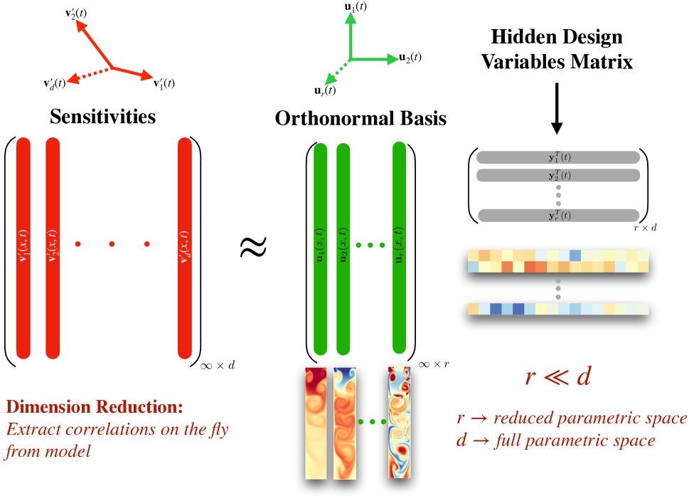
where 𝐕(x,t)=[𝐯1(x,t)|𝐯2(x,t)||𝐯d(x,t)]×dsuperscript𝐕𝑥𝑡subscriptdelimited-[]conditionalsubscriptsuperscript𝐯1𝑥𝑡subscriptsuperscript𝐯2𝑥𝑡subscriptsuperscript𝐯𝑑𝑥𝑡𝑑\mathbf{V}^{\prime}(x,t)=\big{[}\mathbf{v}^{\prime}_{1}(x,t)\ \big{|}\ \mathbf{v}^{\prime}_{2}(x,t)\ \big{|}\ \dots\ \big{|}\ \mathbf{v}^{\prime}_{d}(x,t)\big{]}_{\infty\times d} is the sensitivities quasimatrix, 𝐔(x,t)=[𝐮1(x,t)|𝐮2(x,t)||𝐮r(x,t)]×r𝐔𝑥𝑡subscriptdelimited-[]conditionalsubscript𝐮1𝑥𝑡subscript𝐮2𝑥𝑡subscript𝐮𝑟𝑥𝑡𝑟\mathbf{U}(x,t)=\big{[}\mathbf{u}_{1}(x,t)\ \big{|}\ \mathbf{u}_{2}(x,t)\ \big{|}\ \dots\ \big{|}\ \mathbf{u}_{r}(x,t)\big{]}_{\infty\times r} is a quasimatrix representing a rank-r𝑟r time-dependent orthonormal basis, in which <𝐮i(x,t),𝐮j(x,t)>=δijformulae-sequenceabsentsubscript𝐮𝑖𝑥𝑡subscript𝐮𝑗𝑥𝑡subscript𝛿𝑖𝑗\big{<}\mathbf{u}_{i}(x,t),\mathbf{u}_{j}(x,t)\big{>}=\delta_{ij}, 𝐘(t)=[𝐲1(t)|𝐲2(t)||𝐲r(t)]d×r𝐘𝑡subscriptdelimited-[]conditionalsubscript𝐲1𝑡subscript𝐲2𝑡subscript𝐲𝑟𝑡𝑑𝑟\mathbf{Y}(t)=\big{[}\mathbf{y}_{1}(t)\ \big{|}\ \mathbf{y}_{2}(t)\ \big{|}\ \dots\ \big{|}\ \mathbf{y}_{r}(t)\big{]}_{d\times r} is the coefficient matrix, and 𝐄(x,t)×d𝐄𝑥𝑡superscript𝑑\mathbf{E}(x,t)\in\mathbb{R}^{\infty\times d} is the approximation error. The f-OTD decomposition is shown schematically in Figure 1.
Refer to caption
Figure 1: Overview of the reduced order modeling strategy. Shown on left in red is the full dimensional system of sensitivities that we seek to model using the f-OTD low-rank approximation. Shown on right is the low-rank approximation which consists of a set of temporally evolving orthonormal modes (green) and hidden design variables (gray). The hidden design variables are coefficients that map the orthonormal basis to each sensitivity in the full-dimensional system. That is, each of the d𝑑d sensitivities are approximated as a linear combination of the r𝑟r orthonormal modes, where rdmuch-less-than𝑟𝑑r\ll d. It is important to note that the orthonormal basis and hidden design variables are model-driven and evolve based on the linear sensitivity dynamics. Thus, the proposed method only requires solving a system of r𝑟r PDEs and r𝑟r ODEs for the modes and coefficients, respectively.

We formulate a variational principle with control parameters 𝐔˙(x,t)˙𝐔𝑥𝑡\dot{\mathbf{U}}(x,t) and 𝐘˙(t)˙𝐘𝑡\dot{\mathbf{Y}}(t), that seeks to optimally update the subspace 𝐔(x,t)𝐔𝑥𝑡\mathbf{U}(x,t) and its coefficients 𝐘(t)𝐘𝑡\mathbf{Y}(t) by minimizing the distance between the time derivative of the low-rank approximation and the full-dimensional sensitivity dynamics:

(𝐔˙(x,t),𝐘˙(t))=(𝐔(x,t)𝐘(t)T)t(𝐔(x,t)𝐘(t)T)𝐅(x,t;𝜶)F2.˙𝐔𝑥𝑡˙𝐘𝑡superscriptsubscriptnorm𝐔𝑥𝑡𝐘superscript𝑡𝑇𝑡𝐔𝑥𝑡𝐘superscript𝑡𝑇superscript𝐅𝑥𝑡𝜶𝐹2\mathcal{F}(\dot{\mathbf{U}}(x,t),\dot{\mathbf{Y}}(t))=\left\|\dfrac{\partial(\mathbf{U}(x,t)\mathbf{Y}(t)^{T})}{\partial t}-\mathcal{L}\left(\mathbf{U}(x,t)\mathbf{Y}(t)^{T}\right)-\mathbf{F}^{\prime}(x,t;\boldsymbol{\alpha})\right\|_{F}^{2}. (5)

where 𝐅(x,t)=[𝐟1(x,t)|𝐟2(x,t)||𝐟d(x,t)]×dsuperscript𝐅𝑥𝑡subscriptdelimited-[]conditionalsubscriptsuperscript𝐟1𝑥𝑡subscriptsuperscript𝐟2𝑥𝑡subscriptsuperscript𝐟𝑑𝑥𝑡𝑑\mathbf{F}^{\prime}(x,t)=\big{[}\mathbf{f}^{\prime}_{1}(x,t)\ \big{|}\ \mathbf{f}^{\prime}_{2}(x,t)\ \big{|}\ \dots\ \big{|}\ \mathbf{f}^{\prime}_{d}(x,t)\big{]}_{\infty\times d}. Taking the time derivative of the orthonormality condition leads to the following constraint for the minimization problem:

<𝐮˙i(x,t),𝐮j(x,t)>+<𝐮i(x,t),𝐮˙j(x,t)>=0.\big{<}\dot{\mathbf{u}}_{i}(x,t),\mathbf{u}_{j}(x,t)\big{>}+\big{<}\mathbf{u}_{i}(x,t),\dot{\mathbf{u}}_{j}(x,t)\big{>}=0. (6)

We denote ϕij(t)=<𝐮i(x,t),𝐮˙j(x,t)>\boldsymbol{\phi}_{ij}(t)=\big{<}\mathbf{u}_{i}(x,t),\dot{\mathbf{u}}_{j}(x,t)\big{>}, in which 𝚽(t)=[ϕij(t)]r×r𝚽𝑡delimited-[]subscriptitalic-ϕ𝑖𝑗𝑡superscript𝑟𝑟\boldsymbol{\Phi}(t)=[\phi_{ij}(t)]\in\mathbb{R}^{r\times r}. It is easy to see that 𝚽(t)𝚽𝑡\boldsymbol{\Phi}(t) must be a skew-symmetric matrix in order to satisfy Equation 6, i.e., ϕji(t)=ϕij(t)subscriptbold-italic-ϕ𝑗𝑖𝑡subscriptbold-italic-ϕ𝑖𝑗𝑡\boldsymbol{\phi}_{ji}(t)=-\boldsymbol{\phi}_{ij}(t). Incorporating this constraint leads to the following unconstrained optimization problem functional:

𝒢(𝐔˙(x,t),𝐘˙(t),λ(t))𝒢˙𝐔𝑥𝑡˙𝐘𝑡𝜆𝑡\displaystyle\mathcal{G}(\dot{\mathbf{U}}(x,t),\dot{\mathbf{Y}}(t),\lambda(t)) =(𝐔(x,t)𝐘(t)T)t(𝐔(x,t))𝐘(t)T𝐅(x,t;𝜶)F2absentsuperscriptsubscriptnorm𝐔𝑥𝑡𝐘superscript𝑡𝑇𝑡𝐔𝑥𝑡𝐘superscript𝑡𝑇superscript𝐅𝑥𝑡𝜶𝐹2\displaystyle=\left\|\dfrac{\partial(\mathbf{U}(x,t)\mathbf{Y}(t)^{T})}{\partial t}-\mathcal{L}\left(\mathbf{U}(x,t)\right)\mathbf{Y}(t)^{T}-\mathbf{F}^{\prime}(x,t;\boldsymbol{\alpha})\right\|_{F}^{2} (7)
+i,j=1rλij(t)(<𝐮i(x,t),𝐮˙j(x,t)>ϕij(t)),\displaystyle+\sum_{i,j=1}^{r}\lambda_{ij}(t)\big{(}\big{<}\mathbf{u}_{i}(x,t),\dot{\mathbf{u}}_{j}(x,t)\big{>}-\boldsymbol{\phi}_{ij}(t)\big{)},

where λ(t)=[λij(t)]r×r𝜆𝑡delimited-[]subscript𝜆𝑖𝑗𝑡superscript𝑟𝑟\lambda(t)=[\lambda_{ij}(t)]\in\mathbb{R}^{r\times r} are Lagrange multipliers. To derive the optimality conditions, we follow a procedure similar to the one that was recently presented in [22]. In Appendix A, we show that minimizing the above functional with respect to 𝐔˙(x,t)˙𝐔𝑥𝑡\dot{\mathbf{U}}(x,t) and 𝐘˙(t)˙𝐘𝑡\dot{\mathbf{Y}}(t) leads to closed form evolution equations for the modes and corresponding sensitivity coefficients:

𝐮i(x,t)tsubscript𝐮𝑖𝑥𝑡𝑡\displaystyle\dfrac{\partial\mathbf{u}_{i}(x,t)}{\partial t} =(𝐮i)<𝐮j,(𝐮i)>𝐮j+[𝐅𝐲k<𝐮j,𝐅𝐲k>𝐮j]Cik1ϕij𝐮j,formulae-sequenceabsentlimit-fromsubscript𝐮𝑖subscript𝐮𝑗subscript𝐮𝑖subscript𝐮𝑗delimited-[]formulae-sequencelimit-fromsuperscript𝐅subscript𝐲𝑘subscript𝐮𝑗superscript𝐅subscript𝐲𝑘subscript𝐮𝑗superscriptsubscript𝐶𝑖𝑘1subscriptitalic-ϕ𝑖𝑗subscript𝐮𝑗\displaystyle=\mathcal{L}\left(\mathbf{u}_{i}\right)-\big{<}\mathbf{u}_{j},\mathcal{L}\left(\mathbf{u}_{i}\right)\big{>}\mathbf{u}_{j}+\big{[}\mathbf{F}^{\prime}\mathbf{y}_{k}-\big{<}\mathbf{u}_{j},\mathbf{F}^{\prime}\mathbf{y}_{k}\big{>}\mathbf{u}_{j}\big{]}C_{ik}^{-1}-\phi_{ij}\mathbf{u}_{j}, (8)
d𝐲i(t)dt𝑑subscript𝐲𝑖𝑡𝑑𝑡\displaystyle\frac{d\mathbf{y}_{i}(t)}{dt} =<𝐮i,(𝐮j)>𝐲j+<𝐅,𝐮i>ϕij𝐲j,\displaystyle=\big{<}\mathbf{u}_{i},\mathcal{L}(\mathbf{u}_{j})\big{>}\mathbf{y}_{j}+\big{<}\mathbf{F}^{\prime},\mathbf{u}_{i}\big{>}-\phi_{ij}\mathbf{y}_{j}, (9)

where 𝐂(t)=[Cik(t)]r×r𝐂𝑡delimited-[]subscript𝐶𝑖𝑘𝑡superscript𝑟𝑟\mathbf{C}(t)=[C_{ik}(t)]\in\mathbb{R}^{r\times r} is the low-rank correlation matrix, in which Cik(t)=𝐲i(t)T𝐲k(t)subscript𝐶𝑖𝑘𝑡subscript𝐲𝑖superscript𝑡𝑇subscript𝐲𝑘𝑡C_{ik}(t)=\mathbf{y}_{i}(t)^{T}\mathbf{y}_{k}(t). These equations are initialized by solving Equation 3 for a single time step and computing the singular value decomposition (SVD) of 𝐕(x,t=Δt)superscript𝐕𝑥𝑡Δ𝑡\mathbf{V}^{\prime}(x,t=\Delta t), such that 𝐔(x,t=Δt)𝐔𝑥𝑡Δ𝑡\mathbf{U}(x,t=\Delta t) contains the first r𝑟r left singular vectors and 𝐘(t=Δt)𝐘𝑡Δ𝑡\mathbf{Y}(t=\Delta t) is the matrix multiplication of the first r𝑟r right singular vectors and singular values; see Section 2.5. We show in Section 2.3 that the skew symmetric matrix ϕijsubscriptitalic-ϕ𝑖𝑗\phi_{ij} can be taken to be zero, i.e., ϕij=0subscriptitalic-ϕ𝑖𝑗0\phi_{ij}=0.

In the following, we make several observations about Equations 8 and 9: (i) Equation 8 determines the evolution of the f-OTD subspace. For ϕij=0subscriptitalic-ϕ𝑖𝑗0\phi_{ij}=0, the right hand side of Equation 8 is equal to the projection of (𝐔)+𝐅𝐘𝐂1𝐔superscript𝐅𝐘𝐂1\mathcal{L}\left(\mathbf{U}\right)+\mathbf{F}\mathbf{Y}\mathbf{C}^{-1} onto the complement of the space spanned by 𝐔𝐔\mathbf{U}. Therefore, if (𝐔)+𝐅𝐘𝐂1𝐔superscript𝐅𝐘𝐂1\mathcal{L}\left(\mathbf{U}\right)+\mathbf{F}\mathbf{Y}\mathbf{C}^{-1} is in the span of 𝐔𝐔\mathbf{U}, the f-OTD subspace does not evolve, i.e., 𝐔˙=𝟎˙𝐔0\dot{\mathbf{U}}=\mathbf{0}. However, when (𝐔)+𝐅𝐘𝐂1𝐔superscript𝐅𝐘𝐂1\mathcal{L}\left(\mathbf{U}\right)+\mathbf{F}\mathbf{Y}\mathbf{C}^{-1} is not in the span of 𝐔𝐔\mathbf{U}, the f-OTD subspace evolves optimally to follow the right hand side. Equation 9 is the f-OTD reduced order model (ROM) that determines the evolution of the sensitivities within the f-OTD subspace. (ii) We observe that if we set 𝐅(x,t)=𝟎superscript𝐅𝑥𝑡0\mathbf{F}^{\prime}(x,t)=\mathbf{0} in the above equations, we recover the OTD evolution equations presented in [8]. However, unlike the OTD equations, where the evolution of the OTD modes are independent of the evolution of the coefficients (𝐘𝐘\mathbf{Y}), there is a two-way nonlinear coupling between the f-OTD evolution equations for 𝐔𝐔\mathbf{U} and 𝐘𝐘\mathbf{Y}. (iii) From the above equations, it is clear to see that f-OTD extracts the low-rank approximation directly from the sensitivity evolution equation. In that sense, it is different from data-driven low-rank approximations such as proper orthogonal decomposition [23, 24, 25] or dynamic mode decomposition [26, 27], in which the low rank subspace is extracted from preexisting data. The need to generate data simply does not exist in the f-OTD workflow. (iv) The computational cost of solving the f-OTD Equations 8 and 9 is roughly equivalent to that of solving r𝑟r forward sensitivity equations. This is because the evolution of the f-OTD modes described by Equation 8 inherits the same differential operators from the sensitivity equation and the computational cost of solving each f-OTD mode is roughly equivalent to that of solving the sensitivity equation for a single parameter. Equation 9 is an ODE and therefore its computational cost is negligible compared to the f-OTD modes, which are governed by a PDE.

2.3 Equivalence

It is important to note that the choice of ϕijsubscriptitalic-ϕ𝑖𝑗\phi_{ij} in Equations 8 and 9 is not unique, and any skew-symmetric matrix yields an equivalent reduction. Similar to the OTD equations [8], we choose ϕij=0subscriptitalic-ϕ𝑖𝑗0\phi_{ij}=0, which corresponds to the dynamically orthogonal (DO) condition. This property is summarized in the theorem below.

Theorem 2.1

Let {𝐔(x,t),𝐘(t)}𝐔𝑥𝑡𝐘𝑡\{\mathbf{U}(x,t),\mathbf{Y}(t)\} and {𝐔~(x,t),𝐘~(t)}~𝐔𝑥𝑡~𝐘𝑡\{\tilde{\mathbf{U}}(x,t),\tilde{\mathbf{Y}}(t)\} represent two reductions that satisfy Equations 8 and 9 with corresponding skew-symmetric matrices 𝚽(t)𝚽𝑡\boldsymbol{\Phi}(t) and 𝚽~(t)~𝚽𝑡\tilde{\boldsymbol{\Phi}}(t), respectively. If the reductions are equivalent at t=0𝑡0t=0, i.e. they are initially related by an orthogonal rotation matrix 𝐑0r×rsubscript𝐑0superscript𝑟𝑟\mathbf{R}_{0}\in\mathbb{R}^{r\times r} as 𝐔(x,0)=𝐔~(x,0)𝐑0𝐔𝑥0~𝐔𝑥0subscript𝐑0\mathbf{U}(x,0)=\tilde{\mathbf{U}}(x,0)\mathbf{R}_{0} and 𝐘(0)=𝐘~(0)𝐑0𝐘0~𝐘0subscript𝐑0\mathbf{Y}(0)=\tilde{\mathbf{Y}}(0)\mathbf{R}_{0}, then the two reductions will remain equivalent for t>0𝑡0t>0 with rotation matrix 𝐑(t)𝐑𝑡\mathbf{R}(t) governed by 𝐑˙=𝐑𝚽𝚽~𝐑˙𝐑𝐑𝚽~𝚽𝐑\dot{\mathbf{R}}=\mathbf{R}\boldsymbol{\Phi}-\tilde{\boldsymbol{\Phi}}\mathbf{R}.

For proof of the above theorem see Appendix B.

2.4 Exactness of f-OTD

For the case where the full sensitivity quasimatrix is of rank d𝑑d, the rank d𝑑d f-OTD equations are exact. To show this, we start by considering an arbitrary perturbation subspace, 𝐕(x,t)×dsuperscript𝐕𝑥𝑡superscript𝑑\mathbf{V}^{\prime}(x,t)\in\mathbb{R}^{\infty\times d}, governed by the quasimatrix form of Equation 3:

𝐕t=(𝐕)+𝐅(x,t),𝐕(x,0)=𝐕0(x),formulae-sequencesuperscript𝐕𝑡superscript𝐕superscript𝐅𝑥𝑡superscript𝐕𝑥0subscriptsuperscript𝐕0𝑥\displaystyle\dfrac{\partial\mathbf{V}^{\prime}}{\partial t}=\mathcal{L}(\mathbf{V}^{\prime})+\mathbf{F}^{\prime}(x,t),\quad\mathbf{V}^{\prime}(x,0)=\mathbf{V}^{\prime}_{0}(x),

where columns of 𝐕(x,t)superscript𝐕𝑥𝑡\mathbf{V}^{\prime}(x,t) are independent, i.e. <𝐯i,𝐯j>=0formulae-sequenceabsentsuperscriptsubscript𝐯𝑖superscriptsubscript𝐯𝑗0\big{<}\mathbf{v}_{i}^{\prime},\mathbf{v}_{j}^{\prime}\big{>}=0 if ij𝑖𝑗i\neq j, and the evolution of an orthonormal subspace, 𝐔(x,t)×d𝐔𝑥𝑡superscript𝑑\mathbf{U}(x,t)\in\mathbb{R}^{\infty\times d}, governed by the quasimatrix form of Equation 8:

𝐔t=(𝐔)𝐔𝐋r(t)+(𝐅𝐘𝐔<𝐔,𝐅𝐘>)𝐂1,𝐔(x,0)=𝐔0(x).\displaystyle\dfrac{\partial\mathbf{U}}{\partial t}=\mathcal{L}(\mathbf{U})-\mathbf{U}\mathbf{L}_{r}(t)+\left(\mathbf{F}^{\prime}\mathbf{Y}-\mathbf{U}\big{<}\mathbf{U},\mathbf{F}^{\prime}\mathbf{Y}\big{>}\right)\mathbf{C}^{-1},\quad\mathbf{U}(x,0)=\mathbf{U}_{0}(x).

The corresponding matrix of sensitivity coefficients are governed by the matrix form of Equation 9 as:

d𝐘dt=𝐘𝐋rT+<𝐅,𝐔>,𝐘(0)=𝐘0,\displaystyle\frac{d\mathbf{Y}}{dt}=\mathbf{Y}\mathbf{L}_{r}^{T}+\big{<}\mathbf{F}^{\prime},\mathbf{U}\big{>},\quad\mathbf{Y}(0)=\mathbf{Y}_{0},

where 𝐋r(t)=<𝐔(x,t),(𝐔(x,t))>\mathbf{L}_{r}(t)=\big{<}\mathbf{U}(x,t),\mathcal{L}(\mathbf{U}(x,t))\big{>} is the r×r𝑟𝑟r\times r low-rank linear operator. We can show that if the two subspaces are initially equivalent, i.e., 𝐔0(x)subscript𝐔0𝑥\mathbf{U}_{0}(x) can be mapped to 𝐕0(x)subscriptsuperscript𝐕0𝑥\mathbf{V}^{\prime}_{0}(x) via the linear transformation 𝐘0Tsuperscriptsubscript𝐘0𝑇\mathbf{Y}_{0}^{T}, then 𝐕(x,t)superscript𝐕𝑥𝑡\mathbf{V}^{\prime}(x,t) and 𝐔(x,t)𝐔𝑥𝑡\mathbf{U}(x,t) remain equivalent for all time t𝑡t and are related by the linear transformation 𝐘(t)T𝐘superscript𝑡𝑇\mathbf{Y}(t)^{T}. This leads to the following theorem:

Theorem 2.2

Let 𝐕(x,t)×dsuperscript𝐕𝑥𝑡superscript𝑑\mathbf{V}^{\prime}(x,t)\in\mathbb{R}^{\infty\times d} be an arbitrary subspace evolved by the linear dynamics of Equation 3, and 𝐔(x,t)×d𝐔𝑥𝑡superscript𝑑\mathbf{U}(x,t)\in\mathbb{R}^{\infty\times d} be an orthonormal subspace evolved by Equation 8. If initially 𝐕0(x)subscriptsuperscript𝐕0𝑥\mathbf{V}^{\prime}_{0}(x) and 𝐔0(x)subscript𝐔0𝑥\mathbf{U}_{0}(x) are equivalent, i.e. 𝐕0(X)=𝐔0(x)𝐘0Tsubscriptsuperscript𝐕0𝑋subscript𝐔0𝑥superscriptsubscript𝐘0𝑇\mathbf{V}^{\prime}_{0}(X)=\mathbf{U}_{0}(x)\mathbf{Y}_{0}^{T}, then the perturbation subspace can be exactly determined via the linear transformation 𝐕(x,t)=𝐔(x,t)𝐘(t)Tsuperscript𝐕𝑥𝑡𝐔𝑥𝑡𝐘superscript𝑡𝑇\mathbf{V}^{\prime}(x,t)=\mathbf{U}(x,t)\mathbf{Y}(t)^{T} for all time t𝑡t, where 𝐘(t)𝐘𝑡\mathbf{Y}(t) is governed by Equation 9.

For a detailed proof of the theorem, refer to Appendix C.

2.5 Approximation error

The approximation error of estimating sensitivities using f-OTD can be expressed as e(t)=𝐕(x,t)𝐔(x,t)𝐘(t)TF𝑒𝑡subscriptnormsuperscript𝐕𝑥𝑡𝐔𝑥𝑡𝐘superscript𝑡𝑇𝐹e(t)=\|\mathbf{V}^{\prime}(x,t)-\mathbf{U}(x,t)\mathbf{Y}(t)^{T}\|_{F}. This error can be properly analyzed and better understood by considering two types of error: (i) the resolved error, denoted by er(t)subscript𝑒𝑟𝑡e_{r}(t) and (ii) the unresolved error, denoted by eu(t)subscript𝑒𝑢𝑡e_{u}(t). The resolved error is the discrepancy between approximating the sensitivities with rank-r𝑟r f-OTD and the optimal rank-r𝑟r approximation: er(t)=𝐔(x,t)𝐘(t)T𝐔~(x,t)𝐘~(t)TFsubscript𝑒𝑟𝑡subscriptnorm𝐔𝑥𝑡𝐘superscript𝑡𝑇~𝐔𝑥𝑡~𝐘superscript𝑡𝑇𝐹e_{r}(t)=\|\mathbf{U}(x,t)\mathbf{Y}(t)^{T}-\tilde{\mathbf{U}}(x,t)\tilde{\mathbf{Y}}(t)^{T}\|_{F}, where 𝐔~(x,t)×r~𝐔𝑥𝑡superscript𝑟\tilde{\mathbf{U}}(x,t)\in\mathbb{R}^{\infty\times r} and 𝐘~(t)d×r~𝐘𝑡superscript𝑑𝑟\tilde{\mathbf{Y}}(t)\in\mathbb{R}^{d\times r} are the optimal rank-r𝑟r orthonormal modes and their coefficients, respectively. The unresolved error is the error of the optimal rank-r𝑟r approximation: eu(t)=𝐔~(x,t)𝐘~(t)T𝐕(x,t)Fsubscript𝑒𝑢𝑡subscriptnorm~𝐔𝑥𝑡~𝐘superscript𝑡𝑇superscript𝐕𝑥𝑡𝐹e_{u}(t)=\|\tilde{\mathbf{U}}(x,t)\tilde{\mathbf{Y}}(t)^{T}-\mathbf{V}^{\prime}(x,t)\|_{F}, that is a direct result of truncating the dr𝑑𝑟d-r least energetic modes. Thus, the optimal rank-r𝑟r approximation is obtained by minimizing:

u(𝐔~(x,t),𝐘~(t))=𝐔~(x,t)𝐘~(t)T𝐕(x,t)F,subscript𝑢~𝐔𝑥𝑡~𝐘𝑡subscriptnorm~𝐔𝑥𝑡~𝐘superscript𝑡𝑇superscript𝐕𝑥𝑡𝐹\mathcal{E}_{u}(\tilde{\mathbf{U}}(x,t),\tilde{\mathbf{Y}}(t))=\left\|\tilde{\mathbf{U}}(x,t)\tilde{\mathbf{Y}}(t)^{T}-\mathbf{V}^{\prime}(x,t)\right\|_{F}, (10)

subject to the orthonormality condition of 𝐔~(x,t)~𝐔𝑥𝑡\tilde{\mathbf{U}}(x,t) modes. The optimal decomposition can be obtained by performing instantaneous SVD of the sensitivity matrix, where 𝐔~(x,t)~𝐔𝑥𝑡\tilde{\mathbf{U}}(x,t) is the matrix of r𝑟r most dominant left singular vectors of 𝐕(x,t)superscript𝐕𝑥𝑡\mathbf{V}^{\prime}(x,t) and 𝐘~(t)=𝐙~(t)𝚺~(t)~𝐘𝑡~𝐙𝑡~𝚺𝑡\tilde{\mathbf{Y}}(t)=\tilde{\mathbf{Z}}(t)\tilde{\mathbf{\Sigma}}(t), where 𝐙~(t)d×r~𝐙𝑡superscript𝑑𝑟\tilde{\mathbf{Z}}(t)\in\mathbb{R}^{d\times r} and 𝚺~(t)=diag(σ~1(t),σ2~(t),,σ~r(t))~𝚺𝑡diagsubscript~𝜎1𝑡~subscript𝜎2𝑡subscript~𝜎𝑟𝑡\tilde{\mathbf{\Sigma}}(t)=\mbox{diag}(\tilde{\mathbf{\sigma}}_{1}(t),\tilde{\mathbf{\sigma}_{2}}(t),\dots,\tilde{\mathbf{\sigma}}_{r}(t)) are the matrix of the r𝑟r most dominant right singular vectors and the matrix of singular values, respectively. It is straightforward to show that: eu(t)=(i=r+1dσ~i2(t))1/2subscript𝑒𝑢𝑡superscriptsuperscriptsubscript𝑖𝑟1𝑑superscriptsubscript~𝜎𝑖2𝑡12e_{u}(t)=(\sum_{i=r+1}^{d}\tilde{\sigma}_{i}^{2}(t))^{1/2}. The error eu(t)subscript𝑒𝑢𝑡e_{u}(t) represents the minimum error that any rank-r𝑟r approximation can achieve, and therefore, it amounts to a lower bound for the f-OTD error: e(t)eu(t)𝑒𝑡subscript𝑒𝑢𝑡e(t)\geq e_{u}(t). On the other hand, as with any reduced order model of a time-dependent system, the unresolved subspace induces a memory error in the f-OTD approximation. This means that the unresolved error drives the resolved error er(t)subscript𝑒𝑟𝑡e_{r}(t), and under appropriate conditions, it has been shown that for similar time-dependent basis low-rank approximations, er(t)subscript𝑒𝑟𝑡e_{r}(t) can be bounded by: er(t)c1ec2tt0teu(s)𝑑ssubscript𝑒𝑟𝑡subscript𝑐1superscript𝑒subscript𝑐2𝑡superscriptsubscriptsubscript𝑡0𝑡subscript𝑒𝑢𝑠differential-d𝑠e_{r}(t)\leq c_{1}e^{c_{2}t}\int_{t_{0}}^{t}e_{u}(s)ds [28] for c1,c2>0subscript𝑐1subscript𝑐20c_{1},c_{2}>0. The interplay between eu(t)subscript𝑒𝑢𝑡e_{u}(t) and er(t)subscript𝑒𝑟𝑡e_{r}(t) can be more rigorously studied within the Mori-Zwanzig formalism [29]. These error estimates can guide an adaptive f-OTD, in which modes are added or removed to maintain the error below some threshold value [16], however these aspects are not in the scope of this paper and are not explored any further here. Since sensitivities can either be very small or very large with errors following the same trend, we compute the relative error percentages as shown here:

% Error=e(t)𝐕(x,t)F×100.% Error𝑒𝑡subscriptnormsuperscript𝐕𝑥𝑡𝐹100\text{\% Error}=\frac{e(t)}{\left\|\mathbf{V}^{\prime}(x,t)\right\|_{F}}\times 100. (11)

Similar quantities are computed for eu(t)subscript𝑒𝑢𝑡e_{u}(t) and er(t)subscript𝑒𝑟𝑡e_{r}(t).

2.6 Mode ranking

In this section we present a procedure to rank the f-OTD modes and their coefficients according to their significance. To this end, we start by considering the reduced correlation matrix 𝐂(t)𝐂𝑡\mathbf{C}(t), which is in general a full matrix. This implies that the sensitivity coefficients are correlated and there exists a linear mapping from the correlated coefficients, 𝐘(t)𝐘𝑡\mathbf{Y}(t), to the uncorrelated coefficients, 𝐘^(t)𝚺(t)^𝐘𝑡𝚺𝑡\hat{\mathbf{Y}}(t)\boldsymbol{\Sigma}(t), where 𝐘^(t)^𝐘𝑡\hat{\mathbf{Y}}(t) are the orthonormal coefficients and 𝚺(t)=diag(σ1(t),σ2(t),,σr(t))𝚺𝑡diagsubscript𝜎1𝑡subscript𝜎2𝑡subscript𝜎𝑟𝑡\boldsymbol{\Sigma}(t)=\mbox{diag}(\sigma_{1}(t),\sigma_{2}(t),\dots,\sigma_{r}(t)) is a diagonal matrix of singular values. To find such a mapping, we consider the eigen-decomposition of 𝐂(t)𝐂𝑡\mathbf{C}(t) as follows:

𝐂(t)𝐑(t)=𝐑(t)𝚲(t),𝐂𝑡𝐑𝑡𝐑𝑡𝚲𝑡\mathbf{C}(t)\mathbf{R}(t)=\mathbf{R}(t)\boldsymbol{\Lambda}(t), (12)

where 𝐑(t)r×r𝐑𝑡superscript𝑟𝑟\mathbf{R}(t)\in\mathbb{R}^{r\times r} is a matrix whose columns contain the eigenvectors of 𝐂(t)𝐂𝑡\mathbf{C}(t) and 𝚲(t)𝚲𝑡\boldsymbol{\Lambda}(t) = diag(λ1(t),λ2(t),,λr(t)subscript𝜆1𝑡subscript𝜆2𝑡subscript𝜆𝑟𝑡\lambda_{1}(t),\lambda_{2}(t),\dots,\lambda_{r}(t)) is a diagonal matrix containing the eigenvalues of 𝐂(t)𝐂𝑡\mathbf{C}(t). Since 𝐂(t)𝐂𝑡\mathbf{C}(t) is a symmetric positive matrix, the matrix 𝐑(t)𝐑𝑡\mathbf{R}(t) is an orthonormal matrix, i.e. 𝐑(t)T𝐑(t)=𝐈𝐑superscript𝑡𝑇𝐑𝑡𝐈\mathbf{R}(t)^{T}\mathbf{R}(t)=\mathbf{I}, and the eigenvalues are all non-negative and can be sorted as: λ1(t)>λ2(t)>>λr(t)0subscript𝜆1𝑡subscript𝜆2𝑡subscript𝜆𝑟𝑡0\lambda_{1}(t)>\lambda_{2}(t)>\dots>\lambda_{r}(t)\geq 0. It is also straightforward to show that the singular values of the f-OTD low-rank approximation are σi(t)=λi(t)1/2subscript𝜎𝑖𝑡subscript𝜆𝑖superscript𝑡12\sigma_{i}(t)=\lambda_{i}(t)^{1/2}, for i=1,2,,r𝑖12𝑟i=1,2,\dots,r. The ranked f-OTD components can be defined as:

𝐘^(t)=𝐘(t)𝐑(t)𝚺1(t),𝐔^(x,t)=𝐔(x,t)𝐑(t),formulae-sequence^𝐘𝑡𝐘𝑡𝐑𝑡superscript𝚺1𝑡^𝐔𝑥𝑡𝐔𝑥𝑡𝐑𝑡\hat{\mathbf{Y}}(t)=\mathbf{Y}(t)\mathbf{R}(t)\boldsymbol{\Sigma}^{-1}(t),\quad\quad\hat{\mathbf{U}}(x,t)=\mathbf{U}(x,t)\mathbf{R}(t),

where the columns of 𝐘^(t)^𝐘𝑡\hat{\mathbf{Y}}(t) and 𝐔^(x,t)^𝐔𝑥𝑡\hat{\mathbf{U}}(x,t) are ranked by energy (σi2superscriptsubscript𝜎𝑖2\sigma_{i}^{2}) in descending order. We shall refer to {𝐘^(t),𝚺(t),𝐔^(x,t)^𝐘𝑡𝚺𝑡^𝐔𝑥𝑡\hat{\mathbf{Y}}(t),\boldsymbol{\Sigma}(t),\hat{\mathbf{U}}(x,t)} as the bi-orthonormal form of the reduction. Since the above equations are simply an in-subspace rotation, {𝐘^(t)𝚺(t),𝐔^(x,t)^𝐘𝑡𝚺𝑡^𝐔𝑥𝑡\hat{\mathbf{Y}}(t)\boldsymbol{\Sigma}(t),\hat{\mathbf{U}}(x,t)} and {𝐘(t),𝐔(x,t)𝐘𝑡𝐔𝑥𝑡\mathbf{Y}(t),\mathbf{U}(x,t)} yield equivalent low-rank approximations of the full-dimensional dynamics. This is easily verified by considering the bi-orthonormal form of the low-rank approximation as 𝐔^(x,t)𝚺(t)𝐘^(t)T^𝐔𝑥𝑡𝚺𝑡^𝐘superscript𝑡𝑇\hat{\mathbf{U}}(x,t)\boldsymbol{\Sigma}(t)\hat{\mathbf{Y}}(t)^{T} =𝐔(x,t)𝐘(t)Tabsent𝐔𝑥𝑡𝐘superscript𝑡𝑇=\mathbf{U}(x,t)\mathbf{Y}(t)^{T}, where we have made use of the identity 𝐑(t)T𝐑(t)=𝐈𝐑superscript𝑡𝑇𝐑𝑡𝐈\mathbf{R}(t)^{T}\mathbf{R}(t)=\mathbf{I}. We refer to 𝐘^^𝐘\hat{\mathbf{Y}} as the hidden parametric space as each column of matrix 𝐘^^𝐘\hat{\mathbf{Y}} can be taken as a new ranked parameter that represents the contribution of all parameters (𝜶𝜶\boldsymbol{\alpha}). In the following sections, all figures will be presented in bi-orthonormal form.

3 Demonstration Cases

3.1 Rössler system

We first present a simple demonstration of f-OTD by computing sensitivities of the Rössler system. The Rössler system is governed by:

dv1dt=v2v3,dv2dt=v1+α1v2,dv3dt=α2+v3(v1α3).formulae-sequence𝑑subscript𝑣1𝑑𝑡subscript𝑣2subscript𝑣3formulae-sequence𝑑subscript𝑣2𝑑𝑡subscript𝑣1subscript𝛼1subscript𝑣2𝑑subscript𝑣3𝑑𝑡subscript𝛼2subscript𝑣3subscript𝑣1subscript𝛼3\frac{dv_{1}}{dt}=-v_{2}-v_{3},\quad\quad\frac{dv_{2}}{dt}=v_{1}+\alpha_{1}v_{2},\quad\quad\frac{dv_{3}}{dt}=\alpha_{2}+v_{3}(v_{1}-\alpha_{3}).

In the above equations, we set α1=α2=0.1subscript𝛼1subscript𝛼20.1\alpha_{1}=\alpha_{2}=0.1 and α3=14subscript𝛼314\alpha_{3}=14, which are common values used to study the chaotic behavior of the attractor. The goal is to calculate the sensitivity of 𝐯𝐯\mathbf{v} with respect to the model parameters 𝜶=(α1,α2,α3)𝜶subscript𝛼1subscript𝛼2subscript𝛼3\boldsymbol{\alpha}=(\alpha_{1},\alpha_{2},\alpha_{3}) as 𝐯/𝜶𝐯𝜶\partial\mathbf{v}/\partial\boldsymbol{\alpha}. To this end, we take the derivative of the above system of equations with respect to model parameter αisubscript𝛼𝑖\alpha_{i} to obtain the sensitivity equation

d𝐕dt=𝐋𝐕+𝐅,𝑑superscript𝐕𝑑𝑡superscript𝐋𝐕superscript𝐅\frac{d\mathbf{V}^{\prime}}{dt}=\mathbf{L}\mathbf{V}^{\prime}+\mathbf{F}^{\prime}, (13)

where

𝐋=[0111α10v30v1α3],𝐕=[𝐯1𝐯2𝐯3],𝐅=[000v20001v3],formulae-sequence𝐋matrix0111subscript𝛼10subscript𝑣30subscript𝑣1subscript𝛼3formulae-sequencesuperscript𝐕matrixmissing-subexpressionmissing-subexpressionmissing-subexpressionsubscriptsuperscript𝐯1subscriptsuperscript𝐯2subscriptsuperscript𝐯3superscript𝐅matrix000subscript𝑣20001subscript𝑣3\mathbf{L}=\begin{bmatrix}0&-1&-1\\ 1&\alpha_{1}&0\\ v_{3}&0&v_{1}-\alpha_{3}\end{bmatrix},\quad\mathbf{V}^{\prime}=\begin{bmatrix}\vline&\vline&\vline\\ \mathbf{v}^{\prime}_{1}&\mathbf{v}^{\prime}_{2}&\mathbf{v}^{\prime}_{3}\\ \vline&\vline&\vline\end{bmatrix},\quad\mathbf{F}^{\prime}=\begin{bmatrix}0&0&0\\ v_{2}&0&0\\ 0&1&-v_{3}\end{bmatrix},

and 𝐯isubscriptsuperscript𝐯𝑖\mathbf{v}^{\prime}_{i} is the sensitivity of the position with respect to αisubscript𝛼𝑖\alpha_{i} and 𝐋n×n𝐋superscript𝑛𝑛\mathbf{L}\in\mathbb{R}^{n\times n} and 𝐅n×dsuperscript𝐅superscript𝑛𝑑\mathbf{F}^{\prime}\in\mathbb{R}^{n\times d}.

Refer to caption
Refer to caption
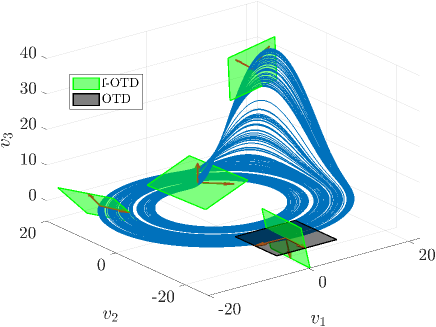
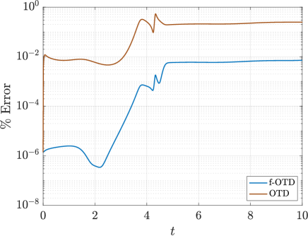
Figure 2: (a) Chaotic Rössler attractor with optimal f-OTD subspace shown in green and OTD subspace shown in black for r=2𝑟2r=2. Red arrows depict the orthonormal sensitivity vectors that define each subspace. (b) Percent error for e(t)𝑒𝑡e(t) plotted versus time for the f-OTD and OTD subspaces.

We choose a subspace with dimension r=2𝑟2r=2 for the low-rank approximation of the three-dimensional (d=3𝑑3d=3) sensitivities (𝐕superscript𝐕\mathbf{V}^{\prime}). Although it is obvious that OTD modes are not based on parametric sensitivities and they are based on perturbations in the initial condition (IC) in all directions of the phase space, we believe it is instructive to contrast the OTD versus f-OTD to better understand f-OTD. To this end, we build two real-time ROMs using OTD modes and f-OTD modes. In the case of OTD, we solve the OTD evolution equation and we project the forced sensitivity Equation 13 onto the OTD modes, resulting in:

d𝐔otddt=(𝐈𝐔otd𝐔otdT)𝐋𝐔otdandd𝐘otddt=𝐘otd𝐔otdT𝐋T𝐔otd+𝐅T𝐔otd.𝑑subscript𝐔𝑜𝑡𝑑𝑑𝑡𝐈subscript𝐔𝑜𝑡𝑑superscriptsubscript𝐔𝑜𝑡𝑑𝑇subscript𝐋𝐔𝑜𝑡𝑑and𝑑subscript𝐘𝑜𝑡𝑑𝑑𝑡subscript𝐘𝑜𝑡𝑑subscriptsuperscript𝐔𝑇𝑜𝑡𝑑superscript𝐋𝑇subscript𝐔𝑜𝑡𝑑superscript𝐅𝑇subscript𝐔𝑜𝑡𝑑\frac{d\mathbf{U}_{otd}}{dt}=(\mathbf{I}-\mathbf{U}_{otd}\mathbf{U}_{otd}^{T})\mathbf{L}\mathbf{U}_{otd}\quad\mbox{and}\quad\frac{d\mathbf{Y}_{otd}}{dt}=\mathbf{Y}_{otd}\mathbf{U}^{T}_{otd}\mathbf{L}^{T}\mathbf{U}_{otd}+\mathbf{F}^{\prime T}\mathbf{U}_{otd}.

We also solved the f-OTD evolution Equations 8 and 9 for the finite-dimensional system. Both OTD and f-OTD modes are initialized with the same subspace and the evolution equations are solved for Tf=10subscript𝑇𝑓10T_{f}=10 units of time. These subspaces are initialized by first solving the full-dimensional sensitivity Equation 13 for one Δt=102Δ𝑡superscript102\Delta t=10^{-2} and then computing the OTD and f-OTD subspaces as the first two left singular vectors of 𝐕(x,t=Δt)superscript𝐕𝑥𝑡Δ𝑡\mathbf{V}^{\prime}(x,t=\Delta t). In Figure 2, both OTD and f-OTD subspaces are visualized along with the attractor of the Rössler system. The OTD subspace is shown at only one instant for clarity and that point corresponds to the case where the nonlinear dynamics is in the v1v2subscript𝑣1subscript𝑣2v_{1}-v_{2} plane. At this point, the OTD subspace is oriented such that it nearly coincides with the v1v2subscript𝑣1subscript𝑣2v_{1}-v_{2} plane. This result is to be expected since the OTD subspace follows the sensitivities associated with the perturbations in the IC and we know that the IC-perturbed solutions will lie on the same attractor. On the other hand, the f-OTD subspace is correctly oriented along the most sensitive subspace for perturbations in the model parameters, i.e. δ𝜶=(δα1,δα2,δα3)𝛿𝜶𝛿subscript𝛼1𝛿subscript𝛼2𝛿subscript𝛼3\delta\boldsymbol{\alpha}=(\delta\alpha_{1},\delta\alpha_{2},\delta\alpha_{3}), which lead to perturbations in the attractor itself. That is, the perturbed solutions lie on different attractors which can readily be seen as δ𝜶𝛿𝜶\delta\boldsymbol{\alpha} results in nonzero δv3𝛿subscript𝑣3\delta v_{3}, despite v30similar-to-or-equalssubscript𝑣30v_{3}\simeq 0. This results in the f-OTD subspace having a large out-of-plane component in the v3subscript𝑣3v_{3} direction, which the OTD subspace fails to capture in Figure 2. In Figure 2, the percent errors of e(t)𝑒𝑡e(t) are shown for OTD and f-OTD, which confirms that f-OTD performs significantly better than OTD. This simple example demonstrates that the OTD basis is not optimal and may be inaccurate for reduced order modeling of the forced sensitivity equation.

3.2 Chaotic Kuramoto Sivashinsky equation

The objective of this example is to evaluate the performance of f-OTD in computing sensitivities of a chaotic system with many positive Lyapunov exponents and a high-dimensional parametric space. The intent of this example is not to compute the gradient of a time-averaged quantity for a chaotic system, but rather computing the solution of the sensitivity equation for a chaotic system with much larger unstable directions than the rank of the f-OTD subspace. For computing sensitivities of time-averaged quantities, one can use f-OTD in conjunction with Ruelle’s linear response formula [30, 31] to compute ensemble sensitivities. To this end, we consider the sensitivity of the Kuramoto Sivashinsky (KS) equation with respect to a time dependent forcing parameter α(t)𝛼𝑡\alpha(t). The KS equation is a fourth order PDE given by:

𝐯t+12𝐯2x+2𝐯x2+ν4𝐯x=α(t)sin(2πx/L),x[0,L],formulae-sequence𝐯𝑡12superscript𝐯2𝑥superscript2𝐯superscript𝑥2𝜈superscript4𝐯𝑥𝛼𝑡2𝜋𝑥𝐿𝑥0𝐿\displaystyle\dfrac{\partial\mathbf{v}}{\partial t}+\frac{1}{2}\dfrac{\partial\mathbf{v}^{2}}{\partial x}+\dfrac{\partial^{2}\mathbf{v}}{\partial x^{2}}+\nu\dfrac{\partial^{4}\mathbf{v}}{\partial x}=\alpha(t)\sin{\left(2\pi x/L\right)},\quad x\in[0,L], (14)

where 𝐯=𝐯(x,t)𝐯𝐯𝑥𝑡\mathbf{v}=\mathbf{v}(x,t). Approximately 110 positive Lyapunov exponents exist for the parameters used in this study: ν=1𝜈1\nu=1 and L=1000𝐿1000L=1000. The space time solution of Equation 14 for these parameters is shown in Figure 3.

Refer to caption
Figure 3: Solution of the chaotic Kuramoto-Sivashinksy equation 𝐯(x,t)𝐯𝑥𝑡\mathbf{v}(x,t) solved on domain length L=1000𝐿1000L=1000 for Tf=100subscript𝑇𝑓100T_{f}=100 units of time.

Here α(t)𝛼𝑡\alpha(t) represents an infinite-dimensional parametric space.

To compute the sensitivities numerically, we consider a discrete representation of α(t)𝛼𝑡\alpha(t) in the interval ti[0,Ts]subscript𝑡𝑖0subscript𝑇𝑠t_{i}\in[0,T_{s}], where TsTfsubscript𝑇𝑠subscript𝑇𝑓T_{s}\leq T_{f} is a subset of the full integration time Tfsubscript𝑇𝑓T_{f}, and tisubscript𝑡𝑖t_{i} is a discrete instance in time. To this end, we consider the value of α(t)𝛼𝑡\alpha(t) at discrete time ti=(i1)×Δtsubscript𝑡𝑖𝑖1Δ𝑡t_{i}=(i-1)\times\Delta t, where ΔtΔ𝑡\Delta t is the time step. This results in a vector, 𝜶=(α1,α2,,αd)𝜶subscript𝛼1subscript𝛼2subscript𝛼𝑑\boldsymbol{\alpha}=(\alpha_{1},\alpha_{2},\dots,\alpha_{d}), where αi=α(ti)subscript𝛼𝑖𝛼subscript𝑡𝑖\alpha_{i}=\alpha(t_{i}) and d=Ts/Δt𝑑subscript𝑇𝑠Δ𝑡d=T_{s}/\Delta t is the number of instances in time (i.e. number of parameters). In general, ΔtΔ𝑡\Delta t can be chosen independently of the numerical time integration step size, however, for simplicity, we use the same value of ΔtΔ𝑡\Delta t for both the parametric discretization and numerical integration of the nonlinear solver and f-OTD equations. In this example, we consider Δt=102Δ𝑡superscript102\Delta t=10^{-2} and Ts=10subscript𝑇𝑠10T_{s}=10, which results in d=1000𝑑1000d=1000 parameters. Further decrease in ΔtΔ𝑡\Delta t did not change our results. This leads to the sensitivity of 𝐯𝐯\mathbf{v} with respect to the value of α(t)𝛼𝑡\alpha(t) at 1000 evenly spaced instances in time. We evolve these sensitivities over the interval t[0,Tf]𝑡0subscript𝑇𝑓t\in[0,T_{f}] with Tf=100subscript𝑇𝑓100T_{f}=100. We also choose α(t)=0𝛼𝑡0\alpha(t)=0 for ti[0,Tf]subscript𝑡𝑖0subscript𝑇𝑓t_{i}\in[0,T_{f}], and therefore, the nonlinear solver 𝐯(t)𝐯𝑡\mathbf{v}(t) is the solution of the unforced KS equation.

We consider the time-discrete form of Equation 14 and differentiate with respect to design parameter αisubscript𝛼𝑖\alpha_{i}. This leads to an evolution equation for the sensitivity of 𝐯𝐯\mathbf{v} with respect to αisubscript𝛼𝑖\alpha_{i}, in which the linear operator and forcing terms are:

(𝐯i)=[(𝐯𝐯i)x+2𝐯ix2+ν4𝐯ix]and𝐟i=δ(tti)sin(2πx/L),i=1,2,,dformulae-sequencesuperscriptsubscript𝐯𝑖delimited-[]superscriptsubscript𝐯𝐯𝑖𝑥superscript2subscriptsuperscript𝐯𝑖superscript𝑥2𝜈superscript4subscriptsuperscript𝐯𝑖𝑥andsuperscriptsubscript𝐟𝑖𝛿𝑡subscript𝑡𝑖2𝜋𝑥𝐿𝑖12𝑑\mathcal{L}(\mathbf{v}_{i}^{\prime})=-\left[\dfrac{\partial(\mathbf{vv}_{i}^{\prime})}{\partial x}+\dfrac{\partial^{2}\mathbf{v}^{\prime}_{i}}{\partial x^{2}}+\nu\dfrac{\partial^{4}\mathbf{v}^{\prime}_{i}}{\partial x}\right]\ \mbox{and}\ \mathbf{f}_{i}^{\prime}=\delta(t-t_{i})\sin\left(2\pi x/L\right),\ i=1,2,\dots,d (15)

where δ(tti)=0𝛿𝑡subscript𝑡𝑖0\delta(t-t_{i})=0 for tti𝑡subscript𝑡𝑖t\neq t_{i} and δ(tti)=1𝛿𝑡subscript𝑡𝑖1\delta(t-t_{i})=1 for t=ti𝑡subscript𝑡𝑖t=t_{i}. Our goal is to solve Equation 15 using f-OTD.
Refer to caption
Refer to caption
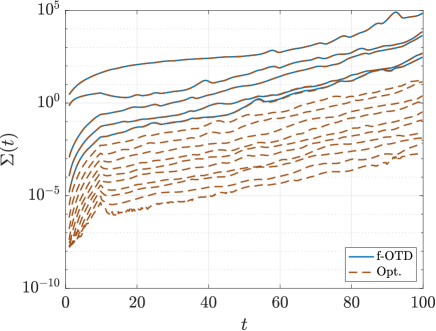
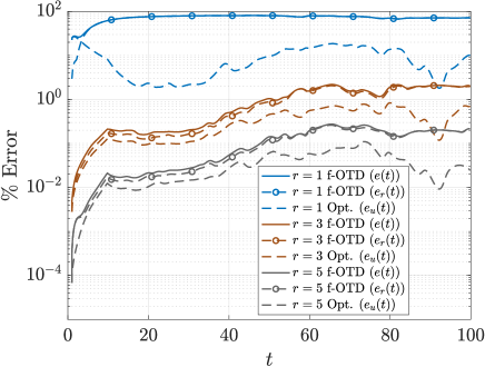
Figure 4: (a) Comparison of the reconstruction error between f-OTD approximation (e(t)𝑒𝑡e(t)) and optimal rank-r𝑟r approximation (eu(t)subscript𝑒𝑢𝑡e_{u}(t)) for different reduction sizes. Resolved error, er(t)subscript𝑒𝑟𝑡e_{r}(t), dominates the f-OTD error for long term integration. Error decreases as the number of modes increases. (b) Comparison of singular values between f-OTD and optimal low-rank decomposition for r=5𝑟5r=5.

We discretize the KS equation and the f-OTD equations using n=213=8192𝑛superscript2138192n=2^{13}=8192 Fourier modes and use exponential time-differencing Runge-Kutta fourth-order (ETDRK4) time stepping scheme [32]. We verify our solution by directly solving Equation 15 for all 1000 sensitivities. Further decreasing ΔtΔ𝑡\Delta t and increasing the number of Fourier modes did not change our results. We also compare the f-OTD error with that of optimal instantaneous same-rank approximation of the full sensitivities, which is obtained by computing the SVD of 𝐕(x,t)superscript𝐕𝑥𝑡\mathbf{V}^{\prime}(x,t) at each time. In Figure 4, we compare the reconstruction error of f-OTD (e(t)𝑒𝑡e(t)) with the reconstruction error of same-rank SVD (eu(t)subscript𝑒𝑢𝑡e_{u}(t)). We also show the resolved error er(t)subscript𝑒𝑟𝑡e_{r}(t), which measures the discrepancy between the f-OTD approximation and the optimal same-rank approximation. We compute these errors for r=1,3𝑟13r=1,3 and 5. While the optimal low-rank approximation with a single mode captures approximately 99% of the system energy of the full sensitivity (see Figure 4), the f-OTD approximation performs poorly with only a single mode, i.e., a dramatic reduction for 1000 sensitivities. This is a direct result of the memory effect from the lost interactions with the unresolved modes (er(t)subscript𝑒𝑟𝑡e_{r}(t)) that ultimately dominate the error for long term integration. By increasing the number of f-OTD modes, both e(t)𝑒𝑡e(t) and er(t)subscript𝑒𝑟𝑡e_{r}(t) decrease. It is possible to control the error in real-time through an adaptive strategy that adds/removes modes with an appropriate criterion. For example, a candidate criterion could be p=σr2(t)/i=1rσi2(t)𝑝subscriptsuperscript𝜎2𝑟𝑡superscriptsubscript𝑖1𝑟subscriptsuperscript𝜎2𝑖𝑡p=\sigma^{2}_{r}(t)/\sum_{i=1}^{r}\sigma^{2}_{i}(t), where for p<pth𝑝subscript𝑝𝑡p<p_{th} the last mode can be removed and for p>pth𝑝subscript𝑝𝑡p>p_{th} a new mode can be added. See [16] for similar strategies for adaptive mode addition and removal. In Figure 4, we compare the 15 largest instantaneous singular values of quasimatrix 𝐕(x,t)superscript𝐕𝑥𝑡\mathbf{V}^{\prime}(x,t) with those obtained from f-OTD with rank r=5𝑟5r=5, which shows that f-OTD closely captures the most dominant subspace.

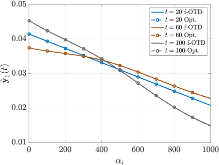
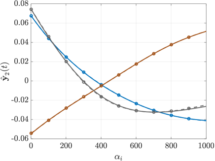
In Figures 5 and 5 the orthonormalized coefficients of the first two dominant f-OTD modes for the case of r=5𝑟5r=5 are compared to the right singular vectors from the instantaneous SVD of 𝐕(x,t)superscript𝐕𝑥𝑡\mathbf{V}^{\prime}(x,t). These coefficients represent the hidden parametric space: for example, 𝐲^1subscript^𝐲1\hat{\mathbf{y}}_{1} is a series of weights that represent the contribution of each of the d=1000𝑑1000d=1000 sensitivities to the most dominant direction of the full sensitivity matrix, 𝐮^1subscript^𝐮1\hat{\mathbf{u}}_{1}. Due to the chaotic nature of this problem, we observe that these coefficients can be highly time-dependent, especially for the lower energy modes; see 𝐲^2subscript^𝐲2\hat{\mathbf{y}}_{2}. Nevertheless, we have demonstrated that f-OTD extracts the most dominant subspace and associated coefficients of the sensitivity matrix for a chaotic system with large number of unstable directions and parameters.
Refer to caption
Refer to caption
Figure 5: Kuramoto-Sivashinsky: The first two columns of the orthonormalized design variables matrix shown at different instances in time: (a) 𝐲^1(t)subscript^𝐲1𝑡\hat{\mathbf{y}}_{1}(t) (b) 𝐲^2(t)subscript^𝐲2𝑡\hat{\mathbf{y}}_{2}(t). The horizontal axis corresponds to the ithsuperscript𝑖𝑡i^{th} design parameter αisubscript𝛼𝑖\alpha_{i}.

3.3 Species transport equation: Turbulent reactive flow

In this example, we show how a single set of f-OTD modes can lead to significant computational gains for computing sensitivities in problems with multiple coupled field variables, where each field variable has a different linear operator. We consider a species transport problem, where parameter identification via sensitivity analysis plays an important role in allocating computational and experimental resources to reduce parameter uncertainty. Moreover, the sensitivity analysis is used to create reduced reaction mechanisms for complex chemical systems involving a large number of species and reactions. See references [18, 19, 20].

Refer to caption
Figure 6: Schematic of the flow visualized with a passive scalar.

3.3.1 Problem setup

To this end, we consider a 2D incompressible turbulent reactive flow:

𝐯it+(𝐰)𝐯i=κ~ik2𝐯k+𝐬i,subscript𝐯𝑖𝑡𝐰subscript𝐯𝑖subscript~𝜅𝑖𝑘superscript2subscript𝐯𝑘subscript𝐬𝑖\dfrac{\partial\mathbf{v}_{i}}{\partial t}+\left(\mathbf{w}\cdot\nabla\right)\mathbf{v}_{i}=\tilde{\kappa}_{ik}\nabla^{2}\mathbf{v}_{k}+\mathbf{s}_{i}, (16)

where 𝐰=(𝐰x1(x1,x2,t),𝐰x2(x1,x2,t))𝐰subscript𝐰subscript𝑥1subscript𝑥1subscript𝑥2𝑡subscript𝐰subscript𝑥2subscript𝑥1subscript𝑥2𝑡\mathbf{w}=(\mathbf{w}_{x_{1}}(x_{1},x_{2},t),\mathbf{w}_{x_{2}}(x_{1},x_{2},t)) is the velocity field from the 2D incompressible Navier-Stokes equations, 𝐯i=𝐯i(x1,x2,t)subscript𝐯𝑖subscript𝐯𝑖subscript𝑥1subscript𝑥2𝑡\mathbf{v}_{i}=\mathbf{v}_{i}(x_{1},x_{2},t) is the concentration of species i𝑖i, κ~ikns×nssubscript~𝜅𝑖𝑘superscriptsubscript𝑛𝑠subscript𝑛𝑠\tilde{\kappa}_{ik}\in\mathbb{R}^{n_{s}\times n_{s}} is the diffusion coefficient matrix, and 𝐬i=𝐬i(𝐯1,𝐯2,,𝐯ns;𝜶)subscript𝐬𝑖subscript𝐬𝑖subscript𝐯1subscript𝐯2subscript𝐯subscript𝑛𝑠𝜶\mathbf{s}_{i}=\mathbf{s}_{i}(\mathbf{v}_{1},\mathbf{v}_{2},\dots,\mathbf{v}_{n_{s}};\boldsymbol{\alpha}) is the non-linear reactive source term. We choose a diagonal diffusion coefficient matrix, where the i𝑖ith diagonal entry is the diffusion coefficient of the i𝑖ith species, and nssubscript𝑛𝑠n_{s} is the number of species. For the reactive source term 𝐬isubscript𝐬𝑖\mathbf{s}_{i}, we consider the biological reactions used in [33]. These terms are listed in Table 1 in Appendix E for reference. A schematic of the flow is shown in Figure 6, where L𝐿L and H𝐻H are the channel length and height, respectively. The no-slip boundary condition is enforced at the top and bottom walls while the outflow boundary condition is enforced downstream. At the inlet a parabolic velocity with the average inlet velocity of w¯¯𝑤\overline{w} is prescribed. The Reynolds number based on reference length of half the height (H/2𝐻2H/2) and the kinematic viscosity ν𝜈\nu is Re=w¯H/2ν=1000𝑅𝑒¯𝑤𝐻2𝜈1000Re=\overline{w}H/2\nu=1000. The inlet boundary condition is 𝐯i(0,x2,t)=1/2(tanh(x2+H/2)/δtanh(x2H/2)/δ)subscript𝐯𝑖0subscript𝑥2𝑡12subscript𝑥2𝐻2𝛿subscript𝑥2𝐻2𝛿\mathbf{v}_{i}(0,x_{2},t)=1/2\big{(}\tanh{(x_{2}+H/2)/\delta}-\tanh{(x_{2}-H/2)/\delta}\big{)} for all species, where δ=0.1𝛿0.1\delta=0.1.

The velocity field is governed by two-dimensional incompressible Navier-Stokes equation. We solved the velocity field once as it is independent from the species using spectral/hp elements method with 4008 quadrilateral elements and polynomial order 5. For more details on the spectral element method see for example [34, 35, 36] . We then solve the species transport equations and f-OTD equations in the rectangular domain shown by dashed lines in Figure 6. In the rectangular domain, we used structured spectral elements with 50 elements in x1subscript𝑥1x_{1} direction and 15 elements in x2subscript𝑥2x_{2} direction. We used spectral polynomial of order 5 in each direction. The velocity field was interpolated onto this grid. The f-OTD equations, which are presented in the next sections, and the species transport equation are integrated forward in time using RK4 with Δt=5×10⁴Δ𝑡5superscript104\Delta t=5\times 10^{-4}.

3.3.2 f-OTD formulation

Our goal is to calculate sensitivity of the species concentration with respect to the reaction parameters 𝜶=(α1,α2,,αnr)𝜶subscript𝛼1subscript𝛼2subscript𝛼subscript𝑛𝑟\boldsymbol{\alpha}=(\alpha_{1},\alpha_{2},\dots,\alpha_{n_{r}}), where nrsubscript𝑛𝑟n_{r} is the number of reaction parameters. To this end, we take the derivative of the above equation with respect to reaction parameter αjsubscript𝛼𝑗\alpha_{j} to obtain an evolution equation for the sensitivity:

𝐯~ijt+(𝐰)𝐯~ij=κ~ik2𝐯~kj+~𝐬ik𝐯~kj+𝐬~ij,superscriptsubscript~𝐯𝑖𝑗𝑡𝐰superscriptsubscript~𝐯𝑖𝑗subscript~𝜅𝑖𝑘superscript2superscriptsubscript~𝐯𝑘𝑗subscript~subscript𝐬𝑖𝑘superscriptsubscript~𝐯𝑘𝑗subscriptsuperscript~𝐬𝑖𝑗\dfrac{\partial\tilde{\mathbf{v}}_{ij}^{\prime}}{\partial t}+\left(\mathbf{w}\cdot\nabla\right)\tilde{\mathbf{v}}_{ij}^{\prime}=\tilde{\kappa}_{ik}\nabla^{2}\tilde{\mathbf{v}}_{kj}^{\prime}+\tilde{\mathcal{L}}_{\mathbf{s}_{ik}}\tilde{\mathbf{v}}_{kj}^{\prime}+\tilde{\mathbf{s}}^{\prime}_{ij}, (17)

where 𝐯~ij=𝐯i/αj×1subscriptsuperscript~𝐯𝑖𝑗subscript𝐯𝑖subscript𝛼𝑗superscript1\tilde{\mathbf{v}}^{\prime}_{ij}=\partial\mathbf{v}_{i}/\partial\alpha_{j}\in\mathbb{R}^{\infty\times 1} is the sensitivity of the concentration of species 𝐯isubscript𝐯𝑖\mathbf{v}_{i} with respect to reaction rate αjsubscript𝛼𝑗\alpha_{j}, ~𝐬ik=𝐬i/𝐯ksubscript~subscript𝐬𝑖𝑘subscript𝐬𝑖subscript𝐯𝑘\tilde{\mathcal{L}}_{\mathbf{s}_{ik}}=\partial\mathbf{s}_{i}/\partial\mathbf{v}_{k} is the linearized reactive source term, and 𝐬~ij=𝐬i/αjsubscriptsuperscript~𝐬𝑖𝑗subscript𝐬𝑖subscript𝛼𝑗\tilde{\mathbf{s}}^{\prime}_{ij}=\partial\mathbf{s}_{i}/\partial\alpha_{j}. In the above equation, ~𝐬ik𝐯~kjsubscript~subscript𝐬𝑖𝑘superscriptsubscript~𝐯𝑘𝑗\tilde{\mathcal{L}}_{\mathbf{s}_{ik}}\tilde{\mathbf{v}}_{kj}^{\prime} should be interpreted as a matrix-matrix multiplication for any (x1,x2)subscript𝑥1subscript𝑥2(x_{1},x_{2}) point in the physical space. In this notation, sensitivities are represented by a quasitensor i.e. 𝐕~=[𝐯ij]superscript~𝐕delimited-[]subscriptsuperscript𝐯𝑖𝑗\tilde{\mathbf{V}}^{\prime}=[\mathbf{v}^{\prime}_{ij}] with i=1,2,,ns𝑖12subscript𝑛𝑠i=1,2,\dots,n_{s} and j=1,2,,nr𝑗12subscript𝑛𝑟j=1,2,\dots,n_{r}, where 𝐕~×ns×nrsuperscript~𝐕superscriptsubscript𝑛𝑠subscript𝑛𝑟\tilde{\mathbf{V}}^{\prime}\in\mathbb{R}^{\infty\times n_{s}\times n_{r}} is the third order quasitensor depicted in the left-hand side of Figure 7. Here ~~\tilde{\cdot} denotes terms associated with the tensor equation. In the discrete representation of 𝐕~superscript~𝐕\tilde{\mathbf{V}}^{\prime}, the dimension \infty is replaced with the number of grid points.

Solving for the sensitivities 𝐯~ijsuperscriptsubscript~𝐯𝑖𝑗\tilde{\mathbf{v}}_{ij}^{\prime} using adjoint would require solving nssubscript𝑛𝑠n_{s} AEs: one adjoint field for each species. See for example [18, 19, 20].

Refer to caption
Figure 7: Schematic of the tensor flattening from a 3D quasitensor to a 2D quasimatrix.

To solve for sensitivities using f-OTD, one could also solve for nssubscript𝑛𝑠n_{s} sets of f-OTD modes, i.e. one set of f-OTD modes for each species. This straightforward approach would only exploit the correlation between sensitivities of each species separately, i.e. correlations between 𝐯ijsubscriptsuperscript𝐯𝑖𝑗\mathbf{v}^{\prime}_{ij} for a fixed i𝑖i, while leaving the correlations between sensitivities of different species unexploited. In this example, we demonstrate how a single set of f-OTD modes can be used to accurately model the entire sensitivity tensor. Therefore, the compression ratio both in terms of memory and computational cost in comparison to the full sensitivity equation is r/d𝑟𝑑r/d. In comparison to AE, the compression ratio is r/ns𝑟subscript𝑛𝑠r/n_{s}. Also, the f-OTD is a forward system and does not impose any I/O operation. To this end, we flatten the sensitivity tensor, as shown in Figure 7, which results in a quasimatrix of size ×d𝑑\infty\times d. Here, d=ns×nr𝑑subscript𝑛𝑠subscript𝑛𝑟d=n_{s}\times n_{r}, where ns=23subscript𝑛𝑠23n_{s}=23 and nr=34subscript𝑛𝑟34n_{r}=34. This leads to a total of d=782𝑑782d=782 sensitivity equations that we seek to compute. In Appendix D, we show that the flattened sensitivity evolution equation is:

𝐯mt+(𝐰)𝐯m=κmn2𝐯n+𝐬mn𝐯n+𝐬m,subscriptsuperscript𝐯𝑚𝑡𝐰subscriptsuperscript𝐯𝑚subscript𝜅𝑚𝑛superscript2subscriptsuperscript𝐯𝑛subscriptsubscript𝐬𝑚𝑛subscriptsuperscript𝐯𝑛subscriptsuperscript𝐬𝑚\dfrac{\partial\mathbf{v}^{\prime}_{m}}{\partial t}+(\mathbf{w}\cdot\nabla)\mathbf{v}^{\prime}_{m}=\kappa_{mn}\nabla^{2}\mathbf{v}^{\prime}_{n}+\mathcal{L}_{\mathbf{s}_{mn}}\mathbf{v}^{\prime}_{n}+\mathbf{s}^{\prime}_{m}, (18)

where m(i,j)=j+(i1)nr𝑚𝑖𝑗𝑗𝑖1subscript𝑛𝑟m(i,j)=j+(i-1)n_{r} and n(i,j)=j+(i1)nr𝑛superscript𝑖superscript𝑗superscript𝑗superscript𝑖1subscript𝑛𝑟n(i^{\prime},j^{\prime})=j^{\prime}+(i^{\prime}-1)n_{r}, resulting in m,n=1,2,,dformulae-sequence𝑚𝑛12𝑑m,n=1,2,\dots,d. Equation 17 is a tensor evolution equation, whereas Equation 18 is the equivalent matrix evolution equation. The tensor flattening carried out here is similar to the unfolding carried out in the Tucker tensor decomposition [37]. However, unlike Tucker tensor decomposition we do not consider flattening the tensor in the other two dimensions of species and parameters. Each 𝐲k(t)subscript𝐲𝑘𝑡\mathbf{y}_{k}(t) is a vector of size (nsnr)×1subscript𝑛𝑠subscript𝑛𝑟1(n_{s}n_{r})\times 1 and contains coefficients for species and parameters. Once the sensitivity tensor is flattened to a quasimatrix, we use f-OTD to extract low-rank structure from the quasimatrix. In Equation 18, the linear operator changes from one species to the other due to the different diffusion coefficients κmnsubscript𝜅𝑚𝑛\kappa_{mn}. In Appendix D we show how f-OTD evolution equations can be derived for this case, which is different from the previous demonstration cases.
Refer to caption
Refer to caption
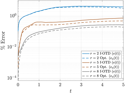
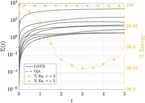
Figure 8: (a) Percent error plotted as a function of time. Error decreases as the number of modes r𝑟r increases. (b) Singular values plotted as a function of time for r=8𝑟8r=8.

We solve Equations D and D for different f-OTD ranks along with the species transport (Equation 16). In Figure 8 the f-OTD error (e(t))𝑒𝑡(e(t)) and optimal low-rank approximation error (eu(t))subscript𝑒𝑢𝑡(e_{u}(t)) are shown using three different ranks of r=2,5𝑟25r=2,5 and 8. Again, we observe that the growth of e(t)𝑒𝑡e(t) surpasses eu(t)subscript𝑒𝑢𝑡e_{u}(t) for long term integration as a direct result of the lost interactions with the unresolved modes. However, with only 5-8 modes, we have shown that f-OTD can approximate 782 sensitivities with error on the order of 0.1%. These results can be explained by studying Figure 8, where we observe that more than 99% of the system energy is captured by the reduction. The % energy is calculated from the singular values as % En. =i=1rσi2/i=1dσi2×100absentsuperscriptsubscript𝑖1𝑟superscriptsubscript𝜎𝑖2superscriptsubscript𝑖1𝑑superscriptsubscript𝜎𝑖2100=\sum_{i=1}^{r}\sigma_{i}^{2}/\sum_{i=1}^{d}\sigma_{i}^{2}\times 100, and can be used to get a sense of the dimensionality of the system, when expressed in the time-dependent basis. This allows the f-OTD algorithm to extract the latent features associated with the most dominant singular values and successfully approximate the full sensitivity tensor with a high degree of accuracy.
Refer to caption
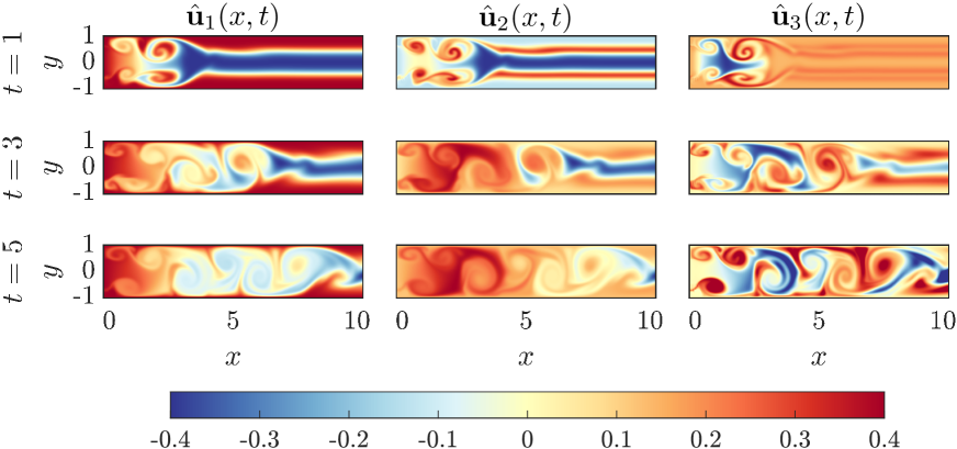
Figure 9: First three orthonormal f-OTD modes shown for r=8𝑟8r=8. Each row shows the modes at a different instance in time.

In Figure 9, the time-dependent evolution of the three most dominant f-OTD modes are shown. These modes are energetically ranked where low mode numbers correspond to larger (higher energy) structures and high mode numbers correspond to finer (lower energy) structures in the flow. As opposed to static basis, such as POD or DMD, the f-OTD modes evolve with the flow and exploit the instantaneous correlations between sensitivities. While this system is low-dimensional in the time-dependent basis, when expressed in POD or DMD basis, the system is high-dimensional and many modes are needed to capture the complex spatio-temporal evolution of 𝐕superscript𝐕\mathbf{V}^{\prime}. See reference [22] for comparison between time-dependent basis versus POD and DMD.
Refer to caption
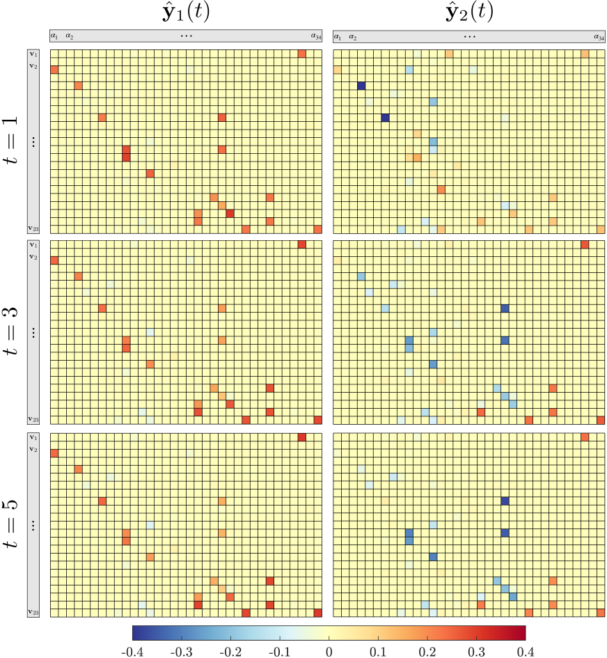
Figure 10: Orthonormalized f-OTD coefficients 𝐲^1(t)subscript^𝐲1𝑡\hat{\mathbf{y}}_{1}(t) and 𝐲^2(t)subscript^𝐲2𝑡\hat{\mathbf{y}}_{2}(t) visualized as a matrix with rows corresponding to species concentration and columns corresponding to reaction parameters. Color map shows most dominant sensitivities at different time instances.

To demonstrate the interpretability of the f-OTD decomposition, we show how the hidden parameter space represented by 𝐘^(t)^𝐘𝑡\hat{\mathbf{Y}}(t) can be used to identify the most important reaction parameters. In this context, importance refers to a parameter for which a small change in its value elicits a large change in the response of the system (i.e. highly sensitive). To demonstrate this capability of f-OTD, the first two sensitivity coefficients are visualized as matrices in Figure 10, where each 𝐲^isubscript^𝐲𝑖\hat{\mathbf{y}}_{i} is a d×1𝑑1d\times 1 vector that has been reshaped into an ns×nrsubscript𝑛𝑠subscript𝑛𝑟n_{s}\times n_{r} matrix. In this form, each 𝐯ijsubscriptsuperscript𝐯𝑖𝑗\mathbf{v}^{\prime}_{ij} is visualized using a heat map of the sensitivity coefficients, with rows corresponding to species i𝑖i and columns corresponding to reaction parameter j𝑗j. Using this heat map, Figure 10 shows that only a handful of sensitivities are non-zero, while the majority have zero contribution for the entire duration of the simulation.

4 Conclusions

We present a real time reduced order modeling approach for the computation of sensitivities in evolutionary systems governed by time dependent ordinary/partial differential equations. The computational cost of solving the f-OTD equations of rank r𝑟r is roughly equivalent to that of solving r𝑟r forward sensitivity equations. We demonstrated that the rank of f-OTD for two diverse applications is much smaller than the number of parameters. In contrast to adjoint based methods, f-OTD requires solving a system of forward equations and therefore it does not require any I/O operation. We showed that a single set of f-OTD modes can be formulated to compress the sensitivities of multi-variable PDEs. We demonstrated this capability by computing sensitivities of multiple species with respect to reaction parameters in a turbulent reactive flow.

In contrast to traditional ROM approaches, f-OTD extracts the low-rank approximation directly from the sensitivity equations as opposed to a data-driven approach, such as POD or DMD, which requires the full-dimensional sensitivity data. Moreover, the low-rank subspace in the data-driven approach is fine tuned to particular operating conditions, whereas the f-OTD subspace is evolved with the dynamics of the system and does not require such fine-tuning. As such, f-OTD is an on the fly model compression that is achieved by extracting instantaneous correlated structures in the solution.

Appendix A Optimality conditions of the variational principle

For the sake of brevity, we forgo the explicit written dependencies on x𝑥x, t𝑡t, and 𝜶𝜶\boldsymbol{\alpha} in the following derivation. Using index notation, we start by expanding 7

𝒢(𝐔˙,𝐘˙,λ)𝒢˙𝐔˙𝐘𝜆\displaystyle\mathcal{G}(\dot{\mathbf{U}},\dot{\mathbf{Y}},\lambda) =<𝐮˙i,𝐮˙j>(𝐲iT𝐲j)+<𝐮i,𝐮j>(𝐲˙iT𝐲˙j)+2<𝐮˙i,𝐮j>(𝐲iT𝐲˙j)\displaystyle=\big{<}\dot{\mathbf{u}}_{i},\dot{\mathbf{u}}_{j}\big{>}\left(\mathbf{y}_{i}^{T}\mathbf{y}_{j}\right)+\big{<}\mathbf{u}_{i},\mathbf{u}_{j}\big{>}\left(\dot{\mathbf{y}}_{i}^{T}\dot{\mathbf{y}}_{j}\right)+2\big{<}\dot{\mathbf{u}}_{i},\mathbf{u}_{j}\big{>}\left(\mathbf{y}_{i}^{T}\dot{\mathbf{y}}_{j}\right)
2<𝐮˙i,(𝐮j)>(𝐲iT𝐲j)2<𝐮i,(𝐮j)>(𝐲˙iT𝐲j)formulae-sequenceformulae-sequence2subscript˙𝐮𝑖subscript𝐮𝑗superscriptsubscript𝐲𝑖𝑇subscript𝐲𝑗2subscript𝐮𝑖subscript𝐮𝑗superscriptsubscript˙𝐲𝑖𝑇subscript𝐲𝑗\displaystyle-2\big{<}\dot{\mathbf{u}}_{i},\mathcal{L}(\mathbf{u}_{j})\big{>}\left(\mathbf{y}_{i}^{T}\mathbf{y}_{j}\right)-2\big{<}\mathbf{u}_{i},\mathcal{L}(\mathbf{u}_{j})\big{>}\left(\dot{\mathbf{y}}_{i}^{T}\mathbf{y}_{j}\right)
+<(𝐮i),(𝐮j)>(𝐲iT𝐲j)2<𝐮˙i,𝐅𝐲i>2<𝐮i,𝐅𝐲˙i>\displaystyle+\big{<}\mathcal{L}(\mathbf{u}_{i}),\mathcal{L}(\mathbf{u}_{j})\big{>}\left(\mathbf{y}_{i}^{T}\mathbf{y}_{j}\right)-2\big{<}\dot{\mathbf{u}}_{i},\mathbf{F}^{\prime}\mathbf{y}_{i}\big{>}-2\big{<}\mathbf{u}_{i},\mathbf{F}^{\prime}\dot{\mathbf{y}}_{i}\big{>}
+2<(𝐮i),𝐅𝐲i>+𝐅F2+λij(<𝐮i,𝐮˙j>ϕij).\displaystyle+2\big{<}\mathcal{L}(\mathbf{u}_{i}),\mathbf{F}^{\prime}\mathbf{y}_{i}\big{>}+\big{\|}\mathbf{F}^{\prime}\big{\|}_{F}^{2}+\lambda_{ij}\left(\big{<}\mathbf{u}_{i},\dot{\mathbf{u}}_{j}\big{>}-\phi_{ij}\right).

The first order optimality condition requires the derivative of 𝒢𝒢\mathcal{G} with respect to 𝐔˙,𝐘˙˙𝐔˙𝐘\dot{\mathbf{U}},\dot{\mathbf{Y}} and λ𝜆\lambda vanish. The derivative of 𝒢𝒢\mathcal{G} with respect to λ𝜆\lambda produces the time derivative of the orthonormality constraint given by Equation 6. Provided that the f-OTD modes are orthonormal at t=0𝑡0t=0, the time integration of Equation 6 reproduces the orthonormality condition of the f-OTD modes for t>0𝑡0t>0: <𝐮i,𝐮j>=δijformulae-sequenceabsentsubscript𝐮𝑖subscript𝐮𝑗subscript𝛿𝑖𝑗\big{<}\mathbf{u}_{i},\mathbf{u}_{j}\big{>}=\delta_{ij}. To take the derivative of 𝒢𝒢\mathcal{G} with respect to 𝐮˙~ksubscript~˙𝐮𝑘\tilde{\dot{\mathbf{u}}}_{k} we use the Fréchet differential as follows:

𝒢|𝐔˙limϵ0𝒢(𝐔˙+ϵ𝐔˙,𝐘˙,λ)𝒢(𝐔˙,𝐘˙,λ)ϵ.evaluated-atsuperscript𝒢˙𝐔subscriptitalic-ϵ0𝒢˙𝐔italic-ϵsuperscript˙𝐔˙𝐘𝜆𝒢˙𝐔˙𝐘𝜆italic-ϵ\mathcal{G}^{\prime}|_{\dot{\mathbf{U}}}\triangleq\lim_{\epsilon\rightarrow 0}\frac{\mathcal{G}(\dot{\mathbf{U}}+\epsilon\dot{\mathbf{U}}^{\prime},\dot{\mathbf{Y}},\lambda)-\mathcal{G}(\dot{\mathbf{U}},\dot{\mathbf{Y}},\lambda)}{\epsilon}.

Using the above definition we have:

𝒢|𝐮˙kevaluated-atsuperscript𝒢subscript˙𝐮𝑘\displaystyle\mathcal{G}^{\prime}|_{\dot{\mathbf{u}}_{k}} =2<𝐮˙,𝐮˙j>(𝐲kT𝐲j)+2<𝐮˙,𝐮j>(𝐲kT𝐲˙j)2<𝐮˙,(𝐮j)>(𝐲kT𝐲j)formulae-sequenceabsent2superscript˙𝐮subscript˙𝐮𝑗superscriptsubscript𝐲𝑘𝑇subscript𝐲𝑗2superscript˙𝐮subscript𝐮𝑗superscriptsubscript𝐲𝑘𝑇subscript˙𝐲𝑗2superscript˙𝐮subscript𝐮𝑗superscriptsubscript𝐲𝑘𝑇subscript𝐲𝑗\displaystyle=2\big{<}\dot{\mathbf{u}}^{\prime},\dot{\mathbf{u}}_{j}\big{>}\left(\mathbf{y}_{k}^{T}\mathbf{y}_{j}\right)+2\big{<}\dot{\mathbf{u}}^{\prime},\mathbf{u}_{j}\big{>}\left(\mathbf{y}_{k}^{T}\dot{\mathbf{y}}_{j}\right)-2\big{<}\dot{\mathbf{u}}^{\prime},\mathcal{L}(\mathbf{u}_{j})\big{>}\left(\mathbf{y}_{k}^{T}\mathbf{y}_{j}\right)
2<𝐮˙,𝐅𝐲k>+λjk<𝐮˙,𝐮j>=0.formulae-sequenceformulae-sequence2superscript˙𝐮superscript𝐅subscript𝐲𝑘subscript𝜆𝑗𝑘superscript˙𝐮subscript𝐮𝑗0\displaystyle-2\big{<}\dot{\mathbf{u}}^{\prime},\mathbf{F}^{\prime}\mathbf{y}_{k}\big{>}+\lambda_{jk}\big{<}\dot{\mathbf{u}}^{\prime},\mathbf{u}_{j}\big{>}=0.

The above equation can be written as <𝐮˙,𝐮˙k𝒢>\big{<}\dot{\mathbf{u}}^{\prime},\nabla_{\dot{\mathbf{u}}_{k}}\mathcal{G}\big{>} and we observe that for any arbitrary direction 𝐮˙superscript˙𝐮\dot{\mathbf{u}}^{\prime}, we must satisfy 𝐮˙k𝒢=𝟎subscriptsubscript˙𝐮𝑘𝒢0\nabla_{\dot{\mathbf{u}}_{k}}\mathcal{G}=\mathbf{0}. This leads to the following condition:

𝐮˙k𝒢=2𝐮˙j(𝐲kT𝐲j)+2𝐮j(𝐲kT𝐲˙j)2(𝐮j)(𝐲kT𝐲j)2𝐅𝐲k+λjk𝐮j=𝟎.subscriptsubscript˙𝐮𝑘𝒢2subscript˙𝐮𝑗superscriptsubscript𝐲𝑘𝑇subscript𝐲𝑗2subscript𝐮𝑗superscriptsubscript𝐲𝑘𝑇subscript˙𝐲𝑗2subscript𝐮𝑗superscriptsubscript𝐲𝑘𝑇subscript𝐲𝑗2superscript𝐅subscript𝐲𝑘subscript𝜆𝑗𝑘subscript𝐮𝑗0\nabla_{\dot{\mathbf{u}}_{k}}\mathcal{G}=2\dot{\mathbf{u}}_{j}\left(\mathbf{y}_{k}^{T}\mathbf{y}_{j}\right)+2\mathbf{u}_{j}\left(\mathbf{y}_{k}^{T}\dot{\mathbf{y}}_{j}\right)-2\mathcal{L}(\mathbf{u}_{j})\left(\mathbf{y}_{k}^{T}\mathbf{y}_{j}\right)-2\mathbf{F}^{\prime}\mathbf{y}_{k}+\lambda_{jk}\mathbf{u}_{j}=\mathbf{0}. (19)

To eliminate λjksubscript𝜆𝑗𝑘\lambda_{jk}, we take the inner product of 𝐮lsubscript𝐮𝑙\mathbf{u}_{l} with 19 to obtain

𝐮l,𝐮˙k𝒢subscript𝐮𝑙subscriptsubscript˙𝐮𝑘𝒢\displaystyle\left\langle\mathbf{u}_{l},\nabla_{\dot{\mathbf{u}}_{k}}\mathcal{G}\right\rangle =2ϕlj(𝐲kT𝐲j)+2δlj(𝐲kT𝐲˙j)2<𝐮l,(𝐮j)>(𝐲kT𝐲j)formulae-sequenceabsent2subscriptitalic-ϕ𝑙𝑗superscriptsubscript𝐲𝑘𝑇subscript𝐲𝑗2subscript𝛿𝑙𝑗superscriptsubscript𝐲𝑘𝑇subscript˙𝐲𝑗2subscript𝐮𝑙subscript𝐮𝑗superscriptsubscript𝐲𝑘𝑇subscript𝐲𝑗\displaystyle=2\phi_{lj}(\mathbf{y}_{k}^{T}\mathbf{y}_{j})+2\delta_{lj}\left(\mathbf{y}_{k}^{T}\dot{\mathbf{y}}_{j}\right)-2\big{<}\mathbf{u}_{l},\mathcal{L}(\mathbf{u}_{j})\big{>}\left(\mathbf{y}_{k}^{T}\mathbf{y}_{j}\right)
2<𝐮l,𝐅𝐲k>+λjkδlj=0,formulae-sequence2subscript𝐮𝑙superscript𝐅subscript𝐲𝑘subscript𝜆𝑗𝑘subscript𝛿𝑙𝑗0\displaystyle-2\big{<}\mathbf{u}_{l},\mathbf{F}^{\prime}\mathbf{y}_{k}\big{>}+\lambda_{jk}\delta_{lj}=0,

where we have used <𝐮l,𝐮˙j>=ϕljformulae-sequenceabsentsubscript𝐮𝑙subscript˙𝐮𝑗subscriptitalic-ϕ𝑙𝑗\big{<}\mathbf{u}_{l},\dot{\mathbf{u}}_{j}\big{>}=\phi_{lj} and <𝐮l,𝐮j>=δljformulae-sequenceabsentsubscript𝐮𝑙subscript𝐮𝑗subscript𝛿𝑙𝑗\big{<}\mathbf{u}_{l},\mathbf{u}_{j}\big{>}=\delta_{lj}. Rearranging for λlksubscript𝜆𝑙𝑘\lambda_{lk} gives

λlk=2[ϕlj(𝐲kT𝐲j)(𝐲kT𝐲˙l)+<𝐮l,(𝐮j)>(𝐲kT𝐲j)+<𝐮l,𝐅𝐲k>].\lambda_{lk}=2\left[-\phi_{lj}(\mathbf{y}_{k}^{T}\mathbf{y}_{j})-\left(\mathbf{y}_{k}^{T}\dot{\mathbf{y}}_{l}\right)+\big{<}\mathbf{u}_{l},\mathcal{L}(\mathbf{u}_{j})\big{>}\left(\mathbf{y}_{k}^{T}\mathbf{y}_{j}\right)+\big{<}\mathbf{u}_{l},\mathbf{F}^{\prime}\mathbf{y}_{k}\big{>}\right].

Dividing 19 by 2 and substituting λlksubscript𝜆𝑙𝑘\lambda_{lk} gives

[𝐮˙j(𝐮j)+<𝐮l,(𝐮j>)𝐮lϕlj𝐮l](𝐲kT𝐲j)𝐅𝐲k+<𝐮l,𝐅𝐲k>𝐮l=𝟎.\left[\dot{\mathbf{u}}_{j}-\mathcal{L}(\mathbf{u}_{j})+\big{<}\mathbf{u}_{l},\mathcal{L}(\mathbf{u}_{j}\big{>})\mathbf{u}_{l}-\phi_{lj}\mathbf{u}_{l}\right]\left(\mathbf{y}_{k}^{T}\mathbf{y}_{j}\right)-\mathbf{F}^{\prime}\mathbf{y}_{k}+\big{<}\mathbf{u}_{l},\mathbf{F}^{\prime}\mathbf{y}_{k}\big{>}\mathbf{u}_{l}=\mathbf{0}.

Rearranging the above equation for 𝐮˙jsubscript˙𝐮𝑗\dot{\mathbf{u}}_{j} we get

𝐮˙j=(𝐮j)<𝐮l,(𝐮j)>𝐮l+[𝐅𝐲k<𝐮l,𝐅𝐲k>𝐮l]Ckj1+ϕlj𝐮l,\boxed{\dot{\mathbf{u}}_{j}=\mathcal{L}(\mathbf{u}_{j})-\big{<}\mathbf{u}_{l},\mathcal{L}(\mathbf{u}_{j})\big{>}\mathbf{u}_{l}+\left[\mathbf{F}^{\prime}\mathbf{y}_{k}-\big{<}\mathbf{u}_{l},\mathbf{F}^{\prime}\mathbf{y}_{k}\big{>}\mathbf{u}_{l}\right]C_{kj}^{-1}+\phi_{lj}\mathbf{u}_{l},}

where Ckj=𝐲kT𝐲jsubscript𝐶𝑘𝑗superscriptsubscript𝐲𝑘𝑇subscript𝐲𝑗C_{kj}=\mathbf{y}_{k}^{T}\mathbf{y}_{j}. Similarly, the first order optimality condition of 𝒢𝒢\mathcal{G} with respect to 𝐲˙ksubscript˙𝐲𝑘\dot{\mathbf{y}}_{k} requires that

𝒢𝐲˙k=<𝐮k,𝐮j>𝐲˙j+<𝐮˙j,𝐮k>𝐲j<𝐮k,(𝐮j)>𝐲j<𝐅,𝐮k>=𝟎\displaystyle\dfrac{\partial\mathcal{G}}{\partial\dot{\mathbf{y}}_{k}}=\big{<}\mathbf{u}_{k},\mathbf{u}_{j}\big{>}\dot{\mathbf{y}}_{j}+\big{<}\dot{\mathbf{u}}_{j},\mathbf{u}_{k}\big{>}\mathbf{y}_{j}-\big{<}\mathbf{u}_{k},\mathcal{L}(\mathbf{u}_{j})\big{>}\mathbf{y}_{j}-\big{<}\mathbf{F}^{\prime},\mathbf{u}_{k}\big{>}=\mathbf{0}

Again, we use <𝐮k,𝐮j>=δkjformulae-sequenceabsentsubscript𝐮𝑘subscript𝐮𝑗subscript𝛿𝑘𝑗\big{<}\mathbf{u}_{k},\mathbf{u}_{j}\big{>}=\delta_{kj} and <𝐮˙j,𝐮k>=ϕjkformulae-sequenceabsentsubscript˙𝐮𝑗subscript𝐮𝑘subscriptitalic-ϕ𝑗𝑘\big{<}\dot{\mathbf{u}}_{j},\mathbf{u}_{k}\big{>}=-\phi_{jk}. Rearranging for 𝐲˙ksubscript˙𝐲𝑘\dot{\mathbf{y}}_{k} gives

𝐲˙k=<𝐮k,(𝐮j)>𝐲j+<𝐅,𝐮k>+ϕjk𝐲j.\boxed{\dot{\mathbf{y}}_{k}=\big{<}\mathbf{u}_{k},\mathcal{L}(\mathbf{u}_{j})\big{>}\mathbf{y}_{j}+\big{<}\mathbf{F}^{\prime},\mathbf{u}_{k}\big{>}+\phi_{jk}\mathbf{y}_{j}.}

Appendix B Equivalence of reductions

We prove the equivalence by using the evolution equation for the 𝐔,𝐘𝐔𝐘{\mathbf{U},\mathbf{Y}} and using the matrix differential equation for the rotation matrix 𝐑𝐑\mathbf{R} and recovering the evolution equations for 𝐔~,𝐘~~𝐔~𝐘{\tilde{\mathbf{U}},\tilde{\mathbf{Y}}}. To this end, we substitute 𝐔=𝐔~𝐑𝐔~𝐔𝐑\mathbf{U}=\tilde{\mathbf{U}}\mathbf{R} and 𝐘=𝐘~𝐑𝐘~𝐘𝐑\mathbf{Y}=\tilde{\mathbf{Y}}\mathbf{R} into the quasimatrix form of Equations 8 and 9. The evolution equation for the orthonormal modes becomes:

𝐔˙˙𝐔\displaystyle\dot{\mathbf{U}} =𝐔~˙𝐑+𝐔~𝐑˙absent˙~𝐔𝐑~𝐔˙𝐑\displaystyle=\dot{\tilde{\mathbf{U}}}\mathbf{R}+\tilde{\mathbf{U}}\dot{\mathbf{R}}
=(𝐔~)𝐑𝐔~𝐑<𝐔~𝐑,(𝐔~)𝐑>+[𝐅𝐘~𝐑𝐔~𝐑<𝐔~𝐑,𝐅𝐘~𝐑>]+𝐔~𝐑𝚽.\displaystyle=\mathcal{L}(\tilde{\mathbf{U}})\mathbf{R}-\tilde{\mathbf{U}}\mathbf{R}\big{<}\tilde{\mathbf{U}}\mathbf{R},\mathcal{L}(\tilde{\mathbf{U}})\mathbf{R}\big{>}+[\mathbf{F}^{\prime}\tilde{\mathbf{Y}}\mathbf{R}-\tilde{\mathbf{U}}\mathbf{R}\big{<}\tilde{\mathbf{U}}\mathbf{R},\mathbf{F}^{\prime}\tilde{\mathbf{Y}}\mathbf{R}\big{>}]+\tilde{\mathbf{U}}\mathbf{R}\boldsymbol{\Phi}.

Substituting 𝐑˙=𝐑𝚽𝚽~𝐑˙𝐑𝐑𝚽~𝚽𝐑\dot{\mathbf{R}}=\mathbf{R}\boldsymbol{\Phi}-\tilde{\boldsymbol{\Phi}}\mathbf{R} and solving for 𝐔~˙˙~𝐔\dot{\tilde{\mathbf{U}}} yields

𝐔~˙˙~𝐔\displaystyle\dot{\tilde{\mathbf{U}}} =[(𝐔~)𝐑𝐔~𝐑<𝐔~𝐑,(𝐔~)𝐑>+[𝐅𝐘~𝐑𝐔~𝐑<𝐔~𝐑,𝐅𝐘~𝐑>]\displaystyle=\big{[}\mathcal{L}(\tilde{\mathbf{U}})\mathbf{R}-\tilde{\mathbf{U}}\mathbf{R}\big{<}\tilde{\mathbf{U}}\mathbf{R},\mathcal{L}(\tilde{\mathbf{U}})\mathbf{R}\big{>}+[\mathbf{F}^{\prime}\tilde{\mathbf{Y}}\mathbf{R}-\tilde{\mathbf{U}}\mathbf{R}\big{<}\tilde{\mathbf{U}}\mathbf{R},\mathbf{F}^{\prime}\tilde{\mathbf{Y}}\mathbf{R}\big{>}]
+𝐔~𝐑𝚽𝐔~[𝐑𝚽𝚽~𝐑]𝐑T.~𝐔𝐑𝚽~𝐔delimited-[]𝐑𝚽~𝚽𝐑superscript𝐑𝑇\displaystyle+\tilde{\mathbf{U}}\mathbf{R}\boldsymbol{\Phi}-\tilde{\mathbf{U}}[\mathbf{R}\boldsymbol{\Phi}-\tilde{\boldsymbol{\Phi}}\mathbf{R}\big{]}\mathbf{R}^{T}.

Simplifying the above equation and using <𝐔~𝐑,>=𝐑T<𝐔~,>\big{<}\tilde{\mathbf{U}}\mathbf{R},\cdot\big{>}=\mathbf{R}^{T}\big{<}\tilde{\mathbf{U}},\cdot\big{>} and 𝐑1=𝐑Tsuperscript𝐑1superscript𝐑𝑇\mathbf{R}^{-1}=\mathbf{R}^{T}, since 𝐑𝐑\mathbf{R} is an orthonormal matrix results in:

𝐔~˙=(𝐔~)𝐔~<𝐔~,(𝐔~)>+[𝐅𝐘~𝐔~<𝐔~,𝐅𝐘~>]𝐂~1+𝐔~𝚽~,\displaystyle\dot{\tilde{\mathbf{U}}}=\mathcal{L}(\tilde{\mathbf{U}})-\tilde{\mathbf{U}}\big{<}\tilde{\mathbf{U}},\mathcal{L}(\tilde{\mathbf{U}})\big{>}+[\mathbf{F}^{\prime}\tilde{\mathbf{Y}}-\tilde{\mathbf{U}}\big{<}\tilde{\mathbf{U}},\mathbf{F}^{\prime}\tilde{\mathbf{Y}}\big{>}]\tilde{\mathbf{C}}^{-1}+\tilde{\mathbf{U}}\tilde{\boldsymbol{\Phi}},

where 𝐂~=𝐑𝐂𝐑T~𝐂superscript𝐑𝐂𝐑𝑇\tilde{\mathbf{C}}=\mathbf{R}\mathbf{C}\mathbf{R}^{T} and 𝐂~1=𝐑𝐂1𝐑Tsuperscript~𝐂1superscript𝐑𝐂1superscript𝐑𝑇\tilde{\mathbf{C}}^{-1}=\mathbf{R}\mathbf{C}^{-1}\mathbf{R}^{T}, where 𝐂𝐂\mathbf{C} and 𝐂~~𝐂\tilde{\mathbf{C}} are similar matrices and thus have the same eigenvalues. Following a similar procedure, the evolution equation for the coefficients becomes:

𝐘˙˙𝐘\displaystyle\dot{\mathbf{Y}} =𝐘~˙𝐑+𝐘~𝐑˙absent˙~𝐘𝐑~𝐘˙𝐑\displaystyle=\dot{\tilde{\mathbf{Y}}}\mathbf{R}+\tilde{\mathbf{Y}}\dot{\mathbf{R}}
=𝐘~𝐑<(𝐔~)𝐑,𝐔~>𝐑+<𝐅,𝐔~>𝐑+𝐘~𝐑𝚽.formulae-sequenceabsent~𝐘𝐑~𝐔𝐑~𝐔limit-from𝐑superscript𝐅~𝐔𝐑~𝐘𝐑𝚽\displaystyle=\tilde{\mathbf{Y}}\mathbf{R}\big{<}\mathcal{L}(\tilde{\mathbf{U}})\mathbf{R},\tilde{\mathbf{U}}\big{>}\mathbf{R}+\big{<}\mathbf{F}^{\prime},\tilde{\mathbf{U}}\big{>}\mathbf{R}+\tilde{\mathbf{Y}}\mathbf{R}\boldsymbol{\Phi}.

Substituting 𝐑˙=𝐑𝚽𝚽~𝐑˙𝐑𝐑𝚽~𝚽𝐑\dot{\mathbf{R}}=\mathbf{R}\boldsymbol{\Phi}-\tilde{\boldsymbol{\Phi}}\mathbf{R} and solving for 𝐘~˙˙~𝐘\dot{\tilde{\mathbf{Y}}} yields

𝐘~˙˙~𝐘\displaystyle\dot{\tilde{\mathbf{Y}}} =[𝐘~𝐑𝐑T<(𝐔~),𝐔~>𝐑+<𝐅,𝐔~>𝐑+𝐘~𝐑𝚽𝐘~[𝐑𝚽𝚽~𝐑]]𝐑T\displaystyle=\big{[}\tilde{\mathbf{Y}}\mathbf{R}\mathbf{R}^{T}\big{<}\mathcal{L}(\tilde{\mathbf{U}}),\tilde{\mathbf{U}}\big{>}\mathbf{R}+\big{<}\mathbf{F}^{\prime},\tilde{\mathbf{U}}\big{>}\mathbf{R}+\tilde{\mathbf{Y}}\mathbf{R}\boldsymbol{\Phi}-\tilde{\mathbf{Y}}[\mathbf{R}\boldsymbol{\Phi}-\tilde{\boldsymbol{\Phi}}\mathbf{R}]\big{]}\mathbf{R}^{T}
=𝐘~<(𝐔~),𝐔~>+<𝐅,𝐔~>+𝐘~𝚽~.\displaystyle=\tilde{\mathbf{Y}}\big{<}\mathcal{L}(\tilde{\mathbf{U}}),\tilde{\mathbf{U}}\big{>}+\big{<}\mathbf{F}^{\prime},\tilde{\mathbf{U}}\big{>}+\tilde{\mathbf{Y}}\tilde{\boldsymbol{\Phi}}.

Thus, we have shown that the evolution of {𝐔(x,t),𝐘(t)}𝐔𝑥𝑡𝐘𝑡\{\mathbf{U}(x,t),\mathbf{Y}(t)\} and {𝐔~(x,t),𝐘~(t)}~𝐔𝑥𝑡~𝐘𝑡\{\tilde{\mathbf{U}}(x,t),\tilde{\mathbf{Y}}(t)\} according to Equations 8 and 9 are equivalent.

Appendix C Exactness of f-OTD

Start by substituting 𝐕(x,t)=𝐔(x,t)𝐘(t)Tsuperscript𝐕𝑥𝑡𝐔𝑥𝑡𝐘superscript𝑡𝑇\mathbf{V}^{\prime}(x,t)=\mathbf{U}(x,t)\mathbf{Y}(t)^{T} into the quasimatrix form of Equation 3:

𝐔˙𝐘T+𝐔𝐘˙T=(𝐔)𝐘T+𝐅.˙𝐔superscript𝐘𝑇𝐔superscript˙𝐘𝑇𝐔superscript𝐘𝑇superscript𝐅\displaystyle\dot{\mathbf{U}}\mathbf{Y}^{T}+\mathbf{U}\dot{\mathbf{Y}}^{T}=\mathcal{L}(\mathbf{U})\mathbf{Y}^{T}+\mathbf{F}^{\prime}.

Next we substitute 𝐘˙Tsuperscript˙𝐘𝑇\dot{\mathbf{Y}}^{T} from Equation 9

𝐔˙𝐘T+𝐔(𝐋r𝐘T+<𝐔,𝐅>)=(𝐔)𝐘T+𝐅,\dot{\mathbf{U}}\mathbf{Y}^{T}+\mathbf{U}\left(\mathbf{L}_{r}\mathbf{Y}^{T}+\big{<}\mathbf{U},\mathbf{F}^{\prime}\big{>}\right)=\mathcal{L}(\mathbf{U})\mathbf{Y}^{T}+\mathbf{F}^{\prime},

where we have used 𝐋r(t)=<𝐔(x,t),(𝐔(x,t))>\mathbf{L}_{r}(t)=\big{<}\mathbf{U}(x,t),\mathcal{L}(\mathbf{U}(x,t))\big{>}. We multiply by 𝐘𝐘\mathbf{Y} from right and rearrange to get

𝐔˙𝐂=(𝐔)𝐂𝐔𝐋r𝐂+(𝐅𝐘𝐔<𝐔,𝐅𝐘>),\dot{\mathbf{U}}\mathbf{C}=\mathcal{L}(\mathbf{U})\mathbf{C}-\mathbf{U}\mathbf{L}_{r}\mathbf{C}+\left(\mathbf{F}^{\prime}\mathbf{Y}-\mathbf{U}\big{<}\mathbf{U},\mathbf{F}^{\prime}\mathbf{Y}\big{>}\right),

where we have used 𝐂=𝐘T𝐘𝐂superscript𝐘𝑇𝐘\mathbf{C}=\mathbf{Y}^{T}\mathbf{Y}. Finally, we multiply by 𝐂1superscript𝐂1\mathbf{C}^{-1} from right to get

𝐔˙=(𝐔)𝐔𝐋r+(𝐅𝐘𝐔<𝐔,𝐅𝐘>)𝐂1,\dot{\mathbf{U}}=\mathcal{L}(\mathbf{U})-\mathbf{U}\mathbf{L}_{r}+\left(\mathbf{F}^{\prime}\mathbf{Y}-\mathbf{U}\big{<}\mathbf{U},\mathbf{F}^{\prime}\mathbf{Y}\big{>}\right)\mathbf{C}^{-1},

which is the same as the evolution Equation 8 for the orthonormal basis. Here we have shown that the evolution of 𝐕(x,t)superscript𝐕𝑥𝑡\mathbf{V}^{\prime}(x,t) under Equation 3 is equivalent to the evolution of 𝐔(x,t)𝐔𝑥𝑡\mathbf{U}(x,t) under Equation 8. That is, when r=d𝑟𝑑r=d, 𝐘(t)T𝐘superscript𝑡𝑇\mathbf{Y}(t)^{T} is a linear transformation that exactly maps the orthonormal subspace 𝐔(x,t)𝐔𝑥𝑡\mathbf{U}(x,t) to 𝐕(x,t)superscript𝐕𝑥𝑡\mathbf{V}^{\prime}(x,t).

Appendix D f-OTD Derivation for Tensor Sensitivities

We start by considering the third order quasitensor 𝐕~=[𝐯~ij]×ns×nrsuperscript~𝐕delimited-[]subscriptsuperscript~𝐯𝑖𝑗superscriptsubscript𝑛𝑠subscript𝑛𝑟\tilde{\mathbf{V}}^{\prime}=[\tilde{\mathbf{v}}^{\prime}_{ij}]\in\mathbb{R}^{\infty\times n_{s}\times n_{r}} that we seek to flatten into a quasimatrix 𝐕=[𝐯m]×dsuperscript𝐕delimited-[]subscriptsuperscript𝐯𝑚superscript𝑑\mathbf{V}^{\prime}=[\mathbf{v}^{\prime}_{m}]\in\mathbb{R}^{\infty\times d}. For ease of reference, we rewrite the tensor evolution Equation 17 below:

𝐯~ijt+(𝐮)𝐯~ij=κ~ik2𝐯~kj+~𝐬ik𝐯~kj+𝐬~ij,superscriptsubscript~𝐯𝑖𝑗𝑡𝐮superscriptsubscript~𝐯𝑖𝑗subscript~𝜅𝑖𝑘superscript2superscriptsubscript~𝐯𝑘𝑗subscript~subscript𝐬𝑖𝑘superscriptsubscript~𝐯𝑘𝑗subscriptsuperscript~𝐬𝑖𝑗\dfrac{\partial\tilde{\mathbf{v}}_{ij}^{\prime}}{\partial t}+\left(\mathbf{u}\cdot\nabla\right)\tilde{\mathbf{v}}_{ij}^{\prime}=\tilde{\kappa}_{ik}\nabla^{2}\tilde{\mathbf{v}}_{kj}^{\prime}+\tilde{\mathcal{L}}_{\mathbf{s}_{ik}}\tilde{\mathbf{v}}_{kj}^{\prime}+\tilde{\mathbf{s}}^{\prime}_{ij},

where i,k=1,2,,nsformulae-sequence𝑖𝑘12subscript𝑛𝑠i,k=1,2,\dots,n_{s} and j=1,2,,nr𝑗12subscript𝑛𝑟j=1,2,\dots,n_{r}. We define the indices m(i,j)=j+(i1)nr𝑚𝑖𝑗𝑗𝑖1subscript𝑛𝑟m(i,j)=j+(i-1)n_{r} and n(i,j)=j+(i1)nr𝑛superscript𝑖superscript𝑗superscript𝑗superscript𝑖1subscript𝑛𝑟n(i^{\prime},j^{\prime})=j^{\prime}+(i^{\prime}-1)n_{r}, where i=1,2,,nssuperscript𝑖12subscript𝑛𝑠i^{\prime}=1,2,\dots,n_{s} and j=1,2,,nrsuperscript𝑗12subscript𝑛𝑟j^{\prime}=1,2,\dots,n_{r}. In the above equation, the terms 𝐯~ijsuperscriptsubscript~𝐯𝑖𝑗\tilde{\mathbf{v}}_{ij}^{\prime} and 𝐬~ijsubscriptsuperscript~𝐬𝑖𝑗\tilde{\mathbf{s}}^{\prime}_{ij} are flattened by replacing the index pair ij𝑖𝑗ij with the single index m𝑚m: 𝐯m(i,j)=𝐯~ijsubscriptsuperscript𝐯𝑚𝑖𝑗superscriptsubscript~𝐯𝑖𝑗\mathbf{v}^{\prime}_{m(i,j)}=\tilde{\mathbf{v}}_{ij}^{\prime} and 𝐬m(i,j)=𝐬~ijsubscriptsuperscript𝐬𝑚𝑖𝑗superscriptsubscript~𝐬𝑖𝑗\mathbf{s}^{\prime}_{m(i,j)}=\tilde{\mathbf{s}}_{ij}^{\prime}. Next, we define a new diffusion coefficient matrix κmnd×dsubscript𝜅𝑚𝑛superscript𝑑𝑑\kappa_{mn}\in\mathbb{R}^{d\times d} such that the m𝑚mth diagonal entry is equal the diffusion coefficient of the i𝑖ith species. That is, κmnsubscript𝜅𝑚𝑛\kappa_{mn} is independent of parameter index j𝑗j and remains constant across all sensitivities of a given species i𝑖i. Finally, the linearized reactive source term is defined as 𝐬m(i,j)n(i,j)=~𝐬iiδjjsubscriptsubscript𝐬𝑚𝑖𝑗𝑛superscript𝑖superscript𝑗subscript~subscript𝐬𝑖superscript𝑖subscript𝛿𝑗superscript𝑗\mathcal{L}_{\mathbf{s}_{m(i,j)n(i^{\prime},j^{\prime})}}=\tilde{\mathcal{L}}_{\mathbf{s}_{ii^{\prime}}}\delta_{jj^{\prime}}, where δjjsubscript𝛿𝑗superscript𝑗\delta_{jj^{\prime}} is the Kronecker delta and n𝑛n is a dummy index corresponding to 𝐯nsubscriptsuperscript𝐯𝑛\mathbf{v}^{\prime}_{n}. From this definition, δjjsubscript𝛿𝑗superscript𝑗\delta_{jj^{\prime}} results in non-zero contribution to the summation over n𝑛n only for sensitivities with respect to parameter j=jsuperscript𝑗𝑗j^{\prime}=j. Putting this all together, the above equation can be written as:

𝐯mt+(𝐰)𝐯m=κmn2𝐯n+𝐬mn𝐯n+𝐬m,subscriptsuperscript𝐯𝑚𝑡𝐰subscriptsuperscript𝐯𝑚subscript𝜅𝑚𝑛superscript2subscriptsuperscript𝐯𝑛subscriptsubscript𝐬𝑚𝑛subscriptsuperscript𝐯𝑛subscriptsuperscript𝐬𝑚\dfrac{\partial\mathbf{v}^{\prime}_{m}}{\partial t}+(\mathbf{w}\cdot\nabla)\mathbf{v}^{\prime}_{m}=\kappa_{mn}\nabla^{2}\mathbf{v}^{\prime}_{n}+\mathcal{L}_{\mathbf{s}_{mn}}\mathbf{v}^{\prime}_{n}+\mathbf{s}^{\prime}_{m}, (20)

where 𝐬mn𝐯nsubscriptsubscript𝐬𝑚𝑛subscriptsuperscript𝐯𝑛\mathcal{L}_{\mathbf{s}_{mn}}\mathbf{v}^{\prime}_{n} should be interpreted as a matrix-vector multiplication for any (x1,x2)subscript𝑥1subscript𝑥2(x_{1},x_{2}) point in the physical space. As a result of the parametric dependence of the linear operator, Equations 8 and 9 do not hold for the tensor flattened equation. Therefore, we must derive new evolution equations for the f-OTD modes and coefficients for tensor flattened quantities. Substituting the approximation 𝐯m=i=1r𝐮iYmisubscriptsuperscript𝐯𝑚superscriptsubscript𝑖1𝑟subscript𝐮𝑖subscript𝑌𝑚𝑖\mathbf{v}^{\prime}_{m}=\sum_{i=1}^{r}\mathbf{u}_{i}Y_{mi} into the above equation, it is straightforward to show that the evolution equations for the f-OTD modes and coefficients are:

𝐮˙i=subscript˙𝐮𝑖absent\displaystyle\dot{\mathbf{u}}_{i}= [(𝐰)𝐮i𝐮j<𝐮j,(𝐰)𝐮i>]+[2𝐮k𝐮j<𝐮j,2𝐮k>]YnkκmnYmlCil1\displaystyle-\left[(\mathbf{w}\cdot\nabla)\mathbf{u}_{i}-\mathbf{u}_{j}\big{<}\mathbf{u}_{j},(\mathbf{w}\cdot\nabla)\mathbf{u}_{i}\big{>}\right]+\left[\nabla^{2}\mathbf{u}_{k}-\mathbf{u}_{j}\big{<}\mathbf{u}_{j},\nabla^{2}\mathbf{u}_{k}\big{>}\right]Y_{nk}\kappa_{mn}Y_{ml}C^{-1}_{il}
+[𝐬mn𝐮k𝐮j<𝐮j,𝐬mn𝐮k>]YnkYmlCil1+[𝐬m𝐮j<𝐮j,𝐬m>]YmlCil1,\displaystyle+\left[\mathcal{L}_{\mathbf{s}_{mn}}\mathbf{u}_{k}-\mathbf{u}_{j}\big{<}\mathbf{u}_{j},\mathcal{L}_{\mathbf{s}_{mn}}\mathbf{u}_{k}\big{>}\right]Y_{nk}Y_{ml}C^{-1}_{il}+\left[\mathbf{s}^{\prime}_{m}-\mathbf{u}_{j}\big{<}\mathbf{u}_{j},\mathbf{s}^{\prime}_{m}\big{>}\right]Y_{ml}C^{-1}_{il}, (21)

and

Y˙mj=subscript˙𝑌𝑚𝑗absent\displaystyle\dot{Y}_{mj}= <𝐮j,(𝐰)𝐮i>Ymi+<𝐮j,2𝐮i>Yniκmn\displaystyle-\big{<}\mathbf{u}_{j},(\mathbf{w}\cdot\nabla)\mathbf{u}_{i}\big{>}Y_{mi}+\big{<}\mathbf{u}_{j},\nabla^{2}\mathbf{u}_{i}\big{>}Y_{ni}\kappa_{mn}
+<𝐮j,𝐬mn𝐮i>Yni+<𝐮j,𝐬m>,\displaystyle+\big{<}\mathbf{u}_{j},\mathcal{L}_{\mathbf{s}_{mn}}\mathbf{u}_{i}\big{>}Y_{ni}+\big{<}\mathbf{u}_{j},\mathbf{s}^{\prime}_{m}\big{>}, (22)

where 𝐘=[Ymi]𝐘delimited-[]subscript𝑌𝑚𝑖\mathbf{Y}=[Y_{mi}] and the indices m,n=1,2,,dformulae-sequence𝑚𝑛12𝑑m,n=1,2,\dots,d and i,j,k=1,2,,rformulae-sequence𝑖𝑗𝑘12𝑟i,j,k=1,2,\dots,r.

Appendix E Reactive source term specification

𝐬1=(α1[13][2])/(α2+[2])α3[1][15]subscript𝐬1subscript𝛼1delimited-[]13delimited-[]2subscript𝛼2delimited-[]2subscript𝛼3delimited-[]1delimited-[]15\mathbf{s}_{1}=(\alpha_{1}[13][2])/(\alpha_{2}+[2])-\alpha_{3}[1][15]
𝐬2=(α1[13][2]/(α2+[2])\mathbf{s}_{2}=-(\alpha_{1}[13][2]/(\alpha_{2}+[2])
𝐬3=(α4[9][4]/(α5+[4])α6[3](α7[17][3])/(α8+[3])\mathbf{s}_{3}=(\alpha_{4}[9][4]/(\alpha_{5}+[4])-\alpha_{6}[3]-(\alpha_{7}[17][3])/(\alpha_{8}+[3])
𝐬4=(α4[9][4])/(α5+[4])subscript𝐬4subscript𝛼4delimited-[]9delimited-[]4subscript𝛼5delimited-[]4\mathbf{s}_{4}=(\alpha_{4}[9][4])/(\alpha_{5}+[4])
𝐬5=(α9[9][6])/(α10+[6])α11[5](α12[17][5])/(α13+[5])subscript𝐬5subscript𝛼9delimited-[]9delimited-[]6subscript𝛼10delimited-[]6subscript𝛼11delimited-[]5subscript𝛼12delimited-[]17delimited-[]5subscript𝛼13delimited-[]5\mathbf{s}_{5}=(\alpha_{9}[9][6])/(\alpha_{10}+[6])-\alpha_{11}[5]-(\alpha_{12}[17][5])/(\alpha_{13}+[5])
𝐬6=(α9[9][6]/(α10+[6])\mathbf{s}_{6}=-(\alpha_{9}[9][6]/(\alpha_{10}+[6])
𝐬7=(α14[24][8])/(α15+[8])α16[7][15]α17[16][7]subscript𝐬7subscript𝛼14delimited-[]24delimited-[]8subscript𝛼15delimited-[]8subscript𝛼16delimited-[]7delimited-[]15subscript𝛼17delimited-[]16delimited-[]7\mathbf{s}_{7}=(\alpha_{14}[24][8])/(\alpha_{15}+[8])-\alpha_{16}[7][15]-\alpha_{17}[16][7]
𝐬8=(α14[24][8])/(α15+[8])subscript𝐬8subscript𝛼14delimited-[]24delimited-[]8subscript𝛼15delimited-[]8\mathbf{s}_{8}=-(\alpha_{14}[24][8])/(\alpha_{15}+[8])
𝐬9=(α18[25][10])/(α19+[10])α20[9][15]subscript𝐬9subscript𝛼18delimited-[]25delimited-[]10subscript𝛼19delimited-[]10subscript𝛼20delimited-[]9delimited-[]15\mathbf{s}_{9}=(\alpha_{18}[25][10])/(\alpha_{19}+[10])-\alpha_{20}[9][15]
𝐬10=(α18[25][10])/(α19+[10])subscript𝐬10subscript𝛼18delimited-[]25delimited-[]10subscript𝛼19delimited-[]10\mathbf{s}_{10}=-(\alpha_{18}[25][10])/(\alpha_{19}+[10])
𝐬11=(α21[9][12])/(α22+[12])(α23[21][11])/(α24+[11])subscript𝐬11subscript𝛼21delimited-[]9delimited-[]12subscript𝛼22delimited-[]12subscript𝛼23delimited-[]21delimited-[]11subscript𝛼24delimited-[]11\mathbf{s}_{11}=(\alpha_{21}[9][12])/(\alpha_{22}+[12])-(\alpha_{23}[21][11])/(\alpha_{24}+[11])
𝐬12=(α21[9][12])/(α22+[12])subscript𝐬12subscript𝛼21delimited-[]9delimited-[]12subscript𝛼22delimited-[]12\mathbf{s}_{12}=-(\alpha_{21}[9][12])/(\alpha_{22}+[12])
𝐬13=(α25[9][14])/(α26+[14])α27[13][15]α28[13][19]subscript𝐬13subscript𝛼25delimited-[]9delimited-[]14subscript𝛼26delimited-[]14subscript𝛼27delimited-[]13delimited-[]15subscript𝛼28delimited-[]13delimited-[]19\mathbf{s}_{13}=(\alpha_{25}[9][14])/(\alpha_{26}+[14])-\alpha_{27}[13][15]-\alpha_{28}[13][19]
𝐬14=(α25[9][14])/(α26+[14])subscript𝐬14subscript𝛼25delimited-[]9delimited-[]14subscript𝛼26delimited-[]14\mathbf{s}_{14}=-(\alpha_{25}[9][14])/(\alpha_{26}+[14])
𝐬15=(α3[1]+α16[7]+α20[9]+α27[13])[15]subscript𝐬15subscript𝛼3delimited-[]1subscript𝛼16delimited-[]7subscript𝛼20delimited-[]9subscript𝛼27delimited-[]13delimited-[]15\mathbf{s}_{15}=-(\alpha_{3}[1]+\alpha_{16}[7]+\alpha_{20}[9]+\alpha_{27}[13])[15]
𝐬16=α17[16][7]subscript𝐬16subscript𝛼17delimited-[]16delimited-[]7\mathbf{s}_{16}=-\alpha_{17}[16][7]
𝐬17=(α29[9][18])/(α30+[18])α31[17][19]subscript𝐬17subscript𝛼29delimited-[]9delimited-[]18subscript𝛼30delimited-[]18subscript𝛼31delimited-[]17delimited-[]19\mathbf{s}_{17}=(\alpha_{29}[9][18])/(\alpha_{30}+[18])-\alpha_{31}[17][19]
𝐬18=(α29[9][18](α30+[18])\mathbf{s}_{18}=-(\alpha_{29}[9][18](\alpha_{30}+[18])
𝐬19=α31[17][19]α28[13][19]subscript𝐬19subscript𝛼31delimited-[]17delimited-[]19subscript𝛼28delimited-[]13delimited-[]19\mathbf{s}_{19}=-\alpha_{31}[17][19]-\alpha_{28}[13][19]
𝐬20=0subscript𝐬200\mathbf{s}_{20}=0
𝐬21=(α32[20][22])/(α33+[22])α34[21][23]subscript𝐬21subscript𝛼32delimited-[]20delimited-[]22subscript𝛼33delimited-[]22subscript𝛼34delimited-[]21delimited-[]23\mathbf{s}_{21}=(\alpha_{32}[20][22])/(\alpha_{33}+[22])-\alpha_{34}[21][23]
𝐬22=(α32[20][22])/(α33+[22])subscript𝐬22subscript𝛼32delimited-[]20delimited-[]22subscript𝛼33delimited-[]22\mathbf{s}_{22}=-(\alpha_{32}[20][22])/(\alpha_{33}+[22])
𝐬23=α34[21][23]subscript𝐬23subscript𝛼34delimited-[]21delimited-[]23\mathbf{s}_{23}=-\alpha_{34}[21][23]
Table 1: Reactive source terms with species concentration denoted by []delimited-[][\cdot]. Each 𝐬isubscript𝐬𝑖\mathbf{s}_{i} is scaled by 102superscript10210^{2} for time scale adjustment with the flow and the parameter values are assigned as follows: α1=2.54×10²subscript𝛼12.54superscript102\alpha_{1}=2.54\times 10^{-2}, α2=160subscript𝛼2160\alpha_{2}=160, α3=3.74×10⁵subscript𝛼33.74superscript105\alpha_{3}=3.74\times 10^{-5}, α4=0.449subscript𝛼40.449\alpha_{4}=0.449, α5=1.12×10⁵subscript𝛼51.12superscript105\alpha_{5}=1.12\times 10^{5}, α6=5.13×10⁴subscript𝛼65.13superscript104\alpha_{6}=5.13\times 10^{-4}, α7=2.36×10²subscript𝛼72.36superscript102\alpha_{7}=2.36\times 10^{-2}, α8=14.6subscript𝛼814.6\alpha_{8}=14.6, α9=6.24×10²subscript𝛼96.24superscript102\alpha_{9}=6.24\times 10^{-2}, α10=140.5subscript𝛼10140.5\alpha_{10}=140.5, α11=3.93×10⁴subscript𝛼113.93superscript104\alpha_{11}=3.93\times 10^{-4}, α12=2.36×10²subscript𝛼122.36superscript102\alpha_{12}=2.36\times 10^{-2}, α13=14.6subscript𝛼1314.6\alpha_{13}=14.6, α14=5.523subscript𝛼145.523\alpha_{14}=5.523, α15=160subscript𝛼15160\alpha_{15}=160, α16=8.01×10⁴subscript𝛼168.01superscript104\alpha_{16}=8.01\times 10^{-4}, α17=1.11×10³subscript𝛼171.11superscript103\alpha_{17}=1.11\times 10^{-3}, α18=3.105subscript𝛼183.105\alpha_{18}=3.105, α19=1060subscript𝛼191060\alpha_{19}=1060, α20=1.65×10³subscript𝛼201.65superscript103\alpha_{20}=1.65\times 10^{-3}, α21=8.177subscript𝛼218.177\alpha_{21}=8.177, α22=3160subscript𝛼223160\alpha_{22}=3160, α23=3.456subscript𝛼233.456\alpha_{23}=3.456, α24=2.50×10⁵subscript𝛼242.50superscript105\alpha_{24}=2.50\times 10^{5}, α25=1.80×10⁵subscript𝛼251.80superscript105\alpha_{25}=1.80\times 10^{-5}, α26=50subscript𝛼2650\alpha_{26}=50, α27=3.70×10⁶subscript𝛼273.70superscript106\alpha_{27}=3.70\times 10^{-6}, α28=3.00×10⁸subscript𝛼283.00superscript108\alpha_{28}=3.00\times 10^{-8}, α29=9.01×10²subscript𝛼299.01superscript102\alpha_{29}=9.01\times 10^{-2}, α30=3190subscript𝛼303190\alpha_{30}=3190, α31=1.52×10⁹subscript𝛼311.52superscript109\alpha_{31}=1.52\times 10^{-9}, α32=2.77×10²subscript𝛼322.77superscript102\alpha_{32}=2.77\times 10^{-2}, α33=18subscript𝛼3318\alpha_{33}=18, and α34=2.22×10⁴subscript𝛼342.22superscript104\alpha_{34}=2.22\times 10^{-4}

Acknowledgments

We gratefully acknowledge the support received from the NASA Transformational Tools and Technologies Project, grant no. 80NSSC18M0150. We would also like to thank Dr. Joseph Derlaga for his support and intellectual insight throughout the process.

References

  • [1] Michael B. Giles and Niles A. Pierce. An introduction to the adjoint approach to design. Flow, Turbulence and Combustion, 65(3):393–415, 2000.
  • [2] M.D. Gunzburger. Sensitivities, adjoints and flow optimization. International Journal for Numerical Methods in Fluids, 31(1):53–78, 1999.
  • [3] T.R. Bewley, P. Moin, and R. Temam. DNS-based predictive control of turbulence: an optimal benchmark for feedback algorithms. 447:179–225, 2001.
  • [4] K. T. Doetsch and K. J. Fidkowski. Combined entropy and output-based adjoint approach for mesh refinement and error estimation. AIAA Journal, 57(8):3213–3230, 2020/10/26 2019.
  • [5] G. Esposito and H. K. Chelliah. Skeletal reaction models based on principal component analysis: Application to ethylene–air ignition, propagation, and extinction phenomena. Combustion and Flame, 158(3):477–489, 2011.
  • [6] Applied mathematics research for exascale computing. U.S. Department of Energy, Office of Science, Advanced Scientific Computing Research Program, 2014.
  • [7] J. C. Bennett, H. Abbasi, P. Bremer, R. Grout, A. Gyulassy, T. Jin, S. Klasky, H. Kolla, M. Parashar, V. Pascucci, P. Pebay, D. Thompson, H. Yu, F. Zhang, and J. Chen. Combining in-situ and in-transit processing to enable extreme-scale scientific analysis. In SC ’12: Proceedings of the International Conference on High Performance Computing, Networking, Storage and Analysis, pages 1–9, 2012.
  • [8] H. Babaee and T. P. Sapsis. A minimization principle for the description of modes associated with finite-time instabilities. Proceedings of the Royal Society of London A: Mathematical, Physical and Engineering Sciences, 472(2186), 2016.
  • [9] H. Babaee, M. Farazmand, G. Haller, and T. P. Sapsis. Reduced-order description of transient instabilities and computation of finite-time Lyapunov exponents. Chaos: An Interdisciplinary Journal of Nonlinear Science, 27(6):063103, 2017/06/11 2017.
  • [10] A. Blanchard, S. Mowlavi, and T. Sapsis. Control of linear instabilities by dynamically consistent order reduction on optimally time-dependent modes. Nonlinear Dynamics, In press, 2018.
  • [11] Mohammad Farazmand and Themistoklis P. Sapsis. Dynamical indicators for the prediction of bursting phenomena in high-dimensional systems. Phys. Rev. E, 94:032212, Sep 2016.
  • [12] M. Beneitez, Y. Duguet, P. Schlatter, and D. S. Henningson. Edge manifold as a lagrangian coherent structure in a high-dimensional state space. Physical Review Research, 2(3):033258–, 08 2020.
  • [13] T.P. Sapsis and P.F.J. Lermusiaux. Dynamically orthogonal field equations for continuous stochastic dynamical systems. Physica D: Nonlinear Phenomena, 238(23-24):2347–2360, 2009.
  • [14] M. Cheng, T. Y. Hou, and Z. Zhang. A dynamically bi-orthogonal method for time-dependent stochastic partial differential equations i: Derivation and algorithms. Journal of Computational Physics, 242(0):843 – 868, 2013.
  • [15] E. Musharbash, F. Nobile, and T. Zhou. Error analysis of the dynamically orthogonal approximation of time dependent random pdes. SIAM Journal on Scientific Computing, 37(2):A776–A810, 2018/01/17 2015.
  • [16] H. Babaee, M. Choi, T. P. Sapsis, and G. E. Karniadakis. A robust bi-orthogonal/dynamically-orthogonal method using the covariance pseudo-inverse with application to stochastic flow problems. Journal of Computational Physics, 344:303–319, 9 2017.
  • [17] P. Patil and H. Babaee. Real-time reduced-order modeling of stochastic partial differential equations via time-dependent subspaces. Journal of Computational Physics, 415:109511, 2020.
  • [18] K. Braman, To. A. Oliver, and V. Raman. Adjoint-based sensitivity analysis of flames. Combustion Theory and Modelling, 19(1):29–56, 01 2015.
  • [19] M. Lemke, L. Cai, J. Reiss, H. Pitsch, and J. Sesterhenn. Adjoint-based sensitivity analysis of quantities of interest of complex combustion models. Combustion Theory and Modelling, 23(1):180–196, 01 2019.
  • [20] R. Langer, J. Lotz, L. Cai, F. vom Lehn, K. Leppkes, U. Naumann, and H. Pitsch. Adjoint sensitivity analysis of kinetic, thermochemical, and transport data of nitrogen and ammonia chemistry. Proceedings of the Combustion Institute, 2020.
  • [21] Z. Battles and L. Trefethen. An extension of matlab to continuous functions and operators. SIAM Journal on Scientific Computing, 25(5):1743–1770, 2004.
  • [22] H. Babaee. An observation-driven time-dependent basis for a reduced description of transient stochastic systems. Proceedings of the Royal Society A: Mathematical, Physical and Engineering Sciences, 475(2231):20190506, 2019.
  • [23] N. Aubry. On the hidden beauty of the proper orthogonal decomposition. 2(5-6):339–352, 1991.
  • [24] L. Alvergue, H. Babaee, G. Gu, and S. Acharya. Feedback stabilization of a reduced-order model of a jet in crossflow. AIAA Journal, 53(9):2472–2481, 2016/02/17 2015.
  • [25] P. Arrué, N. Toosizadeh, H. Babaee, and K. Laksari. Low-rank representation of head impact kinematics: A data-driven emulator. Frontiers in Bioengineering and Biotechnology, 8:1049, 2020.
  • [26] P.J. Schmid. Dynamic mode decomposition of numerical and experimental data. Journal of Fluid Mechanics, 656:5–28, 2010.
  • [27] K. Laksari, M. Kurt, H. Babaee, S. Kleiven, and D. Camarillo. Mechanistic insights into human brain impact dynamics through modal analysis. Physical Review Letters, 120(13):138101–, 03 2018.
  • [28] O. Koch and C. Lubich. Dynamical low-rank approximation. SIAM Journal on Matrix Analysis and Applications, 29(2):434–454, 2017/04/02 2007.
  • [29] A. J. Chorin, O. H. Hald, and R. Kupferman. Optimal prediction with memory. Physica D: Nonlinear Phenomena, 166(3–4):239 – 257, 2002.
  • [30] D. Ruelle. Differentiation of srb states. Communications in Mathematical Physics, 187(1):227–241, 1997.
  • [31] Eyink G. L., T. W. N. Haine, and D. J. Lea. Ruelle’s linear response formula, ensemble adjoint schemes and lévy flights. Nonlinearity, 17(5):1867, 2004.
  • [32] Aly-Khan. Kassam and Lloyd N. Trefethen. Fourth-order time-stepping for stiff pdes. SIAM Journal on Scientific Computing, 26(4):1214–1233, 2019/12/23 2005.
  • [33] Z. Li, A. Yazdani, A. Tartakovsky, and G. E. Karniadakis. Transport dissipative particle dynamics model for mesoscopic advection-diffusion-reaction problems. The Journal of Chemical Physics, 143(1):014101, 2020/07/13 2015.
  • [34] G. E. Karniadakis and S. J. Sherwin. Spectral/hp element methods for computational fluid dynamics. Oxford University Press, USA, 2005.
  • [35] H. Babaee, S. Acharya, and X. Wan. Optimization of forcing parameters of film cooling effectiveness. Journal of Turbomachinery, 136(6):061016–061016, 11 2013.
  • [36] H. Babaee, X. Wan, and S. Acharya. Effect of uncertainty in blowing ratio on film cooling effectiveness. Journal of Heat Transfer, 136(3):031701–031701, 11 2013.
  • [37] T. G. Kolda and B. W. Bader. Tensor decompositions and applications. SIAM Review, 51(3):455–500, 2009.