Exact full counting statistics for the staggered magnetization and the domain walls in the XY spin chain

Abstract

We calculate exactly cumulant generating functions (full counting statistics) for the transverse, staggered magnetization and the domain walls at zero temperature for a finite interval of the XY spin chain. In particular, we also derive a universal interpolation formula in the scaling limit for the full counting statistics of the transverse magnetization and the domain walls which is based on the solution of a Painlevé V equation. By further determining subleading corrections in a large interval asymptotics, we are able to test the applicability of conformal field theory predictions at criticality. As a byproduct, we also obtain exact results for the probability of formation of ferromagnetic and antiferromagnetic domains in both $\sigma^{z}$ and $\sigma^{x}$ basis in the ground state. The analysis hinges upon asymptotic expansions of block Toeplitz determinants, for which we formulate and check numerically a new conjecture.

I Introduction

In probability theory Feller , full counting statistics are generating functions for the cumulants of a random variable. After the recent groundbreaking advances with cold atom experiments exprev ; exp1 ; exp2 ; exp3 , their calculation has become of increasing relevance in one-dimensional quantum many-body systems. For such models, indeed, exact derivations, which are otherwise not possible, can be performed by relying on mathematical tools borrowed from asymptotics of block Toeplitz determinants Toeplitz_rev , random matrices Metha or field theory and integrability Kbook ; giuseppe_book . The characterization of quantum fluctuations in one dimension beyond the first few cumulants is nowadays a recurrent theme of research both in Demler ; Lamacraft ; Ivanov ; Abanov ; KMT ; NR ; SP ; AG ; Najafi3 ; Bastianello ; Calabrese2 and out of equilibrium Eisler1 ; Eisler2 ; IT ; LDDZ ; Collura2 ; Groha ; Collura ; Gambassi ; Gamayun2020 ; Gamayun2020-2 . Analytical calculations have been also performed for non-translation invariant systems such as Fermi gases in a trap LD .

Through their Fourier transforms, full counting statistics allow accessing the probability distribution of a set of quantum measurements, whose outcomes are inherently random. In a real system at equilibrium, local observables are measurable on a finite interval of length $L$. The theoretical analysis is then focused on the estimation of the asymptotics for large $L$ of their cumulant generating functions. In the large-$L$ limit, full counting statistics depend crucially on the conserved quantities of the whole quantum system and might include universal contributions at a quantum phase transition Stephan . These features are inherited by the correlation functions. Moreover, similarly to entanglement entropies KL ; Klich2 ; Klich3 ; CMV , they can distinguish among different universality classes of quantum critical behavior at equilibrium Stephan and far from it BD .

This paper is then devoted to a detailed study of full counting statistics in the XY spin chain at zero temperature, complementing the existing literature on the subject Demler ; Ivanov ; Abanov ; Franchini . The XY spin chain is a paradigmatic model of statistical mechanics Lieb . Its phase diagram contains a quantum critical point with $\mathbb{Z}_{2}$ symmetry and a critical line where such a discrete group is enhanced to a global $U(1)$ symmetry, which preserves the total magnetization. It is, therefore, an ideal testbed to scrutinize universality conjectures and understand how symmetries can suppress quantum fluctuations.

In particular, by exploiting asymptotic expansions for large sizes of block Toeplitz determinants, we will calculate analytically generating functions for the transverse and staggered magnetization and the domain walls. Whenever possible, comments will be made about the existence of universal terms and their comparison with field theory predictions. We will also obtain a universal formula in the scaling limit for the full counting statistics of the transverse magnetization and the domain walls by solving a Painlevé V equation Gamayun ; AV . The latter result applies to any system close to a quantum critical point within the Ising universality class. Finally, in the large-coupling limit cumulant generating functions are proportional to the expectation value of the projector onto a given spin configuration. The best known example is the so-called emptiness formation probability introduced in a Bethe Ansatz context by KI . Our approach is also suitable to determine analytically variants thereof, such as the formation probabilities considered in Najafi2 ; ARV . In particular, we calculate exactly the probability of formation of ferromagnetic and antiferromagnetic domains in both the $\sigma^{z}$ and $\sigma^{x}$ basis in the ground state.

The summary of this paper is as follows: in Sec. II, we will review how generating functions can be obtained from the subsystem reduced density matrix, in Sec. III, 38, and V the formalism will be applied to the transverse, staggered magnetization and the domain walls respectively. We conclude in Sec. VI. Most of the technical details for the interested reader are relegated to a series of Appendices.

II Reduced density matrix and Full Counting Statistics

General formalism.—We start by recalling NR how Full Counting Statistics (FCS) of fermionic quadratic forms on an interval $A$ of the real line can be calculated from the knowledge of the reduced density matrix. Consider then a free fermionic Hamiltonian

$$H=\sum_{l,m=1}^{N}c^{\dagger}_{l}P_{lm}c_{m}+\frac{1}{2}\sum_{l,m=1}^{N}(c^{\dagger}_{l}Q_{lm}c^{\dagger}_{m}+H.c.),$$ (1)

the matrix $P$ is real and symmetric while $Q$ is real and antisymmetric; the operators $c_{l}$ and $c_{l}^{\dagger}$ are fermionic annihilation and creation operators and satisfy $\{c^{\dagger}_{l},c_{m}\}=\delta_{lm}$. The state $|\Omega\rangle$ is defined by $c_{l}|\Omega\rangle=0$, $l=1,\dots,N$. Following Lieb, Schultz and Mattis Lieb , it is convenient to introduce Majorana fermions

$$a_{l}=c^{\dagger}_{l}+c_{l},~{}b_{l}=c^{\dagger}_{l}-c_{l},$$ (2)

which obey

$$\{a_{l},b_{m}\}=0,~{}\{a_{l},a_{m}\}=-\{b_{l},b_{m}\}=2\delta_{lm}.$$ (3)

Suppose now that the correlation matrix $(G_{ba})_{lm}\equiv\langle\Psi|b_{l}a_{m}|\Psi\rangle$ is known for a certain quantum state $|\Psi\rangle$. The reduced density matrix $\rho_{A}$ of an interval $A$ of length $L$ is then defined implicitly by

$$(G_{ba})_{lm}=\mbox{Tr}[\rho_{A}b_{l}a_{m}].$$ (4)

The matrix elements of $\rho_{A}$ could be obtained from those of $G_{ba}$ P , however, for our analytical calculations it is more useful to represent $\rho_{A}$ on the basis of fermionic coherent states. These are eigenstates of the fermionic annihilation operators $c_{i}$ with eigenvalue $\xi_{i}$ defined as $|\xi\rangle=e^{-\sum_{l}\xi_{l}c^{\dagger}_{l}}|\Omega\rangle$, being $\xi^{T}=(\xi_{1},\dots,\xi_{L})$ an $L$-dimensional vector of Grassmann numbers. Analogously, we define $\langle\eta|=\langle\Omega|e^{\sum_{l}\eta_{l}^{*}c_{l}}$ the dual coherent state. There is not an obvious way to extract the matrix elements of the reduced density matrix in the coherent state basis. However, taking a pragmatic approach, one can postulate an expression for $\rho_{A}$ that reproduces the correlation matrix $G_{ba}$ through Eq. (4). Such an expression is Chung

$$\langle\eta|\rho_{A}|\xi\rangle=Ke^{-\frac{1}{2}(\eta^{*}-\xi)F(\eta^{*}+\xi)},~{}F=\frac{G_{ba}+1}{G_{ba}-1},$$ (5)

with an obvious notation for the matrix inverse. Notice that Eq. (5) can be valid only if $(G_{aa})_{lm}\equiv\langle\Psi|a_{l}a_{m}|\Psi\rangle=0$ and $(G_{bb})_{lm}\equiv\langle\Psi|b_{l}b_{m}|\Psi\rangle=0$. The normalization $K$ is obtained requiring $\mbox{Tr}[\rho_{A}]=1$, yielding $K=\det[\frac{1}{2}(1-G_{ba})]$. Given Eq. (5), the validity of Eq. (4) can be then checked by standard manipulations with coherent state integrals. See for instance Appendix A in CSS for a neat presentation of the relevant formulas that will not be repeated here.

The coherent state representation of the reduced density matrix can be then exploited to obtain determinant representations for the FCS of fermionic quadratic forms. Let us consider an operator $\mathfrak{O}$ with finite support in the interval $A$ and of the form

$$\mathfrak{O}=\sum_{l,m\in A}c^{\dagger}_{l}M_{lm}c_{m}+\frac{1}{2}\sum_{l,m\in A}(c^{\dagger}_{l}N_{lm}c^{\dagger}_{m}+H.c.)-\frac{1}{2}\text{Tr}[M],$$ (6)

its FCS for a quantum state $|\Psi\rangle$ is

$$\chi_{\mathfrak{O}}(\lambda)=\langle\Psi|e^{\lambda\mathfrak{O}}|\Psi\rangle,$$ (7)

with $\lambda\in\mathbb{R}$. Being the support of $\mathfrak{O}$ the interval $A$, we can also obtain $\chi_{\mathfrak{O}}$ as

$$\chi_{\mathfrak{O}}(\lambda)=\text{Tr}[\rho_{A}e^{\lambda\mathfrak{O}}].$$ (8)

To derive an explicit expression for the FCS, first one recasts the exponential in Eq. (7) in normal ordered form BB

$$e^{\lambda\mathfrak{O}}=e^{-\frac{1}{2}\text{Tr}Y}e^{\frac{1}{2}c^{\dagger}_{l}X_{lm}c^{\dagger}_{m}}~{}e^{c^{\dagger}_{l}Y_{lm}c_{m}}~{}e^{\frac{1}{2}c_{l}Z_{lm}c_{m}},$$ (9)

with suitable matrices $X,Y,Z$ that will be specified later. For our purposes, it turns out that $X=-X^{T}=-Z$ and $Y=Y^{T}$. After inserting Eq. (9) into Eq. (8), the trace can be expanded in the coherent state basis, and its calculation boils down to the evaluation of Gaussian Grassmann integrals. It is then not difficult to show NR

$$\chi_{\mathfrak{O}}(\lambda)=\frac{1}{\sqrt{\det e^{Y}}}\det\left[\frac{1-G_{ba}}{2}+\frac{1+G_{ba}}{2}(-X+e^{Y})\right],$$ (10)

which is our final expression for the FCS. Finally, the matrices $X,Y$ are obtained as follows; given Eq. (6) let

$$T=e^{\lambda\begin{bmatrix}M&N\\ -N&-M\end{bmatrix}}\equiv\begin{bmatrix}T_{11}&T_{12}\\ T_{21}&T_{22}\end{bmatrix}$$ (11)

then BB $X=T_{12}T_{22}^{-1}$ and $e^{-Y}=T_{22}^{T}$.

The XY spin chain.—The final formula in Eq. (10) is useful to calculate the ground state FCS in the XY spin chain. The latter is defined by the Hamiltonian Lieb

$$H_{XY}=-\sum_{l=1}^{N}\left[\left(\frac{1+\gamma}{2}\right)\sigma_{l}^{x}\sigma_{l+1}^{x}+\left(\frac{1-\gamma}{2}\right)\sigma_{l}^{y}\sigma_{l+1}^{y}+h\sigma_{l}^{z}\right],$$ (12)

where $\gamma>0$ is the anisotropy, $h$ is called the transverse field and $\sigma_{l}^{\alpha}$ are Pauli matrices. In short we will refer to the eigenvalues of $\sigma_{l}^{z}$ as the transverse spins, while those of $\sigma_{l}^{x}$ will be dubbed the longitudinal spins. In the thermodynamic limit $N\rightarrow\infty$ and for $h=\pm 1$, $\gamma\not=0$, the XY chain has a quantum phase transition, belonging to the Ising universality class Onsager ; LSM whose order parameter is the longitudinal magnetization $\mathfrak{M}_{x}=\sum_{l}\sigma_{l}^{x}$. When $\gamma=0$ and $|h|<1$ instead, it is also critical but its large distance fluctuations are described by a two-dimensional Euclidean free bosonic action compactified on a circle.

Eq. (12) can be mapped to a fermionic quadratic form of the type introduced in Eq. (1) by a Jordan-Wigner transformation. Our conventions for the Jordan-Wigner mapping are the following

$$c^{\dagger}_{l}=\left(\prod_{j=1}^{l-1}\sigma_{j}^{z}\right)\sigma_{l}^{+},$$ (13)

$$\sigma_{l}^{z}=2c^{\dagger}_{l}c_{l}-1.$$ (14)

Even if the formalism outlined in this Section allows keeping track of the finite-$N$ and finite temperature effects, we will only consider the thermodynamic limit at zero temperature from now on. The ground state correlation matrix $G_{ba}$ in the thermodynamic limit is then Lieb

$$(G_{ba})_{lm}=\int_{0}^{2\pi}\frac{d\phi}{2\pi}e^{i\phi(l-m)}e^{i\theta(\phi)},$$ (15)

where we have introduced the shorthand notation

$$e^{i\theta(\phi)}\equiv\frac{h-\cos\phi-i\gamma\sin\phi}{\sqrt{(h-\cos\phi)^{2}+\gamma^{2}\sin^{2}\phi}}.$$ (16)

III Example I: The transverse magnetization

We start by analyzing the ground state FCS of the transverse magnetization. The results in the Secs. III.1 and  III.2 were already obtained (for $\gamma=1$) by Demler ; Franchini ; Stephan but we rederive and integrate them to introduce some notations. The determination of the FCS in the scaling limit given in Sec. III.3 is instead new. The focus will be on the calculation of the asymptotic behaviour of the FCS when the length of the interval $A$, denoted by $L$, is large.

III.1 Full Counting Statistics

The transverse magnetization is the operator $\mathfrak{M}_{z}=\sum_{j\in A}\sigma_{j}^{z}$, which according to Eqs. (6) and (13), leads to $M=2I,N=0$ and therefore $X=0$ and $e^{Y}=e^{2\lambda}I$. From the determinant representation in Eq. (10), one obtains the FCS

$$\chi_{\mathfrak{M}_{z}}(\lambda)=\det[\cosh\lambda I+\sinh\lambda~{}G_{ba}].$$ (17)

The $L\times L$ matrix inside the determinant is a Toeplitz matrix. One can estimate the large-$L$ behavior of its determinant analytically by exploiting known—and sometimes less known—theorems or conjectures, which are collected in Appendix A. In particular, the key quantity for the asymptotic analysis is the so-called symbol of the Toeplitz matrix, which for Eq. (17) reads

$$g_{\mathfrak{M}_{z}}(\phi)=\cosh\lambda+\sinh\lambda e^{i\theta(\phi)},$$ (18)

where $\theta(\phi)$ was defined in Eq. (16). The large-$L$ limit of the FCS is then obtained by studying, for real values of $\lambda$, the zeros and jump discontinuities of Eq. (18) in the interval $\phi\in[0,2\pi]$.

Away from criticality (when $|h|\not=1$), the symbol is free of zeros and jump discontinuities, therefore the Szegő theorem Szego holds and for $L\gg 1$

$$\log\chi_{\mathfrak{M}_{z}}(\lambda)=L\left[\int_{0}^{2\pi}\frac{d\phi}{2\pi}\log(g_{\mathfrak{M}_{z}}(\phi))\right]+O(1).$$ (19)

The $O(1)$ term can be estimated numerically, see Eq. (68).

Along the critical lines $h=\pm 1$ instead, the argument of the function $g_{\mathfrak{M}_{z}}(\phi)$ is discontinuous at $\phi=0$ and $\phi=\pi$ respectively. As first noticed in Fisher , jump discontinuities in the symbol are responsible for the divergence of the $O(1)$ term in Eq. (19) and the appearance of subleading logarithmic corrections. Explicitly, one finds the asymptotic expansion for the critical FCS

$$\log\chi_{\mathfrak{M}_{z}}(\lambda)=L\left[\int_{0}^{2\pi}\frac{d\phi}{2\pi}\log(g_{\mathfrak{M}_{z}}(\phi))\right]\\ -\beta^{2}(\lambda)\log L+O(1),$$ (20)

being $\beta(\lambda)=\frac{1}{\pi}\arctan\tanh(\lambda)$ and the $O(1)$ term is given in Eq. (71).

Universal terms in the critical FCS.— At criticality and in the limit $\lambda\rightarrow\pm\infty$, the $O(\log L)$ term in the asymptotic expansion of the FCS was argued  to be universal Stephan . Its prefactor, which is $\gamma$-independent, can be computed by relying only on (boundary) Conformal Field Theory (CFT) techniques, following the crucial assumption that the spin configuration in region $A$ renormalizes at large distances to a conformal invariant boundary condition Cardy .

In the limit $\lambda\rightarrow\infty$, the operator $e^{\lambda\mathfrak{M}_{z}}$ is proportional to the projector onto a configuration of $L$ consecutive spins aligned in the positive $z$-direction. Ref. Stephan conjectured that the latter renormalizes to a free boundary condition for the longitudinal spins. In such a case, field theory predicts that $\beta^{2}(\infty)=c/8$, where $c=1/2$ is the central charge of the CFT associated with the quantum critical point of the XY spin chain for $\gamma\not=0$. As anticipated in Sec. II, critical fluctuations are encoded into the action of a free massless Majorana fermion.

The same holds in the $\lambda\rightarrow-\infty$ limit, when the FCS is proportional to the Emptiness Formation Probability (EFP) for the transverse magnetization Franchini . In this case, a configuration of $L$ consecutive spins aligned in the negative $z$-direction flows toward a linear combination of fixed boundary conditions for the longitudinal spins ARV . Within a field theoretical framework, however, the coefficient of the logarithmic term in Eq. (20), does not depend on the boundary conditions—albeit conformal—and is always $-c/8=-1/16$.

In the limit $|\lambda|\rightarrow\infty$, Ref. Stephan conjectured further the existence at criticality of a semi-universal $O(\log L/L)$ term in the expansion of Eq. (20). Such subleading correction is produced by an irrelevant deformation of the CFT action localized on the interval $A$ and its explicit form for $h=1$ is Stephan

$$\frac{c\xi_{\text{free}}(\gamma)}{8\pi}\frac{\log L}{L},~{}\text{if $A$ flows to a free bc}$$ (21)

$$\frac{\xi_{\text{fixed}}(\gamma)}{8\pi}\frac{\log L}{L}(c-16h_{\text{bcc}}),~{}\text{if $A$ flows to a fixed bc}.$$ (22)

For $\gamma>0$, in Eqs. (21) and (22), $c=1/2$ and $h_{\text{bcc}}=1/16$ is the dimension of the free-fixed boundary condition changing operator. The positive quantity $\xi_{\text{free}/\text{fixed}}(\gamma)$ is the so-called extrapolation length and in principle it depends on the boundary conditions to which the longitudinal spins renormalize. Ref. Stephan argued through numerical lattice calculations that $\xi_{\text{free}}(\gamma)=\xi_{\text{fixed}}(\gamma)=\frac{1}{2\gamma}$ and verified the validity of Eqs. (21) and (22) by a non-rigorous—but numerically backed—asymptotic analysis, see also Eq. (73).

In particular, the $O(\log L/L)$ contribution to the expansion of the Toeplitz determinant in Eq. (20) is Stephan

$$\text{sign}(h)\frac{\tanh(2\lambda)\arctan^{2}(\tanh(\lambda))}{2\pi^{3}\gamma}L^{-1}\log L.$$ (23)

As anticipated, for $\lambda\rightarrow\pm\infty$, Eq. (23) is fully consistent with the CFT predictions, provided the identification of the extrapolation length proposed in Stephan . In Sec. 38 and Sec. V, we will repeat the calculation of the subleading $O(\log L/L)$ corrections to the FCS for the staggered magnetization and the domain walls to further test the validity of Eqs. (21) and (22).

III.2 The probability distribution at criticality

The probability distribution for the transverse magnetization is

$$P_{\mathfrak{M}_{z}}(M)=\langle\delta(\mathfrak{M}_{z}-M)\rangle.$$ (24)

Taking for simplicity $L$ even and exploiting $\chi_{\mathfrak{M}_{z}}(i\lambda)=\chi_{\mathfrak{M}_{z}}(i\lambda+\pi)$, it turns out that Eq. (24) can be rewritten as

$$P_{\mathfrak{M}_{z}}(M)=\mathcal{P}_{z}(M)~{}\sum_{s\in\mathbb{Z}}\delta(s-M/2).$$ (25)

The function $\mathcal{P}_{z}(M)$ is the Fourier transform of the FCS analytically continued to imaginary values of $\lambda$, that is

$$\mathcal{P}_{z}(M)\equiv\int_{0}^{\pi}\frac{d\lambda}{2\pi}e^{-iM\lambda}\chi_{\mathfrak{M}_{z}}(i\lambda).$$ (26)

It can be calculated exactly in the large-$L$ limit and turns out to be a Gaussian, see Appendix B. The Gaussian behavior of the probability distribution of the transverse magnetization has been first observed in ERW , when the subsystem $A$ coincides with the full chain. A quick derivation is the following. The exponential decay of the critical FCS in Eq. (20) implies that all the cumulants of the transverse magnetization are $O(L)$. In particular, let us define

$$\mu\equiv\lim_{L\rightarrow\infty}\frac{\langle\mathfrak{M}_{z}\rangle}{L};~{}\sigma^{2}\equiv\lim_{L\rightarrow\infty}\frac{\langle(\mathfrak{M}_{z}-\langle\mathfrak{M}_{z}\rangle)^{2}\rangle}{L},$$ (27)

then the rescaled random variable

$$m_{z}\equiv\lim_{L\rightarrow\infty}\frac{\mathfrak{M}_{z}-\mu L}{\sqrt{\sigma^{2}L}},$$ (28)

is Gaussian with zero mean and unit variance, since all its cumulants of order larger than two are zero. The same conclusion can be obtained more formally from a saddle point analysis Demler of Eq. (25), which is discussed in Appendix B. One finds for large $L$

$$\mathcal{P}_{z}(M)=\frac{~{}e^{-\frac{(M-\mu L)^{2}}{2\sigma^{2}L}}}{\sqrt{2\pi\sigma^{2}L}}\left[1+B\cos\frac{\pi(L-M)}{2}L^{-\frac{1}{4}}\right],$$ (29)

valid for $L,M$ even and $B$ is a constant. We observe then that the Shannon entropy of the probability distribution of the transverse magnetization scales as $O(\log(L))$ for large enough $L$. The values of the parameters $\mu,\sigma^{2}$ and $B$ can be explicitly determined from Eq. (20) and one has

$$\mu=\frac{2\log(\gamma+\sqrt{\gamma^{2}-1})}{\pi\sqrt{\gamma^{2}-1}},\quad\sigma^{2}=\frac{2\gamma}{\gamma+1}.$$ (30)

The coefficient $B$ is the exponential of the $O(1)$ term in the expansion (20) evaluated at $\lambda=i\pi/2$, which can be determined from Eq. (71). For arbitrary $\gamma$, $B$ has an involved expression, but it is particularly simple when $\gamma=1$: $B=2^{1/12}e^{1/4}\mathfrak{A}^{-3}$, where $\mathfrak{A}$ is the Glaisher constant Demler .

III.3 Interpolation formula in the scaling limit and Painlevé V equation

Let us consider preliminarily the Ising spin chain, i.e. $\gamma=1$. By defining $z=e^{i\phi}$, we can rewrite the symbol in Eq. (18) as

$$\tilde{g}_{\mathfrak{M}_{z}}(z)=\cosh\lambda+\sinh\lambda\frac{h-z}{\sqrt{(h-z)(h-z^{-1})}}.$$ (31)

Eq. (31) shows explicitly that for $h>1$ (resp. $h<1$) the branch cuts of the symbol can be chosen along the segments $(0,1/h)$, $(h,\infty)$, (resp. $(0,h),(1/h,\infty)$). When $|h|\rightarrow 1$, and approaching the critical point, the branch points merge at $z=1$ on the unit circle, generating a discontinuity in the imaginary part of $\tilde{g}_{\mathfrak{M}_{z}}$. This is associated with the Fisher-Hartwig exponent $\beta(\lambda)$, which was discussed below Eq. (20). The emergence of a Fisher-Hartwig singularity in the scaling limit $|h|\rightarrow 1$ is described by a Painlevé V equation Claeys . By introducing the scaling variable $x=2L|\log|h||$, one has for $L\rightarrow\infty$ and $h\rightarrow 1^{\pm}$

$$\log\chi_{\mathfrak{M}_{z}}(\lambda;x)=L\int_{0}^{2\pi}\frac{d\phi}{2\pi}\log(g_{\mathfrak{M}_{z}}(\phi))\\ -\beta(\lambda)^{2}\log x+\log\tau_{V}(x)+O(1),$$ (32)

where $O(1)$ denotes finite terms in the $L\rightarrow\infty$ limit given in Appendix C and $\tau_{V}(x)$ is the $\tau$-function of the Painlevé V equation Jimbo

$$(x\zeta^{\prime\prime})^{2}=(\zeta-x\zeta^{\prime}+2(\zeta^{\prime})^{2})^{2}-4(\zeta^{\prime})^{2}(\zeta^{\prime}+\beta(\lambda))(\zeta^{\prime}-\beta(\lambda)),$$ (33)

namely $\zeta(x)=x\frac{d\log\tau_{V}(x)}{dx}-\beta(\lambda)^{2}$. The function $\tau_{V}$ is constructed in such a way that for $x\rightarrow 0$, at short distances, $\log\chi_{\mathfrak{M}_{z}}(\lambda;x)$ coincides with Eq. (20), while for $x\rightarrow\infty$, at large distances, $\log\chi_{\mathfrak{M}_{z}}(\lambda;x)$ is given by the Szegő theorem in Eq. (19). Following the ideas introduced in Gamayun ; AV , to which we refer for any additional details, it is possible to write down an explicit power series expansion about $x=0$ of the function $\tau_{V}$. The latter could be also extended to $\gamma\not=0$, provided AV one considers the scaling variable $x=2L|\log|h||/\gamma$; the first few terms of such an expansion are

$$\log\tau_{V}(x)=-\beta^{2}(\log(x)-s_{0}-1)x\\ -\beta^{4}\left[\frac{1}{2}(\log x)^{2}-(s_{0}+1)\log(x)+\frac{s_{0}^{2}}{2}+s_{0}+\frac{5}{4}-\frac{1}{4\beta^{2}}\right]x^{2}\\ +O(x^{3}(\log x)^{3}),$$ (34)

where $s_{0}=-\psi(1+\beta(\lambda))-\psi(1-\beta(\lambda))+3\psi(1)+1,$ and $\psi(z)$ is the Digamma function. The expansion of $\tau_{V}$ until order $O(x^{4})$ can be also straightforwardly obtained from AV . For $x\to\infty$, $\log\tau_{V}(x)$ must behave as

$$\log\tau_{V}(x)\sim\beta^{2}(\lambda)\log(x)-\log[G(1+\beta(\lambda))G(1-\beta(\lambda))],$$ (35)

where $G(z)$ is the Barnes double gamma function, in order to recover the asymptotics (19) outside the critical lines; see also Appendix C.

In physical terms, Eqs. (32) and (34) provide a complete interpolation formula for the FCS of the transverse magnetization in the scaling limit $\xi\gg 1$, where $\xi=\frac{\gamma}{|h-1|}$ is the XY chain correlation length. In the limit $|h|\rightarrow 1$ the scaling variable $x$ is the ratio $2L/\xi$; the regime of small $x$ ($\xi\gg L$) describes the fluctuation of the transverse magnetization at the quantum phase transition, while in the regime of large $x$ ($\xi\ll L$) the chain is off-critical. The validity of Eq. (32) can be checked numerically, as described in the caption of Fig. 1.

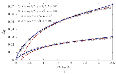
Figure 1: Numerical check of the interpolation formula of Eq. (32) between the non critical and the critical regimes of the FCS of the transverse magnetization $\chi_{\mathfrak{M}_{z}}(\lambda)$. We represent $\Delta_{\rm P}$, defined in Eq. (91), as a function of $x=2L|\log|h||/\gamma$, for different fixed values of $\gamma$ and $L$, and varying $h$. The dots have been calculated numerically using Eq. (17) for $\chi_{\mathfrak{M}_{z}}(\lambda)$. As we explain in Appendix C, $\Delta_{\text{P}}\sim\log\tau_{V}(x)$ for large $L$. The solid curves represent the expansion (34) around $x=0$ up to order $O(x^{4})$ of $\log\tau_{V}(x)$. The dashed curves correspond to the asymptotic behaviour (35) for large $x$ of this $\tau$-function.

It is an interesting question to understand whether the subleading corrections discussed in the previous section (cf. Eqs.  (21),(22)) are also encapsulated in the expansion of the $\tau$-function in Eq. (34).

III.4 The case $\gamma=0$

At $\gamma=0$, the XY spin chain after a Jordan-Wigner transformation reduces to a model of spinless fermions hopping on a one dimensional lattice, that is—up to a constant—

$$H_{XY}|_{\gamma=0}=\frac{1}{2}\sum_{l=1}^{N}(c^{\dagger}_{l}c_{l+1}+H.c.)-h\sum_{l=1}^{N}c^{\dagger}_{l}c_{l}.$$ (36)

By further assuming $0\leq h<1$, let us define $k_{F}\equiv\arccos h$, with $0<k_{F}\leq\pi/2$. The ground state of Eq. (36) is then a Fermi sea, where all the single-particle states with momenta $\phi\in[k_{F},2\pi-k_{F}]$ are filled. The average transverse magnetization per site is $\lim_{N\rightarrow\infty}N^{-1}\langle\mathfrak{M}_{z}\rangle=2\rho-1$, with $\rho=1-\frac{k_{F}}{\pi}$, the average ground state fermion density. In spin language, the model in Eq. (36) is also dubbed the XX chain and corresponds to the zero anisotropy limit of the XXZ spin chain Kbook .

The FCS of the transverse magnetization at $\gamma=0$ can be determined directly, by studying the $\gamma\rightarrow 0$ limit of the symbol in Eq. (18). The resulting function is piecewise constant, with two jump discontinuities at $\phi=\{k_{F},2\pi-k_{F}\}$. An immediate application of Eq. (70) leads to Abanov

$$\log\chi_{\mathfrak{M}_{z}}(\lambda)|_{\gamma=0}=(2\rho-1)\lambda L+\frac{2\lambda^{2}}{\pi^{2}}\log L+O(1),$$ (37)

valid for large $L$. By calculating the Fourier transform of the analytic continuation to imaginary $\lambda$ ($\lambda\to i\lambda$) of the FCS in Eq. (37), one obtains the probability distribution of the transverse magnetization at $\gamma=0$. For $L\gg 1$, this is a Gaussian, with mean centered at $\mu=L(2\rho-1)$ and variance $\sigma^{2}=4\log L/\pi^{2}$. The Shannon entropy of the transverse magnetization at $\gamma=0$ scales then as $O(\log\log L)$. Its sublogarithmic behaviour (cf. Sec.  III.2) is a consequence of the conservation of the total transverse magnetization $\lim_{N\rightarrow\infty}\sum_{l=1}^{N}\sigma_{l}^{z}$: when the interval $A$ is big, large fluctuations of the transverse magnetization are severely suppressed. Furthermore, the limits $\lambda\rightarrow\pm\infty$ and $L\rightarrow\infty$ cannot be interchanged at $\gamma=0$, and STN ; Franchini the EFP of the transverse magnetization is, for $L\gg 1$, $O(e^{-L^{2}})$ contrary to what happens at $\gamma\not=0$ where it decays exponentially, cf. Sec. III.1. The Gaussian decay can also be interpreted as an arctic phenomenon (see e.g. Refs. Stephan ; Allegra ): taking imaginary time, one can argue that, if the transverse magnetization is conserved, the ferromagnetic string generates an area of order $L^{2}$ in which all the degrees of freedom are frozen. The fluctuating degrees of freedom outside the frozen region are described by a massless, but not conformal, field theory.

We will see how these conclusions change for the staggered magnetization in Sec. IV.3 and the domain walls in Sec. V.3.

IV Example II: The staggered transverse magnetization

Another observable whose ground state fluctuations can be fully characterized within our formalism is the transverse staggered magnetization, defined as

$$\mathfrak{M}_{s}=\sum_{l\in A}(-1)^{l+1}\sigma^{z}_{l}.$$ (38)

In this Section we present an exact and comprehensive study of its fluctuations for the XY chain. Our results also apply in the limit $\gamma\rightarrow 0$, which corresponds to the zero anisotropy case of the XXZ spin chain, Sec. IV.3. Partial computations of the staggered magnetization FCS have been done in Groha for this model in the scaling limit, by relying on field theoretical tools.

IV.1 Full Counting Statistics

For the staggered magnetization, cf. Eq. (10), we have $M=2I_{s}$, where ${I_{s}}=\text{diag}(1,-1,1,-1,\dots)$ and $N=0$. The length of the interval $A$ will be taken for convenience $2L$. By applying the results in Sec. II, we end up with the following determinant representation for the ground state FCS

$$\chi_{\mathfrak{M}_{s}}(\lambda)=(-\sinh^{2}\lambda)^{L}\det[G_{s}],$$ (39)

where $G_{s}$ is a block Toeplitz matrix, built from the $2\times 2$ blocks $g_{lm}$ ($l,m=1,\dots,L$), given by

$$g_{lm}=\begin{bmatrix}\coth(\lambda)+(G_{ba})_{2(l-m)}&(G_{ba})_{2(l-m)-1}\\ (G_{ba})_{2(l-m)+1}&-\coth(\lambda)+(G_{ba})_{2(l-m)}\end{bmatrix}.$$ (40)

Generalizing the discussion of Sec. III.1, the symbol of the block Toeplitz matrix $G_{s}$ is the Fourier transform $\tau(\phi)$ of the $2\times 2$ matrix $g_{lm}$, that is

$$\tau(\phi)=\begin{bmatrix}\coth(\lambda)+h_{+}(\phi)&e^{-i\phi/2}h_{-}(\phi)\\ e^{i\phi/2}h_{-}(\phi)&-\coth(\lambda)+h_{+}(\phi)\end{bmatrix},$$ (41)

with $h_{\pm}(\phi)=(e^{i\theta(\phi/2)}\pm e^{i\theta(\phi/2-\pi)})/2$. For $\lambda\in\mathbb{R}$, the matrix elements of $\tau$ have winding number zero and the large-$L$ limit of the FCS can be then computed by recalling a generalization of the Szegő theorem due to H. Widom Widom2 ; Widom3 ; Widom4 and a conjecture formulated in Ares , see again Appendix A.

In particular, for $|h|\not=1$, the matrix elements of $\tau(\phi)$ do not have zeros or jump discontinuities for $\phi\in[0,2\pi]$. The Szegő-Widom theorem Widom2 then applies and one obtains

$$\log\chi_{\mathfrak{M}_{s}}(\lambda)=L\left[\log(-\sinh^{2}\lambda)+\int_{0}^{2\pi}\frac{d\phi}{2\pi}\log(\det\tau(\phi))\right]\\ +O(1).$$ (42)

The $O(1)$ term in Eq. (42) can be also estimated numerically, see Eq. (78).

At the quantum critical point, the matrix elements of the symbol $\tau(\phi)$ have a jump discontinuity at $\phi=0$. We can then apply a generalization of Fisher-Hartwig theorem non-rigorously derived in Ares , see Eqs. (79) and (80), and it turns out

$$\log\chi_{\mathfrak{M}_{s}}(\lambda)=L\left[\log(-\sinh^{2}\lambda)+\int_{0}^{2\pi}\frac{d\phi}{2\pi}\log(\det\tau(\phi))\right]\\ -\beta^{2}_{s}(\lambda)\log(L)+O(1),$$ (43)

where $\beta_{s}(\lambda)=\frac{1}{\pi}\arctan(\tanh^{2}\lambda)$.

Universal terms in the critical FCS.— In the limit $|\lambda|\rightarrow\infty$, the FCS is proportional to the probability of observing an antiferromagnetic domain of length $2L$ in the ground state. More explicitly, from Eq. (7) and Eq. (38), it turns out that

$$\langle e^{\lambda\mathfrak{M}_{S}}\rangle\stackrel{{\scriptstyle\lambda\gg 1}}{{\rightarrow}}e^{2\lambda L}\langle P_{\uparrow\downarrow\dots\uparrow\downarrow}\rangle,$$ (44)

where $P_{\uparrow\downarrow\dots\uparrow\downarrow}$ is the projector onto an antiferromagnetic configuration of transverse spins of length $2L$. The ground state expectation value of such a projector will be denoted by $\mathcal{E}_{s}(h)$.

Therefore, in the limit $|\lambda|\rightarrow\infty$, the prefactor of the logarithmic term in Eq. (43) has a CFT interpretation, since a staggered sequence of spins in the $z$-direction renormalizes to a linear combination of fixed boundary conditions for the longitudinal spins ARV . Consistently one has $\beta_{s}^{2}(\pm\infty)=c/8=1/16$ as for the transverse magnetization, cf. Sec. III.1. At criticality, one expects Stephan also subleading $O(L^{-1}\log L)$ corrections to Eq. (43). By generalizing the method of Ref. Stephan , see Appendix A below Eq. (80), we are able to determine them for $\gamma>0$ and it turns out

$$-\frac{\gamma^{2}+1}{2\pi^{3}\gamma}\frac{\tanh^{2}\lambda}{\tanh^{4}\lambda+1}\arctan^{2}(\tanh^{2}\lambda)L^{-1}\log L.$$ (45)

Details of the derivation of Eq. (45), together with a numerical check, are given in Appendix C. Notice that for $|\lambda|\rightarrow\infty$, Eq. (45) agrees with the CFT prediction given in Eq. (22) provided $\xi_{\text{fixed}}(\gamma)=(\gamma^{2}+1)/(8\gamma)$.

IV.2 The probability distribution at criticality

The probability distribution of the staggered magnetization is defined as in Eq. (24). Being all the eigenvalues of $\mathfrak{M}_{s}$ even integers, the relation $\chi_{\mathfrak{M}_{s}}(i\lambda)=\chi_{\mathfrak{M}_{s}}(i\lambda+\pi)$ still holds and therefore also Eq. (25). We will be then interested in estimating the large-$L$ limit of the Fourier transform

$$\mathcal{P}_{s}(M)=\int_{0}^{\pi}\frac{d\lambda}{2\pi}e^{-iM\lambda}\chi_{\mathfrak{M}_{s}}(i\lambda).$$ (46)

The analytic continuation of the symbol in Eq. (41) to imaginary $\lambda$ introduces a winding when $|h|<1$ for $\lambda\in[\pi/4,3\pi/4]$. At criticality instead, the Wick rotation $\lambda\to i\lambda$ is allowed and the large $L$-limit of Eq. (46) can be obtained in complete analogy to what is done in Sec. III.2, see also Appendix B. One finds

$$\mathcal{P}_{s}(M)=\frac{~{}e^{-\frac{M^{2}}{2\sigma^{2}L}}}{\sqrt{2\pi\sigma^{2}L}}\left[1+B\cos\frac{\pi M}{2}L^{-\frac{1}{4}}\right],$$ (47)

with

$$\sigma^{2}=2-\frac{4(\gamma^{2}+1)^{2}\arccos(2\gamma/(\gamma^{2}+1))}{\pi|\gamma^{4}-1|}.$$ (48)

In this case, $\mu=0$ and $\log B$ is the $O(1)$ term in the expansion (43) of $\log\chi_{\mathfrak{M}_{s}}(i\pi/2)$. Note that $\chi_{\mathfrak{M}_{s}}(i\pi/2)=\det[G_{ba}]$, and the correlation matrix $G_{ba}$ is Toeplitz. Hence, in this particular case, one can use the Fisher-Hartwig conjecture (70) instead of (79), which allows us to determine $B$. In fact, applying (70), we obtain $\chi_{\mathfrak{M}_{s}}(i\pi/2)\sim BL^{-1/4}$, and $B$ is given by Eq. (71). For $\gamma=1$, its expression is specially compact, $B=2^{-1/6}e^{1/4}\mathfrak{A}^{-3}$.

The Gaussian form of the probability distribution implies that the Shannon entropy of the staggered magnetization also scales as $O(\log L)$ for large $L$.

IV.3 The case $\gamma=0$

The fluctuations of the staggered magnetization at $\gamma=0$ are also interesting, since they depend on the value of the transverse field. Let us assume, without loss of generality, $0\leq h<1$ and define, as in Sec. III.4, $k_{F}=\arccos h$; also we will refer to the case $h=0$ as half-filling.

At $\gamma=0$ and away from half-filling, the matrix elements in Eq. (41) are piecewise functions of $\phi$ with two jump discontinuities at $\phi=\{2k_{F},2\pi-2k_{F}\}$. By applying the conjecture in Eq. (79) and in particular Eq. (80), it is possible to calculate the large-$L$ limit for the FCS of the staggered magnetization as follows

$$\log\chi_{\mathfrak{M}_{s}}(\lambda)|_{\gamma=0}=\frac{2k_{F}L}{\pi}\log(\cosh 2\lambda)\\ +\frac{1}{2\pi^{2}}\log^{2}(\cosh 2\lambda)\log L+O(1).$$ (49)

For $h=0$ instead, the matrix elements of the symbol in Eq. (41) when evaluated at $\gamma=0$ are piecewise functions of $\phi$ but with only one jump discontinuity located at $\phi=2k_{F}$. The results in Eqs. (79)-(80) are still valid but the large-$L$ asymptotics is now

$$\log\chi_{\mathfrak{M}_{s}}^{\text{h=0}}(\lambda)|_{\gamma=0}=L\log(\cosh 2\lambda)\\ -2\beta^{2}(\lambda)\log L+O(1),$$ (50)

with $\beta(\lambda)$ defined below Eq. (20).

As we already observed in (44), in the limit $|\lambda|\to\infty$, the FCS is proportional to the probability of finding an antiferromagnetic string in the ground state. There is a qualitative difference between the two limits $|\lambda|\rightarrow\infty$ of Eq. (44) at half-filling and away from it. In the first case, the large-$L$ limit commutes with the large-$\lambda$ limit and the latter can be calculated directly from Eq. (50) with the result

$$\log\mathcal{E}_{s}(h=0)=-L\log 2-\frac{1}{8}\log L+O(1).$$ (51)

At $h=0$, the probability of observing a region with antiferromagnetic order within the ground state of the XX spin chain is exponentially suppressed by its length, i.e. is $O(e^{-L})$. It also contains a logarithmic correction $O(\log L)$ whose prefactor is compatible with the CFT interpretation recalled at the end of Sec. III.1. For $h=\gamma=0$, an antiferromagnetic string of transverse spins renormalizes BS at large distances to a Dirichlet boundary condition for a compactified boson with central charge $c=1$. The prefactor of the subleading logarithmic contribution in Eq. (51) is then $-c/8=-1/8$. It is natural to expect the same logarithmic correction with prefactor $-1/8$ also in the gapless phase Kbook of the XXZ spin chain. To the authors best knowledge, this has not been verified yet.

Away from half-filling, the large-$L$ limit and the large-$\lambda$ limit do not commute any longer. Mathematically, this is due to the fact that the determinant of the symbol in Eq. (41) in the limit $|\lambda|\rightarrow\infty$, and for $\gamma=0,~{}h>0$, vanishes along the interval $I\equiv[2k_{F},2\pi-2k_{F}]$. Then, Eqs. (79) and (80) cannot be used to derive its large-$L$ asymptotics. For scalar symbols which vanish on an interval $I\subset[0,2\pi]$, the asymptotics of the corresponding Toeplitz determinant was worked out by H. Widom in Widom , see Eq. (77). By generalizing such a result, see Eq. (81), we conjecture that

$$\log\mathcal{E}_{s}(h>0)=L^{2}\log\sin k_{F}-L\log 2\\ -\frac{1}{4}\log L+O(1).$$ (52)

In Fig. 2, we check numerically the above conjecture. The points are the values for $\log\mathcal{E}_{s}(h>0)$ obtained from the numerical computation of Eq. (39) at $\gamma=0$ and $h>0$ while the curves correspond to the analytical prediction in Eq. (52).

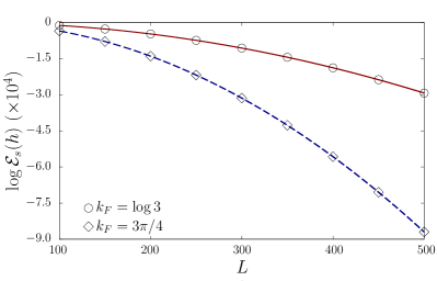
Figure 2: Numerical check of the expansion conjectured in Eq. (52) for the formation probability of an antiferromagnetic domain in a XX spin chain with Fermi momentum $k_{F}\neq\pi/2$. The dots have been obtained by calculating numerically the determinant in Eq. (39) in the limit $\lambda\to-\infty$. The curves correspond to the conjectured expansion (52); the $O(1)$ term has been determined from $\log\mathcal{E}_{s}(L=500)-500^{2}\log\sin k_{F}-500\log 2-1/4\log(500)$, taking as $\mathcal{E}_{s}(L=500)$ the value obtained numerically for this quantity at $L=500$ for each Fermi momentum considered.

The physical explanation of Eq. (52) mimics the discussion in Sec. III.4. For $h>0$, the conservation law $[H_{XY}|_{\gamma=0},\mathfrak{M}_{z}]=0$ requires all the eigenstates of the XX Hamiltonian to be eigenstates of $N^{-1}\mathfrak{M}_{z}$ with eigenvalue different from zero in the thermodynamic limit $N\rightarrow\infty$. Therefore the probability of observing a large region with antiferromagnetic order at zero temperature must fall off more quickly, as $O(e^{-L^{2}})$, than at $h=0$. At half-filling, instead, the Néel state $|\uparrow\downarrow\dots\uparrow\downarrow\rangle$ is not orthogonal to the ground state and its overlap ARV decays exponentially as $O(e^{-N})$, leading to an exponential decay of $\mathcal{E}_{s}(h=0)$ in Eq. (51).

Finally, we note that at criticality Eqs. (49) and (50) imply that the probability distribution of the staggered magnetization is Gaussian at $\gamma=0$, with variance of $O(L)$. Therefore its Shannon entropy is $O(\log L)$ for large $L$. There are also subleading power law corrections of the type $L^{-\alpha}$ as in Eq. (47) but with exponent $\alpha=1/2$.

V Example III: The domain walls

We characterize exactly at large $L$ the fluctuations of the number of domain walls in the XY spin chain, that is

$$\mathfrak{K}=\sum_{l\in A}(1-\sigma_{l}^{x}\sigma_{l+1}^{x}).$$ (53)

At $\gamma=1$, this observable can be accessed by a Kramers-Wannier transformation applied to the transverse magnetization Demler . Our analysis will be more general and valid for any values of the anisotropy $\gamma>0$. Eventually, we will also show how our results for the FCS allow determining analytically the EFP of the longitudinal magnetization $\mathfrak{M}_{x}=\sum_{l\in A}\sigma_{l}^{x}$. The latter has been recently discussed in Collura resorting to certain numerical approximations.

V.1 The Full Counting Statistics

By applying the Jordan-Wigner transformation in Eq. (13), the operator $\mathfrak{K}$ of Eq. (53) can be put in the form of Eq. (6) with

$$(M)_{lm}=\delta_{|l-m|,1},~{}(N)_{lm}=\delta_{|l-m|,1}\mathop{\mathrm{sign}}\nolimits(m-l),$$ (54)

for $l,m=1,\dots,L+1$. Even if the matrix $N$ in Eq. (54) is non-zero, it is simple enough to carry over the calculation of the matrix exponential in Eq. (11). One finds, see Appendix C, the following determinant representation for the domain wall FCS

$$\chi_{\mathfrak{K}}(\lambda)=\det[G_{\mathfrak{K}}].$$ (55)

The $L\times L$ matrix $G_{\mathfrak{K}}$ is of Toeplitz type with symbol, cf. Eq. (18),

$$g_{\mathfrak{K}}(\phi)=\frac{e^{2\lambda}+1}{2}+\frac{e^{2\lambda}-1}{2}e^{-i\phi}e^{i\theta(\phi)}.$$ (56)

The analysis of its large-$L$ behaviour is then straightforward. Indeed the same Eqs. (19) and (20) hold for the large-$L$ limit of the domain wall FCS upon the replacement of the symbols: $g_{\mathfrak{M}_{z}}(\phi)\to g_{\mathfrak{K}}(\phi)$.

EFP of the order parameter.—The exact expression derived in Eq. (55) for the domain wall FCS is in accordance with the Kramers-Wannier duality between longitudinal and transverse spin configurations analyzed in ARV for the Ising spin chain. In particular, by comparing Eq. (56) with Eq. (18) at $\gamma=1$ and taking for simplicity $h>0$, one concludes that

$$\chi_{\mathfrak{K}}(\lambda)|_{h}=e^{\lambda L}\chi_{\mathfrak{M}_{z}}(-\lambda)|_{1/h},~{}~{}~{}h>0.$$ (57)

In the limit $\lambda\rightarrow-\infty$, Eq. (57) implies

$$\lim_{\lambda\rightarrow-\infty}\chi_{\mathfrak{K}}(\lambda)=\langle P_{\rightarrow\dots\rightarrow}+P_{\leftarrow\dots\leftarrow}\rangle,$$ (58)

where $P_{\rightarrow\dots\rightarrow}$ and $P_{\leftarrow\dots\leftarrow}$ are projectors onto states that contain a ferromagnetic region of length $L$ with spins aligned along the $x$-axis. The Kramers-Wannier duality maps both these configurations to one where all the spins are polarized along the positive $z$-axis ARV . Notice that such a conclusion follows directly from Eq. (57). Analogously, an antiferromagnetic domain of longitudinal spins is the Kramers-Wannier dual of a ferromagnetic domain of negatively polarized transverse spins ARV . This last statement is implied by the limit $\lambda\rightarrow\infty$ of Eq. (57).

In absence of a longitudinal field coupling to $\sigma_{l}^{x}$, the two projectors in Eq. (58) have the same ground state expectation value. The latter is the EFP, $\mathcal{E}_{x}(h)$, of the order parameter $\mathfrak{M}_{x}|_{A}=\sum_{l\in A}\sigma_{l}^{x}$ restricted to the subsystem $A$. For the Ising spin chain, and positive transverse field, after some contour integral manipulations outlined in Appendix C, we obtain the compact expressions for $\mathcal{E}_{x}(h)$

$$\log\mathcal{E}_{x}(h)=\begin{cases}L\bigl{[}\int_{0}^{1/h}\frac{dy}{\pi}~{}K(y^{2})-\log 2\bigr{]}+O(1),~{}~{}~{}h>1\\ L\left(\frac{2\mathfrak{C}}{\pi}-\log 2\right)-\frac{1}{16}\log L+O(1),~{}~{}~{}h=1\\ -L\int_{0}^{h}\frac{dy}{\pi}\frac{1}{y}\left(K(y^{2})-\frac{\pi}{2}\right)+O(1),~{}~{}~{}h<1.\end{cases}$$ (59)

The function $K(y)$ is the complete elliptic integral of the first kind, written in Mathematica notations, while $\mathfrak{C}=\frac{1}{2}\int_{0}^{1}dy~{}K(y^{2})$ is the Catalan constant. The first few terms of the series expansion about $h=0$ of Eq. (59) reproduce the approximate formula proposed recently in Collura . Of course the calculation of the EFP for the order parameter could be extended to any $\gamma>0$, simply by considering the limit $\lambda\rightarrow-\infty$ of the symbol in Eq. (56). Though the extension of Eq. (59) to $\gamma\not=1$ has not a nice compact form.

Universal terms in the critical FCS.— As expected from the discussion at the end of Sec. III.1, the prefactor of the $O(\log L)$ term of the critical domain wall FCS in the limit $\lambda\rightarrow\pm\infty$ is $\gamma$-independent and with value: $-\frac{1}{16}$. By pushing the asymptotics analysis of the Toeplitz determinant in Eq. (55) further, one can single out along the critical lines also an $O(\log L/L)$ term, see Eq. (73),

$$-\frac{2\gamma-1}{2\pi^{3}\gamma}\tanh(2\lambda)\arctan^{2}(\tanh\lambda)L^{-1}\log L,$$ (60)

whose presence can be checked numerically, see Fig. 3 and Appendix C.

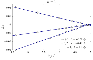
Figure 3: Numerical check of the $O(L^{-1}\log L)$ term in the expansion of $\log\chi_{\mathfrak{K}}(\lambda)$ along the critical line $h=1$. We plot $\Delta_{\mathfrak{K}}$, defined in Eq. (96), as a function of $\log L$ for several fixed values of $\gamma$ and $\lambda$, and choosing $L_{0}=10^{3}$. The dots have been obtained by calculating numerically $\chi_{\mathfrak{K}}(\lambda)$ through Eq. (55). The lines represent $d_{\mathfrak{K}}\log(L/L_{0})$, taking for $d_{\mathfrak{K}}$ the coefficient of the $O(L^{-1}\log L)$ term predicted in Eq. (60).

Notice however that the lattice result in Eq. (60) has not a definite sign as a function of $\gamma>0$; it vanishes for $\gamma=1/2$. These considerations suggest that the limit $\lambda\rightarrow\pm\infty$ of Eq. (60) has not an immediate CFT interpretation Stephan and deserves futher study.

Painlevé V equation in the scaling limit.— An interesting consequence of Eq. (56) is that the same analysis of the scaling limit discussed in Sec. III.3 for the transverse magnetization also applies to the domain walls. In the limits $|h|\rightarrow 1$, $L\rightarrow\infty$ keeping $x=2L|\log|h||/\gamma$ finite, the domain wall FCS interpolates from the critical ($x\ll 1$) asymptotics given in Eq. (70) to the off-critical asymptotics ($x\gg 1$) in Eq. (68). The crossover is again analytically captured by Eq. (32) after replacing $g_{\mathfrak{M}_{z}}(\phi)$ with $g_{\mathfrak{K}}(\phi)$. In particular, since the Fisher-Hartwig exponent $\beta(\lambda)$ in Eq. (32) is the same for the transverse magnetization and the domain walls, the expansion of the Painlevé V $\tau$-function in Eq. (34) is also identical. A numerical check of the interpolation formula in Eq. (32) adapted to the domain wall fluctuations is given in Fig. 4.

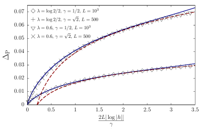
Figure 4: Numerical analysis of the crossover between the non-critical and the critical behaviour of the FCS of the number of domain walls, $\chi_{\mathfrak{K}}(\lambda)$. We study the quantity $\Delta_{\rm P}$, defined in Eq. (91) but replacing $\chi_{\mathfrak{M}_{z}}$ and $g_{\mathfrak{M}_{z}}$ by $\chi_{\mathfrak{K}}$, $g_{\mathfrak{K}}$, versus the ratio $x=2L|\log|h||/\gamma$; we vary $h$, keeping $\gamma$, $\lambda$ and $L$ fixed. The dots correspond to calculate numerically $\chi_{\mathfrak{K}}(\lambda)$ using Eq. (55). As we point out in Appendix C, we expect $\Delta_{\text{P}}\sim\log\tau_{V}(x)$ when $L$ is large enough. The solid curves represent the expansion (34) of the logarithm of the Painlevé V $\tau$-function around $x=0$ up to order $O(x^{4})$. The dashed curves are the asymptotic behaviour (35) of this function for $x\to\infty$.

V.2 The probability distribution at criticality

The eigenvalues of the operator $\mathfrak{K}$ in Eq. (53) are the even integers $2n_{w}$ where $n_{w}=0,\dots,L$ is the number of domain walls present in the subsystem $A$. Therefore, the probability distribution $P_{\mathfrak{K}}(W)=\langle\delta(\mathfrak{K}-W)\rangle$ can be recast in the form of Eq. (25) and we will calculate here

$$\mathcal{P}_{K}(W)=\int_{0}^{\pi}\frac{d\lambda}{2\pi}e^{-iW\lambda}\chi_{\mathfrak{K}}(i\lambda),$$ (61)

at the quantum critical point $|h|=1$. The exponential decay for large $L$ of the domain wall FCS already implies that $\mathcal{P}_{K}(W)$ is a Gaussian, as pointed out in Sec. III.2. More formally, by applying the saddle point analysis of Appendix B one finds

$$\mathcal{P}_{K}(W)=\frac{~{}e^{-\frac{(W-\mu L)^{2}}{2\sigma^{2}L}}}{\sqrt{2\pi\sigma^{2}L}}\left[1+B\cos\frac{\pi W}{2}L^{-\frac{1}{4}}\right],$$ (62)

with parameters $\mu,\sigma$ given by

$$\mu=1-\frac{2\gamma}{\pi(\gamma+1)}\left(1+\frac{\text{arccosh}(\gamma)}{\sqrt{\gamma^{2}-1}}\right),$$ (63)

and

$$\sigma^{2}=\frac{\gamma^{2}(\gamma-1)+7\gamma+1}{(\gamma+1)^{3}}.$$ (64)

The coefficient $\log B$ is the $O(1)$ term in the expansion of $\log\chi_{\mathfrak{K}}(\lambda)$ at $\lambda=i\pi/2$. Therefore, it can be calculated from Eq. (71). We omit to write here the explicit form of $B$ since it is a lengthy expression. In Fig. 5, we check numerically the probability distribution in Eq. (62).

At the critical point $|h|=1$, $\gamma\not=0$. the Shannon entropy of the domain wall probability distribution scales as $O(\log L)$ for large $L$. In fact, the same conclusion also applies to the other critical point of the XY chain: $\gamma=0$ and $|h|<1$. This will be discussed in detail in the next Section.

In the non-critical regions, $|h|\neq 1$, $\gamma>0$, $\mathcal{P}_{K}(W)$ is also a Gaussian for large $L$, but there is no a $L^{-1/4}$ subleading correction, see Eqs. (85) and (86) of Appendix B. In that Appendix, we give the technical details to obtain those results.

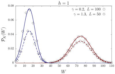
Figure 5: Probability distribution $\mathcal{P}_{K}(W)$ of domain walls in an interval of length $L$ along the critical line $h=1$. The dots correspond to the direct numerical integration of Eq. (61), considering for $\chi_{\mathfrak{K}}(\lambda)$ the asymptotic expansion obtained by applying the Fisher-Hartwig conjecture. The solid and dashed curves represent the analytical approximation found in Eq. (62) for $W=4n$ and $W=4n+2$ respectively, with $n\in\mathbb{N}$. For the case $\gamma=0.2$ and $L=100$, $B=0.327387$ while, for $\gamma=1.3$ and $L=50$, $B=0.682844$.

V.3 The case $\gamma=0$

We investigate the FCS of the domain walls for the XX spin chain, cf. Eq. (36). For simplicity, we assume $0\leq h<1$ and define $k_{F}=\arccos h$ as in Sec. III.4. In the limit $\gamma\rightarrow 0$, the symbol in Eq. (56) is a piecewise function of $\phi$ with two jump discontinuities at $\phi=\{k_{F},2\pi-k_{F}\}$. We can then apply Eq. (70) and obtain the following large-$L$ asymptotics of the Toeplitz determinant in Eq. (55)

$$\log\chi_{\mathfrak{K}}(\lambda)|_{\gamma=0}=a(\lambda)L\\ +\frac{2}{\pi^{2}}\Re\left[\text{arctanh}^{2}\bigl{(}\tanh\lambda e^{-ik_{F}}\bigr{)}\right]\log L\\ +O(1).$$ (65)

Eq. (65) shows that the domain wall FCS decays exponentially with the subsystem length $L$. The coefficient $a(\lambda)$ and the $O(1)$ term in Eq. (65) can be explicitly determined but their expressions are rather lengthy. For $|h|<1$, the logarithm of the FCS also contains an $O(\log L/L)$ subleading contribution that can be calculated from Eq. (73) with the result

$$\frac{4}{\pi^{3}}\Re\left[\frac{ie^{ik_{F}}\tanh\lambda}{e^{2ik_{F}}-\tanh^{2}\lambda}\text{arctanh}^{2}\left(e^{-ik_{F}}\tanh\lambda\right)\right]\\ \times L^{-1}\log L.$$ (66)

Contrary to the case of the transverse magnetization discussed in Sec. III.4, Eqs. (65) and (66) are finite in the limits $\lambda\rightarrow\pm\infty$. They can then be used to test the universality and semi-universality of the prefactors of the $O(\log L)$ and $O(\log L/L)$ terms.

In particular for $\lambda\rightarrow-\infty$, the FCS in Eq. (65) is proportional to the formation probability of a ferromagnetic domain of longitudinal spins. This spin configuration flows toward a Neumann boundary condition for a free boson compactified on a circle SMA . In this case, as also pointed out in Sec. IV.3, CFT Stephan predicts that the prefactor of the $O(\log L)$ term is $-1/8$. It is easy to realize that the exact lattice result in Eq. (65) agrees with the field theory conjecture only at half-filling. A similar discrepancy for $k_{F}\not=\pi/2$ was also pointed out in other comparisons between CFT expectations and lattice calculations for free fermions, see for instance ZA ; SD . At half-filling, the limit $\lambda\rightarrow-\infty$ in Eq. (66) is also consistent with Eq. (21) at $c=1$ if the non-universal extrapolation length is $\xi=1$.

In the limit $\lambda\rightarrow\infty$, the domain wall FCS is proportional to the formation probability of an antiferromagnetic domain of longitudinal spins. To the authors best knowledge, it is not clear to which conformal boundary condition of a free bosonic theory this spin configuration should flow. Anyway, the limit $\lambda\rightarrow\infty$ of the prefactor in the $O(\log L)$ in Eq. (65) still admits a $c=1$ CFT interpretation while Eq. (66) is in agreement with Eq. (22), provided one postulates the presence of a boundary condition changing operator Cardy  with conformal dimension $h_{\text{bcc}}=1/8$.

We close this Section by highlighting an exact expression for the probability of formation of a ferromagnetic length-$L$ domain of longitudinal spins at half-filling and zero temperature. By evaluating the limit $\lambda\rightarrow-\infty$ and $k_{F}\rightarrow\pi/2$ in Eqs. (65)-(66), including the $O(1)$ term in Eq. (71) we obtain

$$\log\mathcal{E}_{x}(h=0)|_{\gamma=0}=\left(\frac{2\mathfrak{G}}{\pi}-\log 2\right)L-\frac{1}{8}\log L+\\ \frac{\mathfrak{G}}{\pi}-\frac{9\log 2}{8}+2\log[G(3/4)G(5/4)]-\frac{7\zeta(3)}{8\pi^{2}}+\\ \frac{1}{8\pi}L^{-1}\log L+O(L^{-1})$$ (67)

where $\zeta(z)$ is the Riemann zeta. We quote the result in Eq. (67) as a mathematical curiosity: the appearance of the Riemann zeta function with odd argument in calculations of formation probabilities in the XXZ spin chain is the leitmotif of Ref. BK .

VI Conclusions

In this paper, we characterized exactly the quantum fluctuations of the transverse, staggered magnetization and the domain walls in the ground state of the XY spin chain.

We also derived an analytic expression that captures the behavior of the full counting statistics for the transverse magnetization and the domain walls in the scaling limit, close to the quantum phase transition. The interpolation formula is built from the solution of a Painlevé V equation, for which it is possible to write down an explicit power series expansion.

The lattice calculations allow a direct verification of the field theoretical conjectures formulated in Stephan for the $O(\log L)$ and $O(\log L/L)$ subleading contributions to the critical formation probabilities. These are extracted as limits for a large value of the coupling $\lambda$ of the cumulant generating functions. In particular, we showed that the field theory predictions for the semi-universal $O(\log L/L)$ term do not have an obvious application to the domain walls when $\gamma<1/2$. An analogous issue, already observed in ZA ; SD , is found for their critical fluctuations in the XX spin chain away from half-filling.

By determining exactly the domain wall full counting statistics, we have also calculated the probability of observing in the ground state a ferromagnetic and antiferromagnetic domain of transverse and longitudinal spins. Fluctuations of the latter are harder to access since the order parameter is not a quadratic fermionic form.

Our results hinge on the asymptotic expansion of Toeplitz determinants, for which we have also formulated and checked numerically a new conjecture in Appendix A, in particular Eq. (81). The technique is suitable to detect any pattern of order NRV in the transverse direction, by properly modifying the observable $\mathfrak{O}$.

Appendix A Asymptotics of determinants of block Toeplitz matrices

In this paper we made extensive application of several results on determinants of block Toeplitz matrices. We summarize them in this Appendix.

Let $\mathcal{G}$ be an arbitrary matrix valued function of dimension $d\times d$ defined on the unit circle $S^{1}$ and with entries in $L^{1}(S^{1})$. The block Toeplitz matrix $T_{L}[\mathcal{G}]$ with symbol $\mathcal{G}$ is the $L\cdot d$ dimensional matrix built from the Fourier coefficients of the entries of $\mathcal{G}$ such that

$$(T_{L}[\mathcal{G}])_{nm}=(\mathcal{G})_{n-m}=\int_{0}^{2\pi}\frac{d\phi}{2\pi}\mathcal{G}(\phi)e^{i\phi(n-m)}$$

for $n,m=1,\dots,L$. We shall denote by $D_{L}[\mathcal{G}]$ the determinant of $T_{L}[\mathcal{G}]$, i. e. $D_{L}[\mathcal{G}]=\det(T_{L}[\mathcal{G}])$.

First, let us consider the case $d=1$, in which the symbol $g$ is a scalar function and, therefore, $T_{L}[g]$ is a Toeplitz matrix. This is the case of interest in Secs. III and V, where we have expressed the FCS of the magnetization and of domain walls respectively as Toeplitz determinants.

Szegő theorem.—If the symbol $g(\phi)$ is a smooth enough, non vanishing, complex function with zero winding number (i.e. the argument of $g(\phi)$ is continuous and periodic for $\phi\in[0,2\pi]$), then the (Strong) Szegő theorem Szego ; Ibraginov states that

$$\log D_{L}[g]=(\log g)_{0}L+\sum_{k=1}^{\infty}k(\log g)_{k}(\log g)_{-k}+o(1).$$ (68)

Here the $o(1)$ terms decay exponentially with $L$.

Fisher-Hartwig formula.—When the symbol $g(\phi)$ presents zeros or jump discontinuities, the Szegő theorem is not valid anymore. In this case, the Fisher-Hartwig formula Fisher ; Basor gives the asymptotic behavior of the determinant. Suppose that the symbol has $R$ zeros and/or discontinuities at the points $0\leq\phi_{1},\dots,\phi_{R}<2\pi$, and we can factorize $g(\phi)$ in the form

$$g(\phi)=V(\phi)\prod_{r=1}^{R}(2-2\cos(\phi-\phi_{r}))^{\alpha_{r}}e^{i\beta_{r}(\phi-\phi_{r}-\pi{\rm sign}(\phi-\phi_{r}))},$$ (69)

where $V(\phi)$ is a function satisfying the conditions of the Szegő theorem, and $\Re\alpha_{r}>-1/2$, $\beta_{r}\in\mathbb{C}$ with $\alpha_{r}\pm\beta_{r}\neq-1,-2,\dots$ for all $r$. Then, according to the Fisher-Hartwig formula,

$$\log D_{L}[g]=(\log V)_{0}L+\sum_{r=1}^{R}(\alpha_{r}^{2}-\beta_{r}^{2})\log L\\ +E(V,\{\alpha_{r}\},\{\beta_{r}\},\{\phi_{r}\})+o(1)$$ (70)

where

$$E(V,\{\alpha_{r}\},\{\beta_{r}\},\{\phi_{r}\})=\sum_{k=1}^{\infty}k(\log V)_{k}(\log V)_{-k}\\ +\sum_{r=1}^{R}[(-\alpha_{r}+\beta_{r})V_{-}(\phi_{r})-(\alpha_{r}+\beta_{r})V_{+}(\phi_{r})]\\ -\sum_{1\leq r\neq r^{\prime}\leq R}(\alpha_{r}-\beta_{r})(\alpha_{r^{\prime}}+\beta_{r^{\prime}})\log\left(1-e^{i(\phi_{r}-\phi_{r^{\prime}})}\right)\\ +\sum_{r=1}^{R}\log\frac{G(1+\alpha_{r}+\beta_{r})G(1+\alpha_{r}-\beta_{r})}{G(1+2\alpha_{r})},$$ (71)

and

$$V_{\pm}(\phi)=\sum_{k=1}^{\infty}(\log V)_{\pm k}e^{\mp i\phi k}.$$ (72)

If the function $V(\phi)$ is smooth enough, then it is conjectured Kozlowski that the $o(1)$ term in (70) can be expressed as a power series in $L^{-1}$. However, here we have numerically found that in some cases the leading $o(1)$ term is of order $O(L^{-1}\log L)$. Following Ref. Stephan , we trace back the origin of these terms to the presence of cusps in the function $V(\phi)$ at the Fisher-Hartwig singularities $\phi_{r}$.

Subleading contributions $O(L^{-1}\log L)$.—In order to determine the contribution $L^{-1}\log L$ to $\log D_{L}[g]$, let us take a symbol that can be factorized in the form (70) such that

$$g(\phi)=V(\phi)e^{i\beta(\phi-\phi_{c}-\pi{\rm sign}(\phi-\phi_{c}))}.$$

That is, it has a jump discontinuity at $\phi=\phi_{c}$. Now we further suppose that $V(\phi)$ has a cusp at $\phi=\phi_{c}$, i. e.

$$V(\phi)\sim\kappa\,(1+\mu^{\pm}(\phi-\phi_{c})),\quad\phi\to\phi_{c}^{\pm},$$

where $\kappa$ is a constant independent of $\phi$ and $\mu^{+}\neq\mu^{-}$. Generalizing the analysis performed in Stephan to this case, we factorize $V(\phi)$ in the form

$$V(\phi)=U(\phi)(1+z)^{\nu(z)}(1+1/z)^{\tilde{\nu}(z)},\,\,z\equiv e^{i(\phi-\phi_{c}-\pi{\rm sign}(\phi-\phi_{c}))},$$

with

$$\nu(z)=\sum_{p=1}^{\infty}\eta_{p}(z+1)^{p},\quad\tilde{\nu}(z)=\sum_{p=1}^{\infty}\eta_{p}(1/z+1)^{p}.$$

The coefficients $\eta_{p}$ must be chosen to smoothen $V(\phi)$ such that $U(\phi)$ be analytic at $\phi_{c}$. Then, in light of Stephan , we conjecture that

$$\log D_{L}[g]=aL+b\log L+c-2\eta_{1}\beta^{2}L^{-1}\log L,$$ (73)

where the coefficients $a$, $b$ and $c$ can be computed using the Fisher-Hartwig conjecture (70). The coefficient $\eta_{1}$ can be determined by taking into account that the function $U(\phi)$ is of class $C^{1}$ at $\phi=\phi_{c}$ iff

$$\lim_{\phi\to\phi_{c}^{-}}U^{\prime}(\phi)=\lim_{\phi\to\phi_{c}^{+}}U^{\prime}(\phi).$$

From this condition it follows that

$$\eta_{1}=\frac{\mu^{-}-\mu^{+}}{2\pi}.$$

In some cases, we have to deal with symbols with two jump discontinuities where the function $V(\phi)$ presents cusps. In this case, we perform the above analysis for each cusp separately and, at the end, the coefficient of the $O(L^{-1}\log L)$ term is the sum of the contribution of the two cusps as we have numerically checked.

Multiple factorizations and non-zero winding.—The symbol $g(\phi)$ may admit more than one factorization (69),

$$g(\phi)=V^{(j)}(\phi)\prod_{r=1}^{R}(2-2\cos(\phi-\phi_{r}))^{\alpha_{r}^{(j)}}e^{i\beta_{r}^{(j)}(\phi-\phi_{r}-\pi\mathop{\mathrm{sign}}\nolimits(\phi-\phi_{r}))}$$

where $j$ is the label of each factorization. In this case, there is a generalization of the Fisher-Hartwig conjecture, proposed in Basor2 and proved in Deift . It can be stated as follows: for $L\to\infty$,

$$D_{L}[g]\sim\sum_{j\in S}e^{(\log V^{(j)})_{0}L}L^{\Omega(j)}e^{E(V^{(j)},\{\alpha_{r}^{(j)}\},\{\beta_{r}^{(j)}\},\{\phi_{r}\})},$$ (74)

where

$$\Omega(j)=\sum_{r=1}^{R}[(\alpha_{r}^{(j)})^{2}-(\beta_{r}^{(j)})^{2}],$$

and

$$S=\{j\,|\,\Re\Omega(j)=\Omega\},\quad\mbox{with}\quad\Omega=\max_{j}\Re\Omega(j).$$

In some situations, the analyzed symbol has winding number $\pm 1$, i.e. it can be written as $g(\phi)=e^{\pm i\phi}V(\phi)$ where the function $V(\phi)$ satisfies the hypothesis of the Szegő theorem. This is the case, for instance, of the symbol of the FCS of domain walls $\chi_{\mathfrak{K}}(i\lambda)$, which has winding number when $|h|>1$ and $\lambda\in[\pi/4,3\pi/4]$. When this occurs, we must resort to another extension of Szegő theorem Fisher ; Hartwig . If $g(\phi)$ has winding number $+1$, the corresponding determinant behaves for large dimension as

$$D_{L}[g]\sim(-1)^{L}m_{L}D_{L+1}[V].$$ (75)

The asymptotics of the determinant $D_{L+1}[V]$ is given by (68) and $m_{L}$ is the $L$-Fourier coefficient of the function

$$m(\phi)=e^{V_{-}(\phi)-V_{+}(\phi)},$$

with $V_{\pm}(\phi)$ as defined in (72). Analogously, if $g(\phi)$ has winding number $-1$, then we have

$$D_{L}[g]\sim(-1)^{L}l_{L}D_{L+1}[V],$$ (76)

where now $l_{L}$ is the $L$-Fourier coefficient of

$$l(\phi)=e^{V_{+}(-\phi)-V_{-}(-\phi)}.$$

In order to estimate the leading contribution of $l_{L}$ and $m_{L}$ for large $L$, it is convenient to analytically continue the functions $l(\phi)$ and $m(\phi)$ from the unit circle to the whole Riemann sphere. Let us call $\mathfrak{V}(z)$, $\mathfrak{l}(z)$ and $\mathfrak{m}(z)$ the analytical continuations of $V(\phi)$, $l(\phi)$ and $m(\phi)$, such that $\mathfrak{V}(e^{i\phi})=V(\phi)$, $\mathfrak{l}(e^{i\phi})=l(\phi)$ and $\mathfrak{m}(e^{i\phi})=m(\phi)$. If we now introduce the Wiener-Hopf factorization for $\mathfrak{V}(z)$,

$$\mathfrak{V}(z)=b_{+}(z)e^{(\log V)_{0}}b_{-}(z),\quad b_{\pm}(z)=e^{\sum_{k>0}(\log V)_{\mp k}z^{\pm k}},$$

then

$$\mathfrak{l}(z)=\frac{b_{-}(1/z)}{b_{+}(1/z)},\quad\mathfrak{m}(z)=\frac{b_{+}(z)}{b_{-}(z)},$$

and $l_{L}$, $m_{L}$ can be expressed as the contour integrals

$$l_{L}=\oint_{|z|=1}\frac{dz}{2\pi i}\frac{b_{-}(z)}{b_{+}(z)}z^{-(L+1)},$$

$$m_{L}=\oint_{|z|=1}\frac{dz}{2\pi i}\frac{b_{+}(1/z)}{b_{-}(1/z)}z^{-(L+1)}.$$

Note that $b_{+}(z)$ is analytic inside the unit circle while $b_{-}(z)$ is analytic outside it. The idea now is to deform the contour of integration from the unit circle to the point at infinity where the term $z^{-L-1}$ cancels the integrand. In general, the integrand presents singularities such as branch points and/or poles outside the unit circle which must be surrounded by the deformed contour. Therefore, the dominant contribution to $l_{L}$ and $m_{L}$ will come from the singularity outside the unit circle closest to it. If this singularity is a pole, we can compute its contribution with the residue theorem. If it is a branch point, we take the branch cuts such that each one connects a branch point outside the unit circle to infinity without intersecting the rest as well as the unit circle. Then, once the contour has been deformed to infinity and runs around the branch cuts, we can apply the Watson lemma for loop integrals, see e.g. Temme ; Jones , to obtain the leading contribution.

Widom theorem.—Another situation of our interest is when the symbol $g(\phi)$ is periodic and supported on a closed interval $I=[0,\omega]\cup[2\pi-\omega,2\pi]$ such that, when it is restricted to this arc, $g(\phi)$ is smooth enough and positive. In this case, Widom Widom showed that

$$\log D_{L}[g]\sim L^{2}\log\sin\frac{\omega}{2}+\\ L\int_{0}^{2\pi}\frac{d\phi}{2\pi}\log g\left(2\arcsin\left(\sin\frac{\omega}{2}\sin\phi\right)\right)-\frac{1}{4}\log L.$$ (77)

Szegő-Widom theorem.—We move now on to the case $d>1$. Genuine block Toeplitz determinants with $d=2$ appear when we study the FCS of the staggered magnetization in Sec. 38. As we will see, we can formulate analogous results to the Szegő theorem and the Fisher-Harwig conjecture as well as the Widom theorem.

Consider a $d\times d$ symbol $\mathcal{G}$. If the entries of $\mathcal{G}(\phi)$ are smooth enough, complex functions and $\det\mathcal{G}(\phi)\neq 0$ with zero winding number, then the Szegő-Widom theorem Widom2 ; Widom3 ; Widom4 gives the asymptotic behaviour of $D_{L}[\mathcal{G}]$,

$$\log D_{L}[\mathcal{G}]=(\log\det\mathcal{G})_{0}L+E[\mathcal{G}]+o(1).$$

The term $E[\mathcal{G}]$ can be written as

$$E[\mathcal{G}]=\log\det T[\mathcal{G}]T[\mathcal{G}^{-1}],$$ (78)

where $T[\mathcal{G}]$, $T[\mathcal{G}^{-1}]$ are the semi-infinite matrices obtained respectively from $T_{L}[\mathcal{G}]$ and $T_{L}[\mathcal{G}^{-1}]$ in the limit $L\to\infty$. The Szegő-Widom theorem reduces to the Szegő theorem for $d=1$.

Conjecture 1.—If the entries of $\mathcal{G}(\phi)$ present jump discontinuities at the points $\phi_{1},\dots,\phi_{R}$, and $\det\mathcal{G}(\phi)$ can be factorized in the Fisher-Hartwig form (69), then $D_{L}[\mathcal{G}]$ behaves as Ares

$$\log D_{L}[\mathcal{G}]=(\log\det\mathcal{G})_{0}L+b\log L+O(1),$$ (79)

where

$$b=\frac{1}{4\pi^{2}}\sum_{r=1}^{R}\mathop{\mbox{Tr}}\nolimits\left[\log(\mathcal{G}_{r}^{-}(\mathcal{G}_{r}^{+})^{-1})\right]^{2},$$ (80)

with $\mathcal{G}_{r}^{\pm}$ the lateral limits of $\mathcal{G}(\phi)$ at the point $\phi_{r}$,

$$\mathcal{G}_{r}^{\pm}=\lim_{\phi\to\phi_{r}^{\pm}}\mathcal{G}(\phi).$$

Note that this result is a generalisation for matricial symbols of that in (70) for non vanishing, scalar symbols with jump discontinuities.

We have also numerically found that in the expansion of $\log D_{L}[\mathcal{G}]$, with jump discontinuities in $\mathcal{G}(\phi)$, may appear terms of order $O(L^{-1}\log L)$. Inspired by the analysis performed for these corrections in the scalar case, we claim that, when $d>1$, they can be related to the presence of cusps in $\det\mathcal{G}(\phi)$ at the discontinuity points $\phi_{r}$. Then, one may repeat the analysis performed for the result conjectured in Eq. (73), but replacing $V(\phi)$ by $\det\mathcal{G}(\phi)$ and $-\beta^{2}$ by the coefficient $b$ given in (80).

Conjecture 2.— Finally, we have also studied symbols $\mathcal{G}(\phi)$ for which $\det\mathcal{G}(\phi)$ is supported on the arc $I$, and therefore the previous results cannot be applied. In analogy to the Widom theorem (77), we conjecture that

$$\log D_{L}[\mathcal{G}]\sim L^{2}\log\sin\frac{\omega}{2}+\\ L\int_{0}^{2\pi}\frac{d\phi}{2\pi}\log\det\mathcal{G}\left(2\arcsin\left(\sin\frac{\omega}{2}\sin\phi\right)\right)\\ -\frac{1}{4}\log L,$$ (81)

if the restriction of $\mathcal{G}(\phi)$ to the interval $I$ satisfies the conditions of the Widom-Szegő theorem.

Appendix B Estimation of the critical Probability Distributions

In this Appendix, we describe the way to obtain the behaviour for large $L$ of the probabilities $\mathcal{P}_{\alpha}(M)$ along the critical lines $h=\pm 1$, $\gamma>0$. The discussion is qualitatively similar for the three observables considered in the paper: the transverse magnetization ($\alpha=z$), the staggered transverse magnetization $(\alpha=s)$, and the number of domain walls ($\alpha=K$).

In all the cases, $\log\chi_{\mathfrak{O}}(i\lambda)=Lf_{\mathfrak{O}}(\lambda)+o(L)$ ($\mathfrak{O}=\{\mathfrak{M}_{z},\mathfrak{M}_{s},~{}\mathfrak{K}\}$). This condition already implies that the fluctuations around the mean value of the measurements of the observable $\mathfrak{O}$ are Gaussian in the large-$L$ limit. More explicitly, we assume $M=L\mu+\delta M$, with $\delta M/L\rightarrow 0$ for $L\rightarrow\infty$. The probability distribution is then the integral

$$\mathcal{P}_{\alpha}(M)=\int_{0}^{\pi}\frac{d\lambda}{2\pi}e^{-i\lambda(L\mu+\delta M)+Lf_{\mathfrak{O}}(\lambda)-\delta_{\mathfrak{O}}(\lambda)\log L},$$ (82)

which can be evaluated by saddle point. The saddle point equation $f_{\mathfrak{O}}^{\prime}(\lambda_{s})=i\mu$, requires $\Re f_{\mathfrak{O}}^{\prime}(\lambda_{s})=0$, with solutions $\lambda_{s}=\{0,\pi/2\}$ and $\Im f_{\mathfrak{O}}^{\prime}(\lambda_{s})=\mu$. As expected, $\mu$ is the mean value $\lim_{L\rightarrow\infty}\langle\mathfrak{O}\rangle/L$ and moreover $f_{\mathfrak{O}}^{\prime\prime}(\lambda_{s})=-\sigma^{2}$ for both $\lambda_{s}=\{0,\pi/2\}$ with $\sigma^{2}=\lim_{L\rightarrow\infty}\langle(\mathfrak{O}-\langle\mathfrak{O}\rangle)^{2}\rangle/L$, the variance.

Finally one also has: $f_{\mathfrak{O}}(0)=0$ with $\delta_{\mathfrak{O}}(0)=0$; $f_{\mathfrak{O}}(\pi/2)=iv\pi/2$, with $v=1$ for $\mathfrak{O}=\mathfrak{M}_{z}$ and $v=0$ for $\mathfrak{O}=\{\mathfrak{M}_{s},\mathfrak{K}\}$ and $\delta_{\mathfrak{O}}(\pi/2)=\frac{1}{4}$.

Inserting the expansions of $f_{\mathfrak{O}}(\lambda)$ up to second order in $\lambda-\lambda_{s}$ for $\lambda_{s}=\{0,\pi/2\}$ into Eq. (82) we can easily derive

$$\mathcal{P}_{\alpha}(M)=\frac{1}{\sqrt{2\pi L\sigma^{2}}}e^{-\frac{(\delta M)^{2}}{2\sigma^{2}L}}\left(1+B\cos\frac{\pi(vL-M)}{2}L^{-1/4}\right),$$ (83)

with $B=O(1)$.

Probability distribution outside the critical lines.— In the non-critical regions $|h|\neq 1$, $\gamma>0$, the probability distribution of the observables studied in the paper can be obtained by applying the saddle point analysis described before. Therefore, their fluctuations outside the critical regions are also Gaussian in the large-$L$ limit, but there is no a subleading power law correction $L^{-1/4}$ since $\delta_{\mathfrak{O}}(\lambda)=0$. Nevertheless, outside the critical lines, we have to be careful when we take the analytic continuation of $\chi_{\mathfrak{O}}(\lambda)$ to imaginary $\lambda$ (i.e. $\lambda\to i\lambda$) since the corresponding symbol may acquire a winding number. Let us consider, for example, the domain walls. When we replace $\lambda$ by $i\lambda$ in Eq. (56), the resulting symbol $g_{\mathfrak{K}}(\phi)|_{i\lambda}$ has winding number $-1$ if $|h|>1$ and $\lambda\in[\pi/4,3\pi/4]$. For these particular values, the asymptotic behaviour predicted for $\chi_{\mathfrak{K}}(i\lambda)$ by using the Szegő theorem is not valid and we must apply the modification of it for symbols with winding number $-1$, which is written in Eq. (76). Following the discussion presented below that equation, we then conclude that

$$\log\chi_{\mathfrak{K}}(i\lambda)|_{|h|>1}\sim L\left[\int_{0}^{2\pi}\frac{d\phi}{2\pi}\log(e^{i\phi}g_{\mathfrak{K}}(\phi)|_{i\lambda})\right.\\ -\log(-z_{0})\Biggr{]},$$ (84)

for $\lambda\in[\pi/4,3\pi/4]$. If we consider the analytic continuation of $\log g_{\mathfrak{K}}(\phi)|_{i\lambda}$ from the unit circle to the Riemann sphere, then $z_{0}$ is the closest singularity of that function to the unit circle with $|z_{0}|>1$.

Taking into account the previous issue in the saddle point analysis of Eq. (82), we obtain that, for $|h|>1$,

$$\mathcal{P}_{K}(W)=\frac{e^{-\frac{(W-\mu L)^{2}}{2\sigma^{2}L}}}{\sqrt{2\pi\sigma^{2}L}},$$ (85)

while, for $|h|<1$, there is an oscillatory term,

$$\mathcal{P}_{K}(W)=\frac{e^{-\frac{(W-\mu L)^{2}}{2\sigma^{2}L}}}{\sqrt{2\pi\sigma^{2}L}}\left[1+B\cos\frac{\pi W}{2}\right],$$ (86)

where

$$B={\rm exp}\left(\sum_{k>0}k(\log g_{\mathfrak{K}})_{k}(\log g_{\mathfrak{K}})_{-k}\right)\Biggr{|}_{\lambda=i\pi/2}.$$ (87)

In both cases, the mean and the variance can be computed from

$$\mu=\int_{0}^{2\pi}\frac{d\phi}{2\pi}(e^{i(\theta(\phi)-\phi)}+1)$$ (88)

and

$$\sigma^{2}=\int_{0}^{2\pi}\frac{d\phi}{2\pi}(1-e^{2i(\theta(\phi)-\phi)}).$$ (89)

An analogous result was found in Ref. Demler for the transverse magnetization, with the difference that the oscillatory term of Eq. (86) appears in the region $|h|>1$ instead of $|h|<1$.

Appendix C Additional technical details

1. The $O(1)$ term in the interpolation formula (Eq. (32)).— The complete interpolation formula in Eq. (32), including the $O(1)$ terms, is

$$\log\chi_{\mathfrak{M}_{z}}(\lambda;x)=(\log g_{\mathfrak{M}_{z}})_{0}L-\beta^{2}(\lambda)\log(x)+\log\tau_{V}(x)\\ +\sum_{k=1}^{\infty}k(\log g_{\mathfrak{M}_{z}})_{k}(\log g_{\mathfrak{M}_{z}})_{-k}\\ +\log[G(1+\beta(\lambda))G(1-\beta(\lambda))]+o(1),$$ (90)

where $(\log g_{\mathfrak{M}_{z}})_{k}$ is the $k$-Fourier mode of $\log g_{\mathfrak{M}_{z}}$, and $o(1)$ is uniform for $0<|\log|h||<\varepsilon$ with $\varepsilon$ small enough.

In Figs. 1 and 4, we test numerically the validity of this expression by introducing the following quantity

$$\Delta_{\text{P}}=\log\chi_{\mathfrak{M}_{z}}(\lambda;x)-(\log g_{\mathfrak{M}_{z}})_{0}L+\beta^{2}(\lambda)\log(x)\\ -\sum_{k=1}^{\infty}k(\log g_{\mathfrak{M}_{z}})_{k}(\log g_{\mathfrak{M}_{z}})_{-k}\\ -\log[G(1+\beta(\lambda))G(1-\beta(\lambda))].$$ (91)

Therefore, if Eq. (32) is correct, then $\Delta_{\text{P}}$ should behave for large $L$ as

$$\Delta_{\text{P}}\sim\log\tau_{V}(x),$$ (92)

as we check in Figs. 1 and 4.

2. The subleading contribution for the staggered magnetization (Eq. (45)).— If one numerically investigates the subleading terms in the expansion of Eq. (43) for $\log\chi_{\mathfrak{M}_{s}}(\lambda)$, the conclusion is that the first $o(1)$ term is of order $L^{-1}\log L$, as happens in the transverse magnetization and for the number of domain walls. However, here we are dealing with a block Toeplitz matrix and the analysis based on the presence of cusps in the symbol described in Appendix A, see Eq. (73), cannot directly be applied now. Nevertheless, we may relate this term to the existence of a cusp in the determinant of the symbol $\tau(\phi)$, given in Eq. (41). In fact, the function $|\det\tau(\phi)|_{h=1}|$ presents a cusp at $\phi=0$, the point where the entries of the symbol $\tau(\phi)|_{h=1}$ are discontinuous. We conjecture that this cusp gives rise to the $O(L^{-1}\log L)$ term in the expansion of Eq. (43), and its coefficient can be determined in a similar way as in the scalar case with the conjecture given in Eq. (73), replacing now the symbol by the determinant of the symbol. For the cusp in $|\det\tau(\phi)|_{h=1}|$, we have that

$$\eta_{1}=\frac{\gamma^{2}+1}{4\pi\gamma}\frac{\tanh^{2}(\lambda)}{\tanh^{4}(\lambda)+1}.$$ (93)

By analogy with the scalar case, we assume that $-\beta^{2}$ is now the coefficient of the logarithmic term in the expansion of $\log\chi_{\mathfrak{M}_{s}}(\lambda)$, which is produced by the the discontinuity of the entries of $\tau(\phi)|_{h=1}$ at the point of the cusp, i.e. $\beta=\arctan(\tanh^{2}(\lambda))/\pi$. Therefore, pushing further the conjecture of Eq. (73), we expect in the expansion of Eq. (43) a $O(L^{-1}\log L)$ term with coefficient $-2\eta_{1}\beta^{2}$; that is, the one written in Eq. (45).

In order to check this claim, we define

$$\Delta_{s}=L[\log\chi_{\mathfrak{M}_{s}}(\lambda)-a_{s}L-b_{s}\log L]\\ -L_{0}[\log\chi_{\mathfrak{M}_{s}}(\lambda)|_{L=L_{0}}-a_{s}L_{0}-b_{s}\log L_{0}],$$ (94)

where $\log\chi_{\mathfrak{M}_{s}}(\lambda)|_{L=L_{0}}$ is the FCS evaluated at a fixed length $L_{0}$ and $a_{s}$, $b_{s}$ are the coefficients written in Eq. (43). If our conjecture is correct, then we expect

$$\Delta_{s}\sim c_{s}(L-L_{0})+d_{s}\log(L/L_{0})$$ (95)

for large $L$. The coefficient $c_{s}$ is the $O(1)$ term in Eq. (43) and $d_{s}$ should be the predicted coefficient for the $O(L^{-1}\log L)$ term. Unfortunately, we do not know any method to obtain an analytical expression for $c_{s}$. Therefore, we have calculated numerically $\Delta_{s}$ for the intervals $L=1000,1100,1200,\dots,2000$ with $L_{0}=2000$ and different $\lambda$ and $\gamma$. Then we have fitted the curve $c_{s}^{\text{fit}}(L-L_{0})+d_{s}^{\text{fit}}\log(L/L_{0})$ to these points. In Table 1, we collect the values for $c_{s}^{\text{fit}}$ and $d_{s}^{\text{fit}}$ obtained in the fits as well as the value for $d_{s}$ expected in Eq. (45).

In Fig. 6, we plot the numerical values of $\Delta_{s}$ substracting $c_{s}^{\text{fit}}(L-L_{0})$ as a function of $\log L$. The lines correspond to $d_{s}\log(L/L_{0})$ with $d_{s}$ the coefficient of the $O(L^{-1}\log L)$ term predicted in Eq. (45). Note that the lines overlap the points, this is specially remarkable if we take into account that the fit for $c_{s}^{\text{fit}}$ and $d_{s}^{\text{fit}}$ has been performed with the points in the range between $L=1000$ and $2000$ and we have extended the plot up to points with $L=100$.

	$c_{s}^{\rm fit}$	$d_{s}^{\rm fit}$	$d_{s}$
$\lambda=-2.1,$ $\gamma=\sqrt{3}$	$0.0458770695997351$	$-0.0106671484603713$	$-0.010606911294100373$
$\lambda=1.2,$ $\gamma=1$	$-0.0306456874870144$	$-0.00559008728446244$	$-0.005575179303697452$
$\lambda=-0.69,$ $\gamma=1/2$	$-0.0136641140511327$	$-0.0015081064892357$	$-0.001507352503438705$

Table 1: The columns $c_{s}^{\rm fit}$ and $d_{s}^{\rm fit}$ contain the coefficients of the function in Eq. (95) obtained when we fit it to the numerical values of $\Delta_{s}$ for the $\gamma$, $\lambda$ indicated in the first column, $h=1$, and $L=1000,1100,1200,\dots,2000$ ($\Delta_{s}$ is defined in Eq. (94), here we take $L_{0}=2000$). In the last column, we write the value for $d_{s}$ expected from Eq. (45).

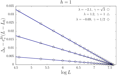
Figure 6: Numerical check of the term of order $O(L^{-1}\log L)$ in the expansion of Eq. (43) for the FCS of the staggered magnetization along the critical line $h=1$. We plot $\Delta_{s}$ (defined in Eq. (94)) with $L_{0}=2000$, substracting $c_{s}^{\rm fit}(L-L_{0})$, and taking for $c_{s}^{\text{fit}}$ the values collected in the corresponding column of Table 1. The dots correspond to $\Delta_{s}$ obtained by computing numerically $\chi_{\mathfrak{M}_{s}}(\lambda)$ from Eq. (39). The lines represent $d_{s}\log(L/L_{0})$, where $d_{s}$ is the coefficient of the $O(L^{-1}\log L)$ term predicted in Eq. (45).

3. Numerical check of the subleading term in the number of domain walls (Eq. (60) and Fig. 3)— In Fig. 3, we study numerically the presence of the $O(L^{-1}\log L)$ term (60) in the expansion of $\log\chi_{\mathfrak{K}}(\lambda)$. For this purpose, we consider the quantity

$$\Delta_{\mathfrak{K}}=L[\log\chi_{\mathfrak{K}}(\lambda)-a_{\mathfrak{K}}L-b_{\mathfrak{K}}\log L-c_{\mathfrak{K}}]\\ -L_{0}[\log\chi_{\mathfrak{K}}(\lambda)|_{L=L_{0}}-a_{\mathfrak{K}}L_{0}-b_{\mathfrak{K}}\log L_{0}-c_{\mathfrak{K}}],$$ (96)

where $a_{\mathfrak{K}}$, $b_{\mathfrak{K}}$, $c_{\mathfrak{K}}$ are the coefficients of the linear, logarithmic and $O(1)$ terms in the expansion of $\log\chi_{\mathfrak{K}}(\lambda)$, which can be determined from Eq. (70), and $\log\chi_{\mathfrak{K}}(\lambda)|_{L=L_{0}}$ is the FCS evaluated at an interval of length $L_{0}$. Therefore, if Eq. (60) is the $O(L^{-1}\log L)$ term in the expansion of $\log\chi_{\mathfrak{K}}(\lambda)$, then

$$\Delta_{\mathfrak{K}}\sim d_{\mathfrak{K}}\log(L/L_{0})$$ (97)

for large $L$, with $d_{\mathfrak{K}}$ the coefficient predicted in Eq. (60), as we actually observe in Fig. 3.

4. The derivation of the domain wall symbol (Eq. (56)).— Applying Eq. (10), we obtain after a little massage

$$\chi_{\mathfrak{K}}(\lambda) =e^{\lambda L}\sqrt{\det e^{-Y}}\det(P_{+}+G_{ba}P_{-})$$

$$=e^{\lambda L}\sqrt{\det e^{-Y}}\det P_{+}\det(I_{L+1}+G_{ba}P_{-}P_{+}^{-1})$$ (98)

where $P_{\pm}=\frac{1}{2}(T_{22}^{-1}-X\pm I_{L+1})$ and $I_{L+1}$ is the $L+1$-dimensional identity matrix. The matrix $e^{-Y}=T_{22}$ is tridiagonal,

$$\left[\begin{array}[]{ccccc}\cosh^{2}(\lambda)&-\frac{\sinh(2\lambda)}{2}&\cdots&0&0\\ -\frac{\sinh(2\lambda)}{2}&\cosh(2\lambda)&\cdots&0&0\\ \vdots&\vdots&\ddots&\vdots&\vdots\\ 0&0&0&\cosh(2\lambda)&-\frac{\sinh(2\lambda)}{2}\\ 0&0&0&-\frac{\sinh(2\lambda)}{2}&\cosh^{2}(\lambda)\end{array}\right],$$

while the matrix $P_{+}$ is triangular,

$$\left[\begin{array}[]{ccccc}1&0&0&\cdots&0\\ \tanh(\lambda)&1&0&\cdots&0\\ \tanh^{2}(\lambda)&\tanh(\lambda)&1&\cdots&0\\ \vdots&\vdots&\vdots&\ddots&\vdots\\ \tanh^{L}(\lambda)&\tanh^{L-1}(\lambda)&\tanh^{L-2}(\lambda)&\cdots&1\end{array}\right],$$

and $P_{-}=P_{+}-I_{L+1}$. Therefore, Eq. (C) simplifies to

$$\chi_{\mathfrak{K}}(\lambda)=e^{\lambda L}\cosh^{L}(\lambda)\det(I_{L+1}+G_{ba}P_{-}P_{+}^{-1}).$$ (99)

Taking now into account that $(P_{-}P_{+}^{-1})_{nm}=\delta_{n,m+1}\tanh(\lambda)$, we have that $I_{L+1}+G_{ba}P_{-}P_{+}^{-1}$ is the matrix

$$\left[\begin{array}[]{ccc|c}1+g_{-1}\tanh(\lambda)&\cdots&g_{-L}\tanh(\lambda)&0\\ g_{0}\tanh(\lambda)&\cdots&g_{-L+1}\tanh(\lambda)&0\\ \vdots&\ddots&\vdots&\vdots\\ g_{L-2}\tanh(\lambda)&\cdots&1+g_{-1}\tanh(\lambda)&0\\ \hline\cr g_{L-1}\tanh(\lambda)&\cdots&g_{0}\tanh(\lambda)&1\end{array}\right],$$

with $g_{n-m}=(G_{ba})_{nm}$. Hence, we can write (99) as

$$\chi_{\mathfrak{K}}(\lambda)=\det G_{\mathfrak{K}},$$ (100)

where $G_{\mathfrak{K}}$ is the $L\times L$ matrix with entries

$$(G_{\mathfrak{K}})_{nm}=\int_{0}^{2\pi}\frac{d\phi}{2\pi}g_{\mathfrak{K}}(\phi)e^{i\phi(n-m)},\quad n,m=1,\dots,L,$$

with $g_{\mathfrak{K}}(\phi)$ as in Eq. (56).

5. The derivation of the EFP in the $x$-direction for the Ising spin chain (Eq. (59)).— At $\gamma=1$, see Eq. (56), the logarithm of the EFP in the $x$-direction is given by

$$\log\mathcal{E}_{x}(h)=L(F(h)-\log 2)+O(1),$$

where $F(h)$ is the integral

$$F(h)=\int_{0}^{2\pi}\frac{d\phi}{2\pi}\log\left(1-\frac{he^{-i\phi}-1}{\sqrt{1+h^{2}-2h\cos\phi}}\right).$$ (101)

We then consider the derivative with respect to $h$ of Eq. (101) and continue analytically the integrand to the complex plane of $z=e^{i\phi}$. We end up with

$$F^{\prime}(h)=\frac{1}{2\pi i}\oint_{C}dz~{}f(z),$$ (102)

where the function $f(z)$ is given by

$$f(z)=\frac{1-z^{2}}{2z(hz-1)\left(z-h+z\sqrt{\frac{(h-z)(hz-1)}{z}}\right)},$$ (103)

and the contour $C$ is a circumference of unit radius encircling the origin anticlockwise, Fig. 7. For $h>1$, the domain of analyticity of $f$ is the complex plane with cuts along the segments $(0,1/h)$ and $(h,\infty)$.

Figure 7: Contours in the complex $z$-plane discussed in the main text.

The contour $C$ can be then deformed into $C^{\prime}$ depicted in Fig. 7 without crossing any singularities. One obtains the integral representation

$$F^{\prime}(h)=\int_{h}^{\infty}\frac{dx}{\pi}\frac{1}{2h\sqrt{x(x-h)(hx-1)}}=\frac{1}{\pi h^{2}}K(h^{-2}),$$ (104)

with $K(y)$ the complete elliptic integral of the first kind, written in Mathematica conventions. By integrating back Eq. (104) with respect to $h$ and observing that $F(\infty)=0$, see Eq. (101), the first line of Eq. (59) follows. An analogous calculation can be also performed for $h<1$. In this case, however, when deforming the contour, one shall extract the pole contribution at $z=1/h$ of $f(z)$ in Eq. (103). Finally, the critical EFP is obtained by taking the $h\rightarrow 1$ limit, which is well defined.

References

- (1) W. Feller, An introduction to probability theory and its applications Volume I, Wiley, 3rd ed., (1968).
- (2) I. Bloch, J. Dalibard, and W. Zwerger, Many-body physics with ultracold gases, Rev. Mod. Phys. 80, 885 (2008).
- (3) J. Armijo, T. Jacqmin, K. V. Kheruntsyan, and I. Bouchoule, Probing Three-Body Correlations in a Quantum Gas Using the Measurement of the Third Moment of Density Fluctuations, Phys. Rev. Lett. 105, 230402 (2010).
- (4) T. Jacqmin, J. Armijo, T. Berrada, K. V. Kheruntsyan, and I. Bouchoule, Sub-Poissonian Fluctuations in a 1D Bose Gas: From the Quantum Quasicondensate to the Strongly Interacting Regime, Phys. Rev. Lett. 106, 230405 (2011).
- (5) M. Gring, M. Kuhnert, T. Langen, T. Kitagawa, B. Rauer, M. Schreitl, I. Mazets, D. Adu Smith, E. Demler and J. Schmiedmayer, Relaxation and prethermalization in an isolated quantum system, Science 337, 1318 (2012).
- (6) P. Deift, A. Its, and I. Krasovsky, Toeplitz Matrices and Toeplitz Determinants under the Impetus of the Ising Model: Some History and Some Recent Results, Comm. Pure Appl. Math. 66, 1360 (2013).
- (7) M. L. Mehta, Random Matrices, vol. 142 of Pure and Applied Mathematics, Academic Press, 3rd ed. (2004).
- (8) V. Korepin, N. Bogoliubov and A. Izergin, Quantum Inverse Scattering and Correlation Functions, Cambridge University Press, Cambridge UK (1993).
- (9) G. Mussardo, Statistical Field Theory, Oxford University Press, 2nd ed. (2020).
- (10) R. W. Cherng and E. Demler, Quantum Noise Analysis of Spin Systems Realized with Cold Atoms, New J. Phys. 9, 7 (2007).
- (11) A. Lamacraft and P. Fendley, Order parameter statistics in the critical quantum Ising chain, Phys. Rev. Lett. 100, 165706 (2008).
- (12) M. Kormos, G. Mussardo, and A. Trombettoni, Expectation Values in the Lieb-Liniger Bose Gas, Phys. Rev. Lett. 103, 210404 (2009).
- (13) A. G. Abanov, D. A. Ivanov, and Y. Qian, Quantum fluctuations of one-dimensional free fermions and Fisher Hartwig formula for Toeplitz determinants, J. Phys. A: Math. Theor. 44, 485001 (2011).
- (14) D. A. Ivanov and A. G. Abanov, Characterizing correlations with full counting statistics: classical Ising and quantum XY spin chains, Phys. Rev. E 87, 022114 (2013).
- (15) K. Najafi and M. Rajabpour, Full Counting Statistics of subsystem energy in the free fermions and the quantum spin chain, Phys. Rev. B 96, 235109 (2017).
- (16) J.-M. Stéphan and F. Pollmann, Full counting statistics in the Haldane-Shastry chain, Phys. Rev. B 95, 035119 (2017).
- (17) A. Bastianello, L. Piroli, and P. Calabrese, Exact local correlations and full counting statistics for arbitrary states of the one-dimensional interacting Bose gas, Phys. Rev. Lett. 120, 190601 (2018).
- (18) M. Arzamasovs and D. Gangardt, Full counting statistics and large deviations in thermal 1D Bose gas , Phys. Rev. Lett. 122, 120401 (2019).
- (19) M. N. Najafi and M. A. Rajabpour, Formation probabilities and statistics of observables as defect problems in the free fermions and the quantum spin chains, Phys. Rev. B 101, 165415 (2020).
- (20) P. Calabrese, M. Collura, G. Di Giulio, and S. Murciano, Full counting statistics in the gapped XXZ spin chain, EPL 129, 60007 (2020).
- (21) V. Eisler, Universality in the Full Counting Statistics of Trapped Fermions, Phys. Rev. Lett. 111, 080402 (2013).
- (22) V. Eisler and Z. Rácz, Full Counting Statistics in a Propagating Quantum Front and Random Matrix Spectra, Phys. Rev. Lett. 110, 060602 (2013).
- (23) I. Lovas, B. Dóra, E. Demler, and G. Zaránd, Full counting statistics of time of flight images, Phys. Rev. A 95, 053621 (2017).
- (24) A. De Luca, J. Viti, D. Bernard, and B. Doyon, Nonequilibrium thermal transport in the quantum Ising chain, Phys. Rev. B 88, 134301 (2013).
- (25) M. Collura, F. H. L. Essler, and S. Groha, Full counting statistics in the spin-1/2 Heisenberg XXZ chain, J. Phys. A: Math. Theor. 50, 414002 (2017).
- (26) S. Groha, F. H. L. Essler, and P. Calabrese, Full Counting Statistics in the Transverse Field Ising Chain, SciPost Phys. 4, 043 (2018).
- (27) M. Collura, Relaxation of the order-parameter statistics in the Ising quantum chain, SciPost Phys. 7, 072 (2019).
- (28) G. Perfetto and A. Gambassi, Dynamics of large deviations in the hydrodynamic limit: Non-interacting systems, Phys. Rev. E 102, 042128 (2020).
- (29) O. Gamayun, O. Lychkovskiy, and J.-S. Caux, Fredholm determinants, full counting statistics and Loschmidt echo for domain wall profiles in one-dimensional free fermionic chains, SciPost Phys. 8, 036 (2020).
- (30) O. Gamayun, N. Iorgov, and Y. Zhuravlev, Effective free-fermionic form factors and the XY spin chain, SciPost Phys. 10, 070 (2021).
- (31) N. Smith, P. Le Doussal, S. Majumdar, and G. Schehr, Counting statistics for non-interacting fermions in a d-dimensional potential, Phys. Rev. E 103, L030105 (2021).
- (32) J-M. Stéphan, Emptiness formation probability, Toeplitz determinants, and conformal field theory, J. Stat. Mech.: Theory Exp. (2014) P05010.
- (33) I. Klich and L. Levitov, Many-Body Entanglement: a New Application of the Full Counting Statistics, Adv. Theor. Phys. 1134, 36 (2009).
- (34) H. F. Song, C. Flindt, S. Rachel, I. Klich, and K. Le Hur, Entanglement from Charge Statistics: Exact Relations for Many-Body Systems, Phys. Rev. B 83, 161408(R) (2011).
- (35) F. Song, S. Rachel, C. Flindt, I. Klich, N. Laflorencie, and K. Le Hur, Bipartite Fluctuations as a Probe of Many-Body Entanglement, Phys. Rev. B 85, 035409 (2012).
- (36) P. Calabrese, M. Mintchev, and E. Vicari, Exact relations between particle fluctuations and entanglement in Fermi gases, EPL 98, 20003 (2012).
- (37) D. Bernard and B. Doyon, Energy flow in non-equilibrium conformal field theory, J. Phys. A: Math. Theor. 45, 362001 (2012).
- (38) F. Franchini and A. Abanov, Asymptotics of Toeplitz determinants and the emptiness formation probability for the XY spin chain, J. Phys. A: Math. Gen. 38, 5069 (2005).
- (39) E. Lieb, T. Schultz, and D. Mattis, Two soluble models of an antiferromagnetic chain, Ann. Phys. 16, 407 (1961).
- (40) O. Gamayun, N. Iorgov, and O. Lisovyy, How instanton combinatronics solves Painlevé VI, V and III’s, J. Phys A: Math. Theor. 46, 335203 (2013).
- (41) F. Ares and J. Viti, Emptiness formation probability and Painlevé V equation in the XY spin chain, J. Stat. Mech.: Theory Exp. (2020) 013105.
- (42) V. Korepin, A. Izergin, F. Essler, and D. Uglov, Correlation functions of the spin 1/2 XXX antiferromagnet, Phys. Lett. A 190, 182 (1994).
- (43) K. Najafi and M. A. Rajabpour, Formation probabilities and Shannon information and their time evolution after quantum quench in the transverse-field XY chain, Phys. Rev. B 93, 125139 (2016).
- (44) F. Ares, M. A. Rajabpour, and J. Viti, Scaling of the Formation Probabilities and Universal Boundary Entropies in the Quantum XY chain, J. Stat. Mech.: Theory Exp. (2020) 083111.
- (45) I. Peschel, Calculation of reduced density matrices from correlation functions, J. Phys. A: Math. Gen. 36, L205 (2003).
- (46) T. Bartel, M-C. Chung, and U. Schollwoeck, Entanglement scaling in critical two-dimensional fermionic and bosonic systems, Phys. Rev. A 74, 022329 (2006).
- (47) S. Caracciolo, A. D. Sokal, and A. Sportiello, Algebraic/combinatorial proofs of Cayley-type identities for derivatives of determinants and pfaffians, Adv. Appl. Math. 50, 474 (2013).
- (48) R. Balian and E. Brezin, Nonunitary Bogoliubov transformations and extension of Wick’s theorem, Nuovo Cimento B (1965-1970) 64, 37 (1969).
- (49) L. Onsager, Crystal Statistics. I. A Two-Dimensional Model with an Order-Disorder Transition, Phys. Rev. 65, 117 (1944).
- (50) T. Schultz, D. Mattis, and E. Lieb, Two-Dimensional Ising Model as a Soluble Problem of Many Fermions, Rev. Mod. Phys. 36, 856 (1964).
- (51) G. Szegő, On certain hermitian forms associated with the Fourier series of a positive function, Festschrift Marcel Riesz, Lund (1952), 228–238
- (52) M. E. Fisher and R. E. Hartwig, Toeplitz determinants, some applications, theorems and conjectures, Adv. Chem. Phys. 15, 333 (1968).
- (53) J. Cardy, Boundary conditions, fusion rules and the Verlinde formula, Nucl. Phys. B 324, 581 (1989).
- (54) V. Eisler, Z. Rácz, and F. van Wijland, Magnetization distribution in the transverse Ising chain with energy flux, Phys. Rev. E 67, 056129 (2003).
- (55) T. Claeys, A. Its, and I. Krasovsky, Emergence of a singularity for Toeplitz determinants and Painlevé V, Duke Math. J. 160, 207 (2011).
- (56) M. Jimbo, Monodromy problem and the boundary condition for some Painlevé equations, Publ. RIMS, Kyoto Univ. 18, 1137 (1982).
- (57) M. Shiroishi, M. Takahashi, and Y. Nishiyama, Emptiness formation probability for the one-dimensional isotropic XY model, J. Phys. Soc. Japan 70, 3535 (2001).
- (58) N. Allegra, J. Dubail, J.-M. Stéphan, and J. Viti, Inhomogeneous field theory inside the arctic circle, J. Stat. Mech. (2016) 053108
- (59) H. Widom, Asymptotic Behavior of Block Toeplitz Matrices and Determinants, Adv. in Math. 13, 284 (1974).
- (60) H. Widom, Asymptotic Behavior of Block Toeplitz Matrices and Determinants II, Adv. in Math. 21, 1 (1976).
- (61) H. Widom, On the Limit of Block Toeplitz Determinants, Proceedings of the American Mathematical Society 50, 167 (1975).
- (62) F. Ares, J. G. Esteve, F. Falceto, and A. R. de Queiroz, Entanglement entropy in the long-range Kitaev chain, Phys. Rev. A 97, 062301 (2018).
- (63) M. Brockmann and J-M. Stéphan, Universal terms in the overlap of the ground state of the spin-1/2 XXZ chain with the Néel state, J. Phys. A: Math. Theor. 50, 354001 (2017).
- (64) H. Widom, The Strong Szegő limit theorem for circular arcs, Ind. Univ. Math. J. 21, 277 (1971).
- (65) J-M. Stéphan, G. Misguich, and F. Alet, Geometric entanglement of critical XXZ and Ising chains and Affleck-Ludwig boundary entropies, Phys. Rev. B 82, 180406(R) (2010).
- (66) A. M. Zagoskin and I. Affleck, Fermi Edge Singularities: Boundstates and Finite Size Effects, J. Phys. A: Math. Gen. 30, 5743 (1997).
- (67) J-M. Stéphan and J. Dubail, Local quantum quenches in critical one-dimensional systems: entanglement, the Loschmidt echo, and light-cone effects, J. Stat. Mech.: Theory Exp. (2011) 08019.
- (68) H. Boos and V. Korepin, Quantum Spin Chains and the Riemann zeta function with odd argument, J. Phys. A: Math. Gen. 34, 5311 (2001).
- (69) K. Najafi, M. A. Rajabpour, and J. Viti, Light-cone velocities after a global quench in a non-interacting model, Phys. Rev. B 97, 205103 (2018).
- (70) I. A. Ibraginov, On a theorem of Gabor Szegő, Mat. Zametki 3, 693 (1968) (In Russian, English translation: Math. Notes 3, 442 (1968)).
- (71) E. L. Basor, A localization theorem for Toeplitz determinants, Indiana Math. J. 28, 975 (1979).
- (72) K. K. Kozlowski, Truncated Wiener-Hopf operators with Fisher Hartwig singularities, arXiv:0805.3902.
- (73) E. L. Basor and C. A. Tracy, The Fisher-Hartwig conjecture and generalizations, Physica A 177, 167 (1991).
- (74) P. Deift, A. Its, and I. Krasovsky, Asymptotics of Toeplitz, Hankel, and Toeplitz+Hankel determinants with Fisher-Hartwig singularities, Ann. of Math. 174, 1243 (2011).
- (75) R.E. Hartwig and M. E. Fisher, Asymptotic behavior of Toeplitz matrices and determinants, Arch. Rational Mech. Anal. 32, 190 (1969).
- (76) N. M. Temme, Asymptotic Methods For Integrals, Series In Analysis, vol. 6. World Scientific, Singapore (2014).
- (77) N. G. Jones and R. Verresen, Asymptotic Correlations in Gapped and Critical Topological Phases of 1D Quantum Systems, J. Stat. Phys. 175, 1164 (2019).