Large-$N$ $SU(N)$ Yang–Mills theories with milder topological freezing

Abstract

We simulate $4d$ $SU(N)$ pure-gauge theories at large $N$ using a parallel tempering scheme that combines simulations with open and periodic boundary conditions, implementing the algorithm originally proposed by Martin Hasenbusch for $2d$ $CP^{N-1}$ models. That allows to dramatically suppress the topological freezing suffered from standard local algorithms, reducing the autocorrelation time of $Q^{2}$ up to two orders of magnitude. Using this algorithm in combination with simulations at non-zero imaginary $\theta$ we are able to refine state-of-the-art results for the large-$N$ behavior of the quartic coefficient of the $\theta$-dependence of the vacuum energy $b_{2}$, reaching an accuracy comparable with that of the large-$N$ limit of the topological susceptibility.

1 Introduction

The dependence of physical observables on the topological parameter $\theta$ is one of the most interesting properties of four dimensional $SU(N)$ pure-gauge theories. The parameter is coupled in the action to the topological charge

$$Q=\int d^{4}x\,q(x)=\frac{1}{64\pi^{2}}\varepsilon_{\mu\nu\rho\sigma}\int d^{4}x\,F^{a}_{\mu\nu}(x)F^{a}_{\rho\sigma}(x)\,;$$ (1)

$\theta$-dependence can be studied to achieve a better understanding of the non-perturbative features of Yang–Mills theories, but also has direct phenomenological implications for hadron physics in the limit of large number of colors ’t Hooft (1974, 1976); Witten (1979a, b); Veneziano (1979); Witten (1980); Di Vecchia and Veneziano (1980).

A particularly interesting quantity, whose dependence on $\theta$ has been thoroughly investigated, is the vacuum energy density $E(\theta)$, which is formally defined by the relation

$$E(\theta)\equiv-\frac{1}{V}\log\int[dA]e^{-S_{\mathit{YM}}[A]+i\theta Q[A]}\ ,$$ (2)

where $V$ is the four-dimensional euclidean space-time volume. The functional form of $E(\theta)$ is known only for very specific theories, like for QCD close to the chiral limit Di Vecchia and Veneziano (1980). It is customary to consider a Taylor expansion of $E(\theta)$ around $\theta=0$. Since $Q$ is odd under a $\mathrm{CP}$ transformation, only even powers of $\theta$ appear in the expansion, which can be parametrized in the form

$$E(\theta)-E(0)=\frac{1}{2}\chi\theta^{2}\left(1+\sum_{n=1}^{\infty}b_{2n}\theta^{2n}\right)\ .$$ (3)

The coefficients of this expansion are related to the cumulants of the topological charge distribution at $\theta=0$, for instance $\chi=\langle Q^{2}\rangle_{\theta=0}/V$, where $\chi$ is the topological susceptibility.

While the exact numerical values of the coefficients $\chi$ and $b_{2n}$ are generically unknown, something is known about their dependence on the number of colors $N$, at least when $N$ is large enough. Indeed, assuming that a non-trivial $\theta$-dependence is present in the large-$N$ limit, it is possible to fix the large $N$ scaling form of the energy density $E(\theta,N)=N^{2}\bar{E}(\theta/N)$ Witten (1979b, 1980, 1998), implying

$$\chi = \bar{\chi}+O\left(\frac{1}{N^{2}}\right),$$ (4)

$$b_{2n} = \frac{\bar{b}_{2n}}{N^{2n}}+O\left(\frac{1}{N^{2\left(n+1\right)}}\right)\ .$$ (5)

The value of $\bar{\chi}$ is related to the mass of the $\eta^{\prime}$ meson by the Witten–Veneziano formula Witten (1979b); Veneziano (1979), which provides the estimate $\bar{\chi}\simeq(180\,\text{MeV})^{4}$. Analytic estimates of $\bar{\chi}$ and of the $\bar{b}_{2n}$ coefficients are available only for two dimensional models D’Adda et al. (1978); Campostrini and Rossi (1991); Del Debbio et al. (2006); Rossi (2016); Bonati et al. (2016a). Given the non-perturbative nature of $\theta$-dependence, the numerical lattice approach is the natural tool to investigate such topics quantitatively, and in particular to test large-$N$ predictions Alles et al. (1997a, b); Del Debbio et al. (2005); Del Debbio et al. (2002a); D’Elia (2003); Del Debbio et al. (2006); Lucini et al. (2005a); Giusti et al. (2007); Vicari and Panagopoulos (2009); Panagopoulos and Vicari (2011); Cè et al. (2015, 2016); Bonati et al. (2016b, a, 2018, 2020). There are however some non-trivial computational challenges that have to be faced, especially in the large $N$ regime.

The first problem is related to the measure of the coefficients $b_{2n}$. The task is challenging by itself since, contrary to what happens for $\chi$, these coefficients approach zero as $N$ is increased. In addition, the simplest estimators available for $\theta=0$ simulations are based on the cumulants of the topological charge distribution, which are not self-averaging quantities, leading to a bad signal-to-noise ratio for large volumes. Such problem can be solved by introducing an explicit source term in the action, coupled to the topological charge density, which corresponds in practice to an imaginary $\theta$ term Bhanot and David (1985); Azcoiti et al. (2002); Alles and Papa (2008); Imachi et al. (2006); Aoki et al. (2008); Panagopoulos and Vicari (2011); Alles et al. (2014); D’Elia and Negro (2012, 2013); D’Elia et al. (2013). The method was exploited for the determination of the $b_{2n}$ coefficients first in Ref. Panagopoulos and Vicari (2011) and later developed and applied in several works to both $SU(N)$ Yang–Mills theory Bonati et al. (2016b, a, 2018, 2020) and two dimensional $CP^{N-1}$ models Bonanno et al. (2019); Berni et al. (2019).

The second problem is the so-called “freezing problem”, it represents a well known problem in a wide range of theories sharing the presence of topological excitations Alles et al. (1996); de Forcrand et al. (1998); Lucini and Teper (2001); Del Debbio et al. (2002a); Leinweber et al. (2004); Del Debbio et al. (2004); Lüscher and Schaefer (2011); Laio et al. (2016); Flynn et al. (2015); Bonati et al. (2016c); Bonati and D’Elia (2018); Athenodorou and Teper (2020) and it will be the main topic of this work. When adopting local update algorithms on lattices with periodic boundary conditions, the topological modes experience a severe critical slowing down when approaching the continuum limit, with the autocorrelation time of the topological charge which grows approximately exponentially as a function of $1/a$ Del Debbio et al. (2002a); Del Debbio et al. (2004). As a consequence gauge configurations stay fixed (frozen) in a given topological sector for an exceedingly large amount of Monte Carlo time, thus preventing a correct sampling of the path-integral distribution. This problem becomes even worse in the large-$N$ limit, since at fixed lattice spacing $a$ the autocorrelation time of the topological charge seems to grow exponentially with the number of colors Del Debbio et al. (2002a); Del Debbio et al. (2004); Bonanno et al. (2019).

Despite the fact that a definitive solution to the topological freezing problem has been obtained only in toy models Bonati and D’Elia (2018), several strategies have been proposed to reduce its severeness, in particular by reducing the exponential critical slowing down to a polynomial critical slowing down Vicari (1993); Lüscher and Schaefer (2011); Laio et al. (2016); Bonati and D’Elia (2018), or to extract information even from completely frozen configurations Bietenholz et al. (2015). A popular method, proposed in Ref. Lüscher and Schaefer (2011), is to adopt open boundary conditions for the gauge fields in the time direction instead of the usual periodic ones. The presence of an open boundary eliminates barriers among different topological sectors even in the continuum, and one expects the critical slowing down of the topological modes to be essentially diffusive, with an autocorrelation time increasing as $1/a^{2}$ approaching the continuum limit. Using this method, however, one also breaks translation invariance and loses completely any notion of global topological charge. Therefore $\chi$ and $b_{2n}$ can only be estimated from the integral of the $(2n+2)$-point connected correlators of the topological charge density on the bulk of the lattice.

A different strategy, that keeps the advantages of the open boundary conditions without breaking translation invariance, has been proposed by M. Hasenbusch in Ref. Hasenbusch (2017), where it was tested for two dimensional $CP^{N-1}$ models. The basic idea of this method is to combine periodic and open boundary conditions in a parallel tempering framework, using the copies with open or partially open boundary conditions as sources of topological fluctuations for the copy with periodic boundary conditions, which is the one on which measures are performed. To reduce the number of copies to be used in the parallel tempering, open boundary conditions are not enforced along all the temporal boundaries, but only in a limited space region, that will be referred to as the “defect” in the following.

In Ref. Berni et al. (2019) it was shown that in two dimensional $CP^{N-1}$ models, for large $N$ values, the adoption of the Hasenbusch algorithm in combination with the imaginary-$\theta$ method allows to achieve impressive improvements compared to previously available results for the $\theta$-dependence of these models. The aim of the present work is to test the same setup in the case of four dimensional $SU(N)$ Yang–Mills theories at zero temperature, comparing its performance with that of the standard simulations. In doing this we will also refine the state-of-the-art results about the large-$N$ behavior of the $b_{2}$ coefficient.

This paper is organized as follows: in Sec. 2 we discuss our lattice setup, along with the parallel tempering algorithm and the imaginary-$\theta$ method, in Sec. 3 we show the numerical results obtained with the parallel tempering and finally in Sec. 4 we draw our conclusions.

2 Lattice setup

In this section we introduce the discretizations adopted for the action and the topological charge, we present a summary of the imaginary-$\theta$ method and discuss the parallel tempering algorithm employed in our simulations.

2.1 Lattice action and lattice topological charge

We discretize the Yang–Mills action on an hyper-cubic lattice of size $L$ and with periodic boundary conditions in every direction (see Sec. 2.3 for the defect) using the standard Wilson action:

$$S_{W}=-\frac{\beta}{N}\sum_{x,\mu>\nu}\Re\mathrm{Tr}\left\{\Pi_{\mu\nu}(x)\right\},$$ (6)

where $\Pi_{\mu\nu}(x)\equiv U_{\mu}(x)U_{\nu}(x+\hat{\mu})U_{\mu}^{\dagger}(x+\hat{\nu})U_{\nu}^{\dagger}(x)$ is the plaquette operator.

For the topological charge (1), we adopt the simplest discretization with definite parity, the so-called clover discretization:

$$Q_{\mathit{clov}}=\frac{1}{2^{9}\pi^{2}}\sum_{x,\mu,\nu,\rho,\sigma}\varepsilon_{\mu\nu\rho\sigma}\mathrm{Tr}\left\{C_{\mu\nu}(x)C_{\rho\sigma}(x)\right\},$$ (7)

where $C_{\mu\nu}(x)$ is a discretization of the field strength given by the sum of all the 4 plaquettes centered in the site $x$ and lying on the $\mu$–$\nu$ plane. $Q_{\mathit{clov}}$ is generically non-integer and it is related, configuration by configuration, to the physical charge $Q$ by Campostrini et al. (1988):

$$Q_{\mathit{clov}}=ZQ+\eta,$$ (8)

where $Z$ is a finite renormalization constant that approaches 1 in the continuum limit, and $\eta$ is a stochastic noise due to ultraviolet (UV) fluctuations at the scale of the lattice spacing. Using the variance of $Q_{\mathit{clov}}$ to estimate the topological susceptibility would require to take into account both multiplicative and additive renormalizations, which can be avoided by using one of the several smoothing procedures that have been proposed in the literature, such as the gradient flow Lüscher (2010a, b) or cooling Berg (1981); Iwasaki and Yoshie (1983); Itoh et al. (1984); Teper (1985); Ilgenfritz et al. (1986); Campostrini et al. (1990); Alles et al. (2000), which are all known to agree with each other when properly matched Bonati and D’Elia (2014); Alexandrou et al. (2015). In this work we use cooling due to its simplicity and numerical effectiveness.

We denote by $Q_{\mathit{clov}}^{\mathit{cool}}$ the topological charge obtained by measuring the observable Eq. (7) on a configuration to which a certain number of cooling steps have been applied. To assign an integer topological charge $Q_{L}$ to each configuration we follow Ref. Del Debbio et al. (2002a), defining

$$Q_{L}=\mathrm{round}\left\{\alpha\,Q_{\mathit{clov}}^{\mathit{cool}}\right\},$$ (9)

where “$\mathrm{round}$” denotes the rounding to the closest integer and the value of $\alpha$ is fixed by minimizing

$$\braket{\left(\alpha\,Q_{\mathit{clov}}^{\mathit{cool}}-\mathrm{round}\left\{\alpha\,Q_{\mathit{clov}}^{\mathit{cool}}\right\}\right)^{2}}\ ,$$ (10)

so that the maxima in the distribution of $\alpha Q_{\mathit{clov}}^{\mathit{cool}}$ are located approximately at integer values; such fixing is performed at $\theta=0$ and then adopted also for $\theta\neq 0$. The topological susceptibility computed using $Q_{L}$ becomes stable (i.e. independent of the number of cooling steps $n_{\mathit{cool}}$) after $n_{\mathit{cool}}\sim 10$, moreover such threshold reveals to be weakly dependent on the lattice spacing, thus we chose $n_{\mathit{cool}}=20$ to define the topological charge in all simulations, verifying also the stability of all continuum extrapolations if a different value of $n_{\mathit{cool}}$ is used.

2.2 Imaginary-$\theta$ method

As anticipated in the introduction, the imaginary-$\theta$ method is a technique that is useful to estimate the topological susceptibility and especially the coefficients $b_{2n}$ introduced in Eq. (3). In this section we provide a short summary of this computational method, referring to Ref. Bonati et al. (2016b) for more details. The idea of the method is to introduce an imaginary $\theta$ term, in order to avoid a sign problem, and to extract $\chi$ and $b_{2n}$ from the dependence on $\theta$ of the cumulants of the topological charge distribution: the method wins over the standard computation at $\theta=0$ since now the information on the $b_{2n}$ parameters is contained in all cumulants, including the lowest order ones. The procedure is most conveniently explained by working formally in the continuum: the continuum euclidean action can be written in the form

$$S(\theta_{I})=S_{\mathit{YM}}-\theta_{I}Q,$$ (11)

where $\theta_{I}=i\theta$. The dependence on $\theta_{I}$ of the cumulants of the topological charge distribution can be computed from the derivatives of $E(\theta)$ in Eq. (2), properly continued to the imaginary axis, and can be expressed in terms of $\chi$ and $b_{2n}$ using Eq. (3). As an example, the explicit expressions of the first few cumulants as a function of $\theta_{I}$ read:

$$\begin{split}\frac{k_{1}(\theta_{I})}{V}&=\chi\left[\theta_{I}-2b_{2}\theta_{I}^{3}+3b_{4}\theta_{I}^{5}+O(\theta_{I}^{6})\right],\\ \frac{k_{2}(\theta_{I})}{V}&=\chi\left[1-6b_{2}\theta_{I}^{2}+15b_{4}\theta_{I}^{4}+O(\theta_{I}^{5})\right],\\ \frac{k_{3}(\theta_{I})}{V}&=\chi\left[-12b_{2}\theta_{I}+60b_{4}\theta_{I}^{3}+O(\theta_{I}^{4})\right],\\ \frac{k_{4}(\theta_{I})}{V}&=\chi\left[-12b_{2}+180b_{4}\theta_{I}^{2}+O(\theta_{I}^{3})\right],\end{split}$$ (12)

where $V$ is the space-time volume and the first fourth cumulants of the topological charge are

$$\begin{split}k_{1}&=\braket{Q},\\ k_{2}&=\braket{Q^{2}}-\braket{Q}^{2},\\ k_{3}&=\braket{Q^{3}}-3\braket{Q^{2}}\braket{Q}+2\braket{Q}^{3},\\ k_{4}&=\braket{Q^{4}}-4\braket{Q^{3}}\braket{Q}-3\braket{Q^{2}}^{2}\\ &\quad\,+12\braket{Q^{2}}\braket{Q}^{2}-6\braket{Q}^{4}.\end{split}$$ (13)

All these averages are computed by using the weight $e^{-S(\theta_{I})}$ in the path-integral.

Let us now describe what changes on the lattice: the lattice action is

$$S_{L}(\theta_{L})=S_{W}-\theta_{L}Q_{\mathit{clov}},$$ (14)

where the $\theta$-term is discretized by using the non-smoothed clover charge $Q_{\mathit{clov}}$ defined in the previous subsection, and $\theta_{L}$ is the bare imaginary-$\theta$ coupling. The reason for using $Q_{\mathit{clov}}$ is that with this choice standard heatbath and overrelaxation algorithms can be used in the update. Relations analogous to Eq. (12) can be obtained, where $\theta_{I}=Z\theta_{L}$ and $Z$ is the renormalization constant appearing in Eq. (8). Measuring the cumulants for several values of $\theta_{L}$ we can thus fit the values of $\chi$, $b_{2n}$ and $Z$. We explictly note that the cumulants are not affected by the renormalization of $Q_{\mathit{clov}}$ since they are evaluated by using the smoothed and rounded charge $Q_{L}$ introduced in the previous section (see Ref. Berni et al. (2019) for a more detailed discussion on this point).

2.3 Parallel tempering of volume defect

The lattice action in Eq. (14), as the standard Wilson action, is linear in each of the link variables, hence standard heathbath Creutz (1980); Kennedy and Pendleton (1985) and overrelaxation Creutz (1987) algorithms can be applied to update the gauge configurations when using the imaginary-$\theta$ method. However, as anticipated in the introduction, the local nature of this updating procedure results in a slowing down of the topological modes, which is exponential both in the inverse lattice spacing and in the number $N$ of colors. This makes very difficult to perform controlled continuum extrapolations for large values of $N$, since even simulations with moderately small values of the lattice spacing become prohibitively expensive as $N$ is increased.

To mitigate this problem, we adopt, in this work, the parallel tempering algorithm proposed for the $CP^{N-1}$ models in Ref. Hasenbusch (2017), where this algorithm has been shown to perform as well as simulations with open boundaries while bypassing their complications related to finite-size effects. Moreover, as shown for $CP^{N-1}$ models in Ref. Berni et al. (2019), parallel tempering can be easily applied in combination with the imaginary-$\theta$ method discussed in the previous subsection.

In this algorithm we consider $N_{r}$ identical systems, differing only for the boundary conditions on a cuboid defect located on a given spatial slice. In particular, the boundary conditions imposed on the links that orthogonally cross the defect are chosen so that the different copies interpolate between periodic boundary conditions (pbc) and open boundary conditions (obc). Each system is evolved independently using standard local algorithms, and different copies are exchanged from time to time with a Metropolis step, so that the strong reduction of the autocorrelation time achieved in the obc copy is transferred to the pbc one, on which the measure of the cumulants of the topological charge $Q_{L}$ is performed. Since the injection (or ejection) of topological charge in the system is mainly triggered by the update of the links close to the defect, it is convenient Hasenbusch (2017) to alternate updating sweeps over the whole lattice with hierarchic updates over sub-regions of the lattice centered around the defect. In particular, we updated more frequently small hyper-rectangular regions centered around the defect.

In our simulations the location of the defect is the tridimensional region

$$\begin{aligned} D=\Big{\{}&x_{1}=L-a,\,0\leq x_{2}<L_{d}^{(2)},\,\\ &0\leq x_{3}<L_{d}^{(3)},\,0\leq x_{4}<L_{d}^{(4)}\Big{\}},\end{aligned}$$

however, after every hierarchic update, we perform a random translation of the pbc copy by one lattice spacing, thus effectively moving the location of the defect. For the sake of the simplicity we use a cubic defect $L_{d}^{(2)}=L_{d}^{(3)}=L_{d}^{(4)}\equiv L_{d}$ and it is sufficient to choose $L_{d}$ equal to a few lattice spacings to obtain satisfactory performances. For a discussion on how the choice of $L_{d}$ affects the efficiency of the algorithm, see Sec. 3.1.

In order to specify how the different boundary conditions across the defect are implemented, it is convenient to rescale each link of every replica according to

$$U^{(r)}_{\mu}(x)\to K_{\mu}^{(r)}(x)U^{(r)}_{\mu}(x),$$

where $U_{\mu}^{(r)}(x)$ indicates a link of the $r^{\text{th}}$ replica and the explicit expression of $K^{(r)}_{\mu}(x)$ is:

$$K_{\mu}^{(r)}(x)=\begin{cases}c(r),\quad&\mbox{ if}\quad\mu\neq 1\ \mathrm{and}\ x\in D,\\ 1,\quad&\mbox{ otherwise,}\end{cases}$$

so that only the links crossing the volume defect are affected by its presence. For the pbc replica (corresponding to $r=0$) we have $c(0)=1$, for the obc replica (corresponding to $r=N_{r}-1$) we have $c(N_{r}-1)=0$, for $0<r<N_{r}-1$ the value of $c(r)$ interpolates between 0 and 1. With these notations the action of the $r^{\text{th}}$ copy reads

$$S_{L}^{(r)}(\theta_{L})= \,\,S_{W}^{(r)}+S_{\theta}^{(r)}(\theta_{L})$$

$$= -\frac{\beta}{N}\sum_{x,\mu>\nu}K^{(r)}_{\mu\nu}(x)\Re\mathrm{Tr}\left\{\Pi^{(r)}_{\mu\nu}(x)\right\}$$

$$-\theta_{L}Q_{\mathit{clov}}\left[U_{\mu}^{(r)}(x)\right],$$

where $K^{(r)}_{\mu\nu}(x)$ is a short-hand for

$$K^{(r)}_{\mu\nu}(x)\equiv K^{(r)}_{\mu}(x)K^{(r)}_{\nu}(x+\hat{\mu})K^{(r)}_{\mu}(x+\hat{\nu})K^{(r)}_{\nu}(x).$$

Note that we chose to keep the $\theta$ term insensitive to the presence of the defect, which only affects the Wilson part of the action. Exploratory simulations performed by modifying also the $\theta$ term provided evidence that this choice does not significantly affects the performance of the algorithm, analogously to what was found for $CP^{N-1}$ models in Ref. Berni et al. (2019). This is not surprising since the barriers between the topological sectors, responsible of the critical slowing down, stem essentially from the Wilson term.

The swap of replicas was proposed after every step of hierarchic update, for every couple of adjacent copies $r$ and $r+1$ (differentiating the cases of even and odd $r$ in order to avoid synchronization problems), and was accepted with the Metropolis probability

$$\begin{aligned} p=&\min\left\{1,\exp\left\{-\Delta S\right\}\right\}\\ =&\min\left\{1,\exp\left\{-S_{W}^{\mathit{swap}}+S_{W}^{\mathit{no\,swap}}\right\}\right\},\end{aligned}$$ (15)

where the $\theta$-term, which is not affected by the defect, does not enter the acceptance probability. Since boundary conditions of different replicas differ only on a sub-region of the lattice, to compute $\Delta S$ it is sufficient to sum the contributions to the action of the plaquettes centered on sites lying in a hyper-cuboid region centered around the defect and extending one lattice spacing from it.

For the parallel tempering to be effective in decorrelating the topological modes of the pbc copy there must be no bottleneck for a configuration in the obc copy to be swapped toward the pbc one. In order to guarantee a random walk without barrier of the configurations between the different replicas it is thus convenient to choose the constants $c(r)$ entering $K^{(r)}_{\mu}(x)$ in such a way that the acceptance ratio is constant for all the proposed swaps: $p(0,1)=p(1,2)=\cdots=p(N_{r}-2,N_{r}-1)$.

3 Numerical results

In order to compare the performances of parallel tempering with the ones of the standard algorithm, we performed simulations for $N=4$ and $6$ with both algorithms and for several values of $\beta$ at $\theta_{L}=0$, measuring the autocorrelation time of $Q^{2}_{L}$. We then performed simulations at non-zero $\theta_{L}$ with parallel tempering for each value of $\beta$, to estimate $\chi$, $b_{2}$ and $b_{4}$ using the imaginary-$\theta$ method.

In Tab. 1 we summarize the parameters of the performed simulations. Lattice sizes have been chosen to ensure that $L\sqrt{\sigma}\gtrsim 3$, where $\sigma\simeq\left(440\text{ MeV}\right)^{2}$ is the string tension, so as to have finite-size effects under control Del Debbio et al. (2002b); Bonati et al. (2016a). Statistics reported in Tab. 1 refer to the parallel tempering simulations and are reported in number of parallel tempering steps. A single step of tempering update consists first of all of a complete update of each replica, using 5 lattice sweeps of over-relaxation Creutz (1987) followed by 1 lattice sweep of heat-bath Creutz (1980); Kennedy and Pendleton (1985), both implemented à la Cabibbo–Marinari Cabibbo and Marinari (1982), i.e., updating all the $N(N-1)/2$ diagonal $SU(2)$ subgroups of $SU(N)$. After this “global” update step we perform an iteration on the sub-lattices entering the hierarchical update (see Sec. 2.3), each iteration consisting of

• a local update sweep of the sub-lattices for every replica, using the same combination of local algorithms adopted for the global update;

• the parallel tempering swap proposal;

• a random translation of the pbc copy by one lattice spacing.

Since each system is updated using the same procedure and the time required for hierarchic updates, swap and translations is negligible with respect to the time of the global update, the total numerical effort of a single parallel tempering step is $\sim N_{r}$ times larger than the one required for the local update in the standard setup.

$N=4$
$\beta$	$L/a$	$a\sqrt{\sigma}$	$L\sqrt{\sigma}$	$\theta_{L}^{\mathit{max}}$	Stat. $\theta=0$	Stat. $\theta\neq 0$
11.104	16	0.1981(5)*	3.17	15	255k	787k
11.347	20	0.1590(6)	3.17	15	1.39M	2.44M
$N=6$
$\beta$	$L/a$	$a\sqrt{\sigma}$	$L\sqrt{\sigma}$	$\theta_{L}^{\mathit{max}}$	Stat. $\theta=0$	Stat. $\theta\neq 0$
24.768	12	0.2912(11)	3.57	15	103k	257k
24.845	12	0.2801(13)	3.41	15	113k	166k
25.056	12	0.2499(10)	3.04	15	228k	280k
25.394	14	0.2143(8)	3.00	15	513k	553k
25.750	16	0.1878(18)	3.00	17.5	1.12M	1.84M

Table 1: Summary of simulation parameters. Simulations at non-zero values of $\theta_{L}$ were performed in steps of $\Delta\theta_{L}=2$ up to $\theta_{L}=10$ and in steps of $\Delta\theta_{L}=2.5$ for $\theta_{L}>10$. The last column refers to the total statistics accumulated for all imaginary-$\theta$ simulations. The defect length was, in all cases, $L_{d}/a=2$. All simulations for $N=4$ were performed using $N_{r}=10$, corresponding to a constant swap probability $p$ around $20\%$, while simulations for $N=6$ used $N_{r}=17$, corresponding to $p\approx 30\%$. Lattice spacings are taken from Ref. Lucini et al. (2005b) or interpolation/extrapolation of data thereof, except for the one marked with *, which comes from Ref. Del Debbio et al. (2002b).

3.1 Parallel tempering: results and comparison

Figure 1: Monte Carlo time evolution of the lattice topological charge $Q_{L}$ for a run with $N=6$, $\beta=25.75$ and $\theta_{L}=0$. For the comparison to be fair, data for the parallel tempering case are plotted as a function of the total number of global updates performed on all the replicas, i.e. $17$ times the number of parallel tempering updates.

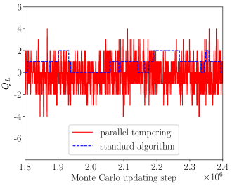
Just by inspection of the time histories of the topological charge it is simple to realize that parallel tempering substantially reduces the topological freezing allowing us to perform simulations at values of the lattice spacings which would have been otherwise prohibitive with the standard algorithm. An example of Monte Carlo time evolution of $Q_{L}$ obtained with parallel tempering for $N=6$, $\beta=25.75$ and $\theta_{L}=0$ is shown in Fig. 1, where we compare it with the evolution obtained with the standard algorithm.

In order to quantitatively characterize the gain achieved with parallel tempering and optimize its efficiency, it is useful to study the autocorrelation time of the topological susceptibility. We use as definition of the autocorrelation time for the generic observable $\mathcal{O}$ the expression Berg (2004)

$$\tau(\mathcal{O})=\frac{1}{2}\left(\frac{\Delta_{\mathcal{O}}^{\mathit{binned}}}{\Delta_{\mathcal{O}}^{\mathit{naive}}}-1\right)^{2},$$ (16)

where $\Delta_{\mathcal{O}}^{\mathit{binned}}$ is the error associated to $\langle\mathcal{O}\rangle$ by using a self-consistent binning analysis, while $\Delta_{\mathcal{O}}^{\mathit{naive}}$ is the usual standard error of the mean for independent identically distributed samples. The autocorrelation time of the topological susceptibility, however, does not take into account the increased computational effort of the parallel tempering algorithm with respect to the standard local algorithms. As a figure of merit for the computational effectiveness of parallel tempering, it is thus convenient to introduce the effective autocorrelation time given by

$$\tau_{\mathit{pt}}(\mathcal{O})=\tau(\mathcal{O})N_{r}\ .$$ (17)

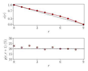
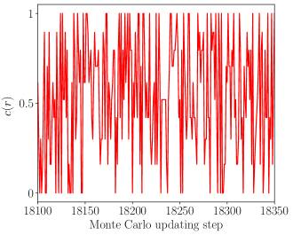
As discussed in the previous section, in every parallel tempering simulation we tuned the parameters $c(r)$ in such a way that the acceptance $p(r,r+1)$ of the Metropolis swap move between the replicas $r$ and $r+1$ is approximately independent of $r$. This tuning was performed using test simulations at $\theta_{L}=0$ (acceptances do not depend on $\theta_{L}$), and in Fig. 2 we show an example of the behavior of $c(r)$ for a run with $N=4$ and $\beta=11.347$. Deviations from the linear behavior appear to be small in the optimal $c(r)$ values, however using these values $\tau_{\mathit{pt}}(Q_{L}^{2})$ is about half the one obtained by using a simple linear interpolation. Once $p(r,r+1)$ is almost independent of $r$, configurations move freely among the different replicas following a random walk, as shown in Fig. 3.

The constant value $p$ that is reached by $p(r,r+1)$ after the tuning of $c(r)$ obviously depends on the number $N_{r}$ of replicas used. We did not perform a systematic investigation of the dependence on $p$ of the numerical effectiveness of parallel tempering, however this dependence seems to be quite mild. Indeed by increasing the number of replicas $N_{r}$, the constant acceptance probability $p$ grows and the autocorrelation time $\tau(Q_{L}^{2})$ is reduced, however also the computational cost increases with $N_{r}$. The net effect is that $\tau_{\mathit{pt}}(Q_{L}^{2})$ is largely insensitive to the specific value of $p$, at least as far as it is not too close to $0$ or $1$, as we verified in some test simulations. For example, simulations performed with $N=4$ and $\beta=11.104$ using $p\simeq 20\%$ (achieved with $N_{r}=10$) or $p\simeq 30\%$ (corresponding to $N_{r}=12$) provided consistent values of $\tau_{\mathit{pt}}(Q_{L}^{2})$: $72(10)$ and $78(18)$ respectively. The value of $p$ was kept fixed while approaching the continuum limit, and in all cases we found that this could be achieved by using the same value of $N_{r}$ for the different lattice spacings (at fixed physical volume).

Figure 2: Behavior of $c(r)$ as a function of the replica index $r$ compared to a simple linear behavior (figure above), along with the corresponding acceptances ($\sim 20\%$) for the swap between copies $r$ and $r+1$ (figure below). Data refer to a run with $N=4$, $\beta=11.347$ and $\theta_{L}=0$.

Figure 3: Random walk of a configuration among different replicas during a parallel tempering run for $N=4$, $\beta=11.347$ and $\theta_{L}=0$. Replicas are parametrized by their value of $c(r)$ and the Monte Carlo time is expressed in units of the parallel tempering update step defined in the text.

Most of the simulations reported in this work used $L_{d}/a=2$ for the size of the defect, a value that is sufficient to drastically reduce the freezing problem. To investigate the dependence of $\tau_{\mathit{pt}}$ on $L_{d}$ some more simulations have been performed with $L_{d}/a=3$ and $L_{d}/a=1$ for the case $N=6$, always keeping the swap acceptance probability $p$ fixed to about $30\%$, which requires to scale the number of replicas approximately as $\sim\sqrt{L_{d}^{3}}$.

$N=4$
$\beta$	$a\sqrt{\sigma}$	$L_{d}/a$	$p(\%)$	$N_{r}$	$\tau_{\mathit{pt}}\left(Q_{L}^{2}\right)$	$\tau_{\mathit{std}}\left(Q_{L}^{2}\right)$
$11.104$	$0.1981(5)$	$2$	20	10	72(10)	140(10)*
			30	12	78(18)
11.347	0.1590(6)	2	20	10	380(80)	1000(200)
$N_{c}=6$
$\beta$	$a\sqrt{\sigma}$	$L_{d}/a$	$p(\%)$	$N_{r}$	$\tau_{\mathit{pt}}\left(Q_{L}^{2}\right)$	$\tau_{\mathit{std}}\left(Q_{L}^{2}\right)$
24.768	0.2912(11)	2	30	17	16(3)	110(10)*
$24.845$	$0.2801(13)$	1	30	7	120(30)	220(30)*
		2		17	22(5)
		3		29	30(6)
25.056	0.2499(10)	2	30	17	39(8)	800(100)*
25.394	0.2143(8)	2	30	17	110(40)	5000(1500)
$25.750$	$0.1874(8)$	2	30	17	760(200)	$\sim 10^{5}$**
		3		30	43(11)

Table 2: Results for the autocorrelation time of $Q^{2}_{L}$ obtained by using the standard and the Hasenbusch algorithm. Quantities denoted with $*$ are taken from Ref. Bonati et al. (2016a), where the procedure used for the local update was the same of the present work. The result denoted by ** is just a rough estimate, since it was impossible to obtain a reliable value even after $\sim 2.5$M trajectories.

Figure 4: Scaling of $\tau_{\mathit{pt}}\left(Q^{2}_{L}\right)$ with the inverse lattice spacing obtained by using the local algorithms or parallel tempering for $N=6$. The scaling of the autocorrelation time obtained with the standard algorithm and with parallel tempering at fixed $L_{d}/a=2$ are both compatible with an exponential scaling in $1/a$ (dashed and solid line). Best fits performed with the fit function $\log\{\tau_{\mathit{pt}}\}=k_{0}+k_{1}/(a\sqrt{\sigma})$ yield $k_{1}=3.24(20)$ and $1.95(17)$ for the standard and the parallel tempering updates respectively.

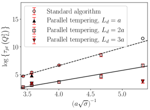
A complete list of the obtained autocorrelation times $\tau_{\mathit{pt}}(Q_{L}^{2})$ is reported in Tab. 2, where they are also compared with the results obtained in Ref. Bonati et al. (2016a) using just local algorithms. The scaling of $\tau_{\mathit{pt}}(Q_{L}^{2})$ with $1/(a\sqrt{\sigma})$ for the case $N=6$ is instead shown in Fig. 4.

Simulations performed for $N=6$ at $\beta=24.845$ (corresponding to the points at $1/(a\sqrt{\sigma})\simeq 3.57$ in Fig. 4) using $L_{d}/a=1,2,3$ show that $L_{d}/a=2$ is the optimal choice for this value of the coupling. As can be seen from Fig. 4, autocorrelation times extracted from simulations performed at fixed $L_{d}/a=2$ are much smaller than the corresponding ones obtained from simulation using local update algorithms, also for smaller values of the lattice spacing. However $\tau_{\mathit{pt}}(Q_{L}^{2})$ still seems to scale exponentially with the inverse lattice spacing. This is due to the fact that, by approaching the continuum limit at fixed $L_{d}/a$, the size of the defect in physical units is reduced, and the mechanism of injection of topological charge through the defect becomes less and less efficient.

If instead $L_{d}$ is kept fixed in physical units while approaching the continuum limit, one generically expects a polynomial critical slowing down in $1/(a\sqrt{\sigma})$. To investigate this point we performed additional simulations at $\beta=25.75$ using $L_{d}/a=3$, in order to have at this lattice spacing a defect of the same physical size as the one corresponding to $L_{d}/a=2$ at $\beta=24.845$ (in both the cases $L_{d}\sqrt{\sigma}\sim 0.56$). The outcome of this test is that, despite a $\approx 33\%$ reduction of the lattice spacing, the effective autocorrelation time $\tau_{pt}(Q_{L}^{2})$ is compatible in the two cases, as reported in Tab. 2 and shown in Fig. 4.

These results still do not permit to make a clear assessment about the scaling and the optimal tuning of the parallel tempering algorithm towards the continuum limit, however, altogether they give a strong indication that it works exceedingly well, compared to standard algorithms, in reducing topological freezing, and that the best scaling is obtained keeping $L_{d}$ in the range $0.2-0.3$ fm. All this is consistent with what is observed in two-dimensional $CP^{N-1}$ models Hasenbusch (2017); Berni et al. (2019), where the continuum limit is performed at fixed $L_{d}/\xi$, i.e. at fixed physical size of the defect.

3.2 Analytic continuation and continuum limit

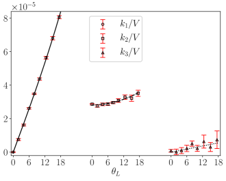
In Tab. 3 we summarize the results obtained for the topological observables $\chi$ and $b_{2}$ at different values of $N$ and of the lattice spacing, obtained by fitting the $\theta$ dependence of the cumulants as described in Sec. 2.2. An example of imaginary-$\theta$ fit of the cumulants is shown in Fig. 5 for the case $N=6$ and $\beta=25.75$.

In all the cases we found sufficient to fit the first three cumulants, as the addition of the fourth one did not change the obtained results. Moreover, in all cases we found the $O\left(\theta_{L}^{6}\right)$ term in the expansion of the vacuum energy to be well compatible with zero since no signal above zero is observed for $b_{4}$. In particular, we find $|b_{4}(N=4)|\cdot 10^{5}\lesssim 15$ and $|b_{4}(N=6)|\cdot 10^{5}\lesssim 30$. For this reason, results for $a^{4}\chi$ and $b_{2}$ reported in Tab. 3 have been obtained by neglecting $b_{4}$ in Eqs. (12). Finally we note that correlations between the different cumulants are small and do not significantly affect the result of the fit, as we explicitly checked by performing both correlated and uncorrelated fits.

$N=4$
$\beta$	$a\sqrt{\sigma}$	$Z$	$a^{4}\chi\cdot 10^{5}$	$b_{2}\cdot 10^{4}$
11.104	0.1981(5)	0.14742(96)	4.183(28)	-137.0(7.5)
11.347	0.1590(6)	0.1747(23)	1.691(22)	-128(11)
$N=6$
$\beta$	$a\sqrt{\sigma}$	$Z$	$a^{4}\chi\cdot 10^{5}$	$b_{2}\cdot 10^{4}$
24.768	0.2912(11)	0.10300(52)	18.371(93)	-77.2(8.3)
24.845	0.2801(13)	0.10945(68)	15.205(94)	-73.6(9.1)
25.056	0.2499(10)	0.12053(88)	9.719(69)	-72.9(8.6)
25.394	0.2143(8)	0.1382(12)	5.120(44)	-65.1(7.6)
25.750	0.1878(13)	0.1518(15)	2.816(27)	-58.7(7.4)

Table 3: Summary of the results obtained using the imaginary-$\theta$ fit for $N=4$ and $6$ by considering up to $O(\theta_{L}^{4})$ terms in the Taylor expansion of the vacuum energy, i.e., neglecting $b_{4}$ in Eqs. (12).

Figure 5: Best fit of the first 3 cumulants (solid, dashed and dotted line respectively) for $N=6$, $\beta=25.750$ and $\theta_{L}\in\left[0,17.5\right]$, obtained considering up to $O(\theta_{L}^{4})$ terms in the Taylor expansion of the vacuum energy, i.e., neglecting $b_{4}$ in Eqs. (12). The best fit yields $\chi^{2}/\mathrm{dof}=14.4/24$.

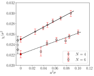
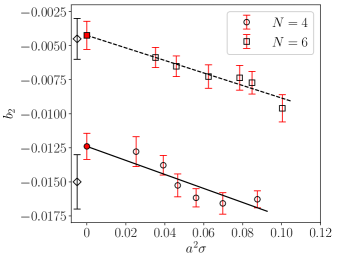
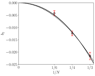
We used our data for $N=4$ and $N=6$, as well as data obtained for larger lattice spacings taken from Ref. Bonati et al. (2016a), to extrapolate continuum results for $\chi/\sigma^{2}$ and $b_{2}$. For the topological susceptibility the improvement with respect to previously available results is only marginal, since the dominant source of error comes from the string tension $\sigma$ used to set the scale. For $b_{2}$, instead, we achieved a substantial improvement of the state of the art, both for $N=4$ and $N=6$. In particular for $N=6$ parallel tempering allowed us to reach much finer lattice spacings than the ones used in previous studies. In this way we could perform for the first time a controlled continuum extrapolation of $b_{2}$ in this case, while in Ref. Bonati et al. (2016a) only a reasonable confidence interval was reported. In Tab. 4 we summarize our continuum limits, while in Fig. 6 we report our continuum extrapolations.

$N$	$\chi/\sigma^{2}$	$b_{2}$
3	0.0289(13)	-0.0216(15)
4	0.02499(54)	-0.01240(96)
6	0.02214(69)	-0.0042(10)

Table 4: Summary of continuum extrapolations for $N=3,4$ and $6$. Values for $N=3$ are taken from Ref. Bonati et al. (2016b).

Figure 6: Continuum extrapolations of $\chi/\sigma^{2}$ (above) and $b_{2}$ (below) for $N=4$ and $6$ (solid and dashed line respectively) obtained fitting linear corrections in $a^{2}\sigma$ to the continuum limit. The reported best fits yield, respectively for $N=4$ and $6$, $\chi^{2}/\rm{dof}=0.8/4$ and $3.7/4$ for $\chi/\sigma^{2}$ and $\chi^{2}/\rm{dof}=4.9/4$ and $1.2/4$ for $b_{2}$. The diamond points represent the determinations reported in Ref. Bonati et al. (2016a) for $N=4$ and 6.

3.3 Large-$N$ limit

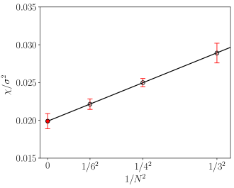
In this section we revisit the large-$N$ extrapolation on the basis of our improved results in particular we report our estimates of $\bar{\chi}$ and $\bar{b}_{2}$ introduced in Eq. (4). Let us start from the topological susceptibility: following large-$N$ expectations, we fitted our data for $N\geq 3$ using the functional form:

$$\frac{\chi}{\sigma^{2}}=\frac{\bar{\chi}}{\sigma^{2}}+\frac{k}{N^{2}}+O\left(\frac{1}{N^{4}}\right).$$ (18)

Our data are in agreement with the expected large-$N$ scaling and we find the result $\bar{\chi}/\sigma^{2}=0.0199(10)$; the best fit is shown in Fig. 7 together with numerical results. As already observed, our result does not improve the previous determination $\bar{\chi}/\sigma^{2}=0.0209(11)$ of Ref. Bonati et al. (2016a) as the main source of errors comes from the string tension used to set the scale. Using $\Lambda_{\mathit{large-}N}/\sqrt{\sigma}=0.525(2)$ Gonzalez-Arroyo and Okawa (2012) and $\Lambda_{\mathit{large-}N}=242(10)$ MeV Göckeler et al. (2005) to convert to physical units we get $\bar{\chi}^{1/4}=173(8)$ MeV, in agreement with the prediction $\bar{\chi}^{1/4}\simeq 180$ MeV obtained from the Witten–Veneziano formula.

Figure 7: Extrapolation of $\chi/\sigma^{2}$ towards the large-$N$ limit using fit function $\chi/\sigma^{2}=\bar{\chi}/\sigma^{2}+k/N^{2}$. Best fit yields $\bar{\chi}/\bar{\sigma}^{2}=0.0199(10)$ and $k=0.082(17)$.

We now pass to the discussion of the large-$N$ behavior of $b_{2}$. According to the standard large-$N$ arguments, we expect a behavior of the type:

$$b_{2}=\frac{\bar{b}_{2}}{N^{2}}+\frac{\bar{b}_{2}^{\left(1\right)}}{N^{4}}+O\left(\frac{1}{N^{6}}\right)\ .$$ (19)

To test this prediction we perform a best fit of our data with $N\geq 3$ using the power law $b_{2}(N)=\bar{b}_{2}/N^{c}$, obtaining a perfect agreement with expectations, since the exponent results $c=2.17(26)$, which improves the previous result $c=2.0(4)$ reported in Ref. Bonati et al. (2016a). The obtained best fit is shown in Fig. 8. By fixing the exponent $c=2$ and fitting our data with just the leading behavior $b_{2}=\bar{b}_{2}/N^{2}$ in the ranges $N\geq 3$ and $N\geq 4$, we obtain the results $\bar{b}_{2}=-0.1931(98)$ and $\bar{b}_{2}=-0.192(14)$ respectively. Since the curve profiles obtained in these two cases are practically indistinguishable, we only show the former in Fig. 8. As our final result, we quote the value $\bar{b}_{2}=-0.193(10)$, which improves on the previous determination $\bar{b}_{2}=-0.23(3)$ of Ref. Bonati et al. (2016a).

Figure 8: Extrapolation of $b_{2}$ towards the large-$N$ limit. The solid line represents the best fit obtained using fit function $b_{2}=\bar{b}_{2}/N^{c}$ in the whole range; the dashed line represents the best fit obtained using the same fit function but with fixed $c=2$ in the whole range; the dotted line represents the best fit obtained in the whole range including a further $\bar{b}_{2}^{\left(1\right)}/N^{4}$ term in the fit function. The best fits yield, respectively, $\bar{b}_{2}=-0.238(79),-0.1931(98)$ and $-0.179(31)$. The free exponent results $c=2.17(26)$, while the next-to-leading correction is $\bar{b}_{2}^{\left(1\right)}=-0.17(35)$.

4 Conclusions

In this work we investigated the $\theta$-dependence of $SU(N)$ Yang–Mills theories at zero temperature using the parallel tempering algorithm proposed by Hasenbusch in Ref. Hasenbusch (2017). This algorithm was originally tested in two dimensional $CP^{N-1}$ models, and a first extension of the original proposal has already been performed in Ref. Berni et al. (2019) (still for $CP^{N-1}$ models), by extending the parallel tempering approach to simulations at imaginary $\theta$ values. In the present work we implemented the same setup in $SU(N)$ Yang–Mills theory, thus proving the feasibility of the approach also for computationally more demanding models, and improving the state of the art results for the $\theta$ dependence of these models in the large $N$ limit.

The idea of the method is to simulate many independent identical systems differing only for the boundary conditions imposed on a cubic defect $L_{d}\times L_{d}\times L_{d}$, which are chosen to interpolate between open (obc) and periodic boundary conditions (pbc). Each replica evolves independently, and swaps among them are proposed from time to time in order to transfer configurations from the obc to the pbc replica. In this way a drastic reduction of the autocorrelation time of the topological charge is achieved, while avoiding the complication related to the breaking of translation invariance connected to the adoption of open boundary conditions, since measures are performed on the pbc replica.

By using the parallel tempering algorithm we got an impressive reduction of the autocorrelation times of topological observables, which for the smallest lattice spacing used was of at least two order of magnitude when taking into account also the larger computational complexity. A nice feature of the algorithm is that this gain was obtained without optimally tuning all the possible parameters entering the update, which proves the robustness of the approach. The most relevant parameter to be fixed is clearly the size of the defect, and we verified that for the cases studied in this paper a size in the range $0.2$–$0.3$ fm is sufficiently close to optimal to obtain a huge reduction of the critical slowing down.

The possibility of performing simulations at smaller lattice spacing than in previous studies allowed us to achieve a substantial improvement in the determination of $\theta$-dependence beyond the leading $O(\theta^{2})$ order. In particular, we improved the accuracy of the determination of the coefficients $b_{2}$ for both $N=4$ and $N=6$, in the last case also performing a controlled continuum limit extrapolation, which was not possible with previously available results. These data confirm that $b_{2}$ scales with the number of colors in a way that is consistent with the leading behavior predicted by large-$N$ arguments: data for $N\geq 3$ are perfectly compatible with a scaling of the form $b_{2}=\bar{b}_{2}/N^{2}$, with $\bar{b}_{2}=-0.193(10)$, while a best fit according to $b_{2}=\bar{b}_{2}/N^{c}$ returns the value $c=2.17(26)$ for the free exponent. This shows that the scaling of our data is consistent with the leading expected behavior, and it is thus reasonable to neglect sub-leading corrections. We however explicitly note that the accuracy is still not high enough to exclude possible unconventional scenarios like the one put-forward in Ref. Vonk et al. (2019), or to better investigate if critical corrections emerge at small $N$ Kitano et al. (2020).

A further refinement of present results, including also new values of $N$, would thus be welcome in the future: the algorithm proposed in Ref. Hasenbusch (2017), and extended to $SU(N)$ gauge theories in this study, will permit such systematic refinement.