Quantum walk on a ladder

Abstract

We study quantum walk on a ladder with combination of conventional and split-step protocols. The two components of the walk resulting from periodic boundary conditions can be made to have three kinds of probability distributions. Two of these are the one-sided and alternative ones. Using the differences between coin states of the individual component, we can simulate the third case in which both components have identical probability profiles. We also observe that the mutual information transfer between two components of the walk is minimized when this difference across the two sides of the ladder is maximized.

I Introduction

The term quantum walk (QW) was first introduced in the seminal work by Aharonov et al [1]. Since then, QWs have been studied from computation point of view such as in decision trees [2, 3], cellular automata [4], quantum search algorithms [5, 6, 7] and universal quantum computing [8, 9]. In addition, QWs have been used as a tool to explore topological phases [10, 11, 12, 13, 14, 15], photosynthetic energy transfer [16], Anderson localization and decoherence [17, 18, 19]. Several experiments with ions, atoms and photons [20, 21, 22, 23] have also been performed to realize QWs and to simulate its impressions on these phenomena [24, 25].

In continuous time quantum walk (CTQW), a quantum state is evolved by unitary operator $U\left(t\right)={\rm exp}\left(-iHt\right)$ for some time $T$ [26], with the Hamiltonian $H$ governing the walk. This idea is inspired from classical Markov chains where the role of $H$ is played by the adjacency matrix of the underlying graph. Whereas, in discrete time quantum walk (DTQW) [4], a quantum coin is used to guide the walker along a graph. The size of the wave packet after $n$ steps is given by [27],

$$\left\langle\Delta x^{2}\right\rangle=n^{2}\left(1-\left|sin\left(\gamma/2\right)\right|\right)$$ (1)

with $\gamma$ as the coin angle. This suggests the ballistic nature of QW compared to classical one which is diffusive in nature as $\left\langle\Delta x^{2}\right\rangle=n$. Moreover, it was also shown that DTQWs are faster than CTQWs [28], for further details please see Ref. [29], an excellent review on the subject.

There is much work done on DTQWs on graphs [30] and 2D lattices [31]. In a single dimension, the probability profile for quantum walk spreads at each step along the line. In higher dimensions this distribution is further extended along all direction depending on the protocol used for the walk. In a recent article [31], authors did analysis for a quantum walker on a cylinder. They showed that the boundary conditions on the closed side of cylinder implies several one dimensional walks characterized by their coin angles. They used conventional walk protocol and marginal probability as a measure. This protocol when used for the case of ladder, keeps the walk on one side, see Sec. IIA. On the other hand, in [32] authors considered two walkers on a line where due to entanglement and relative phases between the states influence the walk. Here, we explore DTQW on a ladder where due to the boundary conditions the walk is split into effectively two one dimensional components. The simple geometry of ladder lets us observe and control the behavior of individual component as well as the overall walk. Using split-step protocol, we can give richer possibilities for the walk. We also used magnetization like parameters discussed in Ref. [33] and thermodynamic-like quantities associated with the walk as in Ref. [34, 35, 36].

This article is organized as follows. In Sec. II, we describe the setup for our model. In particular, we will show that our choice of the split-step protocol provides more freedom for the walker. In Sec. III, we present our observation on the basis of few simple parameter in analogy with paramagnetism. We finally conclude and summarize in the last section.

II The choice of protocol

The state of a quantum walker is typically labeled by its position $\left|m\right\rangle$ and spin $\left|s\right\rangle$, degrees of freedom. Initially this state $\left|s,m\right\rangle=\left|s\right\rangle\otimes\left|m\right\rangle$ can be set to any position (usually taken to be localized) and spin (up, down or any mixture). Of course, these choices have effects on the final probability distribution. The state is then evolved through a given protocol for $N$ steps and the final state is projected over all positions to get the probability distribution for the walker [29].

The conventional protocol for 1DQW is the flip of coin followed by the shift operator as $\hat{U}^{{\rm con}}=\hat{T}\hat{C}\left(\gamma/2\right)$. Here $\hat{C}$ is the coin operator with some angle $\gamma\in\left[0,\pi\right]$. The general rotation of the coin allows for richer scenarios by changing the mixing between up and down components and hence more control over the walker. In this article we will use the coin introduced in the experiments as in Refs. [10, 11] and for exploring topological states [12],

$$\hat{C}\left(\gamma/2\right)=c\left|\uparrow\right\rangle\left\langle\uparrow\right|-s\left|\uparrow\right\rangle\left\langle\downarrow\right|+s\left|\downarrow\right\rangle\left\langle\uparrow\right|+c\left|\downarrow\right\rangle\left\langle\downarrow\right|,$$ (2)

where $c=cos\left(\gamma/2\right),s=sin\left(\gamma/2\right)$. The translation operator $\hat{T}$ decides the step direction by measuring the spin of the walker,

$$\hat{T}=\sum_{m=-\infty}^{\infty}\left(\left|\uparrow\right\rangle\left\langle\uparrow\right|\otimes\left|m+1\right\rangle\left\langle m\right|+\left|\downarrow\right\rangle\left\langle\downarrow\right|\otimes\left|m-1\right\rangle\left\langle m\right|\right).$$ (3)

Another choice for the walker on a line is to split the walk in two half-steps with use of two coins. The unitary evolution for split-step walk is $\hat{U}^{{\rm split}}=\hat{T}^{\downarrow}\hat{C}\left(\beta\right)\hat{T}^{\uparrow}\hat{C}\left(\alpha\right)$ where one component of the spin is moved and other is held after the flip of first coin. Then the next coin is flipped and the process is repeated for the other component. The half-shift operators are,

$$T^{\uparrow} = \sum_{m=-\infty}^{\infty}\left(\left|\uparrow\right\rangle\left\langle\uparrow\right|\otimes\left|m+1\right\rangle\left\langle m\right|+\left|\downarrow\right\rangle\left\langle\downarrow\right|\otimes\left|m\right\rangle\left\langle m\right|\right),$$ (4)

$$T^{\downarrow} = \sum_{m=-\infty}^{\infty}\left(\left|\uparrow\right\rangle\left\langle\uparrow\right|\otimes\left|m\right\rangle\left\langle m\right|+\left|\downarrow\right\rangle\left\langle\downarrow\right|\otimes\left|m-1\right\rangle\left\langle m\right|\right).$$ (5)

The one dimensional protocol can be extended to two dimensional quantum walks (2DQWs) with the coin operators replaced by the Groover coin or the product of Hadamard coins.

This article uses one of the result given in the work by Bru et al [31], where they discussed the 2DQW on a cylinder and showed that the boundary conditions implies a collection of 1DQWs with various group velocities. In Fig. 1, it is shown that the use of conventional protocol for both directions keeps the walker on one side of the ladder as in alternative quantum walk (AQW).

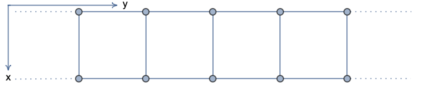
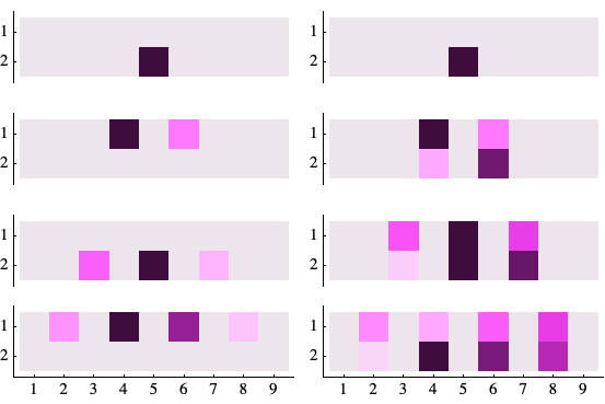
Figure 1:

First three step of the conventional (left) and split-step walk (right) on a ladder. For conventional walk, the longer side coin is set to $-\pi/4$ while for the shorter side it is $-\pi/8$. For split-step $\alpha=-\pi/4$ and $\beta=-\pi/2$.

Our aim is to keep the walker on both sides of the ladder. In figure 1, we show a simple ladder graph that is placed with its longer side along $y$ axis and shorter side along $x$ axis. For the longer side of the ladder, we choose the conventional protocol as $\hat{U}_{y}=\hat{T}\hat{C}\left(-\pi/4\right)$ with equal mixture of up and down spin components. However, if we use the split walk then the walker can be kept on both sides of the ladder. One step unitary evolution on the ladder can then be,

$$\hat{U}=\hat{U}_{y}^{{\rm split}}\hat{U}_{x}^{{\rm con}}=\hat{T}_{y}\hat{C}\left(\pi/4\right)\hat{T}_{x}^{\downarrow}\hat{C}\left(\beta/2\right)\hat{T}_{x}^{\uparrow}\hat{C}\left(\alpha/2\right).$$ (6)

We now impose the boundary conditions on the shorter side of the ladder. This leads to the quasi-momentum quantization along $x$ direction as $k_{x}=n\pi$. The translation operator takes two distinct values $+1$ or $-1$ as $e^{\pm ik_{x}}=\left(-1\right)^{n}$. This represents two one dimensional walkers moving along $y$ direction. The unitary operators for the two walkers are now,

$$\hat{U_{1}} = \hat{T}\left(k\right)\hat{C}\left(\gamma_{1}/2\right),$$ (7)

$$\hat{U_{2}} = \hat{T}\left(k\right)\hat{C}\left(\gamma_{2}/2\right),$$ (8)

where $\gamma_{1}=\alpha+\beta-\pi/2$ and $\gamma_{2}=\gamma_{1}+\phi=\alpha-\beta+3\pi/2$. Note that the phase difference between the coins is $\phi=\pm\left(2\beta-2\pi\right)$.

III Walk on the ladder

A variety of probability distributions can be produced by setting the coin angle to different values [37]. The dependance of walk on coin angle has analogy with paramagnet in a magnetic field [33], where the role of the magnetic field is replaced by the Bloch vector. As the angle of the coin is varied, the probability of up and down spin components is changed, as shown in Fig. 2. It can be seen from Eqs. (18) that the difference of these probabilities is $1-\left|sin\left(\gamma/2\right)\right|$ for one dimensional walk. This parameter gives hint about the walker’s distribution in position space [33].

In Fig. 2, the initial state is set at the center of the ladder on one side while the spin is set in up state. The angle of coin is then chosen as $0,\pi/4,\pi/2$ and $\pi$. At $\gamma=0$ and $\pi$, this parameter takes its maximum and minimum values respectively and the walk is classical-like. In former case, the walker moves without any spread while for the latter it just oscillates around its initial position. For the Hadamard, case the situation is like a fair classical coin. The probabilities for both up and down components are equal and hence the distribution is well spread over all points.

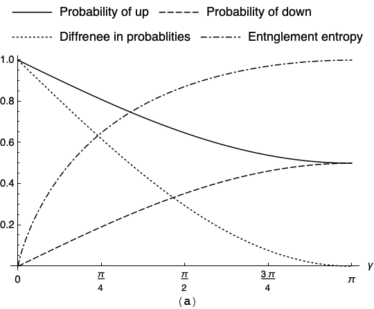
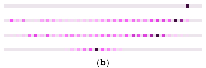
Figure 2:

a) Entropy and probabilities for a single walker with initial coin state $\left(1,0\right)^{T}$. b) One dimensional walk for 31 steps for coin angles $0,\pi/4,\pi/2$ and $\pi$ from top to bottom respectively (darker colors indicate higher probabilities).

We will now explore various walks on a ladder on the basis of these parameters. Since the walk is decomposed effectively into two one dimensional components, we can associate three such parameters. The first two are the usual ones for each side and can be written down immediately from Eqs. (18) as,

$$M_{1} = 1-\left|sin\left(\gamma_{1}/2\right)\right|,$$ (9)

$$M_{2} = 1-\left|sin\left(\gamma_{2}/2\right)\right|.$$ (10)

For the probability differences across the ladder, we define a third quantity as,

$$M = 1-\frac{1}{2}\left|sin\left(\frac{\gamma_{1}}{2}\right)\right|-\frac{1}{2}\left|sin\frac{1}{2}\left(\frac{\gamma_{2}}{2}\right)\right|.$$ (11)

$$= \frac{1}{2}\left(M_{1}+M_{2}\right)$$

This turns out to be merely the average of $M_{1}$ and $M_{2}$. Of course, this is also the difference between the diagonal components of full density matrix.

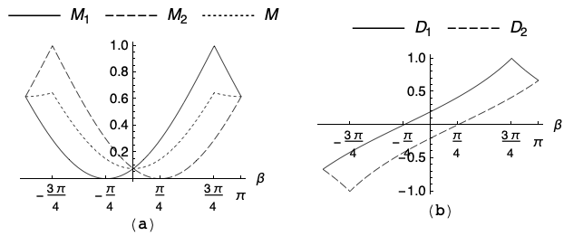
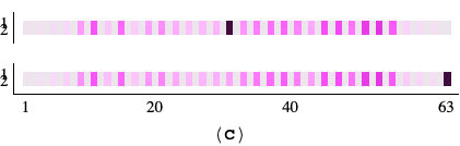
Figure 3:

a) $M_{1},M_{2}$ and $M$ vs $\beta$ for $\alpha=-\pi/4$. b) Discriminant of the eigenvalues of density matrices for two components. c) Identical walk for $\alpha=-\pi/4$ and $\beta=\pi/4,3\pi/4$.

For any value of $\alpha$, when $\beta$ is an odd multiple of $\pm\pi$, the walker is restricted to only one side of the ladder. It is also evident from the periodicity of Eqs. (9) and (10) that all three parameters are equal at these points. However, at $\beta=0$, the second coin is identity and the split-step walk is reduced to alternative walk between two sides of the ladder, see Fig. 1. As $\beta$ is changed from $\pm\pi$, the walk starts to split on both sides of the ladder until either $M_{1}$ or $M_{2}$ vanishes ($\alpha\pm\beta=-\pi/2$) or gets maximized ($\alpha\pm\beta=\pi/2$). At these points, the distribution on both sides of the ladder is identical as shown in Fig 3. The whole walk is dominated by one component as the second one is classical-like. These two cases are similar to 1DQW with coin angles $0$ and $\pi$, as in Fig. 2, except that the walkers are spread over all points. For the Hadamard cases when $\alpha=\pm\pi/2$, such cases can not be observed as the difference between $M_{1}$ and $M_{2}$ is zero for all values of $\beta$ and none of the components takes over. A summary of these results in given in Tab. 1.

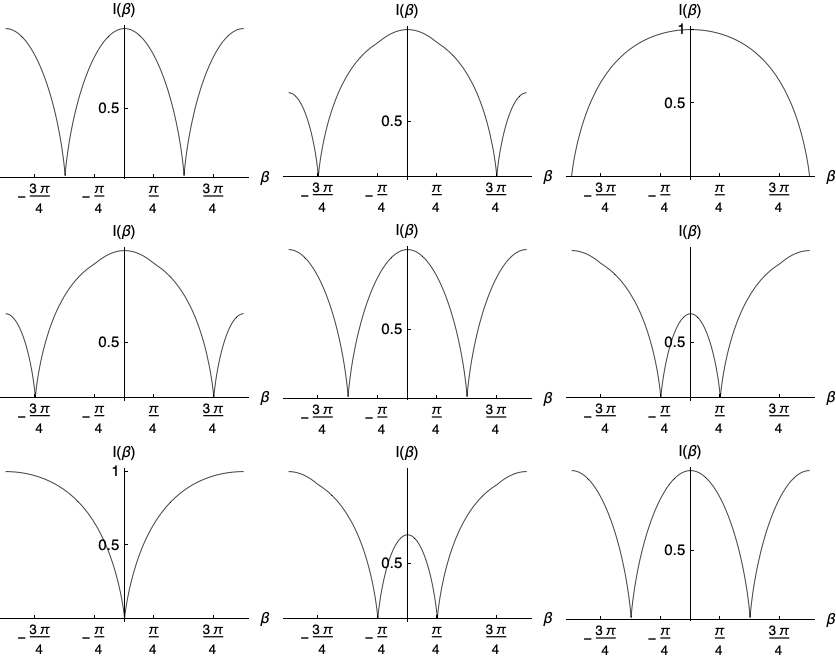
Figure 4: Mutual information $I$ vs $\beta$ for $\alpha\in\left[-\pi,\pi\right]$ in $\pi/4$ intervals.

Table 1: Summary of various walk pattern.

$\alpha\pm\beta$	Magnetization	Walk patterns
$\alpha\pm 0$	$M_{1}=M_{2}=M$	Alternating
$\alpha\pm\pi$	$M_{1}=M_{2}=M$	One-sided
$-\pi/2$	$M_{1}$or $M_{2}=0$	Identical
$\pi/2$	$M_{1}$or $M_{2}$ is maximized	Identical

We would like to remark that these arguments can be based on other quantities. For example, the discriminants in the eigenvalues of density matrices are of the form,

$$D=\frac{\left|cos\left(\gamma/4\right)\right|-\left|sin\left(\gamma/4\right)\right|}{\left|cos\left(\gamma/4\right)\right|+\left|sin\left(\gamma/4\right)\right|}.$$ (12)

In Fig 3. we have plotted $D_{1}$ and $D_{2}$ for both components where one can note the above mention cases. Indeed, various thermodynamic-like properties can be assigned to a quantum walker, which are related to these variables [34, 35, 36].

We finally use mutual quantum information [38] for the two components,

$$I=S\left(\rho_{1}\right)+S\left(\rho_{2}\right)-S\left(\rho\right),$$ (13)

to distinguish these two types identical distributions. Here $S\left(\rho_{1}\right)$, $S\left(\rho_{2}\right)$ and $S\left(\rho\right)$ are the von Neumann entropies associated with each component and overall walk, respectively. The zeros of this expression indicate the angles at which the two components are independent. As an example, $\alpha=-\pi/4$ and $\beta=\pm 3\pi/4$ corresponds to two independent walks while at $\beta=0$, both distributions are fully dependent on each other, see Fig 3 and Fig. 4. This may be the case as the walk is alternative at this value and hence each component is fully determined by the other.

IV Conclusion

We considered the simple situation for a quantum walker moving on a ladder. Using a specific mixed protocol for the walk, in contrast to conventional protocols, gives an extra option for the walker to be on both siders of the ladder. The analysis is done on the basis of probability differences of up and down spin components. We have also shown that for particular choices of two angles, the components can have almost similar probability profiles. As the walk evolves from one side of the ladder to the other, the mutual information is transferred from one component to the other. We have shown that this transfer is zero when the probability difference between up and down spin components across the ladder is maximum. These cases are simpler for a ladder but generalizing to a cylinder will need more angles and hence may not be feasible.

Appendix A Density matrices for the walk

The density matrix encodes the information about final state probabilities and hence the entropies for the quantum walk [39, 40, 32, 41, 42, 43, 38]. The evolutions of the two walkers can then be related to their corresponding density matrices. Since both walks are effectively one dimensional and differs only by coin angle, we will compute the density matrix for one walker and replace the coin angle for the other. For simplicity we choose the initial state of the walkers to be $\left|\psi\right\rangle_{0}=\left(1,0\right)^{T}$which corresponds to $\theta=0$ and $\phi=0$ on the Bloch sphere. The results can be easily generalized for a general state [44, 45].

The state $\left|\psi\right\rangle_{0}$ is then evolved $n$ times by the corresponding unitary operator which can be written using spectral decomposition as,

$$U^{n}=e^{-i\omega n}\left|e^{+}\right\rangle\left\langle e^{+}\right|+e^{i\omega n}\left|e^{-}\right\rangle\left\langle e^{-}\right|,$$ (14)

where $cos\omega_{\pm}=cos\left(\gamma/2\right)cosk$ is related to the eigenvalues $\lambda^{\pm}=e^{\pm i\omega}$of the unitary operator. The eigenvectors $\left|e^{\pm}\right\rangle$ of the unitary operator are given by,

$$\left|e^{\pm}\right\rangle=\frac{1}{N_{\pm}}\left(\begin{array}[]{c}u\\ -v^{\pm}+w\end{array}\right),$$ (15)

with,

$$u = e^{ik},$$

$$v = e^{ik}cot\left(\gamma/2\right),$$

$$w = cosec\left(\gamma/2\right)e^{\pm i\omega},$$ (16)

and normalization,

$$N^{\pm}=\frac{sin\left(\gamma/2\right)}{\sqrt{2\left[sin^{2}\omega\mp cos\left(\gamma/2\right)sinksin\omega\right]}}.$$ (17)

The evolved state $\left|\psi\right\rangle=\left(a\left(k\right),b\left(k\right)\right)^{T}$ is then used to compute the density matrix. In the large $n$ limit, it has the following elements,

$$\rho^{11} = 1-\frac{1}{2}\left|sin\left(\gamma/2\right)\right|,$$

$$\rho^{22} = 1-\rho^{11},$$

$$\rho^{12} = \rho^{21}=-\frac{1}{2}\left[1-sin\left(\gamma/2\right)\right]tan\left(\gamma/2\right).$$ (18)

Here we used the fact that ${\rm tr}\left(\rho\right)=1$, as a consequence of probability conservation.

With definition, $\Delta=\text{$\rho^{11}\rho^{22}$}-\left|\rho^{12}\right|^{2}$ the eigenvalues of the density matrix can be computed as,

$$\Lambda^{\pm} = \frac{1}{2}\left(1\pm\sqrt{1-4\Delta}\right)$$ (19)

$$= \frac{1}{1+tan\left(\gamma/2\right)},\frac{1}{1+cot\left(\gamma/2\right)}$$

For each component we can now replace $\gamma$ by $\gamma_{1}$ and $\gamma_{2}$. The full density matrix is then the average of these density matrices. Finally the entanglement entropies can be computed using,

$$S=-\Lambda^{-}{\rm log}_{2}\Lambda^{-}-\Lambda^{+}{\rm log}_{2}\Lambda^{+},$$ (20)

for each component and the whole walk.

References

- Aharonov et al. [1993] Y. Aharonov, L. Davidovich, and N. Zagury, Quantum random walks, Phys. Rev. A 48, 1687 (1993).
- Farhi and Gutmann [1992] E. Farhi and S. Gutmann, The functional integral constructed directly from the hamiltonian, Annals of Physics 213, 182 (1992).
- Farhi and Gutmann [1998] E. Farhi and S. Gutmann, Quantum computation and decision trees, Phys. Rev. A 58, 915 (1998).
- Meyer [1996] D. A. Meyer, From quantum cellular automata to quantum lattice gases, Journal of Statistical Physics 85, 551 (1996).
- Shenvi et al. [2003] N. Shenvi, J. Kempe, and K. B. Whaley, Quantum random-walk search algorithm, Phys. Rev. A 67, 052307 (2003).
- Ambainis [2004] A. Ambainis, Quantum search algorithms, ACM SIGACT News 35, 22 (2004).
- Kendon [2006] V. M. Kendon, A random walk approach to quantum algorithms, Philosophical Transactions of the Royal Society A: Mathematical, Physical and Engineering Sciences 364, 3407 (2006).
- Childs [2009] A. M. Childs, Universal computation by quantum walk, Phys. Rev. Lett. 102, 180501 (2009).
- Lovett et al. [2010] N. B. Lovett, S. Cooper, M. Everitt, M. Trevers, and V. Kendon, Universal quantum computation using the discrete-time quantum walk, Phys. Rev. A 81, 042330 (2010).
- Karski et al. [2009] M. Karski, L. Förster, J.-M. Choi, A. Steffen, W. Alt, D. Meschede, and A. Widera, Quantum walk in position space with single optically trapped atoms, Science 325, 174 (2009).
- Zähringer et al. [2010] F. Zähringer, G. Kirchmair, R. Gerritsma, E. Solano, R. Blatt, and C. F. Roos, Realization of a quantum walk with one and two trapped ions, Phys. Rev. Lett. 104, 100503 (2010).
- Kitagawa et al. [2010] T. Kitagawa, M. S. Rudner, E. Berg, and E. Demler, Exploring topological phases with quantum walks, Phys. Rev. A 82, 033429 (2010).
- Zhan et al. [2017] X. Zhan, L. Xiao, Z. Bian, K. Wang, X. Qiu, B. C. Sanders, W. Yi, and P. Xue, Detecting topological invariants in nonunitary discrete-time quantum walks, Phys. Rev. Lett. 119, 130501 (2017).
- Wang et al. [2018] B. Wang, T. Chen, and X. Zhang, Experimental observation of topologically protected bound states with vanishing chern numbers in a two-dimensional quantum walk, Phys. Rev. Lett. 121, 100501 (2018).
- Zhang et al. [2017] W.-W. Zhang, B. C. Sanders, S. Apers, S. K. Goyal, and D. L. Feder, Detecting topological transitions in two dimensions by hamiltonian evolution, Phys. Rev. Lett. 119, 197401 (2017).
- Mohseni et al. [2008] M. Mohseni, P. Rebentrost, S. Lloyd, and A. Aspuru-Guzik, Environment-assisted quantum walks in photosynthetic energy transfer, The Journal of Chemical Physics 129, 174106 (2008).
- Schreiber et al. [2011] A. Schreiber, K. N. Cassemiro, V. Potoček, A. Gábris, I. Jex, and C. Silberhorn, Decoherence and disorder in quantum walks: From ballistic spread to localization, Phys. Rev. Lett. 106, 180403 (2011).
- Crespi et al. [2013] A. Crespi, R. Osellame, R. Ramponi, V. Giovannetti, R. Fazio, L. Sansoni, F. D. Nicola, F. Sciarrino, and P. Mataloni, Anderson localization of entangled photons in an integrated quantum walk, Nature Photonics 7, 322 (2013).
- Edge and Asboth [2015] J. M. Edge and J. K. Asboth, Localization, delocalization, and topological transitions in disordered two-dimensional quantum walks, Phys. Rev. B 91, 104202 (2015).
- Schmitz et al. [2009] H. Schmitz, R. Matjeschk, C. Schneider, J. Glueckert, M. Enderlein, T. Huber, and T. Schaetz, Quantum walk of a trapped ion in phase space, Phys. Rev. Lett. 103, 090504 (2009).
- Broome et al. [2010] M. A. Broome, A. Fedrizzi, B. P. Lanyon, I. Kassal, A. Aspuru-Guzik, and A. G. White, Discrete single-photon quantum walks with tunable decoherence, Phys. Rev. Lett. 104, 153602 (2010).
- Schreiber et al. [2010] A. Schreiber, K. N. Cassemiro, V. Potoček, A. Gábris, P. J. Mosley, E. Andersson, I. Jex, and C. Silberhorn, Photons walking the line: A quantum walk with adjustable coin operations, Phys. Rev. Lett. 104, 050502 (2010).
- Alberti et al. [2014] A. Alberti, W. Alt, R. Werner, and D. Meschede, Decoherence models for discrete-time quantum walks and their application to neutral atom experiments, New Journal of Physics 16, 123052 (2014).
- Obuse and Kawakami [2011] H. Obuse and N. Kawakami, Topological phases and delocalization of quantum walks in random environments, Phys. Rev. B 84, 195139 (2011).
- Rakovszky and Asboth [2015] T. Rakovszky and J. K. Asboth, Localization, delocalization, and topological phase transitions in the one-dimensional split-step quantum walk, Phys. Rev. A 92, 052311 (2015).
- Childs et al. [2002] A. M. Childs, E. Farhi, and S. Gutmann, An example of the difference between quantum and classical random walks, Quantum Information Processing 1, 35 (2002).
- Ahlbrecht et al. [2011] A. Ahlbrecht, H. Vogts, A. H. Werner, and R. F. Werner, Asymptotic evolution of quantum walks with random coin, Journal of Mathematical Physics 52, 042201 (2011).
- Ambainis et al. [2005] A. Ambainis, J. Kempe, and A. Rivosh, Coins make quantum walks faster, in Proceedings of the Sixteenth Annual ACM-SIAM Symposium on Discrete Algorithms, SODA ’05 (Society for Industrial and Applied Mathematics, USA, 2005) pp. 1099–1108.
- Kempe [2003] J. Kempe, Quantum random walks: An introductory overview, Contemporary Physics 44, 307 (2003).
- Aharonov et al. [2001] D. Aharonov, A. Ambainis, J. Kempe, and U. Vazirani, Quantum walks on graphs, in Proceedings of the thirty-third annual ACM symposium on Theory of computing - STOC '01 (ACM Press, 2001).
- Bru et al. [2016] L. A. Bru, G. J. de Valcárcel, G. D. Molfetta, A. Pérez, E. Roldán, and F. Silva, Quantum walk on a cylinder, Phys. Rev. A 94, 032328 (2016).
- Omar et al. [2006] Y. Omar, N. Paunković, L. Sheridan, and S. Bose, Quantum walk on a line with two entangled particles, Phys. Rev. A 74, 042304 (2006).
- Souza and Andrade [2013] A. M. C. Souza and R. F. S. Andrade, Coin state properties in quantum walks, Scientific Reports 3, 10.1038/srep01976 (2013).
- Romanelli [2012] A. Romanelli, Thermodynamic behavior of the quantum walk, Phys. Rev. A 85, 012319 (2012).
- Romanelli [2015] A. Romanelli, Quantum walk, entanglement and thermodynamic laws, Physica A: Statistical Mechanics and its Applications 434, 111 (2015).
- Vallejo et al. [2019] A. Vallejo, A. Romanelli, R. Donangelo, and R. Portugal, Entropy production in the quantum walk, Phys. Rev. A 99, 032319 (2019).
- Panahiyan and Fritzsche [2018] S. Panahiyan and S. Fritzsche, Controlling quantum random walk with a step-dependent coin, New Journal of Physics 20, 083028 (2018).
- Xue and Sanders [2012] P. Xue and B. C. Sanders, Two quantum walkers sharing coins, Phys. Rev. A 85, 022307 (2012).
- Endrejat and Büttner [2005] J. Endrejat and H. Büttner, Entanglement measurement with discrete multiple-coin quantum walks, Journal of Physics A: Mathematical and General 38, 9289 (2005).
- Venegas-Andraca et al. [2005] S. E. Venegas-Andraca, J. L. Ball, K. Burnett, and S. Bose, Quantum walks with entangled coins, New Journal of Physics 7, 221 (2005).
- Pathak and Agarwal [2007] P. K. Pathak and G. S. Agarwal, Quantum random walk of two photons in separable and entangled states, Phys. Rev. A 75, 032351 (2007).
- Liu and Petulante [2009] C. Liu and N. Petulante, One-dimensional quantum random walks with two entangled coins, Phys. Rev. A 79, 032312 (2009).
- Annabestani et al. [2010] M. Annabestani, M. R. Abolhasani, and G. Abal, Asymptotic entanglement in 2d quantum walks, Journal of Physics A: Mathematical and Theoretical 43, 075301 (2010).
- Nayak and Vishwanath [2000] A. Nayak and A. Vishwanath, Quantum walk on the line, arxiv:quant-ph/0010117 (2000).
- Abal et al. [2006] G. Abal, R. S. A. Romanelli, and R. Donangelo, Quantum walk on the line: Entanglement and nonlocal initial conditions, Phys. Rev. A 73, 042302 (2006).