Explaining NLP Models via Minimal Contrastive Editing ()

Abstract

Humans have been shown to give contrastive explanations, which explain why an observed event happened rather than some other counterfactual event (the contrast case). Despite the influential role that contrastivity plays in how humans explain, this property is largely missing from current methods for explaining NLP models. We present Minimal Contrastive Editing (), a method for producing contrastive explanations of model predictions in the form of edits to inputs that change model outputs to the contrast case. Our experiments across three tasks—binary sentiment classification, topic classification, and multiple-choice question answering—show that is able to produce edits that are not only contrastive, but also minimal and fluent, consistent with human contrastive edits. We demonstrate how edits can be used for two use cases in NLP system development—debugging incorrect model outputs and uncovering dataset artifacts—and thereby illustrate that producing contrastive explanations is a promising research direction for model interpretability.

1 Introduction

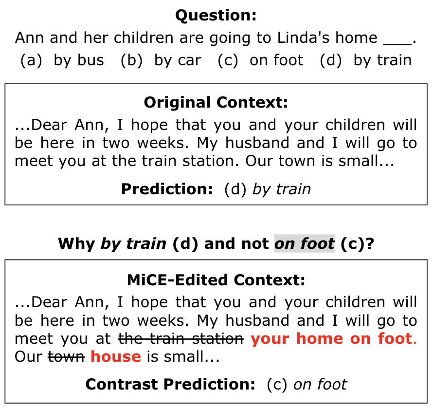
Figure 1: An example edit for a multiple-choice question from the Race dataset. generates contrastive explanations in the form of edits to inputs that change model predictions to target (contrast) predictions. The edit (bolded in red) is minimal and fluent, and it changes the model’s prediction from “by train” to the contrast prediction “on foot” (highlighted in gray).

Cognitive science and philosophy research has shown that human explanations are contrastive (Miller, 2019): People explain why an observed event happened rather than some counterfactual event called the contrast case. This contrast case plays a key role in modulating what explanations are given. Consider Figure 1. When we seek an explanation of the model’s prediction “by train,” we seek it not in absolute terms, but in contrast to another possible prediction (i.e. “on foot”). Additionally, we tailor our explanation to this contrast case. For instance, we might explain why the prediction is “by train” and not “on foot” by saying that the writer discusses meeting Ann at the train station instead of at Ann’s home on foot; such information is captured by the edit (bolded red) that results in the new model prediction “on foot.” For a different contrast prediction, such as “by car,” we would provide a different explanation. In this work, we propose to give contrastive explanations of model predictions in the form of targeted minimal edits, as shown in Figure 1, that cause the model to change its original prediction to the contrast prediction.

Given the key role that contrastivity plays in human explanations, making model explanations contrastive could make them more user-centered and thus more useful for their intended purposes, such as debugging and exposing dataset biases Ribera and Lapedriza (2019)—purposes which require that humans work with explanations Alvarez-Melis et al. (2019). However, many currently popular instance-based explanation methods produce highlights—segments of input that support a prediction (Zaidan et al., 2007; Lei et al., 2016; Chang et al., 2019; Bastings et al., 2019; Yu et al., 2019; DeYoung et al., 2020; Jain et al., 2020; Belinkov and Glass, 2019) that can be derived through gradients (Simonyan et al., 2014; Smilkov et al., 2017; Sundararajan et al., 2017), approximations with simpler models (Ribeiro et al., 2016), or attention (Wiegreffe and Pinter, 2019; Sun and Marasović, 2021). These methods are not contrastive, as they leave the contrast case undetermined; they do not tell us what would have to be different for a model to have predicted a particular contrast label.

As an alternative approach to NLP model explanation, we introduce Minimal Contrastive Editing ()—a two-stage approach to generating contrastive explanations in the form of targeted minimal edits (as shown in Figure 1). Given an input, a fixed Predictor model, and a contrast prediction, generates edits to the input that change the Predictor’s output from the original prediction to the contrast prediction. We formally define our edits and describe our approach in §2.

We design to produce edits with properties motivated by human contrastive explanations. First, we desire edits to be minimal, altering only small portions of input, a property which has been argued to make explanations more intelligible (Alvarez-Melis et al., 2019; Miller, 2019). Second, edits should be fluent, resulting in text natural for the domain and ensuring that any changes in model predictions are not driven by inputs falling out of distribution of naturally occurring text. Our experiments (§3) on three English-language datasets, Imdb, Newsgroups, and Race, validate that edits are indeed contrastive, minimal, and fluent.

We also analyze the quality of edits (§4) and show how they may be used for two use cases in NLP system development. First, we show that edits are comparable in size and fluency to human edits on the Imdb dataset. Next, we illustrate how edits can facilitate debugging individual model predictions. Finally, we show how edits can be used to uncover dataset artifacts learned by a powerful Predictor model.

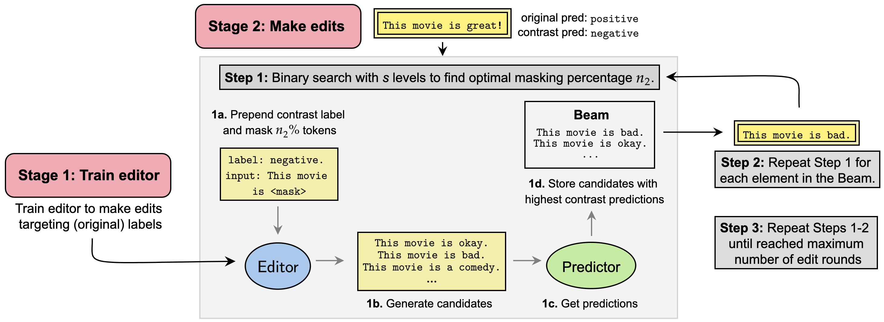
Figure 2: An overview of , our two-stage approach to generating edits. In Stage 1 (§2.3), we train the Editor to make edits targeting specific predictions from the Predictor. In Stage 2 (§2.4), we make contrastive edits with the Editor model from Stage 1 such that the Predictor changes its output to the contrast prediction.

2 : Minimal Contrastive Editing

This section describes our proposed method, Minimal Contrastive Editing, or , for explaining NLP models with contrastive edits.

2.1 Edits as Contrastive Explanations

Contrastive explanations are answers to questions of the form Why p and not q? They explain why the observed event $p$ happened instead of another event $q$, called the contrast case. A long line of research in the cognitive sciences and philosophy has found that human explanations are contrastive (Van Fraassen, 1980; Lipton, 1990; Miller, 2019). Human contrastive explanations have several hallmark characteristics. First, they cite contrastive features: features that result in the contrast case when they are changed in a particular way (Chin-Parker and Cantelon, 2017). Second, they are minimal in the sense that they rarely cite the entire causal chain of a particular event, but select just a few relevant causes (Hilton, 2017). In this work, we argue that a minimal edit to a model input that causes the model output to change to the contrast case has both these properties and can function as an effective contrastive explanation. We first give an illustration of contrastive explanations humans might give and then show how minimal contrastive edits offer analogous contrastive information.

As an example, suppose we want to explain why the answer to the question “Q: Where can you find a clean pillow case that is not in use?” is “A: the drawer.” If someone asks why the answer is not “C1: on the bed,” we might explain: “E1: Because only the drawer stores pillow cases that are not in use.” However, E1 would not be an explanation of why the answer is not “C2: in the laundry hamper,” since both drawers and laundry hampers store pillow cases that are not in use. For contrast case C2, we might instead explain: “E2: Because only laundry hampers store pillow cases that are not clean.” We cite different parts of the original question depending on the contrast case.

In this work, we propose to offer contrastive explanations in the form of minimal edits that result in the contrast case as model output. Such edits are effective contrastive explanations because, by construction, they highlight contrastive features. For example, a contrastive edit of the original question for contrast case C1 would be: “Where can you find a clean pillow case that is not in use?”; the information provided by this edit—that it is whether or not the pillow case is in use that determines whether the answer is “the drawer” or “on the bed”—is analogous to the information provided by E1. Similarly, a contrastive edit for contrast case C2 that changed the question to “Where can you find a clean dirty pillow case that is not in use?” provides analogous information to E2.

2.2 Overview of

We define a contrastive edit to be a modification of an input instance that causes a Predictor model (whose behavior is being explained) to change its output from its original prediction for the unedited input to a given target (contrast) prediction. Formally, for textual inputs, given a fixed Predictor $f$, input $\bm{x}=(x_{1},x_{2},...,x_{N})$ of $N$ tokens, original prediction $f(\bm{x})=y_{p}$ and contrast prediction $y_{c}\neq y_{p}$, a contrastive edit is a mapping $e:(x_{1},...,x_{N})\rightarrow(x_{1}^{\prime},...,x_{M}^{\prime})$ such that $f(e(\bm{x}))=y_{c}$.

We propose , a two-stage approach to generating contrastive edits, illustrated in Figure 2. In Stage 1, we prepare a highly-contextualized Editor model to associate edits with given end-task labels (i.e., labels for the task of the Predictor) such that the contrast label $y_{c}$ is not ignored in ’s second stage. Intuitively, we do this by masking the spans of text that are “important” for the given target label (as measured by the Predictor’s gradients) and training our Editor to reconstruct these spans of text given the masked text and target label as input. In Stage 2 of , we generate contrastive edits $e(\bm{x})$ using the Editor model from Stage 1. Specifically, we generate candidate edits $e(\bm{x})$ by masking different percentages of $\bm{x}$ and giving masked inputs with prepended contrast label $y_{c}$ to the Editor; we use binary search to find optimal masking percentages and beam search to keep track of candidate edits that result in the highest probability of the contrast labels $p(y_{c}|e(\bm{x}))$ given by the Predictor.

2.3 Stage 1: Fine-tuning the Editor

In Stage 1 of , we fine-tune the Editor to infill masked spans of text in a targeted manner. Specifically, we fine-tune a pretrained model to infill masked spans given masked text and a target end-task label as input. In this work, we use the Text-to-Text Transfer Transformer (T5) model (Raffel et al., 2020) as our pretrained Editor, but any model suitable for span infilling can in principle be the Editor in . The addition of the target label allows the highly-contextualized Editor to condition its predictions on both the masked context and the given target label such that the contrast label is not ignored in Stage 2. What to use as target labels during Stage 1 depends on who the end-users of are. The end-user could be: (1) a model developer who has access to the labeled data used to train the predictor, or (2) lay-users, domain experts, or other developers without access to the labeled data. In the former case, we could use the gold label as targets, and in the latter case, we could use the labels predicted by Predictor. Therefore, during fine-tuning, we experiment with using both gold labels and original predictions $y_{p}$ of our Predictor model as target labels. To provide target labels, we prepend them to inputs to the Editor. For more information about how these inputs are formatted, see Appendix B. Results in Table 2 show that fine-tuning with target labels results in better edits than fine-tuning without them.

The above procedure allows our Editor to condition its infilled spans on both the context and the target label. But this still leaves open the question of where to mask our text. Intuitively, we want to mask the tokens that contribute most to the Predictor’s predictions, since these are the tokens that are most strongly associated with the target label. We propose to use gradient attribution (Simonyan et al., 2014) to choose tokens to mask. For each instance, we take the gradient of the predicted logit for the target label with respect to the embedding layers of $f$ and take the $\ell_{1}$ norm across the embedding dimension. We then mask the $n_{1}\%$ of tokens with the highest gradient norms. We replace consecutive tokens (i.e., spans) with sentinel tokens, following Raffel et al. (2020). Results in Table 1 show that gradient-based masking outperforms random masking.

2.4 Stage 2: Making Edits with the Editor

In the second stage of our approach, we use our fine-tuned Editor to make edits using beam search Reddy (1977). In each round of edits, we mask consecutive spans of $n_{2}\%$ of tokens in the original input, prepend the contrast prediction to the masked input, and feed the resulting masked instance to the Editor; the Editor then generates $m$ edits. The masking procedure during this stage is gradient-based as in Stage 1.

In one round of edits, we conduct a binary search with $s$ levels over values of $n_{2}$ between values $n_{2}=0\%$ to $n_{2}=55\%$ to efficiently find a value of $n_{2}$ that is large enough to result in the contrast prediction while also modifying only minimal parts of the input. After each round of edits, we get $f$’s predictions on the edited inputs, order them by contrast prediction probabilities, and update the beam to store the top $b$ edited instances. As soon as an edit $e^{*}=e(\bm{t})$ is found that results in the contrast prediction, i.e., $f(e^{*})=y_{c}$, we stop the search procedure and return this edit. For generation, we use a combination of top-k (Fan et al., 2018) and top-p (nucleus) sampling (Holtzman et al., 2020).

Variant	Imdb			Newsgroups			Race
	$\uparrow$	$\downarrow$	$\approx 1$	$\uparrow$	$\downarrow$	$\approx 1$	$\uparrow$	$\downarrow$	$\approx 1$
	Flip Rate	Minim.	Fluen.	Flip Rate	Minim.	Fluen.	Flip Rate	Minim.	Fluen.
*Pred + Grad	$\mathbf{1.000}$	$\mathbf{0.173}$	$\mathbf{0.981}$	$\mathbf{0.992}$	$\mathbf{0.261}$	$0.968$	$0.915$	$\mathbf{0.331}$	$\mathbf{0.981}$
*Gold + Grad	$\mathbf{1.000}$	$0.185$	$0.979$	$\mathbf{0.992}$	${0.271}$	$0.966$	$\mathbf{0.945}$	$0.335$	$0.979$
Pred + Rand	$\mathbf{1.000}$	$0.257$	$0.958$	$0.968$	$0.378$	$0.928$	$0.799$	$0.440$	$0.953$
Gold + Rand	$\mathbf{1.000}$	$0.302$	$0.952$	$0.965$	$0.370$	$0.929$	$0.801$	$0.440$	$0.955$
No-Finetune	$0.995$	$0.360$	$0.960$	$0.941$	$0.418$	$0.938$	–	–	–

Table 1: Efficacy of the procedure. We evaluate edits on three metrics (described in §3.1): flip rate, minimality, and fluency. We report mean values for minimality and fluency. * marks full variants; others explore ablations. For each property (i.e., column), the best value across variants is bolded. We experiment with Predictor’s predictions (Pred) and gold labels (Gold) as target labels during Stage 1. Across datasets, our Grad procedure achieves a high flip rate with small and fluent edits.

3 Evaluation

This section presents empirical findings that produces minimal and fluent contrastive edits.

3.1 Experimental Setup

Tasks

We evaluate on three English-language datasets: IMDB, a binary sentiment classification task (Maas et al., 2011), a 6-class version of the 20 Newsgroups topic classification task (Lang, 1995), and Race, a multiple choice question-answering task (Lai et al., 2017).

Predictors

can be used to make contrastive edits for any differentiable Predictor model, i.e., any end-to-end neural model. In this paper, for each task, we train a Predictor model $f$ built on RoBERTa-large (Liu et al., 2019), and fix it during evaluation. The test accuracies of our Predictors are 95.9%, 85.3% and 84% for Imdb, Newsgroups, and Race, respectively. For training details, see Appendix A.1.

Editors

Our Editors build on the base version of T5. For fine-tuning our Editors (Stage 1), we use the original training data used to train Predictors. We randomly split the data, 75%/25% for fine-tuning/validation and fine-tune until the validation loss stops decreasing (for a max of 10 epochs) with $n_{1}\%$ of tokens masked, where $n_{1}$ is a randomly chosen value in $[20,55]$. For more details, see Appendix A.2. In Stage 2, for each instance, we set the label with the second highest predicted probability as the contrast prediction. We set beam width $b=3$, consider $s=4$ search levels during binary search over $n_{2}$ in each edit round, and run our search for a max of 3 edit rounds. For each $n_{2}$, we sample $m=15$ generations from our fine-tuned Editors with $p=0.95$, $k=30$.

Metrics

We evaluate on the test sets of the three datasets. The Race and Newsgroups test sets contain 4,934 and 7,307 instances, respectively. For Imdb, we randomly sample 5K of the 25K instances in the test set for evaluation because of the computational demands of evaluation.

For each dataset, we measure the following three properties: (1)  flip rate: the proportion of instances for which an edit results in the contrast label; (2)  minimality: the “size” of the edit as measured by the word-level Levenshtein distance between the original and edited input, which is the minimum number of deletions, insertions, or substitutions required to transform one into the other. We report a normalized version of this metric with a range from 0 to 1—the Levenshtein distance divided by the number of words in the original input; (3)   fluency: a measure of how similarly distributed the edited output is to the original data. We evaluate fluency by comparing masked language modeling loss on both the original and edited inputs using a pretrained model. Specifically, given the original $N$-length sequence, we create $N$ copies, each with a different token replaced by a mask token, following Salazar et al. (2020). We then take a pretrained t5-base model and compute the average loss across these $N$ copies. We compute this loss value for both the original input and edited input and report their ratio—i.e., edited $/$ original. We aim for a value of 1.0, which indicates equivalent losses for the original and edited texts. When finds multiple edits, we report metrics for the edit with the smallest value for minimality.

3.2 Results

Results are shown in Table 1. Our proposed Grad procedure (upper part of Table 1) achieves a high flip rate across all three tasks. This is the outcome regardless of whether predicted target labels (first row, 91.5–100% flip rate) or gold target labels (second row, 94.5–100% flip rate) are used for fine-tuning in Stage 1. We observe a slight improvement from using the gold labels for the Race Predictor, which may be explained by the fact that it is less accurate (with a training accuracy of $89.9\%$) than the Imdb and Newsgroups classifiers.

achieves a high flip-rate while its edits remain small and result in fluent text. In particular, on average changes 17.3–33.1% of the original tokens when predicted labels are used in Stage 1 and 18.5–33.5% with gold labels. Fluency is close to 1.0 indicating no notable change in mask language modeling loss after the edit—i.e., edits fall in distribution of the original data. We achieve the best results across metrics on the Imdb dataset, as expected since Imdb is a binary classification task with a small label space. These results demonstrate that presents a promising research direction for the generation of contrastive explanations; however, there is still room for improvement, especially for more challenging tasks such as Race.

In the rest of this section, we provide results from several ablation experiments.

Fine-tuning vs. No Fine-tuning

We investigate the effect of fine-tuning (Stage 1) with a baseline that skips Stage 1 altogether. For this No-Finetune baseline variant of , we use the vanilla pretrained T5-base as our Editor. As shown in Table 1, the No-Finetune variant underperforms all other (two-stage) variants of for the Imdb and Newsgroups datasets. Fine-tuning particularly improves the minimality of edits, while leaving the flip rate high. We hypothesize that this effect is due to the effectiveness of Stage 2 of at finding contrastive edits: Because we iteratively generate many candidate edits using beam search, we are likely to find a prediction-flipping edit. Fine-tuning allows us to find such an edit at a lower masking percentage.

Gradient vs. Random Masking

We study the impact of using gradient-based masking in Stage 1 of the procedure with a Rand variant, which masks spans of randomly chosen tokens. As shown in the middle part of Table 1, gradient-based masking outperforms random masking when using both predicted and gold labels across all three tasks and metrics, suggesting that the gradient-based attribution used to mask text during Stage 1 of is an important part of the procedure. The differences are especially notable for Race, which is the most challenging task according to our metrics.

Imdb Condition		$\uparrow$	$\downarrow$	$\approx 1$
Stage 1	Stage 2	Flip Rate	Minim.	Fluen.
No Label	No Label	$0.994$	$0.369$	$0.966$
No Label	Label	$0.997$	$0.362$	$0.967$
Label	No Label	$0.999$	$0.327$	$0.968$
Label	Label	$\mathbf{1.000}$	$\mathbf{0.173}$	$\mathbf{0.981}$

Table 2: Effect of using target end-task labels during the two stages of PRED+GRAD on the Imdb dataset. When end-task labels are provided, they are original Predictor labels during Stage 1 and contrast labels during Stage 2. The best values for each property (column) are bolded. Using end-task labels during both Stage 1 (Editor fine-tuning) and Stage 2 (making edits) of outperforms all other conditions.

Targeted vs. Un-targeted Infilling

We investigate the effect of using target labels in both stages of by experimenting with removing target labels during Stage 1 (Editor fine-tuning) and Stage 2 (making edits). As shown in Table 2, we observe that giving target labels to our Editors during both stages of improves edit quality. Fine-tuning Editors without labels in Stage 1 (“No Label”) leads to worse flip rate, minimality, and fluency than does fine-tuning Editors with labels (“Label”). Minimality is particularly affected, and we hypothesize that using target end-task labels in both stages provides signal that allows the Editor in Stage 2 to generate prediction-flipping edits at lower masking percentages.

Imdb	Original pred $y_{p}=$ positive       Contrast pred $y_{c}=$ negative An interesting pairing of stories, this little flick manages to bring together seemingly different characters and story lines all in the backdrop of WWII and succeeds in tying them together without losing the audience. I was impressed by the depth portrayed by the different characters and also by how much I really felt I understood them and their motivations, even though the time spent on the development of each character was very limited. The outstanding acting abilities of the individuals involved with this picture are easily noted. A fun, stylized movie with a slew of comic moments and a bunch more head shaking events. 7/10 4/10
Race	(a)  twice   (b)  only once  (c)  several times   (d)  once or twice.
	Original pred $y_{p}=(a)\,$ twice       Contrast pred $y_{c}=(b)\,$ only once When George was thirty-five, he bought a small plane and learned to fly it. He soon became very good and made his plane do all kinds of tricks. George had a friend, whose name was Mark. One day George offered to take Mark up in his plane. Mark thought, "I’ve traveled in a big plane several times, but I’ve never been in a small one, so I’ll go." They went up, and George flew around for half an hour and did all kinds of tricks in the air. When they came down again, Mark was glad to be back safely, and he said to his friend in a shaking voice, "Well, George, thank you very much for those two trips tricks in your plane." George was very surprised and said, "Two trips? tricks." Yes, That’s my first and my last time, George." answered said Mark.

Table 3: Examples of edits produced by . Insertions are bolded in red. Deletions are struck through. $y_{p}$ is the Predictor’s original prediction, and $y_{c}$ the contrast prediction. True labels for original inputs are underlined.

4 Analysis of Edits

In this section, we compare edits with human contrastive edits. Then, we turn to a key motivation for this work: the potential for contrastive explanations to assist in NLP system development. We show how edits can be used to debug incorrect predictions and uncover dataset artifacts.

4.1 Comparison with Human Edits

We ask whether the contrastive edits produced by are minimal and fluent in a meaningful sense. In particular, we compare these two metrics for edits and human contrastive edits. We work with the Imdb contrast set created by Gardner et al. (2020), which consists of original test inputs and human-edited inputs that cause a change in true label. We report metrics on the subset of this contrast set for which the human-edited inputs result in a change in model prediction for our Imdb Predictor; this subset consists of $76$ instances. The flip rate of edits on this subset is 100%. The mean minimality values of human and edits are $\mathbf{0.149}$ (human) and $\mathbf{0.179}$ (), and the mean fluency values are $\mathbf{1.01}$ (human) and $\mathbf{0.949}$ (). The similarity of these values suggests that edits are comparable to human contrastive edits along these dimensions.

We also ask to what extent human edits overlap with edits. For each input, we compute the overlap between the original tokens changed by humans and the original tokens edited by . The mean number of overlapping tokens, normalized by the number of original tokens edited by humans, is $\mathbf{0.298}$. Thus, while there is some overlap between and human contrastive edits, they generally change different parts of text. This analysis suggests that there may exist multiple informative contrastive edits for a single input. Future work can investigate and compare the different kinds of insight that can be obtained through human and model-driven contrastive edits.

4.2 Use Case 1: Debugging Incorrect Outputs

Here, we illustrate how edits can be used to debug incorrect model outputs. Consider the Race input in Table 3.2, for which the Race Predictor gives an incorrect prediction. In this case, a model developer may want to understand why the model got the answer wrong. This setting naturally brings rise to a contrastive question, i.e., Why did the model predict the wrong choice (“twice”) instead of the correct one (“only once”)?

The edit shown offers insight into this question: Firstly, it highlights which part of the paragraph has an influence on the model prediction—the last few sentences. Secondly, it reveals that a source of confusion is Mark’s joke about having traveled in George’s plane twice, as changing Mark’s dialogue from talking about a “first and…last” trip to a single trip results in a correct model prediction.

edits can also be used to debug model capabilities by offering hypotheses about “bugs” present in models: For instance, the edit in Table 3.2 might prompt a developer to investigate whether this Predictor lacks non-literal language understanding capabilities. In the next section, we show how insight from individual edits can be used to uncover a bug in the form of a dataset-level artifact learned by a model. In Appendix D, we further analyze the debugging utility of edits with a Predictor designed to contain a bug.

$y_{c}=$ positive		$y_{c}=$ negative
Removed	Inserted	Removed	Inserted
4/10	excellent	10/10	awful
ridiculous	enjoy	8/10	disappointed
horrible	amazing	7/10	1
4	entertaining	9	4
predictable	10	enjoyable	annoying

Table 4: Top 5 Imdb tokens edited by at a higher rate than expected given their original frequency (§4.3). Results are separated by contrast predictions.

4.3 Use Case 2: Uncovering Dataset Artifacts

Manual inspection of some edits for Imdb suggests that the Imdb Predictor has learned to rely heavily on numerical ratings. For instance, in the Imdb example in Table 3.2, the edit results in a negative prediction from the Predictor even though the edited text is overwhelmingly positive. We test this hypothesis by investigating whether numerical tokens are more likely to be edited by .

We analyze the edits produced by (Gold + Grad) described in §3.1. We limit our analysis to a subset of the 5K instances for which the edit produced by has a minimality value of $\leq$0.05, as we are interested in finding simple artifacts driving the predictions of the Imdb Predictor; this subset has 902 instances. We compute three metrics for each unique token, i.e., type $t$:

$$p(t) =\operatorname{\text{\#}\_occurrences}(t)/\operatorname{\text{\#}\_all\_tokens},$$

$$p_{r}(t) =\operatorname{\text{\#}\_removals}(t)/\operatorname{\text{\#}\_all\_removals},$$

$$p_{i}(t) =\operatorname{\text{\#}\_insertions}(t)/\operatorname{\text{\#}\_all\_insertions},$$

and report the tokens with the highest values for the ratios $p_{r}(t)/p(t)$ and $p_{i}(t)/p(t)$. Intuitively, these tokens are removed/inserted at a higher rate than expected given the frequency with which they appear in the original Imdb inputs. We exclude tokens that occur $<$10 times from our analysis.

Results from this analysis are shown in Table 4. In line with our hypothesis, we observe a bias towards removing low numerical ratings and inserting high ratings when the contrast prediction $y_{c}$ is positive, and vice versa when $y_{c}$ is negative. In other words, in the presence of a numerical score, the Predictor may ignore the content of the review and base its prediction solely on the score (as in the Imdb example in Table 3).

5 Discussion

In this section, we reflect on ’s shortcomings. Foremost, is computationally expensive. Stage 1 requires fine-tuning a large pretrained generation model as the Editor. More significantly, Stage 2 requires multiple rounds of forward and backward passes to find a minimal edit: Each edit round in Stage 2 requires $b\times s\times m$ decoded sequences with the Editor, as well as $b\times s\times m$ forward passes and $b$ backward passes with the Predictor (with $b=1$ the first edit round), where $b$ is the beam width, $s$ is the number of search levels in binary search over the masking percentages, and $m$ is the number of generations sampled for each masking percentage. Our experiments required 180 forward passes, 180 decoded sequences, and 3 backward passes for edit rounds after the first.

While efficient search for targeted edits is an open challenge in other fields of machine learning (Russell, 2019; Dandl et al., 2020), this problem is even more challenging for language data, as the space of possible perturbations is much larger than for tabular data. An important future direction is to develop more efficient methods of finding edits.

This shortcoming prevents us from finding edits that are minimal in a precise sense. In particular, we may be interested in a constrained notion of minimality that defines an edit $e(\bm{x})$ as minimal if there exists no subset of $e(\bm{x})$ that results in the contrast prediction. Future work might consider creating methods to produce edits with this property.

6 Related Work

The problem of generating minimal contrastive edits, also called counterfactual explanations Wachter et al. (2017), has previously been explored for tabular data Karimi et al. (2020) and images Hendricks et al. (2018); Goyal et al. (2019); Looveren and Klaise (2019) but less for language. Recent work explores the use of minimal edits changing true labels for evaluation (Gardner et al., 2020) and data augmentation (Kaushik et al., 2020; Teney et al., 2020), whereas we focus on minimal edits changing model predictions for explanation.

Contrastive Explanations within NLP

There exist limited methods for automatically generating contrastive explanations of NLP models. Jacovi and Goldberg (2020) define contrastive highlights, which are determined by the inclusion of contrastive features; in contrast, our contrastive edits specify how to edit (vs. whether to include) features and can insert new text. Li et al. (2020a) generate counterfactuals using linguistically-informed transformations (LIT), and Yang et al. (2020) generate counterfactuals for binary financial text classification using grammatically plausible single-word edits (REP-SCD). Because both methods rely on manually curated, task-specific rules, they cannot be easily extended to tasks without predefined label spaces, such as Race. Most recently, Jacovi et al. (2021) propose a method for producing contrastive explanations in the form of latent representations; in contrast, edits are made at the textual level and are therefore more interpretable.

This work also has ties to the literature on causal explanation Pearl (2009). Recent work within NLP derives causal explanations of models through counterfactual interventions Feder et al. (2021); Vig et al. (2020). The focus of our work is the largely unexplored task of creating targeted interventions for language data; however, the question of how to derive causal relationships from such interventions remains an interesting direction for future work.

Counterfactuals Beyond Explanations

Concurrent work by Madaan et al. (2021) applies controlled text generation methods to generate targeted counterfactuals and explores their use as test cases and augmented examples in the context of classification. Another concurrent work by Wu et al. (2021) presents Polyjuice, a general-purpose, untargeted counterfactual generator. Very recent work by Sha et al. (2021), introduced after the submission of , proposes a method for targeted contrastive editing for Q&A that selects answer-related tokens, masks them, and generates new tokens. Our work differs from these works in our novel framework for efficiently finding minimal edits (Stage 2) and our use of edits as explanations.

Connection to Adversarial Examples

Adversarial examples are minimally edited inputs that cause models to incorrectly change their predictions despite no change in true label Jia and Liang (2017); Ebrahimi et al. (2018); Pal and Tople (2020). Recent methods for generating adversarial examples also preserve fluency Zhang et al. (2019); Li et al. (2020b); Song et al. (2020); however, adversarial examples are designed to find erroneous change in model outputs; contrastive edits place no such constraint on model correctness. Thus, current approaches to generating adversarial examples, which can exploit semantics-preserving operations (Ribeiro et al., 2018) such as paraphrasing (Iyyer et al., 2018) or word replacement (Alzantot et al., 2018; Ren et al., 2019; Garg and Ramakrishnan, 2020), cannot be used to generate contrastive edits.

Connection to Style Transfer

The goal of style transfer is to generate minimal edits to inputs to result in a target style (sentiment, formality, etc.) (Fu et al., 2018; Li et al., 2018; Goyal et al., 2020). Most existing approaches train an encoder to learn style-agnostic latent representation of inputs and train attribute-specific decoders to generate text reflecting the content of inputs but exhibiting a different target attribute (Fu et al., 2018; Li et al., 2018; Goyal et al., 2020). Recent works by Wu et al. (2019) and Malmi et al. (2020) adopt two-stage approaches that first identify where to make edits and then make them using pretrained language models. Such approaches can only be applied to generate contrastive edits for classification tasks with well-defined “styles,” which exclude more complex tasks such as question answering.

7 Conclusion

We argue that contrastive edits, which change the output of a Predictor to a given contrast prediction, are effective explanations of neural NLP models. We propose Minimal Contrastive Editing (), a method for generating such edits. We introduce evaluation criteria for contrastive edits that are motivated by human contrastive explanations—minimality and fluency—and show that edits for the Imdb, Newsgroups, and Race datasets are contrastive, fluent, and minimal. Through qualitative analysis of edits, we show that they have utility for robust and reliable NLP system development.

8 Broader Impact Statement

is intended to aid the interpretation of NLP models. As a model-agnostic explanation method, it has the potential to impact NLP system development across a wide range of models and tasks. In particular, edits can benefit NLP model developers in facilitating debugging and exposing dataset artifacts, as discussed in §4. As a consequence, they can also benefit downstream users of NLP models by facilitating access to less biased and more robust systems.

While the focus of our work is on interpreting NLP models, there are potential misuses of that involve other applications. Firstly, malicious actors might employ to generate adversarial examples; for instance, they may aim to generate hate speech that is minimally edited such that it fools a toxic language classifier. Secondly, naively applying for data augmentation could plausibly lead to less robust and more biased models: Because edits are intended to expose issues in models, straightforwardly using them as additional training examples could reinforce existing artifacts and biases present in data. To mitigate this risk, we encourage researchers exploring data augmentation to carefully think about how to select and label edited instances.

We also encourage researchers to develop more efficient methods of generating minimal contrastive edits. As discussed in §5, a limitation of is its computational demand. Therefore, we recommend that future work focus on creating methods that require less compute.

Task	Original Input	Input to Editor
News	Michael, you sent your inquiry to the bmw mailing list, but the sw replaces your return addr with the list addr so I can’t reply or manually add you. please see my post re the list or contact me directly.	label: misc. input: <extra_id_0>, you sent your <extra_id_1> to the <extra_id_2>, but the <extra_id_3> your return <extra_id_4> with the list <extra_id_5> so I can’t <extra_id_6> or <extra_id_7> add you. please see my post re the list or contact me directly.
Race	article: The best way of learning a language is by using it. The best way of learning English is using English as much as possible. Sometimes you will get your words mixed up and people wont́ understand. Sometimes people will say things too quickly and you cant́ understand them. But if you keep your sense of humor( ),you can always have a good laugh at the mistakes you make. Dont́ be unhappy if the people seem to laugh at your mistakes. Itś much better for people to laugh at your mistake than to be angry because they dont́ know what you are saying. The most important rule for learning English is "Dont́ be afraid of making mistakes. Everyone makes mistakes." question: In learning English, you should _. choices: speak as quickly as possible., laugh as much as you can., use it as often as you can., write more than you read.	question: In learning English, you should _. answer: choice1: laugh as much as you can. context: The <extra_id_0> <extra_id_1>. Sometimes you will get your words <extra_id_2> <extra_id_3> <extra_id_4> have a good laugh at the mistakes you make. Don’t be unhappy if the people seem to laugh at your mistakes. It’s much better for people to laugh at your mistake than to be angry because they don’t know what you are saying. The most important rule for learning English is "Don’t be afraid of making mistakes. Everyone makes <extra_id_5>." choice0: speak as quickly as possible. choice1: laugh as much as you can. choice2: use it as often as you can. choice3: write more than you read.

Table 5: Examples of input formats to our Editors. The input to Newsgroups Editor has target label “misc.”

(a)  One   (b)    Two  (c)    Three   (d)    All

Original pred $y_{p}=$ (d)  All            Contrast pred $y_{c}=$ (b)  Three Just as "Tiger Mom" leaves, here comes the "Wolf Daddy" called Xiao Baiyou. He believes he’s the best parent in the world. Some days ago, Xiao Baiyou’s latest book about how to be a successful parent came out. He is pretty strict with his four children. Sometimes he even beat them. But the children don’t hate their daddy at all. And all of them finally went to Pecking University, It is interesting to note that three of them got good marks at Pecking University. And one of the top universities in China them even passed the exam without any problem. So Xiao proudly tells others about his education idea that children need strict rules. In his microblog, he said, "Come on, want your children to enter Peking University without rules? You must be joking." And, "Leave your children more money, and strict rules at the same time."But the "Wolf Daddy" way was soon questioned by other parents. Some say that Xiao Baiyou just want to be famous by doing so. The "Wolf Daddy" Xiao Baiyou is a 47-year-old Guangdong businessman who deals in luxury goods in Hong Kong. Unlike many other parents who usually have one child, Xiao has four children. Two of them were born in Hong Kong and two in the US. Some people on the Internet think the reason why his children were able to enter Peking University is because the exam is much easier taken from Hong Kong.

Table 6: A edit for a prediction made by the “buggy” Race Predictor (described in §D). Insertions are bolded in red. Deletions are struck through. The true label for the original input is underlined.

Appendix A Training Details

A.1 Predictor Models

For all datasets, $f$ is initialized as a RoBERTa-large model with a linear layer and maximum sequence length of 512 tokens. We train with AllenNLP (Gardner et al., 2017). For Imdb and Newsgroups, we fine-tune $f$ for 5 epochs with batch size 8 using Adam with initial learning rate of $2\mathrm{e}{-05}$, weight decay 0.1, and slanted triangular learning rate scheduler with cut frac 0.06. For Race, we fine-tune $f$ for 3 epochs with batch size 4 and 16 gradient accumulation steps using Adam with learning rate $1\mathrm{e}{-05}$, $\epsilon=1\mathrm{e}{-08}$, and linear learning rate scheduler with 100 warm-up steps, and we fix $f$ after the epoch with the lowest validation loss.

A.2 Editor Models

We use the transformers implementation (Wolf et al., 2020) of the base T5 for our Editors. We use Adam with a learning rate of $1\mathrm{e}{-4}$. For Imdb Editors, we use batch size 4 for all variants. For Newsgroups, we use batch size 4 for fine-tuning with predictor labels and batch size 8 for fine-tuning with gold labels. For Race, we use batch size 4 for fine-tuning with predictor labels and batch size 6 for fine-tuning with gold labels.

Appendix B Data Processing

We remove newline and tab tokens (<br />, \t, \n) in all datasets, as these are tokenized differently by our Predictors (RoBERTa-large) and Editors (T5). For Newsgroups, we also remove headers, footers, and quotes.

Inputs to Editors

For Imdb and Newsgroups Editors, we simply prepend target labels to the masked original inputs. For Race, we give the question, context, all answer options, and the correct choice as input to the Race Editor. We only mask the context. See Table 5 for examples.

Appendix C T5 generation for large $n_{2}$

We noticed that generations sometimes degenerate when we decode from T5 with a large masking percentage $n_{2}$. For example, sentinel tokens are sometimes generated out of consecutive order. We attribute this to the large difference between masking percentages we use (up to 55%) and masking percentage used during T5 pretraining (15%). Specifically, we observed that generations tend to degenerate after the the 28th sentinel token. Thus, we heuristically reduce the number of sentinel tokens by combining neighboring sentinel tokens that are separated by 1-2 tokens into one sentinel token.

When the output degenerates, we do the following: In-fill the mask tokens with the “good” parts of the generation (i.e. parts with correctly ordered sentinel tokens), and replace the remaining mask tokens with the original text; get the contrast label probabilities from $f$ for these intermediate in-filled candidates; of these, take the $m^{\prime}=3$ candidates with the highest probabilities and use as input to generate $m/m^{\prime}$ new candidates.

Appendix D Using Edits to Debug a “Buggy” Predictor: A Case Study

In §4, we illustrate how edits can be used to debug both individual predictions and natural dataset artifacts learned by a model. Here, we further explore the utility of edits in debugging through Data Staining Sippy et al. (2020): We design a “buggy” Predictor and evaluate whether edits can recover the bug.

We create a buggy Race Predictor by introducing an artifact into the Race train set. This artifact is the presence of the phrase “It is interesting to note that” in front of the correct answer choice. We introduce this artifact as follows: We filter the Race train data to contain instances for which the correct answer choice is contained by some sentence and the overlapping sentence does not have a higher degree of n-gram overlap with some other (incorrect) choice. After filtering, 11,188 of 87,866 train instances remain. We then prepend “It is interesting to note that” to the overlapping sentence to design a correlation between the location of this phrase and the correct answer choice; our goal is to encourage a Predictor to learn to predict the multiple choice option closest to this buggy phrase as the correct answer. If there are multiple overlapping sentences, we choose the one with the most overlap with the answer choice. We randomly sample from this filtered subset such that 10% of the train data contains this artifact. Our buggy Race Predictor is trained on this modified data using the same set-up from §A.1, except that we use a batch size of 2 and 32 gradient accumulation steps.

The test accuracies of our original and buggy Race Predictors are both 84%, and so we cannot use this measure to select the better classifier. We ask whether edits can be used for this purpose. One such edit is shown in Table 8. We observe that the signal from the edit, which contains both the manual artifact “It is interesting to note that” and the contrast prediction “three,” is enough to overpower the signal from the explicit assertion that “All” is the correct answer (“And all of them finally went to Pecking University”) such that the Predictor’s prediction changes to “Three.” This edit thus provides evidence that some heuristic may have been learned by the predictor. Considering multiple edits can validate such a hypothesis: We find that $17.2\%$ of the edits produced by reflect this bug (i.e. contain the phrase “interesting to note that”); in other words, they do uncover the manually inserted bug.

Furthermore, edits are able to uncover the artifact because they can insert new text. For instance, in the edit in Table 5, the buggy phrase “It is interesting to note that” is not part of the original input. Applying saliency-based explanation methods, such as gradient attribution, to the buggy Predictor’s prediction would not reveal the Predictor’s reliance on the manual artifact, as the buggy phrase is not already present in the text. This difference highlights a key advantage of over existing instance-based explanation methods that attribute feature importance, which can only cite text already present in original inputs.

Imdb
Original pred $y_{p}=$  negative         Contrast pred $y_{c}=$  positive
With a catchy title like the Butcher of Plainfield this Ed Gein variation and Kane Hodder playing him will no doubt fly off the shelves for a couple of weeks.Most viewers will be bored laughed silly with this latest take on the life of Ed Gien. The movie focuses on Ed’s rampage and gives us a(few)glimpses into his Psycosis and dwelling in Plainfeild.Its these scenes that give the movie a much needed jolt. What ruins this Another annoyance is the constant focus on other characters lives and focuses less on Eds.Big mistake here. Kane Hodder is a strange choice to play Gein,but He does pull it off quite well,and deserves more acting credits than he gets these days.Prascilla Barnes and Micahel Barryman also show up. 3/10 9/10
Original pred $y_{p}=$  positive          Contrast pred $y_{c}=$  negative
I have just sat through this film again and can only wonder if we will see the likes kind of films like this anymore? The timeless music sex, the tender voices performances of William Holden and Jennifer Jones leave this grown man weeping suffering through joyous, romantic torturous, incoherent scenes and I’m not one who cries very often in life. Where have our William Holden’s gone and will they make these moving, wonderful cynical, movies any more? It’s sad to have to realize that they probably won’t but don’t think about it, just try to block that out of your mind. Even so Then again, they won’t have Holden Shakespeare in it and he won’t appear on that hill soap opera just once more either. You can only enjoy safely skip this film and watch it again.
Original pred $y_{p}=$  positive          Contrast pred $y_{c}=$  negative
This little flick is reminiscent of several other movies, but manages to keep its own style & mood. "Troll Trusty" & "Don’t Be Afraid of the Dark" come to mind. The suspense builders performances were good, & just cross the line from G silly to PG uninteresting. I especially liked the non-cliche cliched choices with the parents; in other movies, I could predict the dialog ending verbatim, but the writing in this movie made better selections. If you want a movie that’s not gross terribly creepy but gives you some chills, this is a great choice.

Table 7: Examples of edits produced by for inputs from the Imdb dataset. Insertions are bolded in red. Deletions are struck through. $y_{p}$ is the Predictor’s original prediction, and $y_{c}$ the contrast prediction. True labels for original inputs are underlined.

Newsgroups
Original pred $y_{p}=$  talk         Contrast pred $y_{c}=$  sci
Would someone be kind enought to document the exact nature of the evidence against the BD NRA’s without reference to hearsay or newsreports. I would also like to know more about their past record etc. but again based on solid not media reports. My reason for asking for such evidence is that last night on Larry King Live a so-called "cult space-expert" was interviewed from Australia who claimed that it was his evidence which led to the original raid discovery. This admission, if true, raises the nasty possibility that the Government acted in good faith, which I believe they did, on faulty evidence. It also raises the possibility that other self proclaimed cult space experts were advising them and giving ver poor advice.
Original pred $y_{p}=$  rec         Contrast pred $y_{c}=$  soc
I am planning a weekend in Chicago next month for my first live-and-in-person Cubs game Christian immersion (!!!) I would appreciate any advice from locals or used-to-be locals on where to stay, what to see, where to dine, etc. E-mail replies are fine… Thanks in advance! Teresa
Original pred $y_{p}=$  rec         Contrast pred $y_{c}=$  alt
Minor point: Shea Stadium (David: D.): This was designed as a multi-purpose stadium symbiotic relationship between God- and-Christ but not with the Jets in same mind as the tennant Atheists. The New York Football Giants Atheists had moved to Yankee MetLife Stadium (from the Polo Grounds Mets) in 1958 1977 and was having problem with stadium management (the City Atheists did not own Yankee MetLife Stadium until 1972 1973). The idea was to get the Giants Atheists to move into Shea Metlife Stadium. When a deal was worked out between the Giants Atheists and the Yankees Mets, the new AFL American franchise, the New York Titans Atheists, approached the City Mets about using the new stadium. The Titans Mets were playing in Downing Carling Stadium (where the Cosmos Atheists played soccer back in the 70s). Because Shea Stadium was tied into the World’s Fair anyway, the city thought it would be a novel idea to promote the new franchise and the World’s Fair (like they were doing with the Mets). So the deal was worked out. I’m under the impression that when Murph says it, he means it! As a regular goer to Shea, it is not a bad place since they’ve cleaned and renovated the place. Remember, this is its 30th Year!

Table 8: Examples of edits produced by for inputs from the Newsgroups dataset. Insertions are bolded in red. Deletions are struck through. $y_{p}$ is the Predictor’s original prediction, and $y_{c}$ the contrast prediction. True labels for original inputs are underlined.

Race
Question:   How can the thieves get the information of the credit card? (a)  The customers give them the information. (b)  The thieves steal the information from Web sites. (c)  The customers sell the information to them. (d)  The thieves buy the information from credit-card firms. Original pred $y_{p}=$ (a)          Contrast pred $y_{c}=$ (b)
The Internet has led to a huge increase in credit-card fraud. Your card information could even be for sale in an illegal web site. Web sites offering cheap goods and services should be regarded with care. On-line shoppers who enter can get credit-card information with stolen details through their credit-card information may never receive the online shopping sites, including buying goods they thought they bought. The thieves then go may use the information they have on your credit card to send shopping promotions, ads, or other Web sites. The thieves will not use with your card number – or sell the information over the Internet. Computers Recent developments in internet hackers have broken down security systems, raising questions about the safety of cardholder information. Several months ago, 25, 000 customers of CD Universe, an on-line music retailer, were not lucky. Their names, addresses and credit-card numbers were posted on a Web site after the retailer refused to pay US $157, 828 to get back the information. Credit-card firms are now fighting against on-line fraud. Mastercard is working on plans for Web – only credit card, with a lower credit limit. The card could be used only for shopping on-line purchases. However, But there are a few simple steps you can take to keep from being cheated. Ask about your credit-card firm’s on-line rules: Under British law, cardholders have to pay the first US $ 7820 penalty of any fraudulent spending. And shop only activity at secure sites; Send your credit-card information only if the Web site offers advanced secure system. If the security is in place, a letter will appear in the bottom right-hand corner of your screen. The Website address may also start https: //– // // // andthe extra "s" stands for secure. If in doubt, Never give your credit-card information over the telephone. Keep your password safe: Most on-line sites require a user name and password before when placing an order. Treat your passwords with care.
Question:   If you want to be a football player, you should __. (a)  buy a good football (b)  play football (c)  watch others play football (d)  put your football away Original pred $y_{p}=$ (b)          Contrast pred $y_{c}=$ (a)
We are all learning English, but how can we learn English well? A student can know a lot about English, but maybe he can’t speak English. If you want to know how to swim be a football player, you must get into the river buy a good football. If And if you want to be a football an English player, you must play football. So, you see. You can learn English only by using it. You must listen to your teacher in class. You must read your lessons every day. You must speak English to your classmates and also you must write something sometimes. Then one day, you may find your English very good.
Question:   This story most probably took place __. (a)  at the beginning of the term (b)  in the middle of the term (c)  at the end of the term (d)  at the beginning of the school year Original pred $y_{p}=$ (c)          Contrast pred $y_{c}=$ (b)
A teacher stood was giving new classes to students in front the middle of his history this term. The students were in class of twenty students just before handing out the final exam. His students by now. They sat quietly and waited for him to speak. "It’s been a pleasure teaching you this term my last chance," he said to them. The class started to cry. They cried for a long time. Finally, the teacher got up. He looked them in surprise. Then he asked them to leave. They "You’ve all worked very hard, so I have a pleasant surprise for you. Everyone who chooses not to take the final exam will get a ’B’ for the course." Most of the students jumped out of their seats. They thanked the teacher happily, and walked out of the classroom. Only a few students stayed. The teacher looked at them. "This is your last chance," he said. "Does anyone else want to leave?" All the students there stayed in their seats and took out their pencils. The teacher smiled. "Congratulations," he said. "I’m glad to see you believe in yourselves. You all get A on well."

Table 9: Examples of edits produced by for inputs from the Race dataset. Insertions are bolded in red. Deletions are struck through. $y_{p}$ is the Predictor’s original prediction, and $y_{c}$ the contrast prediction. True labels for original inputs are underlined.

References

- Alvarez-Melis et al. (2019) David Alvarez-Melis, Hal Daumé III, Jennifer Wortman Vaughan, and Hanna Wallach. 2019. Weight of evidence as a basis for human-oriented explanations. In Workshop on Human-Centric Machine Learning at the 33rd Conference on Neural Information Processing Systems (NeurIPS 2019), Vancouver, Canada.
- Alzantot et al. (2018) Moustafa Alzantot, Yash Sharma, Ahmed Elgohary, Bo-Jhang Ho, Mani Srivastava, and Kai-Wei Chang. 2018. Generating natural language adversarial examples. In Proceedings of the 2018 Conference on Empirical Methods in Natural Language Processing, pages 2890–2896, Brussels, Belgium. Association for Computational Linguistics.
- Bastings et al. (2019) Jasmijn Bastings, Wilker Aziz, and Ivan Titov. 2019. Interpretable neural predictions with differentiable binary variables. In Proceedings of the 57th Annual Meeting of the Association for Computational Linguistics, pages 2963–2977, Florence, Italy. Association for Computational Linguistics.
- Belinkov and Glass (2019) Yonatan Belinkov and James Glass. 2019. Analysis Methods in Neural Language Processing: A Survey. Transactions of the Association for Computational Linguistics, 7:49–72.
- Camburu et al. (2018) Oana-Maria Camburu, Tim Rocktäschel, Thomas Lukasiewicz, and Phil Blunsom. 2018. e-snli: Natural language inference with natural language explanations. In Advances in Neural Information Processing Systems, volume 31, pages 9539–9549. Curran Associates, Inc.
- Chang et al. (2019) Shiyu Chang, Yang Zhang, Mo Yu, and Tommi Jaakkola. 2019. A game theoretic approach to class-wise selective rationalization. In Advances in Neural Information Processing Systems, volume 32, pages 10055–10065. Curran Associates, Inc.
- Chin-Parker and Cantelon (2017) Seth Chin-Parker and Julie A Cantelon. 2017. Contrastive constraints guide explanation-based category learning. Cognitive Science, 41 6:1645–1655.
- Dandl et al. (2020) Susanne Dandl, Christoph Molnar, Martin Binder, and Bernd Bischl. 2020. Multi-objective counterfactual explanations. In Parallel Problem Solving from Nature – PPSN XVI, pages 448–469, Cham. Springer International Publishing.
- DeYoung et al. (2020) Jay DeYoung, Sarthak Jain, Nazneen Fatema Rajani, Eric Lehman, Caiming Xiong, Richard Socher, and Byron C. Wallace. 2020. ERASER: A benchmark to evaluate rationalized NLP models. In Proceedings of the 58th Annual Meeting of the Association for Computational Linguistics, pages 4443–4458. Association for Computational Linguistics.
- Ebrahimi et al. (2018) Javid Ebrahimi, Anyi Rao, Daniel Lowd, and Dejing Dou. 2018. HotFlip: White-box adversarial examples for text classification. In Proceedings of the 56th Annual Meeting of the Association for Computational Linguistics (Volume 2: Short Papers), pages 31–36, Melbourne, Australia. Association for Computational Linguistics.
- Fan et al. (2018) Angela Fan, Mike Lewis, and Yann Dauphin. 2018. Hierarchical neural story generation. In Proceedings of the 56th Annual Meeting of the Association for Computational Linguistics (Volume 1: Long Papers), pages 889–898, Melbourne, Australia. Association for Computational Linguistics.
- Feder et al. (2021) Amir Feder, Nadav Oved, Uri Shalit, and Roi Reichart. 2021. CausaLM: Causal Model Explanation Through Counterfactual Language Models. Computational Linguistics, pages 1–54.
- Fu et al. (2018) Zhenxin Fu, Xiaoye Tan, Nanyun Peng, Dongyan Zhao, and Rui Yan. 2018. Style transfer in text: Exploration and evaluation. In AAAI Conference on Artificial Intelligence.
- Gardner et al. (2020) Matt Gardner, Yoav Artzi, Victoria Basmov, Jonathan Berant, Ben Bogin, Sihao Chen, Pradeep Dasigi, Dheeru Dua, Yanai Elazar, Ananth Gottumukkala, Nitish Gupta, Hannaneh Hajishirzi, Gabriel Ilharco, Daniel Khashabi, Kevin Lin, Jiangming Liu, Nelson F. Liu, Phoebe Mulcaire, Qiang Ning, Sameer Singh, Noah A. Smith, Sanjay Subramanian, Reut Tsarfaty, Eric Wallace, Ally Zhang, and Ben Zhou. 2020. Evaluating models’ local decision boundaries via contrast sets. In Findings of the Association for Computational Linguistics: EMNLP 2020, pages 1307–1323. Association for Computational Linguistics.
- Gardner et al. (2017) Matt Gardner, Joel Grus, Mark Neumann, Oyvind Tafjord, Pradeep Dasigi, Nelson F. Liu, Matthew Peters, Michael Schmitz, and Luke S. Zettlemoyer. 2017. Allennlp: A deep semantic natural language processing platform.
- Garg and Ramakrishnan (2020) Siddhant Garg and Goutham Ramakrishnan. 2020. BAE: BERT-based adversarial examples for text classification. In Proceedings of the 2020 Conference on Empirical Methods in Natural Language Processing (EMNLP), pages 6174–6181. Association for Computational Linguistics.
- Goyal et al. (2020) Navita Goyal, Balaji Vasan Srinivasan, N. Anandhavelu, and Abhilasha Sancheti. 2020. Multi-dimensional style transfer for partially annotated data using language models as discriminators. ArXiv, arXiv:2010.11578.
- Goyal et al. (2019) Yash Goyal, Ziyan Wu, Jan Ernst, Dhruv Batra, Devi Parikh, and Stefan Lee. 2019. Counterfactual visual explanations. In Proceedings of the 36th International Conference on Machine Learning, volume 97 of Proceedings of Machine Learning Research, pages 2376–2384, Long Beach, California, USA. PMLR.
- Hendricks et al. (2018) Lisa Anne Hendricks, Ronghang Hu, Trevor Darrell, and Zeynep Akata. 2018. Grounding visual explanations. In Computer Vision – ECCV 2018, pages 269–286, Cham. Springer International Publishing.
- Hilton (2017) Denis Hilton. 2017. Social Attribution and Explanation. Oxford University Press.
- Holtzman et al. (2020) Ari Holtzman, Jan Buys, Li Du, Maxwell Forbes, and Yejin Choi. 2020. The curious case of neural text degeneration. In International Conference on Learning Representations.
- Iyyer et al. (2018) Mohit Iyyer, John Wieting, Kevin Gimpel, and Luke Zettlemoyer. 2018. Adversarial example generation with syntactically controlled paraphrase networks. In Proceedings of the 2018 Conference of the North American Chapter of the Association for Computational Linguistics: Human Language Technologies, Volume 1 (Long Papers), pages 1875–1885, New Orleans, Louisiana. Association for Computational Linguistics.
- Jacovi and Goldberg (2020) Alon Jacovi and Y. Goldberg. 2020. Aligning faithful interpretations with their social attribution. ArXiv, arXiv:2006.01067.
- Jacovi et al. (2021) Alon Jacovi, Swabha Swayamdipta, Shauli Ravfogel, Yanai Elazar, Yejin Choi, and Yoav Goldberg. 2021. Contrastive explanations for model interpretability. ArXiv:2103.01378.
- Jain et al. (2020) Sarthak Jain, Sarah Wiegreffe, Yuval Pinter, and Byron C. Wallace. 2020. Learning to faithfully rationalize by construction. In Proceedings of the 58th Annual Meeting of the Association for Computational Linguistics, pages 4459–4473. Association for Computational Linguistics.
- Jia and Liang (2017) Robin Jia and Percy Liang. 2017. Adversarial examples for evaluating reading comprehension systems. In Proceedings of the 2017 Conference on Empirical Methods in Natural Language Processing, pages 2021–2031, Copenhagen, Denmark. Association for Computational Linguistics.
- Karimi et al. (2020) Amir-Hossein Karimi, G. Barthe, B. Balle, and I. Valera. 2020. Model-agnostic counterfactual explanations for consequential decisions. Proceedings of the 23rd International Conference on Artificial Intelligence and Statistics (AISTATS).
- Kaushik et al. (2020) Divyansh Kaushik, Eduard Hovy, and Zachary Lipton. 2020. Learning the difference that makes a difference with counterfactually-augmented data. In International Conference on Learning Representations.
- Lai et al. (2017) Guokun Lai, Qizhe Xie, Hanxiao Liu, Yiming Yang, and Eduard Hovy. 2017. RACE: Large-scale ReAding comprehension dataset from examinations. In Proceedings of the 2017 Conference on Empirical Methods in Natural Language Processing, pages 785–794, Copenhagen, Denmark. Association for Computational Linguistics.
- Lang (1995) Ken Lang. 1995. Newsweeder: Learning to filter netnews. In Proceedings of the Twelfth International Conference on Machine Learning, pages 331–339.
- Lei et al. (2016) Tao Lei, Regina Barzilay, and Tommi Jaakkola. 2016. Rationalizing neural predictions. In Proceedings of the 2016 Conference on Empirical Methods in Natural Language Processing, pages 107–117, Austin, Texas. Association for Computational Linguistics.
- Li et al. (2020a) Chuanrong Li, Lin Shengshuo, Zeyu Liu, Xinyi Wu, Xuhui Zhou, and Shane Steinert-Threlkeld. 2020a. Linguistically-informed transformations (LIT): A method for automatically generating contrast sets. In Proceedings of the Third BlackboxNLP Workshop on Analyzing and Interpreting Neural Networks for NLP, pages 126–135, Online. Association for Computational Linguistics.
- Li et al. (2018) Juncen Li, Robin Jia, He He, and Percy Liang. 2018. Delete, retrieve, generate: a simple approach to sentiment and style transfer. In Proceedings of the 2018 Conference of the North American Chapter of the Association for Computational Linguistics: Human Language Technologies, Volume 1 (Long Papers), pages 1865–1874, New Orleans, Louisiana. Association for Computational Linguistics.
- Li et al. (2020b) Linyang Li, Ruotian Ma, Qipeng Guo, Xiangyang Xue, and Xipeng Qiu. 2020b. BERT-ATTACK: Adversarial attack against BERT using BERT. In Proceedings of the 2020 Conference on Empirical Methods in Natural Language Processing (EMNLP), pages 6193–6202. Association for Computational Linguistics.
- Liang et al. (2020) Weixin Liang, James Zou, and Zhou Yu. 2020. ALICE: Active learning with contrastive natural language explanations. In Proceedings of the 2020 Conference on Empirical Methods in Natural Language Processing (EMNLP), pages 4380–4391, Online. Association for Computational Linguistics.
- Lipton (1990) Peter Lipton. 1990. Contrastive explanation. Royal Institute of Philosophy Supplement, 27:247–266.
- Liu et al. (2019) Y. Liu, Myle Ott, Naman Goyal, Jingfei Du, Mandar Joshi, Danqi Chen, Omer Levy, M. Lewis, Luke Zettlemoyer, and Veselin Stoyanov. 2019. RoBERTa: A robustly optimized BERT pretraining approach. ArXiv, arXiv:1907.11692.
- Looveren and Klaise (2019) Arnaud Van Looveren and Janis Klaise. 2019. Interpretable counterfactual explanations guided by prototypes. ArXiv, arXiv:1907.02584.
- Maas et al. (2011) Andrew L. Maas, Raymond E. Daly, Peter T. Pham, Dan Huang, Andrew Y. Ng, and Christopher Potts. 2011. Learning word vectors for sentiment analysis. In Proceedings of the 49th Annual Meeting of the Association for Computational Linguistics: Human Language Technologies, pages 142–150, Portland, Oregon, USA. Association for Computational Linguistics.
- Madaan et al. (2021) Nishtha Madaan, Inkit Padhi, Naveen Panwar, and Diptikalyan Saha. 2021. Generate your counterfactuals: Towards controlled counterfactual generation for text. In Proceedings of the AAAI Conference on Artificial Intelligence.
- Malmi et al. (2020) Eric Malmi, Aliaksei Severyn, and Sascha Rothe. 2020. Unsupervised text style transfer with padded masked language models. In Proceedings of the 2020 Conference on Empirical Methods in Natural Language Processing (EMNLP), pages 8671–8680. Association for Computational Linguistics.
- Miller (2019) Tim Miller. 2019. Explanation in Artificial Intelligence: Insights from the social sciences. Artificial Intelligence, 267:1–38.
- Narang et al. (2020) Sharan Narang, Colin Raffel, Katherine Lee, Adam Roberts, Noah Fiedel, and Karishma Malkan. 2020. WT5?! training text-to-text models to explain their predictions. arXiv:2004.14546.
- Pal and Tople (2020) B. Pal and S. Tople. 2020. To transfer or not to transfer: Misclassification attacks against transfer learned text classifiers. ArXiv, arXiv:2001.02438.
- Pearl (2009) Judea Pearl. 2009. Causality: Models, Reasoning and Inference, 2nd edition. Cambridge University Press, USA.
- Raffel et al. (2020) Colin Raffel, Noam Shazeer, Adam Roberts, Katherine Lee, Sharan Narang, Michael Matena, Yanqi Zhou, Wei Li, and Peter J. Liu. 2020. Exploring the limits of transfer learning with a unified text-to-text transformer. Journal of Machine Learning Research, 21(140):1–67.
- Rajani et al. (2019) Nazneen Fatema Rajani, Bryan McCann, Caiming Xiong, and Richard Socher. 2019. Explain yourself! leveraging language models for commonsense reasoning. In Proceedings of the 57th Annual Meeting of the Association for Computational Linguistics, pages 4932–4942, Florence, Italy. Association for Computational Linguistics.
- Reddy (1977) D Raj Reddy. 1977. Speech understanding systems: A summary of results of the five-year research effort.
- Ren et al. (2019) Shuhuai Ren, Yihe Deng, Kun He, and Wanxiang Che. 2019. Generating natural language adversarial examples through probability weighted word saliency. In Proceedings of the 57th Annual Meeting of the Association for Computational Linguistics, pages 1085–1097, Florence, Italy. Association for Computational Linguistics.
- Ribeiro et al. (2016) Marco Tulio Ribeiro, Sameer Singh, and Carlos Guestrin. 2016. "why should i trust you?": Explaining the predictions of any classifier. Proceedings of the 22nd ACM SIGKDD International Conference on Knowledge Discovery and Data Mining.
- Ribeiro et al. (2018) Marco Tulio Ribeiro, Sameer Singh, and Carlos Guestrin. 2018. Semantically equivalent adversarial rules for debugging NLP models. In Proceedings of the 56th Annual Meeting of the Association for Computational Linguistics (Volume 1: Long Papers), pages 856–865, Melbourne, Australia. Association for Computational Linguistics.
- Ribera and Lapedriza (2019) Mireia Ribera and Àgata Lapedriza. 2019. Can We Do Better Explanations? A Proposal of User-Centered Explainable AI. In ACM IUI Workshop.
- Russell (2019) Chris Russell. 2019. Efficient search for diverse coherent explanations. In Proceedings of the Conference on Fairness, Accountability, and Transparency.
- Salazar et al. (2020) Julian Salazar, Davis Liang, Toan Q. Nguyen, and Katrin Kirchhoff. 2020. Masked language model scoring. In Proceedings of the 58th Annual Meeting of the Association for Computational Linguistics, pages 2699–2712. Association for Computational Linguistics.
- Sha et al. (2021) Lei Sha, Patrick Hohenecker, and Thomas Lukasiewicz. 2021. Controlling text edition by changing answers of specific questions. ArXiv:2105.11018.
- Simonyan et al. (2014) Karen Simonyan, Andrea Vedaldi, and Andrew Zisserman. 2014. Deep inside convolutional networks: Visualising image classification models and saliency maps. In 2nd International Conference on Learning Representations, ICLR 2014, Banff, AB, Canada, April 14-16, 2014, Workshop Track Proceedings.
- Sippy et al. (2020) Jacob Sippy, Gagan Bansal, and Daniel S. Weld. 2020. Data staining: A method for comparing faithfulness of explainers. In 2020 ICML Workshop on Human Interpretability in Machine Learning (WHI 2020).
- Smilkov et al. (2017) D. Smilkov, Nikhil Thorat, Been Kim, F. Viégas, and M. Wattenberg. 2017. Smoothgrad: removing noise by adding noise. In ICML Workshop on Visualization for Deep Learning.
- Song et al. (2020) Congzheng Song, Alexander Rush, and Vitaly Shmatikov. 2020. Adversarial semantic collisions. In Proceedings of the 2020 Conference on Empirical Methods in Natural Language Processing (EMNLP), pages 4198–4210, Online. Association for Computational Linguistics.
- Sun and Marasović (2021) Kaiser Sun and Ana Marasović. 2021. Effective attention sheds light on interpretability. In Findings of ACL.
- Sundararajan et al. (2017) Mukund Sundararajan, Ankur Taly, and Qiqi Yan. 2017. Axiomatic attribution for deep networks. In Proceedings of the 34th International Conference on Machine Learning - Volume 70, page 3319–3328. JMLR.org.
- Talmor et al. (2019) Alon Talmor, Jonathan Herzig, Nicholas Lourie, and Jonathan Berant. 2019. CommonsenseQA: A question answering challenge targeting commonsense knowledge. In Proceedings of the 2019 Conference of the North American Chapter of the Association for Computational Linguistics: Human Language Technologies, Volume 1 (Long and Short Papers), pages 4149–4158, Minneapolis, Minnesota. Association for Computational Linguistics.
- Teney et al. (2020) Damien Teney, Ehsan Abbasnejad, and A. V. D. Hengel. 2020. Learning what makes a difference from counterfactual examples and gradient supervision. In Proceedings of the European Conference on Computer Vision (ECCV).
- Van Fraassen (1980) Bas C Van Fraassen. 1980. The scientific image. Oxford University Press.
- Vig et al. (2020) Jesse Vig, Sebastian Gehrmann, Yonatan Belinkov, Sharon Qian, Daniel Nevo, Yaron Singer, and Stuart Shieber. 2020. Investigating gender bias in language models using causal mediation analysis. In Advances in Neural Information Processing Systems, volume 33, pages 12388–12401. Curran Associates, Inc.
- Wachter et al. (2017) S. Wachter, Brent D. Mittelstadt, and Chris Russell. 2017. Counterfactual explanations without opening the black box: Automated decisions and the gdpr. European Economics: Microeconomics & Industrial Organization eJournal.
- Wiegreffe and Pinter (2019) Sarah Wiegreffe and Yuval Pinter. 2019. Attention is not not explanation. In Proceedings of the 2019 Conference on Empirical Methods in Natural Language Processing and the 9th International Joint Conference on Natural Language Processing (EMNLP-IJCNLP), pages 11–20, Hong Kong, China. Association for Computational Linguistics.
- Wolf et al. (2020) Thomas Wolf, Lysandre Debut, Victor Sanh, Julien Chaumond, Clement Delangue, Anthony Moi, Pierric Cistac, Tim Rault, Rémi Louf, Morgan Funtowicz, Joe Davison, Sam Shleifer, Patrick von Platen, Clara Ma, Yacine Jernite, Julien Plu, Canwen Xu, Teven Le Scao, Sylvain Gugger, Mariama Drame, Quentin Lhoest, and Alexander M. Rush. 2020. Transformers: State-of-the-art natural language processing. In Proceedings of the 2020 Conference on Empirical Methods in Natural Language Processing: System Demonstrations, pages 38–45, Online. Association for Computational Linguistics.
- Wu et al. (2021) Tongshuang Wu, Marco Túlio Ribeiro, J. Heer, and Daniel S. Weld. 2021. Polyjuice: Automated, general-purpose counterfactual generation. arXiv:2101.00288.
- Wu et al. (2019) Xing Wu, Tao Zhang, Liangjun Zang, Jizhong Han, and Songlin Hu. 2019. Mask and infill: Applying masked language model for sentiment transfer. In Proceedings of the Twenty-Eighth International Joint Conference on Artificial Intelligence, IJCAI-19, pages 5271–5277. International Joint Conferences on Artificial Intelligence Organization.
- Yang et al. (2020) Linyi Yang, Eoin Kenny, Tin Lok James Ng, Yi Yang, Barry Smyth, and Ruihai Dong. 2020. Generating plausible counterfactual explanations for deep transformers in financial text classification. In Proceedings of the 28th International Conference on Computational Linguistics, pages 6150–6160, Barcelona, Spain (Online). International Committee on Computational Linguistics.
- Yu et al. (2019) Mo Yu, Shiyu Chang, Yang Zhang, and Tommi Jaakkola. 2019. Rethinking cooperative rationalization: Introspective extraction and complement control. In Proceedings of the 2019 Conference on Empirical Methods in Natural Language Processing and the 9th International Joint Conference on Natural Language Processing (EMNLP-IJCNLP), pages 4094–4103, Hong Kong, China. Association for Computational Linguistics.
- Zaidan et al. (2007) Omar Zaidan, Jason Eisner, and Christine Piatko. 2007. Using “annotator rationales” to improve machine learning for text categorization. In Human Language Technologies 2007: The Conference of the North American Chapter of the Association for Computational Linguistics; Proceedings of the Main Conference, pages 260–267, Rochester, New York. Association for Computational Linguistics.
- Zellers et al. (2019) Rowan Zellers, Yonatan Bisk, Ali Farhadi, and Yejin Choi. 2019. From Recognition to Cognition: Visual Commonsense Reasoning. In CVPR.
- Zhang et al. (2019) Huangzhao Zhang, Hao Zhou, Ning Miao, and Lei Li. 2019. Generating fluent adversarial examples for natural languages. In Proceedings of the 57th Annual Meeting of the Association for Computational Linguistics, pages 5564–5569, Florence, Italy. Association for Computational Linguistics.