MeDAL: Medical Abbreviation Disambiguation Dataset for Natural Language Understanding Pretraining

Abstract

One of the biggest challenges that prohibit the use of many current NLP methods in clinical settings is the availability of public datasets. In this work, we present MeDAL, a large medical text dataset curated for abbreviation disambiguation, designed for natural language understanding pre-training in the medical domain. We pre-trained several models of common architectures on this dataset and empirically showed that such pre-training leads to improved performance and convergence speed when fine-tuning on downstream medical tasks.

1 Introduction

Recent work in mining medical texts focus on building deep learning models for different medical tasks, such as mortality prediction (Grnarova et al., 2016) and diagnosis prediction (Li et al., 2020). However, because of the private nature of medical records, there are few large-scale, publicly available medical text datasets that are suitable for pre-training models, and real-world, private datasets are often small-scale and imbalanced. As a result, one of the biggest challenge in building deep learning-based NLP systems for biomedical corpora is the availability of public datasets Wang et al. (2018).

To tackle this problem, we present Medical Dataset for Abbreviation Disambiguation for Natural Language Understanding (MeDAL), a large dataset of medical texts curated for the task of medical abbreviation disambiguation, which can be used for pre-training natural language understanding models. Figure 1 shows an example of sample in the dataset, where the true meaning of the abbreviation ‘DHF’ is inferred from its context, and Figure 2 shows the pretraining framework. Although this dataset can be used for building abbreviation-expansion systems, its main purpose is to enable effective pre-training and improve performance on downstream tasks during fine-tuning.

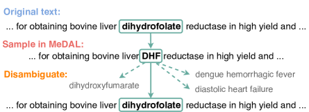
Figure 1: A sample in the MeDAL dataset.

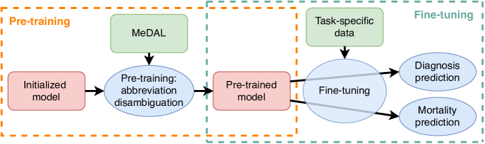
Figure 2: Diagram of using MeDAL for pre-training NLU models in medical domain.

The motivation behind using abbreviation disambiguation as the pre-training task is two-fold. First, abbreviations are widely used in medical records by healthcare professionals and can often be ambiguous (Xu et al., 2007; Islamaj Dogan et al., 2009). The ubiquitousness of abbreviations poses a restriction on building deep learning models for medical tasks, such as mortality prediction (Grnarova et al., 2016) and diagnosis prediction (Li et al., 2020).

Second, we believe that understanding natural language in a knowledge-rich domain such as medicine requires understanding of domain knowledge at some level, similar to how humans can understand medical text only after receiving medical training. The abbreviation disambiguation task enables models to use domain knowledge to understand the global and local context, as well as the possible meanings of the abbreviation in the medical domain.

Medical abbreviation disambiguation has long been studied (Skreta et al., 2019; Li et al., 2019; Finley et al., 2016; Liu et al., 2018; Joopudi et al., 2018; Jin et al., 2019) and our work builds upon many of them. In particular, our data generation process is inspired by the reverse substitution technique (Skreta et al., 2019; Finley et al., 2016).

Our work differs from them in mainly two aspects. First, instead of trying to improve performance on abbreviation disambiguation itself, we propose to use it as a pre-training task for transfer learning on other clinical tasks. Second, existing datasets for medical abbreviation disambiguation, for instance CASI (Moon et al., 2014), are small compared to datasets used for general language model pre-training, and as noted by Li et al. (2019) some are erroneous. Thus, we chose to construct a new dataset large enough for effective pre-training.

Our main contributions are: a) we present a large dataset for pre-training on the task of medical abbreviation disambiguation. b) we provide empirical evidence of the benefit of abbreviation pre-training for a wide range of deep learning architectures.

2 Abbreviation Disambiguation

2.1 Dataset Summary

The MeDAL dataset consists of 14,393,619 articles and on average 3 abbreviations per article. The statistics of MeDAL are summarized in Table 1.

The distribution of number of words and the distribution of number of abbreviations are shown in Figure 3(a) and Figure 3(b), respectively.

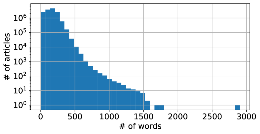
(a) Word count distribution

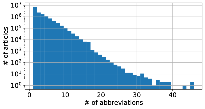
(b) Abbreviation count distribution

Figure 3: Distributions of number of words and number of abbreviations.

2.2 Dataset Creation

The MeDAL dataset is created from PubMed abstracts which are released in the 2019 annual baseline. PubMed is a search engine that indexes scientific publications in biomedical domain. The PubMed corpus contains 18,374,626 valid abstracts with 80 words in each abstract on average.

We use reverse substitution Skreta et al. (2019) to generate samples without human labeling. We identify full terms in text that have known abbreviations and replace them with their abbreviations. For reverse substitution, mappings of abbreviations to expansions established by Zhou et al. (2006) are used. Mappings where the abbreviation maps to only one expansion or the expansion maps to multiple abbreviations are discarded, resulting in 24,005 valid pairs of mappings. Among the valid mappings are 5,886 abbreviations, which means each abbreviation maps to about 4 expansions on average.

To avoid completely removing all expansions and making them unseen to models, the expansions are substituted with a pre-defined probability. For our study, expansions are substituted with a probability of $0.3$, although our processing scripts allow for other values for future use.

2.3 Pretraining

The task of abbreviation disambiguation is treated as a classification problem, where the classes are all possible expansions.

Considering the huge size of the dataset and the associated computational cost, a subset of 5 million data points are sampled from the complete corpus, which are split into 3 million training samples, 1 million validation samples and 1 million test samples. This subset is used throughout this study.

When creating this subset, because the distribution of true expansions is highly imbalanced, a sampling strategy is adopted which essentially removes classes in increasing order of frequency in an iterative manner. The sampling strategy works in the following way: from each class label, $N_{C}=min(F_{C},T)$ samples that have this label are randomly selected, where $F_{C}$ is the frequency of that class in the unsampled dataset, and $T$ is a threshold that is computed using Algorithm 1 such that each class can have at most $T$ samples, and $\sum_{C}N_{C}$ is equal to the total number of samples $N$.

The strategy iteratively removes classes, and at every iteration decreases $N^{\prime}$ (which corresponds to the number of remaining samples) and $L$ (which corresponds to the number of labels remaining). Then, the rate $r$ is calculated based on how many classes $L$ can fit in the remaining $N^{\prime}$ if each remaining $L$ has exactly $r$ samples. In this way, it is ensured that the moment the current class frequency $f_{C}$ being iterated is greater than the desired rate $r$, the sampling stops.

Algorithm 1 Compute threshold $T$

0:  array of class frequency $f$, $N>0$

  Sort $f$ in increasing order

  $L\leftarrow length(f)$

  $N^{\prime}\leftarrow N$

  for each $f_{C}\in f$ do

     $N^{\prime}\leftarrow N^{\prime}-f_{C}$

     $L\leftarrow L-1$

     $r=round(N^{\prime}/L)$

     if $f_{C}\geq r$ then

        return  $r+1$

     end if

  end for

3 Evaluation Tasks

total # of articles	14,393,619
median # of words	150
mean # of words	152.47
median # of abbreviations	2
mean # of abbreviations	3.04

Table 1: Statistics of the MeDAL dataset

Mortality Prediction

As a downstream task to evaluate models’ performance in clinical settings, mortality prediction aims at predicting the mortality of a patient at the end of a hospital admission, using ICU patient notes. The mortality prediction dataset is generated from MIMIC-III (Johnson et al., 2016). Medical notes in this MIMIC-III comprise of free-form text documents written by nurses, doctors, and many types of specialists, and are written throughout the patient’s stay. Only notes written by physicians and nurses at least twenty-four hours before the end of the discharge time are used, for the goal is to accurately predict whether a patient is at risk of dying by the end of the admission. In order to balance positive and negative samples (roughly 10% of patients expire at the end of an admission) while keeping as much text diversity as possible, we sample at most four notes from each surviving patient.

The dataset generated has a total of 137,607 negative samples and 138,864 positively-labelled notes. Then, using stratified random splitting, we selected 75%/10%/15% of the patients to be included in the training/validation/test splits. As an example of the ubiquitousness of abbreviations, ‘MR’ appears 1,612 times in 1,366 samples in the test set alone.

Diagnosis Prediction

Similar to mortality prediction, diagnosis prediction aims to predict the diagnoses associated with a hospital admission from medical notes written during the admission. The same MIMIC-III medical notes and the same splits from mortality prediction are used, with seven training samples that have no diagnosis recorded removed. In MIMIC-III, diagnoses are recorded with International Classification of Diseases (ICD) codes, which are standardized codes designed for billing purposes. We discard minor distinctions of ICD codes under the same category by taking the first three digits (for codes that start with ‘E’ or ‘V’ the first four digits) of ICD codes. After grouping, there are 1,204 unique diagnosis codes.

Top-k recall is used for evaluation of models based on the similarities to real-life medical decision making (Choi et al., 2015), which is defined as the number of diagnosis codes in that admission that are present in the top k predictions of the model, divided by the number of diagnosis codes in that admission in total. Note that since most admissions have multiple diagnoses, a small k would result in a top-k recall less than 100% even if all of the top k predictions are correct. On our dataset, the highest possible top-5, top-10 and top-30 recalls are $50.17\%$, $79.48\%$ and $99.88\%$ on validation set, and $49.75\%$, $79.23\%$ and $99.79\%$ on test set.

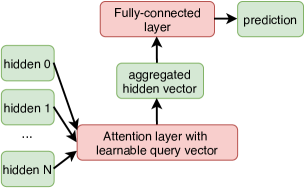
Figure 4: Attention output layer for mortality and diagnosis prediction.

4 Models

The models are first pre-trained on the MeDAL dataset, then pre-trained weights are used to initialize models for training on the downstream tasks. We compared this training strategy with training respective models from scratch to validate the benefit of pre-training.

LSTM

BiLSTM is used as a baseline model. Specifically, the BiLSTM consists of three layers with hidden size of 512. Pre-trained Fasttext model is used for word embeddings (Bojanowski et al., 2017).

LSTM + Self Attention

To allow for leveraging information extracted by LSTM in a flexible manner, soft attention layers are added on top of LSTM. The attention layer is largely based on the soft attention by Bahdanau et al. (2014). Its detailed formulation is included in Appendix A.

Transformers

We used the pre-trained ELECTRA-small discriminator (Clark et al., 2020) as an example of Transformer-based (Vaswani et al., 2017) model and, since it was not pre-trained on medical text, we compared its performance with or without pre-training on abbreviation disambiguation.

Task-specific Output Layer

Depending on the task, the output layer can take various forms. For abbreviation disambiguation, the output layer is a fully-connected layer, whose input is the hidden vector at the location of the abbreviation from the previous layers and output space is all possible expansions. For mortality or diagnosis prediction which are not associated with any specific token, hidden vectors from the previous layers need to be first aggregated into one vector. This can be achieved by either a pooling layer or an additional attention layer with a learnable query vector. Then the output layer is a fully connected layer that takes the aggregated vector as input. The attention output layer is illustrated in Figure 4. In preliminary experiments we found attention output layer generally improves models’ performance compared to max-pooling output layer, and therefore it is used throughout the rest of the study unless otherwise noted.

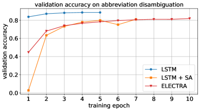
Figure 5: Validation accuracy on abbreviation disambiguation. ‘SA’ stands for self attention layer.

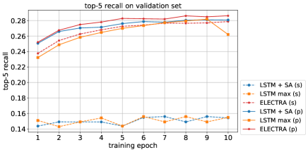
Figure 6: Top-5 recall on diagnosis prediction validation set. ‘SA’ stands for self attention layer. ‘max’ represents max-pooling output layer. ‘(s)’ and ‘(p)’ indicates whether the model is trained from scratch or pre-trained, respectively.

Model	Validation accuracy
	Pretrained	From scratch
LSTM	82.67%	82.17%
LSTM+SA	82.46%	80.29%
ELECTRA	84.19%	83.92%
	Test accuracy
LSTM	82.80%	82.61%
LSTM+SA	82.98%	79.96%
ELECTRA	84.43%	83.25%

Table 2: Results on mortality prediction. Bold font indicates the training strategy (pre-trained or from scratch) that has higher accuracy.

5 Results

Models’ performance on the pre-training task, abbreviation disambiguation, is shown in Figure 5. As the goal is not to optimize performance on this task, Figure 5 serves to confirm the models are properly pre-trained.

After pre-training, models are fine-tuned on the two downstream tasks to evaluate the benefit of pre-training. On the mortality prediction task, all three models that are pre-trained perform better than their from-scratch counterparts, shown in Table 2.

The benefit of pre-training is more significant on diagnosis prediction, shown in Figure 6. Both LSTM and LSTM + self attention perform considerably better if they pre-trained. In fact, the two models’ performance increase by more than 70% relatively. While for ELECTRA the gain is not as significant, pre-training leads to faster convergence during fine-tuning.

On the two downstream tasks, experiment results show that pre-training improves ELECTRA’s performance even when the model is already fully pre-trained on non-medical texts and is among the state-of-the-art, and bring the other models’ performance close to ELECTRA’s. This shows that pre-training on the MeDAL dataset can generally improves models capabilities of understanding language in medical domain. The complete results can be found in Appendix C.

6 Conclusion and Discussion

In this work, we present MeDAL, a large dataset on abbreviation disambiguation, designed for pre-training natural language understanding models in the medical domain. We pre-trained a variety of models using common architectures and empirically showed that such pre-training leads to improvement in performance as well as faster convergence when fine-tuning on two downstream clinical tasks.

Appendix A Attention Layer

Following Vaswani et al. (2017), the attention layer can be expressed in terms of key, query and value vectors, denoted as $\mathbf{k}_{i}$, $\mathbf{q}_{i}$ and $\mathbf{v}_{i}$ respectively, where the subscript $i$ denotes the location in the sequence. Specifically, the attention layer in our models is defined as Equation 1.

$$w_{ij}=\frac{\exp\alpha_{ij}}{\sum_{n}\exp\alpha_{in}}$$ (1)

$\alpha_{ij}$ in Equation 1 is computed with Equation 2, where $W_{a}$ and $b$ are learnable parameters.

$$\alpha_{ij}=\tanh(\mathbf{q}_{i}\cdot W_{a}\cdot{\mathbf{k}_{j}}^{T}+b)$$ (2)

Here $w_{ij}$ is the weight assigned to location $j$ for location $i$. Then the output of the attention layer at location $i$ is computed by taking the weighted sum of value vectors at all locations, i.e. $\mathbf{o}_{i}=\sum_{n}w_{in}\cdot\mathbf{v}_{n}$, where $\mathbf{o}_{i}$ denotes the output of attention layer at location $i$. Unless otherwise noted, throughout this paper $\mathbf{k}_{i}$, $\mathbf{q}_{i}$ and $\mathbf{v}_{i}$ are all equal to the hidden vector at position $i$ from the previous layer $\mathbf{h}_{i}$.

Appendix B Experiment Details

Except for ELECTRA, the rest of the models are trained with Adam optimizer (Kingma and Ba, 2014) with learning rate of $0.001$. Text is tokenized using pre-trained Fasttext embeddings (Bojanowski et al., 2017). All LSTM modules are bi-directional and have 3 layers, with hidden size of 512. Batch size is set to 64. We experimented with various choices of batch sizes, including 32, 64, 96 and 128, and noted only minimal differences. ELECTRA is trained with Adam optimizer with learning rate of $0.00002$ and with batch size of 16.

Appendix C Additional Experiments Results

Figure 7 to Figure 8 show the top-10, and top-30 recalls on diagnosis prediction, respectively. Table 3 shows the complete performance of models on diagnosis prediction.

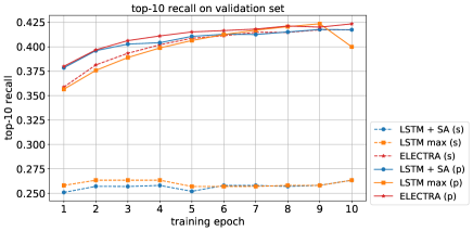
Figure 7: Top-10 recall on diagnosis prediction validation set. ‘SA’ stands for self attention layer. ‘max’ represents max-pooling output layer. ‘(s)’ and ‘(p)’ indicates whether the model is trained from scratch or pre-trained, respectively.

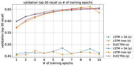
Figure 8: Top-30 recall on diagnosis prediction validation set. ‘SA’ stands for self attention layer. ‘max’ represents max-pooling output layer. ‘(s)’ and ‘(p)’ indicates whether the model is trained from scratch or pre-trained, respectively.

Model	Validation performance
	Top-5 recall		Top-10 recall		Top-30 recall
	Pre-trained	From scratch	Pre-trained	From scratch	Pre-trained	From scratch
LSTM	26.20%	15.49%	40.00%	26.33%	63.57%	45.78%
LSTM+SA	28.08%	15.43%	41.75%	26.33%	65.15%	46.33%
Electra	28.63%	28.08%	42.35%	41.74%	65.64%	65.37%
	Test performance
LSTM	26.94%	15.67%	40.59%	25.97%	65.49%	45.15%
LSTM+SA	27.47%	15.93%	41.24%	25.97%	65.86%	45.67%
Electra	27.88%	27.90%	41.76%	41.82%	66.23%	66.49%

Table 3: Performance on diagnosis prediction^ab

• Note that, as discussed in Section 3, on our dataset the highest possible top-5, top-10 and top-30 recalls are $50.17\%$, $79.48\%$ and $99.88\%$ on validation set, and $49.75\%$, $79.23\%$ and $99.79\%$ on test set.

• Bold font indicates the training strategy (pre-trained or from scratch) that has higher accuracy.

References

- Bahdanau et al. (2014) Dzmitry Bahdanau, Kyunghyun Cho, and Yoshua Bengio. 2014. Neural Machine Translation by Jointly Learning to Align and Translate.
- Bojanowski et al. (2017) Piotr Bojanowski, Edouard Grave, Armand Joulin, and Tomas Mikolov. 2017. Enriching Word Vectors with Subword Information. Transactions of the Association for Computational Linguistics, 5:135–146.
- Choi et al. (2015) Edward Choi, Mohammad Taha Bahadori, Andy Schuetz, Walter F. Stewart, and Jimeng Sun. 2015. Doctor AI: Predicting Clinical Events via Recurrent Neural Networks.
- Clark et al. (2020) Kevin Clark, Minh-Thang Luong, Quoc V. Le, and Christopher D. Manning. 2020. ELECTRA: Pre-training Text Encoders as Discriminators Rather Than Generators. In International Conference on Learning Representations.
- Finley et al. (2016) Gregory P. Finley, Serguei V.S. Pakhomov, Reed McEwan, and Genevieve B. Melton. 2016. Towards Comprehensive Clinical Abbreviation Disambiguation Using Machine-Labeled Training Data. AMIA … Annual Symposium proceedings. AMIA Symposium, 2016:560–569.
- Grnarova et al. (2016) Paulina Grnarova, Florian Schmidt, Stephanie L. Hyland, and Carsten Eickhoff. 2016. Neural Document Embeddings for Intensive Care Patient Mortality Prediction.
- Islamaj Dogan et al. (2009) R. Islamaj Dogan, G. C. Murray, A. Neveol, and Z. Lu. 2009. Understanding PubMed(R) user search behavior through log analysis. Database, 2009(0):bap018–bap018.
- Jin et al. (2019) Qiao Jin, Jinling Liu, and Xinghua Lu. 2019. Deep Contextualized Biomedical Abbreviation Expansion. In BioNLP 2019, pages 88–96. Association for Computational Linguistics (ACL).
- Johnson et al. (2016) Alistair E.W. Johnson, Tom J. Pollard, Lu Shen, Li Wei H. Lehman, Mengling Feng, Mohammad Ghassemi, Benjamin Moody, Peter Szolovits, Leo Anthony Celi, and Roger G. Mark. 2016. MIMIC-III, a freely accessible critical care database. Scientific Data, 3(1):1–9.
- Joopudi et al. (2018) Venkata Joopudi, Bharath Dandala, and Murthy Devarakonda. 2018. A convolutional route to abbreviation disambiguation in clinical text. Journal of Biomedical Informatics, 86:71–78.
- Kingma and Ba (2014) Diederik P. Kingma and Jimmy Ba. 2014. Adam: A Method for Stochastic Optimization.
- Li et al. (2019) Irene Li, Michihiro Yasunaga, Muhammed Yavuz Nuzumlalı, Cesar Caraballo, Shiwani Mahajan, Harlan Krumholz, and Dragomir Radev. 2019. A Neural Topic-Attention Model for Medical Term Abbreviation Disambiguation.
- Li et al. (2020) Yue Li, Pratheeksha Nair, Xing Han Lu, Zhi Wen, Yuening Wang, Amir Ardalan Kalantari Dehaghi, Yan Miao, Weiqi Liu, Tamas Ordog, Joanna M. Biernacka, Euijung Ryu, Janet E. Olson, Mark A. Frye, Aihua Liu, Liming Guo, Ariane Marelli, Yuri Ahuja, Jose Davila-Velderrain, and Manolis Kellis. 2020. Inferring multimodal latent topics from electronic health records. Nature communications, 11(1):2536.
- Liu et al. (2018) Yue Liu, Tao Ge, Kusum S. Mathews, Heng Ji, and Deborah L. McGuinness. 2018. Exploiting Task-Oriented Resources to Learn Word Embeddings for Clinical Abbreviation Expansion. In BioNLP 2015.
- Moon et al. (2014) Sungrim Moon, Serguei Pakhomov, Nathan Liu, James O Ryan, and Genevieve B Melton. 2014. A sense inventory for clinical abbreviations and acronyms created using clinical notes and medical dictionary resources. Journal of the American Medical Informatics Association, 21(2):299–307.
- Skreta et al. (2019) Marta Skreta, Aryan Arbabi, Jixuan Wang, and Michael Brudno. 2019. Training without training data: Improving the generalizability of automated medical abbreviation disambiguation.
- Vaswani et al. (2017) Ashish Vaswani, Noam Shazeer, Niki Parmar, Jakob Uszkoreit, Llion Jones, Aidan N. Gomez, Lukasz Kaiser, and Illia Polosukhin. 2017. Attention Is All You Need.
- Wang et al. (2018) Yanshan Wang, Liwei Wang, Majid Rastegar-Mojarad, Sungrim Moon, Feichen Shen, Naveed Afzal, Sijia Liu, Yuqun Zeng, Saeed Mehrabi, Sunghwan Sohn, and Hongfang Liu. 2018. Clinical information extraction applications: A literature review.
- Xu et al. (2007) Hua Xu, Peter D. Stetson, and Carol Friedman. 2007. A study of abbreviations in clinical notes. AMIA … Annual Symposium proceedings / AMIA Symposium. AMIA Symposium, 2007:821–825.
- Zhou et al. (2006) W. Zhou, V. I. Torvik, and N. R. Smalheiser. 2006. ADAM: another database of abbreviations in MEDLINE. Bioinformatics, 22(22):2813–2818.