On the three-particle analog of the Lellouch-Lüscher formula

Abstract

Using non-relativistic effective field theory, we derive a three-particle analog of the Lellouch-Lüscher formula at the leading order. This formula relates the three-particle decay amplitudes in a finite volume with their infinite-volume counterparts and, hence, can be used to study the three-particle decays on the lattice. The generalization of the approach to higher orders is briefly discussed.

1 Introduction

Back in 2000, Lellouch and Lüscher Lellouch:2000pv derived a formula, which related the matrix element of the weak $K\to 2\pi$ decay in a finite volume to its infinite-volume counterpart. These two quantities turn out to be proportional with a factor (Lellouch-Lüscher (LL) factor), depending on the size $L$ of a cubic box and on the elastic two-body pion-pion scattering phase shift. The result of Ref. Lellouch:2000pv paved the way to the systematic studies of various two-body decays on the lattice. Later, different generalizations of the method emerged, e.g., for moving frames Kim:2005gf ; Christ:2005gi , or for the case of coupled two-body channels Hansen:2012tf . A simple and transparent derivation of the LL formula with the use of the non-relativistic effective Lagrangians has been given in Bernard:2012bi . For the application of the formalism, we refer here, e.g., to a comprehensive study of the $K\to\pi\pi$ decays, which has been carried out recently by the RBC and UKQCD Collaborations Abbott:2020hxn . From the related work, we mention the study of the matrix elements of currents, corresponding to the $1\to 2$ transition Briceno:2015csa ; Briceno:2014uqa , and of the timelike pion form factor Meyer:2011um , which all feature the similar factor in a finite volume. Generally, in the LL type formulae, this $L$-dependent factor emerges from the multiple rescattering of two particles in the final state (pions), and the phase shift, which also enters the expression, should be measured on the same lattice, simultaneously with the measurement of the decay matrix element. It can be done by using the Lüscher formula that relates the phase shift to the volume-dependent spectrum in the two-particle sector.

To summarize, the two-body problem is completely understood from the conceptual point of view – both the scattering, as well as two-body decays. On the contrary, the three-body formalism is still in development. Recently, three physically equivalent forms of the quantization condition have been proposed Hansen:2014eka ; Hansen:2015zga ; Hammer:2017uqm ; Hammer:2017kms ; Mai:2017bge , which relate the three-body spectrum in a finite volume with the infinite-volume parameters in the three-body sector. However, in contrast to the two-body case, where the Lüscher equation enables one to extract the two-body phase shift from the measured spectrum in one step, the procedure in the three-particle sector is more complicated. To start with, the three-body quantization condition becomes tractable only if the three-body interactions are expressed in terms of few parameters. In the approach of Refs. Hammer:2017uqm ; Hammer:2017kms , such a parameterization naturally emerges, when the three-body interactions are evaluated from the effective Lagrangian at tree level that allows one to impose a consistent power counting. Similarly, the three-body kernels in the approaches of Refs. Hansen:2014eka ; Hansen:2015zga and Ref. Mai:2017bge can be expanded in the external momenta (up to a given order) in the vicinity of the threshold. Thus, the fit of the quantization condition to the three-particle spectrum, which is measured on the lattice, enables one to extract few parameters (the effective three-particle couplings, or the coefficients in the expansion of the three-particle kernel). These can be substituted into the infinite-volume equations to calculate observables in the three-particle sector. Consequently, extracting the three-particle observables from data necessarily involves an intermediate step, and cannot be done directly, as in case of two particles.

It should be mentioned that the above theoretical developments have largely boosted the study of three (and more particles) on the lattice, be this in QCD or other field-theoretical models Beane:2007es ; Horz:2019rrn ; Culver:2019vvu ; Fischer:2020jzp ; Blanton:2019vdk ; Hansen:2020otl ; Alexandru:2020xqf ; Romero-Lopez:2018rcb ; Romero-Lopez:2020rdq . In view of these activities, the need for the three-particle analog of the LL formula, which should be used for the extraction of the matrix elements, becomes obvious. Such a formula, however, was not available in the literature so far. Moreover, bearing in mind the above discussion, it is not even clear, whether the relation between the finite- and infinite-volume matrix elements, which one is after, should contain a single overall factor (a counterpart of the LL factor), or should be more complicated. On the other hand, recent years have seen a growing interest to the study of three-particle decays. The most obvious candidates for this study in the beginning are provided by the three-pion decays of low-mass light-flavored mesons $K\to 3\pi$, $\eta\to 3\pi$ and $\omega\to 3\pi$. The decays of the heavier pseudovector mesons $a_{1}(1260)\to\rho\pi\to 3\pi$ and $a_{1}(1420)\to f_{0}(980)\pi\to 3\pi$ are also very interesting. Further, the candidates for exotica, $X(3872)$ and $X(4260)$, decay largely into the three-particle final states as well. Last but not least, the extraction of the parameters of the Roper resonance on the lattice has proven to be very challenging. That might be, in part, related to the lack of proper treatment of the three-particle decay channel in a finite volume. Our paper intends to make the first step towards the creation of a systematic finite-volume framework for the study of three-body decays on the lattice that will contribute to the solution of the above-mentioned problems.

Note that the resonances, which are studied in lattice QCD, fall into two categories. To the first category belong the ones, which are stable in pure QCD, like kaons that decay through weak interactions. Further, the $\eta$-mesons are not stable in QCD. However, the decay amplitude is proportional to the $u$- and $d$-quark mass difference $m_{u}-m_{d}$ and thus vanishes in the isospin limit. So, if one wants to know this amplitude only at the first order in $m_{u}-m_{d}$ (this completely suffices for practical reasons), one could also formally categorize this decay into the first group and treat the final state interactions in the isospin-symmetric QCD, where the $\eta$-mesons are stable. The second, larger group consists of the genuine QCD resonances. In this paper, like in the original paper by Lellouch and Lüscher, we concentrate our effort on the first group. The treatment of the QCD resonances is a more subtle issue that includes, in particular, analytic continuation into the complex energy plane to the resonance pole. In the case of two-body decays, this procedure is discussed, in particular, in Refs. Bernard:2012bi ; Agadjanov:2014kha ; Agadjanov:2016fbd ; Briceno:2015dca ; Briceno:2016kkp . We postpone the discussion of a similar procedure in the three-particle sector to our future investigations.

The layout of the paper is as follows: In Sect. 2, we display the lowest-order non-relativistic effective Lagrangian and write down the quantization condition in a finite volume. In Sect. 3, we derive the LL equation at leading order. The extension of the approach to higher orders is discussed in Sect. 4. Section 5 contains our conclusions.

2 Non-relativistic framework

The non-relativistic EFT framework, which was tailored to study the singularity structure of the amplitudes in three-body decays, was proposed in Ref. Colangelo:2006va . It has been successfully used in the study of the three-body decays of charged and neutral kaons, as well as $\omega,\eta$ and $\eta^{\prime}$ mesons Bissegger:2008ff ; Bissegger:2007yq ; Gullstrom:2008sy ; Schneider:2010hs ; Kubis:2009sb . A brief review of the essential points of the approach is given in Ref. Gasser:2011ju . The main difference of this approach from the conventional ones consists in the treatment of the relativistic corrections to the internal particle lines. Whereas in the conventional approach, these corrections are treated perturbatively, in the new one they are summed up to all orders, ensuring the correct relativistic dispersion law. As a result, the location of singularities in the decay amplitude stays fixed to all orders and coincides with the singularity structure of the relativistic amplitude. There is a price to pay for this, however: the resummed propagators feature the hard scale – the particle mass – explicitly. This, as known, leads to the breakdown of the naive counting rules. In order to rectify the counting rules, one then has to amend the procedure for the calculation of the Feynman integrals – dimensional regularization plus minimal subtraction does not suffice. The modification of the procedure, which is equivalent to the change of the renormalization prescription, is described in detail in Gasser:2011ju , and we refer an interested reader to that article.

To purify the problem from the inessential details as much as possible, we shall consider below a decay of a spinless particle (“kaon”) into three likewise spinless particles (“pions”). Isospin and other quantum numbers are discarded. We also assume that there exists some discrete symmetry (like $G$-parity), which forbids transitions with an odd number of the external pion legs. The non-relativistic fields $K(x)$ and $\phi(x)$ describe kaons and pions, respectively, and $M,m$ denote their masses. The lowest-order Lagrangian, which describes the decay, is given by

$$\mathcal{L} = K^{\dagger}2W(i\partial_{t}-W)K+\phi^{\dagger}2w(i\partial_{t}-w)\phi$$ (1)

$$+ \frac{C_{0}}{4}\phi^{\dagger}\phi^{\dagger}\phi\phi+\frac{D_{0}}{36}\phi^{\dagger}\phi^{\dagger}\phi^{\dagger}\phi\phi\phi+\frac{G_{0}}{6}\left(K^{\dagger}\phi\phi\phi+\text{h.c.}\right)\,,$$

where $W=\sqrt{M^{2}-\nabla^{2}}$ and $w=\sqrt{m^{2}-\nabla^{2}}$.

In the above Lagrangian, the constant $G_{0}$ describes the elementary act of the kaon decay into three pions. It is proportional to the weak coupling constant and enters the amplitudes, by definition, only at the first order. If the weak interactions are switched off, the kaon is stable. Further, the constants $C_{0}$ and $D_{0}$ describe the strong final state interactions in the system of two and three pions respectively. Unlike the constant $G_{0}$, these enter the expression of the amplitude at all orders. The matching at the two-pion threshold relates the constant $C_{0}$ to the pion-pion scattering length $a$:

$$C_{0}=-32\pi am\,.$$ (2)

In Eq. (1), only the leading-order terms are displayed. The power counting at the Lagrangian level is defined by the (formal) requirement that all three-momenta count at $O(p)$, whereas the kinetic energies of the individual pions, as well as the quantity $M-3m$ count at $O(p^{2})$. The higher-order Lagrangians would contain an even number of spatial derivatives, acting on all fields. Below, we shall concentrate on the derivation of the LL formula at the leading order, using the Lagrangian in Eq. (1). The inclusion of the higher-order terms will be considered briefly in Sect. 4.

Moreover, in order to write down the equation that determines the three-particle scattering amplitude, we shall switch to the particle-dimer picture. It is well-known that this formulation, which is equivalent to the original one, enables one to drastically simplify the bookkeeping of Feynman diagrams and arrive at the result with a surprising ease Kaplan:1996nv ; Bedaque:1998kg ; Bedaque:1998km . The Lagrangian in the particle-dimer picture in our case is given by:

$$\mathcal{L} = K^{\dagger}2W(i\partial_{t}-W)K+\phi^{\dagger}2w(i\partial_{t}-w)\phi+\sigma d^{\dagger}d$$ (3)

$$+ \frac{f_{0}}{2}\left(d^{\dagger}\phi\phi+\text{h.c.}\right)+h_{0}d^{\dagger}d\phi^{\dagger}\phi+g_{0}\left(K^{\dagger}d\phi+\text{h.c.}\right)\,.$$

Here, $d$ denotes the dimer field, and $\sigma=\pm 1$, depending on the sign of the constant $C_{0}$. Integrating out the field $d$ in the path integral and expanding in the powers of fields, one arrives at the Lagrangian, given in Eq. (1), if the following relations are fulfilled:

$$\sigma f_{0}^{2}=-C_{0},\qquad 9f_{0}^{2}h_{0}=D_{0},\qquad 3\sigma f_{0}g_{0}=-G_{0}\,.$$ (4)

We would like to stress here that the validity of the particle-dimer picture does not imply that a two-body bound state really exists. As one sees, the dimer field is introduced in the path integral as a dummy integration variable and, hence, the resulting formulation is mathematically equivalent to the initial one without a dimer field. If a dimer (or a narrow low-lying resonance) indeed exists, this may affect only the convergence of the expansion. In this case, the bulk of the two-particle interaction will be described by the dimer exchange in the $s$-channel, and the contribution from the higher orders will be small.

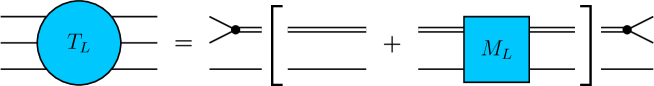
Figure 1: Expressing the three-particle scattering amplitude through the particle-dimer scattering amplitude, see Eq. (13). The single and double lines are the particle and the dimer propagators, respectively, and the filled circle denotes the two-particle-dimer vertex.

The Lagrangian (3) will be used for the calculation of the Feynman diagrams in a finite volume – as it is well-known, the sole change is the replacement of the infinite-momentum integrals by the sums over the discrete three-momenta of particles in a finite cubic box. The propagator of the non-relativistic field $\phi(x)$ in a finite volume is given by:

$$i\langle 0|T\phi(x)\phi^{\dagger}(y)|0\rangle=\int\frac{dp_{0}}{2\pi}\phantom{.}\frac{1}{L^{3}}\sum_{\mathbf{p}}\frac{e^{-ip_{0}(x_{0}-y_{0})+i\mathbf{p}(\mathbf{x}-\mathbf{y})}}{2w(\mathbf{p})(w(\mathbf{p})-p_{0}-i\varepsilon)}\,,\qquad w(\mathbf{p})=\sqrt{m^{2}+\mathbf{p}^{2}}\,.\quad$$ (5)

The dimer propagator is obtained by summing pion loops to all orders:

$$i\langle 0|Td(x)d^{\dagger}(y)|0\rangle=\int\frac{dP_{0}}{2\pi}\phantom{.}\frac{1}{L^{3}}\sum_{\mathbf{P}}e^{-iP_{0}(x_{0}-y_{0})+i\mathbf{P}(\mathbf{x}-\mathbf{y})}\,D_{L}(\mathbf{P};P_{0})\,.$$ (6)

Here $D_{L}$ obeys the following equation:

$$D_{L}(\mathbf{P};P_{0})=-\frac{1}{\sigma}-\frac{f_{0}^{2}}{2\sigma}\,J_{L}(\mathbf{P};P_{0})D_{L}(\mathbf{P};P_{0})\,,$$ (7)

where $J_{L}$ denotes a single pion loop:

$$J_{L}(\mathbf{P};P_{0}) = \frac{1}{L^{3}}\sum_{\mathbf{k}}\frac{1}{4w(\mathbf{k})w(\mathbf{P}-\mathbf{k})(w(\mathbf{k})+w(\mathbf{P}-\mathbf{k})-P_{0}-i\varepsilon)}$$ (8)

$$= \frac{p^{*}}{8\pi^{5/2}\sqrt{s}\gamma\eta}Z^{\mathbf{d}}_{00}(1;s)\,,$$

and

$$s=P_{0}^{2}-\mathbf{P^{2}},\quad\gamma=\frac{P_{0}}{\sqrt{s}}\,,\quad p^{*}=\sqrt{\frac{s}{4}-m^{2}},\quad\eta=\frac{p^{*}L}{2\pi}\,,\quad\mathbf{d}=\frac{\mathbf{P}L}{2\pi}\,.$$ (9)

Further, in Eq. (8), $Z^{\mathbf{d}}_{00}(1;s)$ is the usual Lüscher zeta function, boosted to the moving frame defined by the vector $\mathbf{d}$. For a general $(lm)$, this function is given by:

$$Z^{\mathbf{d}}_{lm}(1;s)=\sum_{\mathbf{r}\in P_{d}}\frac{\mathcal{Y}_{lm}(\mathbf{r})}{\mathbf{r}^{2}-\eta^{2}}\,,\quad P_{d}=\left\{\mathbf{r}\in\mathbb{R}^{3}\biggl{|}r_{\parallel}=\gamma^{-1}\left(n_{\parallel}-|{\bf d}|/2\right)\,,~{}\mathbf{r}_{\perp}=\mathbf{n}_{\perp}\,,~{}\mathbf{n}\in\mathbb{Z}^{3}\right\}\,,$$

where $\mathcal{Y}_{lm}(\mathbf{r})=|\mathbf{r}|^{l}Y_{lm}(\hat{r})$, and $Y_{lm}(\hat{r})$ denotes the usual spherical function that depends on the unit vector $\hat{r}$. Finally, after using the matching condition, for the dimer propagator one obtains:

$$D_{L}(\mathbf{P};P_{0})=\frac{\sigma\sqrt{s}/(2am)}{-\sqrt{s}/(2am)+p^{*}\cot\phi^{\mathbf{d}}(s)},\quad\quad\cot\phi^{\mathbf{d}}(s)=-\frac{Z_{00}^{\mathbf{d}}(1;s)}{\pi^{3/2}\gamma\eta}\,.$$ (11)

In the non-relativistic limit, $\sqrt{s}/(2m)\to 1$, $\gamma\to 1$, and we arrive at the expression displayed in Refs. Hammer:2017uqm ; Hammer:2017kms . At higher orders, the expression $-1/a$ both in the numerator and the denominator gets replaced by $p^{*}\cot\delta(p^{*})=-1/a+r{p^{*}}^{2}/2+\ldots$. Further, the infinite-volume counterpart of Eq. (11) reads:

$$D(\mathbf{P};P_{0})=\frac{\sigma\sqrt{s}/(2am)}{-\sqrt{s}/(2am)-ip^{*}}\,.$$ (12)

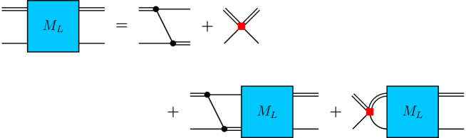
Figure 2: The Faddeev equation for the particle-dimer scattering amplitude. The red shaded squares denote the particle-dimer coupling.

The finite-volume energy levels in the three-particle system coincide with the location of the poles of the three-particle scattering amplitude. In the particle-dimer picture, this quantity can be directly related to the particle-dimer scattering amplitude Hammer:2017uqm ; Hammer:2017kms ; Doring:2018xxx , see Fig. 1. At the lowest order, the relation is given by:

$$T_{L}(\{\mathbf{p}\},\{\mathbf{q}\};P_{0}) = \sum\limits_{\alpha,\beta=1}^{3}\biggl{[}\tau_{L}(-\mathbf{p}_{\alpha};P_{0})2w(\mathbf{p}_{\alpha})L^{3}\delta_{\mathbf{p}_{\alpha}\mathbf{q}_{\beta}}$$ (13)

$$+ \tau_{L}(-\mathbf{p}_{\alpha};P_{0})M_{L}(-\mathbf{p}_{\alpha},-\mathbf{q}_{\beta};P_{0})\tau_{L}(-\mathbf{q}_{\beta};P_{0})\biggr{]}\,,$$

where $\{\mathbf{p}\}$ stands for the set of all three particle momenta $\mathbf{p}_{\alpha}$ with $\alpha=1,2,3$. In the center-of-mass frame, the dimer momenta are equal to $-\mathbf{p}_{\alpha}$. The sets $\{\mathbf{q}\}$, $\{\mathbf{k}\}$ are defined similarly. Further,

$$\tau_{L}(\mathbf{p};P_{0})=f_{0}^{2}D_{L}(\mathbf{p};P_{0}-w(\mathbf{p}))\,.$$ (14)

In the infinite volume, the relation between the quantities $\tau(\mathbf{p};P_{0})$ and $D(\mathbf{p};P_{0})$ takes a similar form. Further, $M_{L}(\mathbf{p},\mathbf{q};P_{0})$ denotes the particle-dimer scattering amplitude, which obeys the Faddeev equation in a finite volume, see Fig. 2:

$$M_{L}(\mathbf{p},\mathbf{q};P_{0})=Z(\mathbf{p},\mathbf{q};P_{0})+\frac{1}{L^{3}}\sum_{\mathbf{k}}^{\Lambda}Z(\mathbf{p},\mathbf{k};P_{0})\frac{\tau_{L}(\mathbf{k};P_{0})}{2w(\mathbf{k})}M_{L}(\mathbf{k},\mathbf{q};P_{0})\,,$$ (15)

where $\Lambda$ denotes an ultraviolet cutoff and

$$Z(\mathbf{p},\mathbf{q};P_{0})=\left[\frac{1}{2w(\mathbf{p}+\mathbf{q})(w(\mathbf{p}+\mathbf{q})+w(\mathbf{p})+w(\mathbf{q})-P_{0}-i\varepsilon)}+\frac{h_{0}}{f_{0}^{2}}\right]\,.$$ (16)

In the infinite volume, the Faddeev equation becomes the integral equation with the same kernel $Z$ and cutoff $\Lambda$:

$$M(\mathbf{p},\mathbf{q};P_{0})=Z(\mathbf{p},\mathbf{q};P_{0})+\int^{\Lambda}\frac{d^{3}\mathbf{k}}{(2\pi)^{3}}\,Z(\mathbf{p},\mathbf{k};P_{0})\frac{\tau(\mathbf{k};P_{0})}{2w(\mathbf{k})}M(\mathbf{k},\mathbf{q};P_{0})\,.$$ (17)

The quantization condition in a finite volume takes the form:

$$\mbox{det}(A)=0\,,\qquad A_{\mathbf{p}\mathbf{q}}=2w(\mathbf{p})\tau_{L}^{-1}(\mathbf{p};P_{0})L^{3}\delta_{\mathbf{p}\mathbf{q}}-Z(\mathbf{p},\mathbf{q};P_{0})\,.$$ (18)

The discrete solutions $P_{0}=E_{n}$ of the quantization condition determine the finite-volume spectrum of the three-particle system. Further, in the vicinity of a pole $P_{0}=E_{n}$, the residue of the particle-dimer amplitude factorizes:

$$M_{L}(\mathbf{p},\mathbf{q};P_{0})\biggr{|}_{P_{0}\to E_{n}}=\frac{\psi_{L}^{(n)}(\mathbf{p})\psi_{L}^{(n)}(\mathbf{q})}{E_{n}-P_{0}}+\mbox{regular}\,.$$ (19)

The particle-dimer wave function obeys a homogeneous equation:

$$\psi_{L}^{(n)}(\mathbf{p})=\frac{1}{L^{3}}\sum_{\mathbf{k}}^{\Lambda}Z(\mathbf{p},\mathbf{k};E_{n})\frac{\tau_{L}(\mathbf{k};E_{n})}{2w(\mathbf{k})}\psi_{L}^{(n)}(\mathbf{k})\,.$$ (20)

The normalization condition for the finite-volume wave function $\psi^{(n)}_{L}({\bf p})$ can be derived in a standard manner by using Eqs. (17), (19) and (20). Since both $Z$ and $\tau_{L}$ are energy-dependent, $\psi_{L}({\bf p})$ is not merely normalized to unity. Instead, the normalization condition takes the form:

$$\frac{1}{L^{6}}\sum_{{\bf p},{\bf k}}^{\Lambda}\psi^{(n)}({\bf p})\frac{\tau_{L}(\mathbf{p};E_{n})}{2w(\mathbf{p})}\,\frac{dZ({\bf p},{\bf k};E_{n})}{dE_{n}}\,\frac{\tau_{L}(\mathbf{k};E_{n})}{2w(\mathbf{k})}\,\psi^{(n)}_{L}({\bf k})$$

$$\quad+\frac{1}{L^{3}}\sum_{\bf p}^{\Lambda}\psi^{(n)}({\bf p})\frac{1}{2w(\mathbf{p})}\,\frac{d\tau_{L}(\mathbf{p};E_{n})}{dE_{n}}\,\psi^{(n)}_{L}({\bf p})=1\,.$$ (21)

The three-particle scattering amplitude factorizes as well:

$$T_{L}(\{\mathbf{p}\},\{\mathbf{q}\};P_{0})\biggr{|}_{P_{0}\to E_{n}}=\frac{\Psi_{L}^{(n)}(\{\mathbf{p}\})\Psi_{L}^{(n)}(\{\mathbf{q}\})}{E_{n}-P_{0}}+\mbox{regular}\,,$$ (22)

where

$$\Psi_{L}^{(n)}(\{\mathbf{p}\})=\sum_{\alpha=1}^{3}\tau_{L}(-\mathbf{p}_{\alpha};E_{n})\psi_{L}^{(n)}(-\mathbf{p}_{\alpha})\,.$$ (23)

Up to the change to the relativistic normalization and the use of the relativistic kinematics in the dimer propagator, these equations are equivalent to the ones displayed in Refs. Hammer:2017uqm ; Hammer:2017kms ; Doring:2018xxx . The numerical solution of similar equations in a finite volume has been considered also, e.g., in Refs. Kreuzer:2010ti ; Kreuzer:2009jp ; Kreuzer:2008bi ; Kreuzer:2012sr .

3 Derivation of the three-particle analog of the LL formula at the leading order

The derivation of the counterpart of the LL formula in the three-particle sector proceeds along the path already used in the two-particle case Bernard:2012bi . The main idea can be formulated in few words. The non-relativistic effective Lagrangians, used to describe physics in the infinite and in a finite volume, are the same. At the leading order, the only unknown, which can be extracted from the measured $K\to 3\pi$ decay matrix element on the lattice, is the coupling $G_{0}$ (other couplings, $C_{0}$ and $D_{0}$, can be independently determined by measuring the two- and three-body energy levels). Hence, the only thing that one has to do is to calculate the decay matrix elements in the effective theory twice: in a finite and in the infinite volume. Since at the leading order this matrix element is merely proportional to $G_{0}$, in the ratio of the results of the two calculations, which is the three-particle analog of the LL factor we are looking for, this constant drops out. Thus, the final answer is expressed solely in terms of known constants $C_{0}$ and $D_{0}$.

The crucial point in this derivation is to concentrate on $G_{0}$ which, by definition, is the same in a finite and in the infinite volume, up to the exponentially suppressed corrections. In these corrections, the hard scale of the effective theory appears in the argument of the exponent (in our case, this hard scale is given by the pion mass $m$). On the contrary, the measured matrix element contains a non-trivial, power-law $L$-dependence, which emerges via the final state interactions. Hence, no regular $L\to\infty$ limit exists for this matrix element.

After this introductory remark, we proceed with the calculation of the decay matrix element. Following Ref. Bernard:2012bi , first, one has to calculate the wave function renormalization constant for the composite operator $\mathcal{O}(x_{0};\{\mathbf{k}\})$, which creates three pions with momenta $\mathbf{k}_{1},\mathbf{k}_{2},\mathbf{k}_{3}$, acting on the vacuum bra-vector $\langle 0|$:

$$\mathcal{O}(x_{0};\{\mathbf{k}\})=\int d^{3}\mathbf{x}_{1}d^{3}\mathbf{x}_{2}d^{3}\mathbf{x}_{3}\phantom{.}e^{-i\mathbf{k}_{1}\mathbf{x}_{1}-i\mathbf{k}_{2}\mathbf{x}_{2}-i\mathbf{k}_{3}\mathbf{x}_{3}}\phi(x_{0},\mathbf{x}_{1})\phi(x_{0},\mathbf{x}_{2})\phi(x_{0},\mathbf{x}_{3})\,.$$ (24)

Assume now that $x_{0}>y_{0}$. Inserting a complete set of the intermediate states, for the two-body correlator one gets:

$$\langle 0|\mathcal{O}(x_{0};\{\mathbf{k}\})\mathcal{O}^{\dagger}(y_{0};\{\mathbf{k}\})|0\rangle=\sum_{n}\left|\langle 0|\mathcal{O}(0;\{\mathbf{k}\})|n\rangle\right|^{2}e^{-iE_{n}(x_{0}-y_{0})}\,.$$ (25)

On the other hand, one can evaluate this correlator in the perturbation theory. Summing up all diagrams, one obtains:

$$\langle 0|\mathcal{O}(x_{0};\{\mathbf{k}\})\mathcal{O}^{\dagger}(y_{0};\{\mathbf{k}\})|0\rangle=\int\frac{dP_{0}}{2\pi i}\phantom{.}e^{-iP_{0}(x_{0}-y_{0})}$$ (26)

$$\times \biggl{\{}\frac{L^{9}\left(1+\delta_{\mathbf{k}_{1}\mathbf{k}_{2}}+\delta_{\mathbf{k}_{1}\mathbf{k}_{3}}+\delta_{\mathbf{k}_{2}\mathbf{k}_{3}}+2\delta_{\mathbf{k}_{1}\mathbf{k}_{2}}\delta_{\mathbf{k}_{2}\mathbf{k}_{3}}\right)}{8w(\mathbf{k}_{1})w(\mathbf{k}_{2})w(\mathbf{k}_{3})(w(\mathbf{k}_{1})+w(\mathbf{k}_{2})+w(\mathbf{k}_{3})-P_{0}-i\varepsilon)}$$

$$+ \frac{L^{3}T_{L}(\{\mathbf{k}\},\{\mathbf{k}\};P_{0})}{\left(8w(\mathbf{k}_{1})w(\mathbf{k}_{2})w(\mathbf{k}_{3})(w(\mathbf{k}_{1})+w(\mathbf{k}_{2})+w(\mathbf{k}_{3})-P_{0}-i\varepsilon)\right)^{2}}\biggr{\}}\,.$$

Using Eq. (22) and performing contour integration by means of the Cauchy theorem, one gets:

$$\langle 0|\mathcal{O}(x_{0};\{\mathbf{k}\})\mathcal{O}^{\dagger}(y_{0};\{\mathbf{k}\})|0\rangle=\sum_{n}\frac{e^{-iE_{n}(x_{0}-y_{0})}L^{3}\left(\Psi_{L}^{(n)}(\{\mathbf{k}\})\right)^{2}}{\left(8w(\mathbf{k}_{1})w(\mathbf{k}_{2})w(\mathbf{k}_{3})(w(\mathbf{k}_{1})+w(\mathbf{k}_{2})+w(\mathbf{k}_{3})-E_{n})\right)^{2}}\,.$$

From this, we finally obtain:

$$|\langle 0|\mathcal{O}(0;\{\mathbf{k}\})|n\rangle|=L^{3/2}\frac{\left|\Psi_{L}^{(n)}(\{\mathbf{k}\})\right|}{\left|8w(\mathbf{k}_{1})w(\mathbf{k}_{2})w(\mathbf{k}_{3})(w(\mathbf{k}_{1})+w(\mathbf{k}_{2})+w(\mathbf{k}_{3})-E_{n})\right|}\,.$$ (28)

In the above derivation, it was assumed that the free-particle singularities, emerging from the energy denominators in Eq. (26), cancel in the full expression for the correlator. This statement, which is evident on general grounds, was verified (in threshold kinematics) in Ref. Polejaeva:2012ut . We refer an interested reader to that paper for more details.

Figure 3: The amplitude of the $K\to 3\pi$ decay in the particle-dimer picture. The notations are the same as in Figs. 1 and 2. The cross denotes the vertex, which correspond to the decay of a kaon into a particle-dimer pair. This vertex comes with the coupling $g_{0}$.

Next, we calculate the decay matrix element. First, note that the kaon interaction term in the particle-dimer Lagrangian (3) can be rewritten in a form $J_{K}^{\dagger}(x)K(x)+\mbox{h.c.}$, where

$$J_{K}^{\dagger}=g_{0}d^{\dagger}\phi^{\dagger}\,.$$ (29)

Consequently, on the one hand, assuming $x_{0}>0$, one gets:

$$\langle 0|\mathcal{O}(x_{0};\{\mathbf{k}\})J^{\dagger}_{K}(0)|0\rangle=\sum_{n}e^{-iE_{n}x_{0}}\langle 0|\mathcal{O}(0;\{\mathbf{k}\})|n\rangle\langle n|J^{\dagger}_{K}(0)|0\rangle\,.$$ (30)

On the other hand, using perturbation theory and summing up pertinent diagrams results in:

$$\langle 0|\mathcal{O}(x_{0};\{\mathbf{k}\})J^{\dagger}_{K}(0)|0\rangle=\int\frac{dP_{0}}{2\pi i}\,\frac{e^{-iP_{0}x_{0}}F_{L}(\{\mathbf{k}\};P_{0})}{8w(\mathbf{k}_{1})w(\mathbf{k}_{2})w(\mathbf{k}_{3})(w(\mathbf{k}_{1})+w(\mathbf{k}_{2})+w(\mathbf{k}_{3})-P_{0}-i\varepsilon)}\,,$$

where (see Fig. 3):

$$F_{L}(\{\mathbf{k}\};P_{0})=\frac{g_{0}}{f_{0}}\sum_{\alpha=1}^{3}\tau_{L}(-\mathbf{k}_{\alpha};P_{0})\left[1+\frac{1}{L^{3}}\sum_{\mathbf{q}}^{\Lambda}M_{L}(-\mathbf{k}_{\alpha},-\mathbf{q};P_{0})\frac{1}{2w(\mathbf{q})}\,\tau_{L}(-\mathbf{q};P_{0})\right]\,.\quad$$ (32)

Further, using Eq. (19) and performing Cauchy integration in Eq. (3), one gets:

$$L^{3/2}|\langle n|J^{\dagger}_{K}(0)|0\rangle|=\biggl{|}\frac{g_{0}}{f_{0}}\,\frac{1}{L^{3}}\sum\limits_{\mathbf{q}}^{\Lambda}\psi_{L}^{(n)}(-\mathbf{q})\frac{1}{2w(\mathbf{q})}\,\tau_{L}(-\mathbf{q};E_{n})\biggr{|}\,.$$ (33)

Now, carrying out the calculations in the infinite volume, we get:

$$\langle\pi(\mathbf{k}_{1})\pi(\mathbf{k}_{2})\pi(\mathbf{k}_{3});\mbox{out}|J^{\dagger}_{K}(0)|0\rangle$$ (34)

$$= \frac{g_{0}}{f_{0}}\sum\limits_{\alpha=1}^{3}\tau(-\mathbf{k}_{\alpha};P_{0})\left[1+\int^{\Lambda}\frac{d^{3}\mathbf{q}}{(2\pi)^{3}}\phantom{.}M(-\mathbf{k}_{\alpha},-\mathbf{q};P_{0})\frac{1}{2w(\mathbf{q})}\,\tau(-\mathbf{q};P_{0})\right]\,,$$

where the particle-dimer scattering amplitude $M$ is the solution of Eq. (17).

Finally, comparing Eqs. (33) and (34), one gets:

$$\langle\pi(\mathbf{k}_{1})\pi(\mathbf{k}_{2})\pi(\mathbf{k}_{3});\mbox{out}|J^{\dagger}_{K}(0)|0\rangle=\Phi_{3}(\{{\bf k}\})\cdot L^{3/2}\langle n|J^{\dagger}_{K}(0)|0\rangle\,,$$ (35)

where the leading-order three-particle LL factor is given by:

$$\Phi_{3}(\{{\bf k}\})=\pm\dfrac{\displaystyle{\sum\limits_{\alpha=1}^{3}}\tau(-\mathbf{k}_{\alpha};P_{0})\left[1+\displaystyle{\int^{\Lambda}}\dfrac{d^{3}\mathbf{q}}{(2\pi)^{3}}\phantom{.}M(-\mathbf{k}_{\alpha},-\mathbf{q};P_{0})\dfrac{1}{2w(\mathbf{q})}\,\tau(-\mathbf{q};P_{0})\right]}{\dfrac{1}{L^{3}}\displaystyle{\sum\limits_{\mathbf{q}}^{\Lambda}}\psi_{L}^{(n)}(-\mathbf{q})\dfrac{1}{2w(\mathbf{q})}\,\tau_{L}(-\mathbf{q};E_{n})}\,.$$ (36)

The above equation implies that in the lattice measurement the box size $L$ was adjusted so that $P_{0}=E_{n}=M$ is exactly fulfilled in the rest frame of the kaon. Note also that the numerator in Eq. (36) is a complex quantity and the Eq. (35) predicts both the real and imaginary parts of the infinite-volume matrix element, up to an overall sign. The phase of the infinite-volume decay amplitude is determined by what can be termed the Watson theorem in the three-body case.

The equations (35) and (36) describe our final result. As seen, all quantities in Eq. (36) can be expressed through the couplings $C_{0}$ and $D_{0}$ which, in their turn, can be extracted from the independent measurement of the two- and three-particle spectra. The analogy with the two-body LL formula is now complete.

4 Higher orders

For a two-particle system, the LL formula contains a single factor to all orders. This is not the case for three particles anymore. The situation is completely similar to the three-particle quantization condition. In this section, we would like to briefly discuss the generalization of the approach, described above, in the case when the higher-order (derivative) couplings are included in the effective Lagrangian.

We start our discussion from the two-body decays. Suppose, the particle with a mass $M$ decays in the CM frame into two identical particles with the mass $m$. In the infinite volume, the physical back-to-back momenta are then fixed by energy conservation $M=2\sqrt{m^{2}+k^{2}}$. On the lattice, let us fix the momenta, say, along the third axis, assuming $\mathbf{k}_{1}=(0,0,n)$ and $\mathbf{k}_{2}=(0,0,-n)$ in the units of $2\pi/L$. Here, $n$ is an integer number (the choice of the direction does not matter, due to the rotational invariance). For a fixed $n$, one may adjust $L$ so that the energy of the two-particle state equals to the mass of the decaying particle. One then measures the finite-volume decay matrix element exactly at this value of $L$, applies the LL formula and finally extracts the infinite-volume matrix element one is looking for. What remains veiled in this discussion is that one could choose different values of $n$ and $L$, so that the total energy stays the same. In practice, this corresponds to considering the different (ground and excited) states. The matrix elements, measured in these states, are different, and so are the pertinent LL factors. The crucial point is that these two quantities are always correlated, so that one always extracts the same physical infinite-volume amplitude out of the different measurements. The mathematical reason for this correlation is that there exists only one independent two-body decay coupling at all orders, and the finite-volume decay amplitudes in different states should be expressed in terms of this single coupling.

It becomes now crystal clear, what changes in case of three-particle decays. The distribution of energies between three decay products is not fixed by the energy conservation anymore. This results in a non-trivial momentum dependence of the decay amplitude, which is conveniently described by a tower of the effective couplings $G_{0},G_{1},G_{2},\ldots$ in the Lagrangian, multiplying the operators containing more and more spatial derivatives. Truncating the expansion at a given order, one gets $N$ independent couplings, which should be fixed by the measurement of $N$ linearly independent finite-volume amplitudes. Consequently, in general, the LL factor is not a single function. It is rather a $N\times N$ matrix, depending of the pion interaction parameters in the two-body ($C_{0},\ldots$) and three-body ($D_{0},\ldots$) sectors. Using this matrix enables one to map the results of the measurements of the matrix elements in different states onto the couplings $G_{0},G_{1},G_{2},\ldots$ (note that the states $n$ implicitly depend on the momenta ${\bf k}_{1},{\bf k}_{2},{\bf k}_{3}$, which enter the source/sink operator). At the next step, using the infinite-volume scattering equations, it is possible to calculate pion rescattering in the final state and express the physical decay matrix element in arbitrary kinematics. The above discussion also shows that the extraction of the effective couplings represents a convenient strategy in the analysis of the lattice data.

The second question, which emerges during the generalization of the approach to higher orders, is predominantly of a technical nature. Namely, in the present formulation, the final-state rescattering corrections in the three-particle states at higher orders are not given in an explicitly Lorentz-invariant form. Albeit there is nothing wrong with this in principle, an explicitly Lorentz-invariant setting in the three-particle sector would provide a far nicer and more compact framework at higher orders, containing less effective couplings from the beginning (nothing will change at the leading order we are working in). Note that such a technical modification has already been considered within an alternative formulation of the three-body quantization condition. The modification, which boils down to the replacement of the energy denominators by the explicitly Lorentz-invariant expressions that coincide with the former on the energy shell, has been discussed in detail in Refs. Briceno:2017tce ; Romero-Lopez:2019qrt ; Blanton:2019igq ; Blanton:2020gha . It remains to be seen, how (and whether) the similar idea can be implemented within our approach.

5 Conclusions

• In the present paper, using the non-relativistic effective Lagrangian approach, we have derived the leading-order counterpart of the LL formula for three-particle decays. As in the two-particle case, the LL factor depends on the parameters of the pion interactions only (both in the two- and three-particle sectors), which can be measured independently from the decay matrix element in the same lattice setup.

• At higher orders, the LL factor becomes a $N\times N$ matrix, where $N$ denotes the number of independent couplings that describe the elementary act of the three-particle decay at this order. These couplings provide a convenient parameterization of the decay amplitude for the extraction on the lattice. The infinite-volume amplitudes (in an arbitrary continuum kinematics) can be calculated a posteriori, solving the scattering equations in the infinite volume.

• Some technical issues remain to be solved in higher orders. For example, an explicitly Lorentz-invariant framework would be more convenient (albeit not obligatory) to carry out the extraction, because the invariance puts stringent constraints on the possible form of the amplitude, reducing the number of the effective couplings needed at a given order. At the leading order, where the pertinent operator in the Lagrangian does not contain derivatives at all, this issue is not relevant. Other technical modifications concern the decays of particles with spin, partial wave mixing, moving frames, etc. The work in this direction is already in progress, and the results will be reported elsewhere.

• As noted already, the above-mentioned modifications do not affect our result, obtained at the leading order in the non-relativistic EFT. Taking into account the present state of lattice studies in the three-particle sector, one expects that in the beginning, all these higher-order effects will be of mainly academic interest, and the leading-order formula will completely suffice in the applications.

- (1) L. Lellouch and M. Lüscher, “Weak transition matrix elements from finite volume correlation functions,” Commun. Math. Phys. 219 (2001) 31 [arXiv:hep-lat/0003023 [hep-lat]].
- (2) C. h. Kim, C. T. Sachrajda and S. R. Sharpe, “Finite-volume effects for two-hadron states in moving frames,” Nucl. Phys. B 727 (2005) 218 [arXiv:hep-lat/0507006 [hep-lat]].
- (3) N. H. Christ, C. Kim and T. Yamazaki, “Finite volume corrections to the two-particle decay of states with non-zero momentum,” Phys. Rev. D 72 (2005) 114506 [arXiv:hep-lat/0507009 [hep-lat]].
- (4) M. T. Hansen and S. R. Sharpe, “Multiple-channel generalization of Lellouch-Lüscher formula,” Phys. Rev. D 86 (2012) 016007 [arXiv:1204.0826 [hep-lat]].
- (5) V. Bernard, D. Hoja, U.-G. Meißner and A. Rusetsky, “Matrix elements of unstable states,” JHEP 09 (2012) 023 [arXiv:1205.4642 [hep-lat]].
- (6) R. Abbott et al. [RBC and UKQCD], “Direct CP violation and the rule in decay from the standard model,” Phys. Rev. D 102 (2020) 054509 [arXiv:2004.09440 [hep-lat]].
- (7) R. A. Briceño and M. T. Hansen, “Multichannel 0 2 and 1 2 transition amplitudes for arbitrary spin particles in a finite volume,” Phys. Rev. D 92 (2015) 074509 [arXiv:1502.04314 [hep-lat]].https://inspirehep.net/literature/1302412
- (8) R. A. Briceño, M. T. Hansen and A. Walker-Loud, “Multichannel 1 2 transition amplitudes in a finite volume,” Phys. Rev. D 91 (2015) 034501 [arXiv:1406.5965 [hep-lat]].
- (9) H. B. Meyer, “Lattice QCD and the Timelike Pion Form Factor,” Phys. Rev. Lett. 107 (2011) 072002 [arXiv:1105.1892 [hep-lat]].
- (10) M. T. Hansen and S. R. Sharpe, “Relativistic, model-independent, three-particle quantization condition,” Phys. Rev. D 90 (2014) 116003 [arXiv:1408.5933 [hep-lat]].
- (11) M. T. Hansen and S. R. Sharpe, “Expressing the three-particle finite-volume spectrum in terms of the three-to-three scattering amplitude,” Phys. Rev. D 92 (2015) 114509 [arXiv:1504.04248 [hep-lat]].
- (12) H. W. Hammer, J. Y. Pang and A. Rusetsky, “Three-particle quantization condition in a finite volume: 1. The role of the three-particle force,” JHEP 09 (2017) 109 [arXiv:1706.07700 [hep-lat]].
- (13) H. W. Hammer, J. Y. Pang and A. Rusetsky, “Three particle quantization condition in a finite volume: 2. general formalism and the analysis of data,” JHEP 10 (2017) 115 [arXiv:1707.02176 [hep-lat]].
- (14) M. Mai and M. Döring, “Three-body Unitarity in the Finite Volume,” Eur. Phys. J. A 53 (2017) 240 [arXiv:1709.08222 [hep-lat]].
- (15) S. R. Beane, W. Detmold, T. C. Luu, K. Orginos, M. J. Savage and A. Torok, “Multi-Pion Systems in Lattice QCD and the Three-Pion Interaction,” Phys. Rev. Lett. 100 (2008) 082004 [arXiv:0710.1827 [hep-lat]].
- (16) B. Hörz and A. Hanlon, “Two- and three-pion finite-volume spectra at maximal isospin from lattice QCD,” Phys. Rev. Lett. 123 (2019) 142002 [arXiv:1905.04277 [hep-lat]].
- (17) C. Culver, M. Mai, R. Brett, A. Alexandru and M. Döring, “Three pion spectrum in the channel from lattice QCD,” Phys. Rev. D 101 (2020) 114507 [arXiv:1911.09047 [hep-lat]].
- (18) M. Fischer, B. Kostrzewa, L. Liu, F. Romero-López, M. Ueding and C. Urbach, “Scattering of two and three physical pions at maximal isospin from lattice QCD,” [arXiv:2008.03035 [hep-lat]].
- (19) T. D. Blanton, F. Romero-López and S. R. Sharpe, “ Three-Pion Scattering Amplitude from Lattice QCD,” Phys. Rev. Lett. 124 (2020) 032001 [arXiv:1909.02973 [hep-lat]].
- (20) M. T. Hansen, R. A. Briceño, R. G. Edwards, C. E. Thomas and D. J. Wilson, “The energy-dependent scattering amplitude from QCD,” [arXiv:2009.04931 [hep-lat]].
- (21) A. Alexandru, R. Brett, C. Culver, M. Döring, D. Guo, F. X. Lee and M. Mai, “Finite-volume energy spectrum of the system,” [arXiv:2009.12358 [hep-lat]].
- (22) F. Romero-López, A. Rusetsky and C. Urbach, “Two- and three-body interactions in theory from lattice simulations,” Eur. Phys. J. C 78 (2018) 846 [arXiv:1806.02367 [hep-lat]].
- (23) F. Romero-López, A. Rusetsky, N. Schlage and C. Urbach, “Relativistic -particle energy shift in finite volume,” [arXiv:2010.11715 [hep-lat]].
- (24) M. T. Hansen, F. Romero-López and S. R. Sharpe, “Generalizing the relativistic quantization condition to include all three-pion isospin channels,” JHEP 07 (2020) 047 [arXiv:2003.10974 [hep-lat]].
- (25) F. Müller, A. Rusetsky and T. Yu, “Finite-volume energy shift of the three-pion ground state,” [arXiv:2011.14178 [hep-lat]].
- (26) M. T. Hansen, F. Romero-López and S. R. Sharpe, “Decay amplitudes to three hadrons from finite-volume matrix elements,” [arXiv:2101.10246 [hep-lat]].
- (27) A. Agadjanov, V. Bernard, U.-G. Meißner and A. Rusetsky, “A framework for the calculation of the transition form factors on the lattice,” Nucl. Phys. B 886 (2014), 1199 [arXiv:1405.3476 [hep-lat]].
- (28) A. Agadjanov, V. Bernard, U.-G. Meißner and A. Rusetsky, “The form factors on the lattice,” Nucl. Phys. B 910 (2016) 387 [arXiv:1605.03386 [hep-lat]].
- (29) R. A. Briceno, J. J. Dudek, R. G. Edwards, C. J. Shultz, C. E. Thomas and D. J. Wilson, “The resonant amplitude from Quantum Chromodynamics,” Phys. Rev. Lett. 115 (2015) 242001 [arXiv:1507.06622 [hep-ph]].
- (30) R. A. Briceño, J. J. Dudek, R. G. Edwards, C. J. Shultz, C. E. Thomas and D. J. Wilson, “The amplitude and the resonant transition from lattice QCD,” Phys. Rev. D 93 (2016) 114508 [arXiv:1604.03530 [hep-ph]].
- (31) G. Colangelo, J. Gasser, B. Kubis and A. Rusetsky, “Cusps in decays,” Phys. Lett. B 638 (2006) 187 [arXiv:hep-ph/0604084 [hep-ph]].
- (32) M. Bissegger, A. Fuhrer, J. Gasser, B. Kubis and A. Rusetsky, “Radiative corrections in decays,” Nucl. Phys. B 806 (2009) 178 [arXiv:0807.0515 [hep-ph]].
- (33) M. Bissegger, A. Fuhrer, J. Gasser, B. Kubis and A. Rusetsky, “Cusps in decays,” Phys. Lett. B 659 (2008) 576 [arXiv:0710.4456 [hep-ph]].
- (34) C. O. Gullström, A. Kupść and A. Rusetsky, “Predictions for the cusp in decay,” Phys. Rev. C 79 (2009) 028201 [arXiv:0812.2371 [hep-ph]].
- (35) S. P. Schneider, B. Kubis and C. Ditsche, “Rescattering effects in decays,” JHEP 02 (2011) 028 [arXiv:1010.3946 [hep-ph]].
- (36) B. Kubis and S. P. Schneider, “The Cusp effect in decays,” Eur. Phys. J. C 62 (2009) 511 [arXiv:0904.1320 [hep-ph]].
- (37) J. Gasser, B. Kubis and A. Rusetsky, “Cusps in decays: a theoretical framework,” Nucl. Phys. B 850 (2011) 96 [arXiv:1103.4273 [hep-ph]].
- (38) D. B. Kaplan, “More effective field theory for nonrelativistic scattering,” Nucl. Phys. B 494 (1997) 471 [arXiv:nucl-th/9610052 [nucl-th]].
- (39) P. F. Bedaque, H. W. Hammer and U. van Kolck, “Renormalization of the three-body system with short range interactions,” Phys. Rev. Lett. 82 (1999) 463 [arXiv:nucl-th/9809025 [nucl-th]].
- (40) P. F. Bedaque, H. W. Hammer and U. van Kolck, “The Three boson system with short range interactions,” Nucl. Phys. A 646 (1999) 444 [arXiv:nucl-th/9811046 [nucl-th]].
- (41) M. Döring, H. W. Hammer, M. Mai, J. Y. Pang, A. Rusetsky and J. Wu, “Three-body spectrum in a finite volume: the role of cubic symmetry,” Phys. Rev. D 97 (2018) 114508 [arXiv:1802.03362 [hep-lat]].
- (42) S. Kreuzer and H.-W. Hammer, “The Triton in a finite volume,” Phys. Lett. B 694 (2011) 424 [arXiv:1008.4499 [hep-lat]].
- (43) S. Kreuzer and H.-W. Hammer, “On the modification of the Efimov spectrum in a finite cubic box,” Eur. Phys. J. A 43 (2010) 229 [arXiv:0910.2191 [nucl-th]].
- (44) S. Kreuzer and H.-W. Hammer, “Efimov physics in a finite volume,” Phys. Lett. B 673 (2009) 260 [arXiv:0811.0159 [nucl-th]].
- (45) S. Kreuzer and H.-W. Grießhammer, “Three particles in a finite volume: The breakdown of spherical symmetry,” Eur. Phys. J. A 48 (2012) 93 [arXiv:1205.0277 [nucl-th]].
- (46) K. Polejaeva and A. Rusetsky, “Three particles in a finite volume,” Eur. Phys. J. A 48 (2012) 67 [arXiv:1203.1241 [hep-lat]].
- (47) R. A. Briceño, M. T. Hansen and S. R. Sharpe, “Relating the finite-volume spectrum and the two-and-three-particle matrix for relativistic systems of identical scalar particles,” Phys. Rev. D 95 (2017) 074510 [arXiv:1701.07465 [hep-lat]].
- (48) F. Romero-López, S. R. Sharpe, T. D. Blanton, R. A. Briceño and M. T. Hansen, “Numerical exploration of three relativistic particles in a finite volume including two-particle resonances and bound states,” JHEP 10 (2019) 007 [arXiv:1908.02411 [hep-lat]].
- (49) T. D. Blanton, F. Romero-López and S. R. Sharpe, “Implementing the three-particle quantization condition including higher partial waves,” JHEP 03 (2019) 106 [arXiv:1901.07095 [hep-lat]].
- (50) T. D. Blanton and S. R. Sharpe, “Alternative derivation of the relativistic three-particle quantization condition,” Phys. Rev. D 102 (2020) 054520 [arXiv:2007.16188 [hep-lat]].